Shortest path in a multiply-connected domain having curved ...
Shortest path in a multiply-connected domain having curved ...
Shortest path in a multiply-connected domain having curved ...

You also want an ePaper? Increase the reach of your titles
YUMPU automatically turns print PDFs into web optimized ePapers that Google loves.
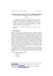
C1<br />
I1<br />
I2<br />
CSM<br />
(a) An example of <strong>in</strong>terior<br />
region elim<strong>in</strong>ation<br />
C2<br />
W<br />
4.1.3 Region-based elim<strong>in</strong>ation<br />
E E<br />
(b) PCTs from S after elim<strong>in</strong>ation<br />
Figure 4: Valid PCTs from S, E and <strong>in</strong>terior region<br />
S<br />
(c) Term<strong>in</strong>ation list from E<br />
Once the regions are identified, all PCTs and curves that are conta<strong>in</strong>ed <strong>in</strong> the regions are<br />
elim<strong>in</strong>ated (Lemma 4). In order to get the PCTs with<strong>in</strong> the regions, the values counterclockwise<br />
angle with respect to the SE l<strong>in</strong>e or parameter values of IOC are used. S<strong>in</strong>ce the<br />
PCTs are from the same start<strong>in</strong>g po<strong>in</strong>t, the angle and the parameter of IOC correlate. Firstly<br />
a range of parametric values is identified us<strong>in</strong>g the PCTs that contribute to the identification<br />
of regions. Then tangents fall<strong>in</strong>g with<strong>in</strong> or outside the range are elim<strong>in</strong>ated accord<strong>in</strong>gly. For<br />
curve elim<strong>in</strong>ation with<strong>in</strong> a region, typical <strong>in</strong>tersection check followed by ray shoot<strong>in</strong>g is done.<br />
Figure 4(b) and 4(c) show the rema<strong>in</strong><strong>in</strong>g PCTs from S and E after employ<strong>in</strong>g region-based<br />
elim<strong>in</strong>ation. Inner loops that are elim<strong>in</strong>ated us<strong>in</strong>g exterior regions R1 and R2 are shown as<br />
gray <strong>in</strong> Figure 3(b). Algorithm 1 describes the pseudocode for obta<strong>in</strong><strong>in</strong>g PCTs and process<strong>in</strong>g<br />
them.<br />
4.2 Process<strong>in</strong>g BTs<br />
BTs are computed from each PCT <strong>in</strong> the start<strong>in</strong>g list (which conta<strong>in</strong>s thus far processed<br />
PCTs, Figure 4(b)). A similar region elim<strong>in</strong>ation strategy is followed for BTs with some<br />
modifications to the region identification. Consider a <strong>path</strong> ζ, shown <strong>in</strong> Figure 5(a) from S<br />
to a po<strong>in</strong>t T on a curve CT G, which is an <strong>in</strong>complete potential SIP (i.e., the <strong>path</strong> has not<br />
yet reached the end po<strong>in</strong>t E). At and near T , CT G is concave. Let φ (clockwise or counterclockwise)<br />
be the direction <strong>in</strong>duced by ζ on CT G. Let NIF be the closest <strong>in</strong>flection po<strong>in</strong>t to<br />
T on CT G <strong>in</strong> the direction φ. Now T and NIF identify a concave portion of CT G.<br />
To identify the next set of potential <strong>path</strong>s for ζ, the set of bitangents from concave portion<br />
T NIF is computed. The bitangents that are not completely conta<strong>in</strong>ed <strong>in</strong> MCD and those that<br />
are not consistent with direction φ are removed. Let the start<strong>in</strong>g foot po<strong>in</strong>t of each bitangent<br />
be denoted by FST . The start<strong>in</strong>g curve, CST , for all bitangents is CT G. Let the end foot po<strong>in</strong>t<br />
and correspond<strong>in</strong>g end curve be denoted by FEN and CEN. Each bitangent is extended from<br />
8