Supplementary Web Material - Biometrics

Web-based supplementary materials for Calculating sample size
for studies with expected all-or-none nonadherence and selection
bias by Michelle D. Shardell and Samer S. El-Kamary
May 15, 2008
Web Appendix: Sample size calculations using exter-
nal or internal pilot data that accommodate noncom-
pliance
Sample size formulas and test statistics
FHF proposed methods for calculating sample size for normal and Poisson F while ac-
counting for variability of existing data. The approach of calculating “calibrated power”
for normal F with assumed equal variances by integrating out the variance estimator in
FHF Section 3 was motivated by external pilot data when ρc = 1. Many trials do not have
preliminary data, including compliance information, at the outset. Thus, one approach
for calculating sample size is to perform an unblinded internal pilot study as a source for
deriving assumptions about means, variances, and compliance. Interestingly, the critical
value for calibrated power in FHF for external pilot studies equals the exact “inflation
factor” in Zucker et al. (1999 p. 3502) needed for internal pilot studies (also calculated
by integrating out the variance estimator). To circumvent the numerical integration re-
quired for calibrated power/exact inflation factors, methods have been proposed utilizing
1

approximate inflation factors in sample size calculations when ρc = 1 under the assump-
tion of equal variances between groups (Wittes et al., 1999; Zucker et al., 1999; Miller,
2005). These authors also proposed adaptations of the t-test when internal pilot data are
collected to avoid elevated type I errors. However, no previous work has accommodated
noncompliance in this context.
In this Web Appendix, we adapt previously proposed approximate sample size formulas
for external and internal pilot data to accommodate noncompliance and unequal variances.
In the case of internal pilot studies, we also adapt two test statistics to accommodate
noncompliance. The first method adapted is the second-segment Stein (1945) (SS) method
described in Zucker et al. (1999). The second method adapted is the approach by Miller
(2005) in which bounded bias (BB) of the variance estimate is accommodated in the
sample size formula and t-test.
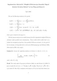
Assuming equal variances in both groups, ρc = 1, and r = 1, the original Stein (1945)
approach involved calculating
N = 2{(tα/2,2(np−1) + tβ,2(np−1))/δ} 2 S 2 p
+ 1, (1)
where S 2 p is the pooled variance estimate calculated from the pilot data, tq,ν is the 1−q
quantile of the t distribution with ν degrees of freedom, and np is the sample size per
group in the pilot study. Thus, the approximate inflation factor used in (1) to account for
variance uncertainty is {(tα/2,2(np−1) +tβ,2(np−1))/(zα/2 +zβ)} 2 , whereas the exact inflation
factor corresponding to calibrated power in FHF is {(zα/2 + zβ∗)/(zα/2 + zβ)} 2 , where
1 − β∗ is calibrated power (Zucker et al., 1999).
If the pilot study is internal, then ns = N − np additional observations per group are
collected, and the test statistic is then tStein = � N/2( ¯ Y1 − ¯ Y0)/Sp, to be compared with
tα/2,2(np−1). The SS procedure in Zucker et al. (1999) uses (1), but with a different test
2

statistic, and can only be used if some minimum sample size for the second segment (i.e.,
ns) is imposed. Let Dz = ( ¯ Yzs − ¯ Yzp) be the mean observed study outcome difference
in group z of the second segment data compared to the pilot data. Further, Let S 2 s
be the pooled variance estimate of the second-segment data. The test statistic is then
tSS = � N/2( ¯ Y1 − ¯ Y0)/SSS to be compared to tα/2,2ns, where
S 2 SS
�
−1
= (2ns) 2(ns − 1)S 2 npns
s +
N (D2 1 + D2 0 )
�
.
Before describing our adaptation of the SS approach, we describe the BB method by
Miller (2005). Assuming equal variances in both groups, ρc = 1, and r = 1, the approach
involved calculating v = 2{(Zα/2 +Zβ)/δ} 2 , and setting N = max{vS 2 p +1, np +ns(min)},
where ns(min) ≥ 0 is an arbitrary minimum for the second segment. Let S 2 be the pooled
variance estimate from all of the study data. Miller (2005) showed that − np−1
(np−2)v ≤
E(S 2 ) − σ 2 ≤ 0, where σ 2 is the true variance for both groups. The proposed correction
for this bias is the variance estimator S 2 BB = S2 + np−1
(np−2)v 1{N>np+n s(min)}, where 1{·} is the
indicator function, with test statistic tBB = � N/2( ¯ Y1 − ¯ Y0)/SBB, compared to tα/2,2(N−1).
We consider new sample-size formulas for internal and external pilot studies that
adapt (1) and Miller (2005) approaches. We also propose two adaptations of the t-
test that extend tSS and tBB for internal pilot studies. The extensions of the sample
size calculation involve 1) using the t inflation factor like in (1), 2) letting treatment-
group variances and sample sizes differ (and using the Welch approximation for degrees
of freedom), and 3) incorporating compliance-group proportion estimates. We calculate
a noncompliance corrected v, vnc = {(tα/2,νp + tβ,νp)/δˆρcp} 2 , where νp is the degrees of
freedom calculated with the Welch approximation using the pilot data, and ˆρcp is the
estimated proportion of compliers calculated from the pilot data.
For external pilot studies, the sample size formula for the control group is
3

N0 = vnc(S 2 0p + S2 1p /r) + 1. (2)
For internal pilot studies, we propose a formula that produces restricted designs, i.e.,
N0 > n0p (Wittes et al., 1999):
�
N0 = max vnc(S 2 0p + S2 1p /r) + 1, n0p
�
+ n0s(min) , (3)
where S 2 zp is the sample variance of group z calculated from the pilot data, nzp is the
sample size of the pilot data in group z, and n0s(min) is an arbitrary minimum sample
size for the control group second segment. We assume that the pre-specified ratio r is
maintained for both stages of the study so that n1p/n0p = n1s(min)/n0s(min) = r.
Our adaptation of tSS for internal pilot studies involves deriving group-specific variance
estimates. Let
S 2 zSS
�
−1
= (nzs) (nzs − 1)S 2 zs
nzpnzs
+ D
Nz
2 �
z .
The noncompliance SS (NSS) test statistic is then tNSS = (S 2 0SS /N0+S 2 1SS /N1) −1/2 ( ¯ Y1−
¯Y0), compared to tα/2,νNSS , where
νNSS =
(S2 0SS /N0 + S2 2
1SS /N1)
(S 2 0SS /N0) 2 /n0s + (S 2 1SS /N1) 2 /n1s
Note that nzs are the degrees of freedom for S 2 zSS and were hence used in νNSS instead
of nzs − 1.
Our adaptation of tBB involves accounting for the potential bias in two variance es-
timates for the special case of r = 1, thus n1p = n0p = np, n1s = n0s = ns, n1s(min) =
n0s(min) = ns(min), and N1 = N0 = N. We calculate the variance
4
.

S 2 0BB + S2 1BB = S2 0 + S2 1 + 2 np − 1
where the term −2 np−1
(νp−2)vnc
(νp − 2)vnc
1{N>np+n s(min)}, (4)
is an approximate bound for bias of S 2 0 + S 2 1 based on
the proof of theorem 1 in Miller (2005) using the Welch approximation of S 2 0p + S 2 1p to a
chi-square random variable. The derivation of (4) is found in the subsection below. The
noncompliance BB (NBB) test statistic is then tNBB = (S 2 0BB /N +S2 1BB /N)−1/2 ( ¯ Y1 − ¯ Y0),
compared to tα/2,νNBB , where
νNBB =
(S 2 0BB /N + S2 1BB /N)2
(S 2 0BB /N)2 /(N − 1) + (S 2 1BB /N)2 /(N − 1) .
The proposed sample size formulas involve adapting the approximate inflation factor
in (1) to handle unequal variances that may be due to noncompliance with selection bias.
However, use of the Welch approximation in sample size calculations and both tests in
the presence of noncompliance is not entirely accurate. When ρc = 1, the Welch degrees
of freedom are used to approximate the distribution of the variance of mean differences, a
sum of weighted chi-square random variables, to a chi-square random variable. However,
in the presence of noncompliance, the variance of mean differences is a sum of weighted
central and noncentral chi-square random variables, where the noncentrality parameters
depend on true adherence-subgroup means and compliance group distribution. The source
of this inaccuracy is a special case of averaging over a factor causing heterogeneity in the
treatment-specific outcome distribution. Even in cases with ρc = 1, other factors not
considered in the sample size calculation (e.g., sex, age, etc.) are averaged over that
may also cause heterogeneity in the outcome distribution. A closed-form approximate
method that is reasonably accurate in accounting for heterogeneity from noncompliance
is of practical utility, thus it is of interest to evaluate the performance of the proposed
procedures for different levels of noncompliance and selection bias.
5

Derivation of Bounded Bias Expression (4)
This subsection can be skipped without loss of continuity. From the work of Wittes
et al. (1999), the bias of S2 z for internal pilot studies with r = 1 can be expressed as
E(S2 z − σ2 �
(np−1)(S2 zp−σ
z) = E
2 � �
z)
= (np − 1)cov S np+ns−1
2 �
1
zp, , because ns is a random
np+ns−1
variable. Thus,
E{S 2 0 + S2 1 − (σ2 0 + σ2 1 )} = (np − 1)cov
�
S 2 0p + S2 1p ,
�
σ2 0 +σ
where we approximate E
2 1
S2 0p +S2 �
1p
⎡
⎢
= (np − 1)cov ⎢
⎣S2 0p + S2 1p ,
⎧
⎨
> (np − 1)cov
⎩ S2 0p + S 2 1p,
1
np + ns − 1
�
�
v(S2 0p +S
max
2 1p )
2ρ2 , np + ns(min) − 1
c
1
v(S 2 0p +S2 1p )
2ρ 2 c
= np − 1
v/(2ρ2 � � 2 σ0 + σ
1 − E
c)
2 1
S2 0p + S2 �
1p
�
≈ np − 1
v/(2ρ2 �
· 1 −
c ) νp
�
,
νp − 2
⎫
⎬
⎭
1
⎤
⎥
�⎥
⎦
by E � � νp
, where X is a chi-square random variable
X
with νp degrees of freedom. Therefore, E(X −1 ) = 1/(νp − 2). The inequality follows from
Lemma A.1 in Miller (2005). Estimating v/(2ρ 2 c) with vnc completes the derivation.
6

Simulation study
We assess the performance of our proposed sample size calculations and tests via extensive
simulation studies under a variety of specifications for ρc, selection bias, and variance
inequality. In all specifications, the sample size is calculated to detect δ = 0.5 with 80%
power, where µc1 = 0.5, µc0 = 0, and σ 2 c0 = σ2 n
= 1, using two-sided tests with α = 0.05.
Pilot studies were simulated with r = 1, n0p = n1p = 10, 20, 30, 50. For internal pilot
studies, the sample size was calculated using (3), where n0s(min) = 10. For external pilot
studies, (2) was used to calculate sample size. For each specification, 100,000 ‘studies’
were simulated to estimate empirical power and type I error of the naive t-test. For
internal pilot studies, tNSS and tNBB were also evaluated.
The empirical type I error for the approaches with internal pilot data is found in Web
Table 1. We see that both tNSS and tNBB are more conservative and control type I error
better than the naive t-test. However, like in Wittes et al. (1999) where ρc = 1, when nzp
and nzs are large, empirical type I error is approximately unbiased for the naive t-test. The
largest biases occurred when σ 2 c1 �= σ2 a . The tNSS and tNBB statistics perform similarly to
each other. The empirical power (when µc1 = 0.5 and µc0 = 0) for the approaches with
internal pilot data is found in Web Table 2. As in Wittes et al. (1999), when nzp is a
small percentage of the required sample size, the study is under-powered. In particular,
empirical power is lowest in the specification with ρc = 0.20, but improves with increasing
nzp. As in Zucker et al. (1999) where ρc = 1, tNSS performs well for attaining adequate
power when nzp is sufficient, at least 10% of the required sample size for the specifications
explored in this study, regardless of selection bias. Again, the performances of tNSS and
tNBB are similar.
The empirical type I error and power of the naive t-test for external pilot studies are
found in Web Table 3. We see that the approach performs well, and achieves close to
7

nominal power when nzp = 50 for all specifications studied except when ρc < 0.5 (i.e., the
specifications requiring the largest sample size). We also see that, like with internal pilot
studies, the median required sample size per group decreases with increasing nzp. This
result reflects that when nzp is larger compared to when it is smaller, inflation factors
are closer to one owing to larger degrees of freedom in (2) and more precise estimates of
variance and ρc from pilot data.
Conclusion
Although more accurate approximations for the distribution of a sum of weighted noncen-
tral chi-square variables have been proposed (e.g., Castaño-Martínez and López-Blázquez,
2005), their mathematical complexity limits their use and practicality for calculating sam-
ple size. Further, the simulation studies show that using the Welch approximation for
degrees of freedom in the inflation factor and resulting t-tests performs reasonably well
for controlling type I error and attaining desired power in the presence of noncompliance.
The main factor that impacts the performance of the methods is the ratio of nzp to the
total required sample size. If ρc is expected to be small, then nzp should be chosen to
have a sufficient number in each adherence subgroup to provide a reasonable estimate of
subgroup means and variances for precisely estimating treatment-group variances, partic-
ularly when large levels of selection bias are expected.
Zucker et al. (1999) discussed concerns about jeopardizing blinding for internal pi-
lot studies that are relevant here. In particular, unblinding may risk interim testing in
addition to sample size calculation, which further impacts type I error. The authors
noted that interim sample size calculation without testing can be allowed by disclosing
treatment-group variance estimates, but not interim mean differences. To adapt this rec-
ommendation to allow noncompliance, the interim compliance proportion estimate also
8

needs to be revealed.
References
Castaño-Martínez, A. and López-Blázquez, F. (2005). Distribution of a sum of weighted
noncentral chi-square variables. Test 14, 397-415.
Miller, F. (2005). Variance estimation in clinical studies with interim sample size reesti-
mation. Biometrics 61, 355-361.
Stein, C. (1945). A two-sample test for a linear hypothesis whose power is independent of
the variance. Annals of Mathematical Statistics 16, 243-258.
Wittes, J., Schabenberger, O., Zucker, D., Brittain, E., and Proschan, M. (1999). Internal
pilot studies I: Type I error rate of the naive t-test. Statistics in Medicine 18, 3481-
3491.
Zucker, D.M., Wittes, J.T., Schabenberger, O., and Brittain, E. (1999). Internal pilot
studies II: Comparison of various procedures. Statistics in Medicine 18, 3493-3509.
9

10
Table 1: Comparison of empirical type I error to nominal type I error (5%) with sample sizes calculated using Equation
3 with internal pilot data to detect δ = 0.5 with µc1 = 0.5 and µc0 = 0 where σ 2 c0 = σ2 n = 1, and ρn = ρa = (1 − ρc)/2.
Two groups compared using the naive t-test, tNSS, and tNBB. N = median sample size per group. Monte Carlo standard
error = 0.06% from 100,000 iterations.
nzp = 10 nzp = 20 nzp = 30 nzp = 50
ρc µa µn σ 2 c1 σ2 a N t tNSS tNBB N t tNSS tNBB N t tNSS tNBB N t tNSS tNBB
0.20 0.00 0.00 1.00 1.00 1671 5.06 5.05 5.05 1618 5.13 5.13 5.12 1586 4.95 4.93 4.94 1584 5.02 5.00 5.01
0.30 0.00 0.00 1.00 1.00 743 5.04 5.01 5.02 718 4.99 4.96 4.97 719 5.06 5.03 5.04 708 5.02 4.99 5.00
0.50 0.00 0.00 1.00 1.00 271 5.07 5.01 5.02 261 5.12 5.08 5.06 257 5.09 5.05 5.04 256 5.03 4.94 4.98
0.75 0.00 0.00 1.00 1.00 122 5.13 4.98 4.99 117 5.18 5.07 5.09 116 5.18 5.09 5.08 120 5.08 5.04 4.99
0.50 -0.25 0.00 1.00 1.00 274 5.00 4.97 4.97 264 5.06 4.98 5.00 260 5.10 5.06 5.06 258 5.05 5.00 5.00
0.50 -0.25 0.25 1.00 1.00 278 5.13 5.06 5.08 268 5.15 5.09 5.10 266 5.03 4.98 4.99 263 5.05 5.00 4.99
0.50 0.25 0.25 1.00 1.00 275 5.00 4.93 4.96 264 5.09 5.04 5.04 262 5.05 5.00 5.00 260 5.05 5.02 5.00
0.50 0.25 -0.25 1.00 1.00 280 4.99 4.96 4.94 268 5.05 5.02 5.01 266 5.10 5.04 5.04 263 4.98 4.94 4.94
0.50 0.50 -0.25 1.00 1.00 289 5.07 5.01 5.02 279 5.17 5.11 5.11 277 5.00 4.96 4.97 275 5.02 4.97 4.99
0.50 0.25 -0.50 1.00 1.00 290 5.02 4.97 4.97 279 5.03 4.98 4.97 277 4.92 4.88 4.88 274 4.85 4.83 4.82
0.50 0.50 -0.50 1.00 1.00 304 5.09 5.03 5.04 293 5.07 5.02 5.03 290 4.98 4.93 4.93 288 5.07 5.03 5.03
0.50 0.50 0.50 1.00 1.00 287 5.03 4.95 4.98 276 4.98 4.92 4.93 275 5.08 5.04 5.03 272 5.03 4.98 4.98
0.50 0.00 0.00 1.50 1.00 304 5.02 4.97 4.97 293 5.11 5.07 5.06 290 4.86 4.82 4.82 287 4.97 4.92 4.93
0.50 0.00 0.00 1.50 1.50 337 5.04 5.00 5.00 324 4.98 4.93 4.95 321 4.90 4.86 4.85 327 5.12 5.08 5.09
0.50 0.00 0.00 0.75 1.00 255 5.01 4.95 4.96 244 5.07 5.01 5.00 241 5.11 5.05 5.07 247 5.06 4.99 5.01
0.50 0.00 0.00 0.75 0.75 240 5.12 5.06 5.07 231 5.05 4.98 4.99 229 5.10 5.03 5.03 239 5.07 5.04 5.02
0.50 0.00 0.00 2.00 1.00 338 5.01 4.94 4.95 324 4.97 4.92 4.94 321 5.10 5.02 5.04 319 5.20 5.16 5.16
0.50 0.00 0.00 2.00 2.00 404 5.07 5.04 5.03 390 4.99 4.94 4.95 385 4.97 4.91 4.93 384 4.99 4.95 4.95
0.50 0.00 0.00 0.50 1.00 237 5.02 4.96 4.96 227 5.17 5.11 5.10 225 5.08 4.98 5.02 224 5.07 5.01 5.02
0.50 0.00 0.00 0.50 0.50 204 5.02 4.93 4.94 195 5.08 5.03 5.00 194 5.04 4.96 4.97 192 5.07 5.02 5.00
0.50 0.25 -0.25 0.75 0.75 245 5.01 4.94 4.95 235 5.12 5.06 5.06 234 5.00 4.97 4.94 240 5.02 4.99 4.97
0.50 0.25 -0.50 1.50 1.50 357 5.07 5.01 5.02 344 5.04 4.98 5.00 339 4.86 4.85 4.83 350 4.89 4.86 4.85
0.50 0.50 -0.50 2.00 2.00 438 4.92 4.87 4.88 420 4.93 4.89 4.89 418 5.01 4.99 4.98 423 4.92 4.89 4.89
0.50 0.50 -0.50 0.50 0.50 237 5.07 5.00 5.00 227 5.10 4.99 5.03 226 5.06 5.00 5.00 231 5.02 4.94 4.96
0.50 0.50 -0.50 2.00 0.50 339 5.13 5.08 5.09 326 5.08 5.03 5.04 322 5.02 4.99 4.98 327 5.23 5.21 5.20

11
Table 2: Comparison of empirical power to nominal power (80%) from studies with sample sizes calculated using Equation
3 with internal pilot data to detect δ = 0.5 with µc1 = 0.5 and µc0 = 0 where σ 2 c0 = σ2 n = 1, and ρn = ρa = (1 − ρc)/2.
Two groups compared using the naive t-test, tNSS, and tNBB. N = median sample size per group. Monte Carlo standard
error = 0.13% from 100,000 iterations.
nzp = 10 nzp = 20 nzp = 30 nzp = 50
ρc µa µn σ 2 c1 σ2 a N t tNSS tNBB N t tNSS tNBB N t tNSS tNBB N t tNSS tNBB
0.20 0.00 0.00 1.00 1.00 1685 69.35 69.35 69.32 1643 72.30 72.28 72.27 1628 73.98 73.96 73.95 1627 75.60 75.56 75.57
0.30 0.00 0.00 1.00 1.00 761 73.65 73.57 73.66 739 75.83 75.75 75.78 732 76.81 76.74 76.76 726 78.03 77.96 77.97
0.50 0.00 0.00 1.00 1.00 278 78.02 77.82 77.89 269 79.10 78.84 78.97 266 79.73 79.49 79.60 264 80.24 79.99 80.14
0.75 0.00 0.00 1.00 1.00 125 81.02 80.60 80.67 120 81.06 80.46 80.84 118 81.32 80.75 81.08 120 81.11 80.26 80.93
0.50 -0.25 0.00 1.00 1.00 285 77.77 77.58 77.64 275 78.52 78.33 78.42 273 79.39 79.16 79.28 271 79.72 79.46 79.62
0.50 -0.25 0.25 1.00 1.00 287 77.57 77.39 77.42 277 78.72 78.48 78.58 274 79.14 78.94 79.05 272 79.62 79.35 79.52
0.50 0.25 0.25 1.00 1.00 275 77.85 77.63 77.70 264 79.09 78.85 78.95 262 79.55 79.31 79.40 259 80.21 79.95 80.08
0.50 0.25 -0.25 1.00 1.00 287 78.65 78.47 78.53 276 79.73 79.50 79.61 274 80.32 80.10 80.21 271 80.98 80.72 80.88
0.50 0.50 -0.25 1.00 1.00 295 78.57 78.35 78.45 284 79.83 79.62 79.73 281 80.78 80.54 80.67 278 81.09 80.82 81.00
0.50 0.25 -0.50 1.00 1.00 306 78.64 78.44 78.51 291 79.89 79.66 79.79 288 80.83 80.53 80.71 286 81.35 81.13 81.25
0.50 0.50 -0.50 1.00 1.00 314 78.55 78.34 78.43 300 80.04 79.78 79.91 297 80.85 80.62 80.76 295 81.61 81.35 81.49
0.50 0.50 0.50 1.00 1.00 277 78.19 77.99 78.04 268 79.16 78.93 79.04 265 79.90 79.64 79.80 263 79.89 79.62 79.79
0.50 0.00 0.00 1.50 1.00 315 77.76 77.60 77.64 301 79.08 78.87 78.96 297 79.59 79.39 79.48 296 80.05 79.87 79.95
0.50 0.00 0.00 1.50 1.50 346 77.71 77.54 77.60 332 78.86 78.70 78.77 329 79.44 79.26 79.32 326 80.01 79.84 79.94
0.50 0.00 0.00 0.75 1.00 263 78.03 77.80 77.89 252 79.25 78.99 79.12 249 79.68 79.43 79.56 247 80.58 80.27 80.46
0.50 0.00 0.00 0.75 0.75 253 78.70 78.49 78.56 243 79.63 79.36 79.49 240 80.06 79.77 79.92 239 80.78 80.46 80.67
0.50 0.00 0.00 2.00 1.00 346 77.89 77.74 77.78 334 78.84 78.68 78.75 330 79.48 79.32 79.39 328 79.91 79.76 79.82
0.50 0.00 0.00 2.00 2.00 413 77.67 77.53 77.59 399 78.68 78.55 78.60 393 79.34 79.21 79.28 389 79.90 79.71 79.83
0.50 0.00 0.00 0.50 1.00 246 78.26 77.97 78.08 236 79.38 79.06 79.24 233 79.88 79.56 79.76 231 80.29 79.94 80.17
0.50 0.00 0.00 0.50 0.50 212 78.13 77.81 77.93 204 79.30 78.94 79.12 202 80.08 79.73 79.94 200 80.77 80.42 80.61
0.50 0.25 -0.25 0.75 0.75 252 78.32 78.08 78.19 243 79.93 79.65 79.80 241 80.50 80.21 80.38 240 81.35 81.08 81.22
0.50 0.25 -0.50 1.50 1.50 371 78.18 78.01 78.07 358 79.63 79.47 79.54 353 80.27 80.07 80.17 349 80.71 80.52 80.63
0.50 0.50 -0.50 2.00 2.00 447 78.42 78.27 78.32 430 79.53 79.39 79.46 425 80.18 80.03 80.12 422 80.74 80.55 80.66
0.50 0.50 -0.50 0.50 0.50 246 79.08 78.76 78.91 235 80.70 80.34 80.53 234 81.50 81.12 81.37 232 82.39 82.03 82.26
0.50 0.50 -0.50 2.00 0.50 347 78.89 78.71 78.77 333 79.96 79.77 79.86 330 80.39 80.20 80.29 326 81.42 81.21 81.34

12
Table 3: Comparison of empirical Type I error (αe), and power, (1−βe), to nominal Type I error (5%) and power (80%),
respectively, from studies with sample sizes calculated using Equation 2 with external pilot data to detect δ = 0.5 with
µc1 = 0.5 and µc0 = 0 where σ 2 c0 = σ2 n = 1, and ρn = ρa = (1 − ρc)/2. Two groups compared using the naive t-test.
NH0 = median sample size when the null hypothesis is true; NH1 = median sample size when the alternative hypothesis
is true. Monte Carlo standard error = 0.06% for αe and 0.13% for 1 − βe from 100,000 iterations.
nzp = 10 nzp = 20 nzp = 30 nzp = 50
ρc µa µn σ 2 c1 σ2 a NH0 αe NH1 1−βe NH0 αe NH1 1−βe NH0 αe NH1 1−βe NH0 αe NH1 1−βe
0.20 0.00 0.00 1.00 1.00 1676 5.10 1714 69.67 1651 4.94 1620 72.10 1633 5.04 1601 73.38 1582 5.01 1616 75.10
0.30 0.00 0.00 1.00 1.00 740 4.99 760 73.53 738 4.96 720 75.49 731 4.86 712 76.41 702 4.93 721 77.78
0.50 0.00 0.00 1.00 1.00 270 4.83 270 77.49 268 5.03 260 78.56 265 5.09 265 78.96 254 4.86 262 79.72
0.75 0.00 0.00 1.00 1.00 121 4.96 121 79.90 118 5.04 116 80.40 117 4.98 117 80.31 114 5.01 116 80.66
0.50 -0.25 0.00 1.00 1.00 275 4.91 275 77.81 274 5.12 262 78.59 272 5.06 272 79.04 257 4.97 269 79.75
0.50 -0.25 0.25 1.00 1.00 278 5.05 278 77.68 275 4.98 267 78.59 272 4.89 272 78.78 263 5.01 271 79.38
0.50 0.25 0.25 1.00 1.00 274 5.01 274 77.64 264 4.95 263 78.74 260 5.08 260 79.02 259 4.88 258 79.55
0.50 0.25 -0.25 1.00 1.00 279 5.10 279 77.42 276 4.98 268 78.43 271 4.91 271 79.06 263 5.20 271 79.49
0.50 0.50 -0.25 1.00 1.00 289 5.00 289 77.45 282 4.99 278 78.54 279 4.92 279 78.93 274 4.96 278 79.52
0.50 0.25 -0.50 1.00 1.00 289 4.91 289 77.38 290 5.00 278 78.35 288 4.93 288 78.80 273 4.93 285 79.57
0.50 0.50 -0.50 1.00 1.00 304 4.95 304 77.27 301 4.98 293 78.43 296 5.10 296 78.91 287 5.04 295 79.38
0.50 0.50 0.50 1.00 1.00 286 4.97 286 77.45 267 4.93 275 78.54 264 5.07 264 78.97 270 4.99 262 79.50
0.50 0.00 0.00 1.50 1.00 303 4.99 311 77.70 299 5.11 291 78.74 297 4.97 288 79.10 287 5.06 294 79.49
0.50 0.00 0.00 1.50 1.50 336 4.93 345 77.49 323 4.93 323 78.49 328 5.03 320 78.98 325 5.01 326 79.41
0.50 0.00 0.00 0.75 1.00 252 5.03 260 77.42 243 4.89 243 78.33 248 4.95 240 79.16 246 4.86 247 79.50
0.50 0.00 0.00 0.75 0.75 240 4.85 240 77.79 230 4.92 230 78.48 238 4.92 226 78.82 238 5.00 238 79.47
0.50 0.00 0.00 2.00 1.00 338 4.90 347 77.85 332 5.06 324 78.67 329 4.99 321 78.93 318 5.03 326 79.55
0.50 0.00 0.00 2.00 2.00 402 5.02 410 77.31 397 4.94 389 78.60 394 5.00 386 79.18 381 4.96 390 79.48
0.50 0.00 0.00 0.50 1.00 236 5.04 244 77.04 235 4.99 227 78.16 232 5.09 224 78.83 223 4.93 231 79.40
0.50 0.00 0.00 0.50 0.50 202 5.01 211 77.52 203 4.99 194 78.44 201 5.01 193 79.01 191 5.03 199 79.91
0.50 0.25 -0.25 0.75 0.75 244 4.90 252 77.20 234 5.00 234 78.68 240 5.02 232 79.06 239 5.16 239 79.40
0.50 0.25 -0.50 1.50 1.50 357 5.16 370 77.17 344 4.97 344 78.29 351 4.91 339 78.96 350 5.05 349 79.30
0.50 0.50 -0.50 2.00 2.00 438 4.93 447 77.17 418 4.93 418 78.29 425 4.96 416 79.17 421 4.99 422 79.53
0.50 0.50 -0.50 0.50 0.50 237 4.87 245 76.75 226 4.95 226 78.17 233 5.12 225 78.77 231 5.06 231 79.44
0.50 0.50 -0.50 2.00 0.50 340 4.99 348 77.40 324 5.07 324 78.53 329 5.02 321 79.09 327 5.06 327 79.52