Marine Pollution Bulletin - ARC Centre of Excellence for Coral Reef ...

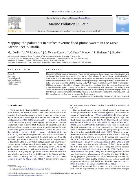
Mapping the pollutants in surface riverine flood plume waters in the Great 

Barrier Reef, Australia 

M.J. Devlin a,⇑ , L.W. McKinna b , J.G. Álvarez-Romero a,d , C. Petus a , B. Abott c , P. Harkness a , J. Brodie a 

a 

Catchment to Reef Research Group, TropWater, ACTFR, James Cook University, Townsville, QLD, Australia 

b 

Remote Sensing and Satellite Research Group, Department of Applied Physics, Curtin University, Perth, WA, Australia 

c 

Landscape & Community Ecology, CSIRO Ecosystem Sciences, Townsville, Australia 

d 

Australian Research Council Centre of Excellence for Coral Reef Studies, James Cook University, Townsville, QLD, Australia 

article info 

Keywords: 

River plume 

Terrestrial runoff 

Land-based threat 

Pollutant exposure 

MODIS images 

1. Introduction 

abstract 

The Great Barrier Reef (GBR) like many other coral reef ecosystems 

around the world is under stress from three main threats, 

associated with anthropogenic activities: over-harvesting of marine 

resources, climate change and contaminants in terrestrial runoff 

(Brodie et al., 2008, 2011; Fabricius, 2011; Pandolfi et al., 2003). 

The dominance of grazing and cropping agriculture on the GBR 

catchment raises concerns that discharge of nutrients and other 

pollutants from the adjacent catchment areas has increased drastically 

due to agricultural development over the last 150 years (Brodie 

et al., 2011; Kroon et al., 2011; Haynes et al., 2000; McKergow 

et al., 2005). The delivery of pollutants from the GBR catchments is 

regionally specific, with increased dissolved nutrients from the 

fertilised agriculture dominant in the Wet Tropics region (north 

of Townsville), the Mackay Whitsundays region and lower Burdekin 

catchment, and sediment loss from the larger Dry Tropics region 

(mainly via the Burdekin and Fitzroy rivers), where the 

predominant land use is cattle grazing (Kroon et al., 2011; Waterhouse 

et al., 2012) (Fig. 1). Significant concentrations of pesticides 

have also been measured in the GBR between the Fitzroy and Barron 

rivers (Kennedy et al., 2012; Lewis et al., 2009; 

Lewis et al., 2012a; Shaw et al., 2010). A comprehensive review 

⇑ Corresponding author. 

E-mail address: michelle.devlin@jcu.edu.au (M.J. Devlin). 

Marine Pollution Bulletin 65 (2012) 224–235 

Contents lists available at SciVerse ScienceDirect 

Marine Pollution Bulletin 

journal homepage: www.elsevier.com/locate/marpolbul 

0025-326X/$ - see front matter Crown Copyright Ó 2012 Published by Elsevier Ltd. All rights reserved. 

http://dx.doi.org/10.1016/j.marpolbul.2012.03.001 

The extent of flood plume water over a 10 year period was mapped using quasi-true colour imagery and 

used to calculate long-term frequency of occurrence of the plumes. The proportional contribution of riverine 

loads of dissolved inorganic nitrogen, total suspended sediments and Photosystem-II herbicides 

from each catchment was used to scale the surface exposure maps for each pollutant. A classification procedure 

was also applied to satellite imagery (only Wet Tropics region) during 11 flood events (2000– 

2010) through processing of level-2 ocean colour products to discriminate the changing characteristics 

across three water types: ‘‘primary plume water’’, characterised by high TSS values; ‘‘secondary plume 

water’’, characterised by high phytoplankton production as measured by elevated chlorophyll-a (chl-a), 

and ‘‘tertiary plume water’’, characterised by elevated coloured dissolved and detrital matter (CDOM + D). 

This classification is a first step to characterise flood plumes. 

Crown Copyright Ó 2012 Published by Elsevier Ltd. All rights reserved. 

of the current status of water quality is provided in Brodie et al. 

(2012a). 

Riverine flood plumes (hereafter flood plumes) are important 

pathways for terrestrial materials entering the sea, and a dominant 

source of coastal pollutants (Warrick et al., 2004). Discharge of pollutants 

to the GBR occurs overwhelmingly during the large river 

flood flows associated with the North Queensland wet season 

(Devlin and Schaffelke, 2009; Mitchell et al., 2005; Packett et al., 

2009). More than 90% of the nutrients sourced from the land enter 

the GBR lagoon during this time; consequently, river concentrations 

of different forms of nitrogen and phosphorus peak during 

these high-flow periods (Mitchell et al., 2005). Affected areas depend 

on the extent of the surface plume water, which is primarily 

dependent on the catchment size, the frequency and intensity of 

the peak flow events, and the prevailing wind and current conditions 

(Brodie et al., 2010; Devlin and Brodie, 2005; Wolanski and 

Jones, 1981). Investigating the influence of flood plumes within 

the GBR has been carried out sporadically for several decades 

(Brodie and Mitchell, 1992; Devlin et al., 2001; Devlin et al., 

2012; Wolanski and Jones, 1981), and monitoring of flood plumes 

now forms an integral component of a multidisciplinary GBR monitoring 

program (Johnson et al., 2011). Monitoring activities include 

ambient water quality measurements, inshore coral and 

seagrass monitoring and herbicide detection (Johnson et al., 

2011; Kennedy et al., 2012; Schaffelke et al., 2012). 

Ecological impacts of flood plumes on coral reefs and seagrass 

beds can be experienced as either acute, short-term changes

associated with formation of high-nutrient, high-sediment, lowsalinity 

flood plumes or the more chronic impacts associated with 

changes in long-term water quality concentrations. Acute stress 

from flood plumes on marine ecosystems include prolonged freshwater 

exposure, decreased light availability and smothering by 

high sedimentation during flood events or due to resuspension of 

terrigeneous fine sediments by wind, waves and tides in the period 

after the flood (Cooper et al., 2007, 2009; Fabricius, 2005). Largescale 

mortality events associated with low salinity through flood 

conditions have been documented for coral reefs (Berkelmans, 

2009; Byron and O’Neill 1992; van Woesik et al., 1995). Flood 

events with excess sediment and nutrient loads have also been 

associated with local declines of GBR seagrasses (McKenzie et al., 

2010; Schaffelke et al., 2005; Waycott et al., 2005) and recently 

linked with increased mortality of dugongs and sea turtles in the 

GBR (Bell and Ariel, 2011; McKenzie et al., 2010, 2011). 

Chronic exposure of corals to increased levels of nutrients, sedimentation 

and turbidity may affect certain species that are sensitive 

or vulnerable to changes in environmental conditions. This 

may lead to medium and long-term impacts such as reduced densities 

of juvenile corals, subsequent changes in community composition, 

decreased species richness and shifts to communities that 

are dominated by more resilient coral species and macroalgae 

(De’ath and Fabricius, 2010; DeVantier et al., 2006; Fabricius, 

2005; van Woesik et al., 1999). Recent work has linked an increase 

in long-term turbidity to the export and availability of finer sediment 

out of the large Dry Tropic regions (Fabricius, 2011; Fabricius 

et al., in review; Lambrechts et al., 2010; Wolanski et al., 

2008).Other long-term ecological impacts can be seen in the proliferation 

of Crown of Thorns Starfish (COTS) in areas which are regularly 

exposed to excess anthropogenic nutrient loads (Brodie 

et al., 2005; Fabricius et al., 2010). 

Flood plume waters generally move into the GBR as buoyant 

freshwater masses and are usually constrained in the top surface 

layer until dissipated or eventually mixed into the water column 

(Devlin and Brodie, 2005). For this reason, water sampling typically 

focuses on the top surface layer of the flood plumes, and remotely 

sensed data (e.g., satellite imagery) retrieved from surface waters 

can be used to characterise flood plumes. Ocean colour satellite 

imagery provides large-scale information on the movement and 

composition of flood plumes. It provides frequent regional overviews 

that enable effective and long-term analysis of flood plume 

spatial and temporal distribution based on water quality parameters 

that can be measured from space (Lihan et al., 2008). River 

flood plumes have been mapped successfully from remotely 

sensed data in a number of different coastal environments around 

the world (Andrefouet et al., 2002; Chérubin et al., 2008; Paris and 

Chérubin, 2008; Petus et al., 2010; Soto et al., 2009; Thomas and 

Weatherbee, 2006) to study the spatial extent, movement and fate 

of riverine flow into coastal waters. The use of remote sensing 

methods is thus relatively cost-effective and informative for a variety 

of detection, monitoring and information gathering exercises. 

In the GBR, both quasi-true colour (hereafter true colour) satellite 

images and derived water quality level-2 (L2) products have been 

utilised to map and characterise the distribution of GBR flood 

plumes (Devlin et al., 2012; Qin et al., 2007). 

In combination with in situ sampling of flood plumes, remotely 

sensed data has provided an additional source of data related to 

the movement and composition of flood plumes in GBR waters 

(Bainbridge et al., 2012; Brodie et al., 2010; Devlin et al., 2012; Schroeder 

et al., 2012), particularly because spatial coverage from vessel 

sampling is usually limited due to cost and adverse weather 

conditions. Flood plumes have been mapped and the coverage of 

GBR ecosystems visually assessed using satellite imagery (Devlin 

and Schaffelke, 2009). A combination of aerial surveys and satellite 

imagery has also been employed in the GBR to determine areas of 

M.J. Devlin et al. / Marine Pollution Bulletin 65 (2012) 224–235 225 

marine coastal ecosystems exposed to flood plumes (Brodie et al., 

2010; Devlin et al., 2001; Devlin and Brodie, 2005; Schroeder 

et al., 2012). 

Complementary water samples collected from within the flood 

plume have been analysed for contaminants of concern (Devlin 

et al., 2001; Devlin and Schaffelke, 2009) and have provided information 

on the length of time that inshore GBR ecosystems can be 

exposed to high concentrations of pollutants carried in flood 

plumes. Using in situ water quality measurements, the variable 

water characteristics of flood plumes in the GBR have been categorised 

as a gradient of water types (Devlin and Schaffelke, 2009; 

Devlin et al., 2012). Three main water types have been described: 

primary waters which are typically near-shore, turbid, low salinity 

waters; secondary waters which are less turbid and typically contain 

elevated chl-a biomass due to increased primary production; 

and tertiary waters, considered to be riverine influenced waters 

characterised by lower values of chl-a and CDOM in comparison 

with primary and secondary types, but still above ambient dry season 

values (Devlin and Schaffelke, 2009; Devlin et al., 2012). 

The main objective of this study is to map the spatial and temporal 

influence of surface flood plume water quality in the GBR. 

Pollutant load and areal extent of flood plumes delineated from satellite 

imagery are combined to estimate the level of exposure of 

surface waters to TSS, DIN and Photosystem-II (PSII) herbicides. 

The number of coral reefs and seagrass beds found in the areas 

with different categories of surface exposure is quantified for each 

pollutant for the whole GBR. Satellite products are further processed 

to map proxies of phytoplankton production, coloured dissolved 

and detrital matters and total suspended sediment 

concentration in GBR coastal and inshore waters, which in turn 

are used to discriminate the changing water quality characteristics 

across the defined ‘‘primary’’, ‘‘secondary’’ and ‘‘tertiary’’ water 

masses (hereafter water types) commonly found through GBR 

flood plumes (Devlin et al., 2012). 

2. Methods 

2.1. Study area 

A number of rivers drain into the GBR, all of which vary considerably 

in length, area of catchment, and flow intensity and frequency. 

The frequency and duration of high river flow periods 

influence the extent and evolution of the flood plumes that impinge 

on the GBR through the wet season (defined hereafter as 

the period between November and April inclusive). The GBR catchment 

has been divided into six large areas defined as Natural Resource 

Management (NRM) regions (Fig. 1), each with a set of 

land use/cover, biophysical and socio-economic characteristics 

which define that area. The Cape York region is largely undeveloped 

and is considered to have the least impact on GBR ecosystems 

from existing land based activities. In contrast, the Wet Tropics, 

Burdekin, Mackay Whitsunday, Fitzroy and the Burnett-Mary regions 

are characterised by extensive agricultural land uses including 

cattle grazing, sugar cane, bananas, other horticultural 

cropping, grains and cotton, mining, and urban development (Brodie 

et al., 2009a). Each of these activities contributes varying 

amounts of land-based pollutants to the GBR through the wet season. 

Wet Tropic catchments, located between Townsville and 

Cooktown, have frequent storm and runoff events in generally 

short, steep catchments, and thus more direct and frequent linkages 

to coastal environments. In the Dry Tropic catchments, the 

major flow events may occur at intervals of years, with long lag 

times for the transport of material through these large catchments 

(Brodie et al., 2009a). High river flows occur at a frequency of 0.25 

per year for Dry Tropics rivers including the Fitzroy and Burdekin

226 M.J. Devlin et al. / Marine Pollution Bulletin 65 (2012) 224–235 

Fig. 1. The extent of the Great Barrier Reef catchment and marine area with the Regional Natural Resource Management (NRM) regions identified for the whole of GBR 

including Cape York, Wet Tropics, Burdekin, MackayWhitsunday, Fitzroy and Burnett-Mary regions. Note the variable flow characteristics of three main rivers of the GBR, 

including Tully River (Wet Tropics), Burdekin River (Dry Tropics) and the Fitzroy River (Dry Tropics). Events are identified as days where the daily flow equal or exceeded the 

95th percentile value of flow (calculated from the period 1991–2010). 

to 3 flows per year for Wet Tropics’ rivers such as the Tully (Fig. 1). 

The number of days in an event, as described by the number of 

days above the long-term 95th percentile measurement is influenced 

by both the size of the catchment and the intensity and 

duration of the event. 

Ambient water quality conditions within the GBR are typically 

associated with low concentrations of dissolved inorganic nutrients, 

chl-a and TSS. Inshore (ambient) water quality concentrations 

(Furnas et al., 2011; Schaffelke et al., 2011, 2012) are significantly 

lower than those typically measured in flood plumes (Devlin and 

Brodie, 2005). Recent work by Furnas et al. (2011) reported ambient 

median concentrations of DIN (0.04–0.07 lM), TSS (1.2– 

1.7 mg L 1 ) and chl-a (0.36–0.44 lgL 1 ) for the inshore Cape York 

and Wet Tropics regions. These values are depth-integrated and 

whilst not directly comparable, show that conditions outside of 

the high-flow periods can be nutrient-depleted with available 

nutrients being rapidly assimilated by phytoplankton. Water quality 

concentrations, including TSS, coloured dissolved organic matter 

(CDOM), dissolved nutrients and chl-a typically decrease from 

inshore to offshore (Brodie et al., 2007; De’ath and Fabricius 

2008; Furnas, 2003), and also tend to be much lower in the northern, 

less developed Cape York region. In contrast, water quality 

parameters measured within flood periods are typically 1–100 

times higher than ambient concentrations, with water quality concentrations 

in flood plumes linked to catchment source, prevailing 

weather and the movement of the surface plume water (Devlin

et al., 2001; Devlin and Brodie, 2005; Devlin and Schaffelke, 2009; 

Schaffelke et al., 2012). 

2.2. High-flow conditions 

The frequency and spatial extent of flood plumes is mainly driven 

by the size of flow and the frequency at which the rivers 

achieve high-flow conditions. For this study, periods of high-flow 

were defined as those dates where the daily flow in megalitres 

(ML) exceeded the 95th percentile calculated over a period of 

20 years (1990–2010). Flow data was made available from the 

Queensland State Government river flow program (http:// 

www.watermonitoring.derm.qld.gov.au/host.htm). High-flow periods 

in the GBR can last from days to weeks depending on the size 

of the event and the catchment characteristics (Devlin et al., in 

press) and thus for this study we only considered flood plumes 

occurring within these periods. 

2.3. Satellite imagery 

The main catalogue of ocean colour satellite imagery used was 

that of the Moderate Resolution Imaging Spectroradiometer 

(MODIS) on-board the NASA Earth Observation System Terra and 

Aqua spacecrafts. Level-0 (L0) data corresponding to images during 

high-flow periods recorded between 2001 and 2010 were acquired 

from NASA’s Ocean Colour Browse website (http://www.oceancolor.gsfc.nasa.gov/cgi/browse.pl?sen=am). 

The number of data available 

during high flood periods was also constrained to dates 

associated with low cloud cover over our study area, with a maximum 

of 11 MODIS scenes finally selected and processed as follows. 

True colour images and L2 products (chlorophyll concentration 

(chl-a), coloured dissolved and detrital matter absorption coefficient 

(aCDOM-D) and two TSS proxies) were derived from L0 data 

using SeaWiFS Data Analysis System v5.4 – SeaDAS (Baith et al., 

2001). A combined near-infrared to short-wave infrared (NIR– 

SWIR) correction scheme (Wang and Shi, 2007) was applied to level-1 

products to overcome the atmospheric correction issues above 

turbid waters, commonly found in the nearshore regions of the GBR. 

2.4. Estimating surface exposure of flood plume waters in the GBR 

The distribution of flood plumes and areas most likely to be exposed 

to particular pollutants were calculated by the mapping of 

surface flood plume water based on true colour satellite images 

in combination with catchment pollutant load information. The 

process entails three steps (Fig. 2): 

2.4.1. Calculating the proportional contribution of pollutant loads from 

GBR catchments 

Load data from five NRM regions discharging directly into the 

GBR (Burnett-Mary was not included in this analysis) was summarised 

for the three main pollutants (TSS, DIN and PSII herbicides) 

using modelled and monitored load data as reported in Brodie 

et al. (2009b), Kroon et al. (2011), and Waterhouse et al. (2012). 

The annual means of the long-term load data for each pollutant 

was calculated for each NRM region. Following this, the proportional 

pollutant load (PL) contribution of each region, with respect 

to the overall GBR pollutant load, was estimated. For example, the 

Wet Tropics region contributes 0.16, 0.30 and 0.39 of the annual 

anthropogenic load of TSS, DIN and PSII herbicides respectively 

when scaled against the GBR-wide pollutant load (Fig. 2, step 1). 

2.4.2. Mapping the distribution and frequency of surface flood plume 

waters 

Visual interpretation of true colour satellite images was performed 

to identify and delineate the full areal extent of the surface 


GBR flood plumes (Brando et al., 2010; Devlin and Schaffelke, 

2009; Devlin et al., 2012). Mapped flood plumes (i.e., only those 

associated with high-flow events) were overlaid to calculate the 

long-term frequency of occurrence (P x, corresponding to the number 

of times any given area/pixel of the GBR was covered by flood 

plumes) over a period of 10 years (2001–2010). The frequency of 

occurrence of flood plumes was aggregated into frequency classes 

(F n), where the class value was calculated from number of 

plumes normalised to four equal-interval frequency classes (see 

Fig. 2, step 2). 

2.4.3. Estimating the surface exposure for each pollutant 

Surface exposure for each pollutant was estimated by scaling 

the pollutant load (PL) contribution against the frequency class of 

the flood plume distribution (Fn) within each NRM region (Fig. 2, 

step 3). A quantitative surface exposure (E) value for TSS, DIN 

and PSII herbicides was calculated for each pixel. Based upon these 

surface exposure values, each pixel was assigned one of four exposure 

types, ‘‘very high’’, ‘‘high’’, ‘‘moderate’’ and ‘‘low’’ for TSS, DIN 

and PSII herbicides, respectively. Note that DIN surface exposure 

values are not presented for Cape York due to the high error associated 

with the modelled anthropogenic load from this region 

(Waterhouse et al., 2012) and that the PSII herbicide load from 

Cape York was assumed to be zero and thus not assigned to any 

exposure category. 

2.5. Quantifying exposure of selected marine ecosystems to pollutants 

in flood plumes 

The surface distribution of the surface exposure (one for each 

pollutant: TSS, DIN, and PSII) were overlaid with maps of current 

distribution of coral reefs and seagrass beds to calculate the number 

and area of reefs and seagrass exposed to each surface exposure 

category (see Fig. 2). Coral (GBRMPA 2009) and seagrass 

(NFC 2009) distribution maps were provided as shapefiles by the 

Great Barrier Reef Marine Park Authority. Coral reefs and seagrass 

beds located outside of any of the mapped flood plumes were 

deemed ‘‘un-exposed’’ and quantified accordingly. 

2.6. Characterising water types within GBR flood plumes 

Semi-analytical algorithms to produce L2 products were applied 

to the 11 atmospherically corrected MODIS images (only those 

captured over the Wet Tropics marine areas during periods of 

high-flow and negligible cloud coverage) to map the inshore 

waters constituents and delineate the different GBR flood plume 

water types (i.e., primary, secondary and tertiary) as defined in 

Devlin and Schaffelke (2009) and Devlin et al. (2012). 

Four L2 products were mapped to characterise the three GBR 

typical surface waters types using SEADAS. The normalized 

water-leaving radiance at 667 nm (nLw_667, lWcm 2 nm 1 sr 1 ) 

was first mapped. This parameter is assumed to be effective to 

trace suspended particulate matter (Li et al., 2003) and has been 

positively correlated with TSS values and used to characterise flood 

plume water types (Devlin et al., 2012). The particulate backscattering 

coefficient at 555 nm (bbp_555, m 1 ), less sensitive to dissolved 

material, was obtained using the QAA model (Lee et al., 

2002)and used as a second proxy for particulate load (D’Sa et al., 

2007; Shanmugam et al., 2011). Chlorophyll-a concentration 

(lgL 1 )was obtained using the GSM01 model (Maritorena et al., 

2002) and used as a proxy of primary production. Finally, the 

absorption coefficient of coloured dissolved and detrital matter 

(aCDOM + D, m 1 ) at a wavelength of 443 nm was calculated based 

on the quasi-analytical algorithm (QAA) described in Lee et al. 

(2002). This parameter, related to the concentration of coloured 

dissolved and detrital matter in water, has been shown to be a


Fig. 2. Process of mapping the exposure of surface pollutants in flood plume waters. Annual load data is calculated as a proportional contribution based on catchment load in 

respect to overall GBR load. The load information is integrated with the surface distribution of flood plumes in the GBR. Surface mapping is taken over the period 2001–2010. 

good proxy for salinity (Schroeder et al., 2012), and thus useful to 

delineate the maximum freshwater effected extent of flood 

plumes. Performance of algorithms selected to map the chl-a concentrations 

and the CDOM + D absorption coefficient are limited 

due to the high complexity of the inshore waters but they are 

the best readily available algorithms which allow satellite analysis 

of the flood plume waters constituents in the GBR (Qin et al., 2007). 

Furthermore, precision of these algorithms are assumed to increase 

as the flood plume moved from turbid water (i.e., high TSS coastal 

waters) to offshore clearer waters. 

Combination of the L2 products (chl-a, aCDOM + D, nLw_667, 

bbp_551) obtained during the 11 flood events were used to characterise 

the three GBR typical surface waters types (Devlin and 

Schaffelke, 2009; Devlin et al., 2012). For each water type, thresholds 

values of nLw_667, bbp_551, CDOM + D and chl-a that best 

discriminated the gradients of TSS, chl-a, CDOM commonly found 

through flood plumes were determined empirically and adjusted 

until clear separation of the three water types was achieved. The 

extent and frequency of the different waters types in the GBR inshore 

waters were finally computed as described in Fig. 2 (step 

2) and maps depicting frequency of occurrence of primary and secondary 

water types were produced. Due to the relatively limited 

presence of the tertiary water type (i.e., occurring mostly in the 

edge or outer flood plume), the frequency map for tertiary water 

was not calculated. However, a map showing the frequency of 

the full flood plume (i.e., combined maps of the 3 water types) 

was produced (Fig. 5). 

2.7. Variation in in situ water quality characteristics between water 

types 

Water quality data collected in situ over the 9-year period as 

part of the GBR Marine Monitoring Program within the Wet Tropics 

NRM and over the main flood events of the wet season were 

identified. Chl-a, TSS and CDOM field data were assigned to a water 

type based on the location of the in situ site against the satellite 

water type map. The mean in situ water quality values (±2SE) 

within each water type were plotted to validate the delineation 

of water types obtained from the satellite images, and confirm 

the potential of MODIS L2 products to monitor gradients of water 

quality data measured in situ through GBR flood plumes. 

3. Results 

3.1. Estimating surface exposure of flood plume waters 

Flood plumes in the GBR lagoon can extend from the Cape York 

to the Burnett Mary regions, with these waters occasionally moving 

beyond the mid-shelf reef system (Fig. 3). Inshore areas within 

20 km are, unsurprisingly, areas which are most likely to see frequent 

flood plume water inundation, though previous work has 

shown that the timing of the plume inundation and the water quality 

composition of the plume differ significantly between river 

source, inshore, and offshore areas.

Measured and/or modelled pollutant loads for each catchment 

and region have been calculated (Brodie et al., 2009a) for the three 

pollutants of concern (DIN, TSS and PSII herbicides) (see Fig. 4). 

These load estimates identified the two large dry catchments 

(Burdekin and Fitzroy) as the primary source of TSS to the reef, 

with proportional contributions of 42% and 29%, respectively. DIN 

loading is elevated in catchments that are dominated by fertilised 

agriculture, particularly in the Wet Tropics and the lower Burdekin 

catchments. This is manifested in the high proportional contribution 

of both NRMs to DIN (i.e., 30% for the Wet Tropics and 39% 

for the Burdekin). PSII herbicides are exported from all agricultural 

catchments, with the pesticide load related to the agricultural 

activity (Lewis et al., 2009), indicating that the Mackay Whitsunday 

and Wet Tropics NRMs are the major contributors ( 38% each), 

followed by the Burdekin (19%). These values are reflected in the 

calculated surface exposure to each pollutant within each marine 

NRM (Fig. 4). 

Surface exposure mapping identifies up to 5970 km 2 and 

5131 km 2 of the marine areas of the Wet Tropics and Burdekin regions, 

respectively, which are exposed to flood plumes carrying 

high DIN loads (i.e., areas classified as ‘‘high’’ or ‘‘very high’’ exposure 

to DIN). These areas represent 19% and 11% of the total marine 

portion of the Wet Tropics and Burdekin regions, respectively. The 

surface mapping also indicated that up to 5,690 km 2 (12%) of the 

marine area of the Mackay Whitsunday region and up to 

2538 km 2 (8%) of the Wet Tropics are classified as ‘‘very high’’ 


Fig. 3. The frequency of flood plumes in the GBR. Darker colours denote a higher occurrence of plumes in that area. High exposure areas are located inshore between Cape 

York and Fitzroy catchments (10–25 km inshore). 

exposure for PSII herbicides. Furthermore up to 5,131 km 2 (11%) 

of the Burdekin and 7998 km 2 (9%) of the Fitzroy regions are classified 

as ‘‘high’’ to ‘‘very high’’ exposure for TSS (Table 1). 

The total area and number of reefs and seagrass beds that are 

located within each exposure category depends on the proximity 

of each ecological system to the area of riverine influence. Within 

our mapping analysis we were able to determine the exposure of 

coral reefs and seagrass beds to flood plumes within each NRM region. 

The Wet Tropics region was found to have a large number of 

features (174 coral reefs and 98 seagrass beds) within the high to 

very high exposure category for DIN due to the close proximity 

of the reefs, the high frequency of occurrence of flood plumes that 

are experienced in the Wet Tropics and the high proportional load 

of DIN. The Burdekin region was found to have the highest number 

of reefs (127) and seagrass beds (135) located in the ‘‘moderate’’ to 

‘‘very high’’ exposure category to TSS. The highest number of reefs 

(415) and seagrass beds (173) within the ‘‘high’’ to ‘‘very high’’ categories 

for PSII herbicide exposure were found in the Mackay 

Whitsunday region (Table 1). Numbers of reefs within the ‘‘low’’ 

exposure category or that had not been exposed to flood plumes 

through this study are high, particularly for coral reefs as the 

majority of the coral reefs are outside of the ‘‘high’’ to ‘‘very high’’ 

exposure categories for all pollutants. In contrast, about half of the 

seagrass beds are found in those ‘‘high’’ to ‘‘very high’’ categories, 

illustrating the vulnerability of inshore seagrass beds to pollutants 

carried in flood plumes (Table 1).


Fig. 4. The distribution of the four categories of surface exposure for each of the pollutants (TSS, chl-a and PSII herbicides). Exposure is scaled from high to low with the 

highest exposure related to the highest flood plume extents (>10) and the highest pollutant loads. Note that there is no exposure to PSII herbicides in Cape York water due to 

the very low area of fertilised agriculture. DIN loads in Cape York have very high levels of uncertainty (Waterhouse et al., 2012) and are not reported here. 

3.2. Characterising water types within Wet Tropics flood plumes 

Within the Wet Tropics, the mapping of the extent and frequency 

of the different waters types into the GBR inshore waters 

revealed the primary water type occurs parallel to the coast predominately 

in a small band of no more than 25 km (Fig. 5b). The 

secondary water type also occurs parallel to the coast however, 

reached a greater distance offshore of up to 100 km (Fig. 5c). The 

greatest extent of secondary water was found to occur north of 

the Barron River and north of the Tully-Murray and Johnstone Rivers, 

and offshore of these rivers, reflecting that high phytoplankton 

biomass (as measured by Chl-a) can occur at some distance and 

time away from the flood plume core. The full extent of the plume, 

as defined by the edge of the tertiary water extends out to 

150 km at the furthest edge. Based on the combined maps of 

water types (i.e., full extent of flood plumes, including the tertiary 

water types), we estimated that the area of the aggregated flood 

plumes covered 160,000 km 2 of the GBR during the 10-year study 

period ( 45% of the GBR Marine Park area). 

All in situ water quality measurements within the Wet Tropics 

Region were assigned to a water type based on the location of the 

site against the water type map (Fig. 5). Mean TSS values decrease 

from 23.3 ± 8.4 in the primary water type to 8.3 ± 4.5 in the tertiary 

water. Mean chl-a values decrease from 1.1 ± 0.05 in primary 

water to 0.99 ± 0.24 in the tertiary water, with a peak in the secondary 

type of 1.5 ± 0.05. Mean CDOM values decrease from 

0.36 ± 0.06 to 0.18 ± 0.04 (Fig. 6). Thus, despite the uncertainty 

associated with the semi-analytical algorithms employed (Qin 

et al., 2007), using a combination of L2 products is useful for delineating 

water type gradients typical observed in situ within the GBR 

flood plumes. 

4. Discussion 

The movement of surface flood plume waters is critical in 

the distribution of land-based pollutants, thus affecting the 

GBR water quality conditions. High concentrations of TSS, 

DIN and PSII herbicides over short time frames associated 

with the onset of high flow conditions can potentially impact 

the inshore ecosystems (Brodie et al., 2011; Brodie et al., 

2012a; Fabricius, 2011; Lewis et al., 2009; Lewis et al., this 

2012a). The results from our surface exposure mapping that the 

area between Townsville and Port Douglas experiences ‘‘high’’ to 

‘‘very high’’ exposure to surface pollutants, particularly DIN. Areas 

adjacent to the Dry Tropic rivers, particularly north and adjacent of 

the Burdekin River are exposed to the high TSS values associated 

with the grazing activity on adjacent catchments (Brodie et al., 

2009b; Waterhouse et al., 2012). Analysis of data on fertiliser 

use, loss potential and transport identified fertilised agricultural 

areas of the coastal Wet Tropics and Mackay Whitsunday regions 

as hot-spot areas for nutrient runoff (mainly nitrogen), which 

could pose a significant threat to inshore GBR ecosystems (Brodie 

et al., 2009b; Waterhouse et al., 2012). In the Dry Tropics, high suspended 

sediment concentrations in streams are associated with 

rangeland grazing and locally specific catchment characteristics, 

while sediment fluxes are relatively low from cropping land uses 

due to improvements in management practices over the last 

20 years (Dight, 2009). Whilst the extent of inundation was linked 

with the largest flows/cyclone events, flood plumes of varied extent 

can occur for up to 4 months of the year. Over the past 4 years 

there have been large flows associated with the Burdekin and 

Fitzroy rivers (Johnson et al., 2011), which have contributed to 

higher loads and greater distribution of pollutants in surface plume

waters than may have been experienced within the previous 

decade. 

A major factor which affects the level of exposure is the distance 

and direction of the ecosystems from the catchments of concern 

(Maughan et al., 2008; Maughan and Brodie, 2009). For example, 

it is the inshore region of the Wet Tropics where elevated pollutants 

in flood plumes can impact a significant number of reefs 

and seagrasses due to their close proximity to the land and, hence, 

frequent exposure from flood plumes (see Fig. 4 and 5). The mapping 

of exposure relative to pollutant loads and plume extent is 

based on single images related to high flow periods, which does 

not account for the length of time associated with plume exposure. 

Further processing of all available MODIS imagery captured over 

the duration of the plume influence is required to identify the 

length of influence and to integrate a temporal component to the 

exposure and risk assessment. Smaller rivers, which may discharge 

high pollutant loads over small spatial scales with—potentially— 

local ecological impacts, also require further consideration. Such 

flood plumes are sometimes poorly represented using 1 km 2 

MODIS pixels. However, this issue may be addressed with upcoming 

sensors such as the Visible Infrared Imager Radiometer Sensor 

(VIIRS – United States) and the Ocean and Land Color Instrument 

(OLCI – Europe) which will have finer pixel resolutions than 

MODIS. 

The exposure mapping within this paper focused upon the surface 

distribution of individual pollutants. However, during high 

flow periods, these pollutants move together and will likely result 

in combined exposure pressures. The actual movement, dispersion 

and biological uptake/transformation of the individual pollutants 

would vary depending on the mixing properties and intensity of 

flow, but areas exposed to surface plume waters would experience 

higher exposure to a mixture of contaminants in surface plume 

waters in comparison to areas not covered by flood plumes. Further 

risk models should incorporate the additive or cumulative effects 

of the combined pollutants. 

Our exposure maps link flood plumes occurring within a particular 

marine NRM region to their corresponding terrestrial NRM 


Fig. 5. Spatial classification of the three main water types to occur within the Wet Tropics NRM area, Great Barrier Reef. Extent and frequency of the primary water type (b) 

within a small but substantive inshore wedge out to a distance of 25 km offshore. Extent and frequency of the secondary water types as characterised by elevated chl-a 

concentrations occurs further offshore to a distance of 100 km. The full extent of all plumes, out to the edge of the tertiary plume, is shaded in yellow (a). (For interpretation of 

the references to colour in this figure legend, the reader is referred to the web version of this article.) 

catchment. In reality, flood plumes (particularly those associated 

with larger rivers) move across NRM boundaries and thus influence 

marine areas other than those corresponding to the NRM catchment 

directly draining into these areas. Consequently, the observed 

changes in exposure at NRM boundaries can be abrupt 

(see Fig. 4) and not representative of the lateral movement of the 

flood plumes. Ongoing work on mapping daily imagery over larger 

spatial scales, combined with hydrodynamic modelling (e.g., 

Lambrechts et al., 2010) and/or true colour classification techniques 

(e.g., Bainbridge et al., 2012) can help to trace the origin 

and transport of pollutants within flood plumes and inform new 

models that account for areas that are exposed to overlapping 

plumes originating from multiple rivers. 

Exposure, as defined in this research, does not indicate certainty 

of an ecological effect on the plants and animals present within the 

plume. A region of risk associated with high exposure to a given 

pollutant may be limited to a relatively small area when considered 

against the whole GBR, with areas within the moderate to 

very high exposure categories being less than 15% of the total 

GBR area. However, these exposed areas do contain significant 

number of coral reefs and seagrass beds and are an important area 

for fisheries and tourism. These areas are likely to be experiencing 

altered water quality conditions over a period of days to weeks, 

and in the case of the large Burdekin and Fitzroy Rivers, these altered 

conditions may persist for weeks to months throughout the 

wet season (Devlin et al., 2012). The areas identified as having 

‘‘moderate’’ to ‘‘very high’’ exposure will see surface plume waters 

which contain elevated concentrations of pollutants (the pollutant 

dependent on the adjacent landscape, as incorporated in our exposure 

model through scaling of plume frequency based on proportional 

loads) which may potentially affect ecological processes. 

Despite elevated concentrations being measured across these 

exposure areas in periods of high flow, it is not sufficient to ascribe 

certainty that the water quality values will exceed thresholds 

based on water quality guidelines (GBRMPA, 2008) and/or be 

linked to a measurable ecological impact. However, the exposure 

areas determined in this paper are regions potentially impacted


Table 1 

The number, area (km 2 ) and % coverage of the GBR for coral reefs and seagrass beds exposed to the surface movement of the three pollutants in each of the NRM regions (CY – 

Cape York, WT – Wet Tropics, BU – Burdekin, MW – Mackay Whitsundays and FZ – Fitzroy). Surface exposure is presented as one of five categories (‘‘not exposed’’, ‘‘low’’, 

‘‘moderate’’, ‘‘high’’, ‘‘and ‘‘very high’’). 

TSS DIN PSII 

Not 

exposed 

Low Moderate High Very 

High 

Not 

exposed 

from terrestrial discharge. Continuing research, monitoring and 

mapping are needed to definitively resolve the extent of probable 

impact over these exposure areas. 

Understanding the different water types existing within flood 

plumes and their respective extent and frequency is relevant because 

the characteristics of each water type can be associated 

with variable levels of risk and potential impacts on different ecosystems. 

High concentrations of TSS are important in defining the 

primary water type found within flood plumes. These high TSS 

concentrations drive high turbidity conditions which can limit 

light and growth of phytoplankton. Secondary waters are characterised 

by lower, but still elevated concentrations of TSS compared 

to non-flood levels. They are typically observed as green 

waters and reflect variably high concentrations of chl-a associated 

with enhanced phytoplankton biomass due to nutrient enrichment 

and sufficient light. Similar water masses/types have been 

described by Thomas and Weatherbee (2006) in the Columbia 

River. Secondary water type are also associated with finer sediment 

fractions transported further offshore in comparison to 

the coarser sediments rapidly flocculating and settling in the primary 

coastal waters (Bainbridge et al., 2012). This finer sediment 

proportion can extend farther through the flood plume and can 

also drive higher turbidity in the dry season through the 

availability of this finer sediment over longer times scales than 

the onset and duration of flood plumes (Bainbridge et al., 2012; 

Wolanski et al., 2008). 


High 

Not 

exposed 


High 

Exposure of coral reefs: area (km 2 ) 

CY 4041 5282 1055 10,377 10,377 

WT 257 2170 257 2000 69 78 24 257 2000 69 78 24 

BU 73 2827 35 1 28 73 2827 35 1 28 73 2862 29 

MW 2013 1202 2013 1010 192 2013 953 57 28 165 

FZ 4679 42 7 154 4679 203 4679 203 

Exposure of coral reefs: number 

CY 501 456 272 1229 1229 

WT 31 386 31 159 53 121 53 31 159 53 121 53 

BU 21 294 62 10 55 21 294 62 10 55 21 356 65 

MW 405 1050 405 635 415 405 562 73 66 349 

FZ 971 39 17 182 971 238 971 238 

Exposure of coral reefs (%) 

CY 40.8 37.1 22.1 0.0 0.0 100.0 0.0 0.0 0.0 0.0 100.0 0.0 0.0 0.0 0.0 

WT 7.4 92.6 0.0 0.0 0.0 7.4 38.1 12.7 29.0 12.7 7.4 38.1 12.7 29.0 12.7 

BU 4.8 66.5 14.0 2.3 12.4 4.8 66.5 14.0 2.3 12.4 4.8 80.5 0.0 0.0 0.0 

MW 27.8 72.2 0.0 0.0 0.0 27.8 43.6 28.5 0.0 0.0 27.8 38.6 4.5 4.5 24.0 

FZ 80.3 3.2 1.4 15.1 0.0 80.3 19.7 0.0 0.0 0.0 80.3 19.7 0.0 0.0 0.0 

Exposure of seagrass: area (km 2 ) 

CY 94 358 1966 2418 2418 

WT 188 1 1 3 183 1 3 183 

BU 0 33 65 488 0 33 65 488 33 553 

MW 233 3 231 0 2 18 212 

FZ 

Exposure of seagrass: number 

0 231 231 231 

CY 27 17 101 145 145 

WT 100 2 40 58 2 40 58 

BU 73 51 1 83 73 51 1 83 124 84 

MW 293 120 173 118 2 23 150 

FZ 

Exposure of seagrass (%) 

4 128 132 132 

CY 18.6 11.7 69.7 0.0 0.0 100.0 0.0 0.0 0.0 0.0 100.0 0.0 0.0 0.0 0.0 

WT 0.0 100.0 0.0 0.0 0.0 0.0 0.0 0.0 40.0 58.0 0.0 0.0 2.0 40.0 58.0 

BU 0.0 26.1 24.5 0.5 39.9 0.0 35.1 51.0 0.5 39.9 0.0 59.6 40.4 0.0 0.0 

MW 0.0 100.0 0.0 0.0 0.0 0.0 41.0 59.0 0.0 0.0 0.0 40.3 0.7 7.8 51.2 

FZ 0.0 0.0 3.0 97.0 0.0 0.0 100.0. 0.0 0.0 0.0 0.0 100.0 0.0 0.0 0.0 

Within the optically complex waters of a flood plume containing 

elevated CDOM, TSS, chl-a and detrital matter, it is difficult to retrieve 

quantitative water quality parameters with appropriate certainty. 

Nonetheless, preliminary analyses developed for this study 

prove that calculated values of chl-a, CDOM + D, bbp_555 and 

nLw_667 retrieved from the best available MODIS semi-empirical 

algorithms are suitable to categorise GBR plume water into broad 

types such as: sediment dominated, chl-a dominated, and CDOMdominated 

water types (Fig. 5 and 6). However, the reliability of 

those L2 products to discriminate water types has not been fully 

tested for the whole of the GBR and needs further validation. Discrimination 

of new water types, considering the dominant concentrations 

but also the relative proportions of TSS, Chl-a and CDOM in 

the inshore water, will also be considered to better document water 

quality changes and potential ecological impacts for the GBR ecosystems. 

The extent of enrichment and increased production associated 

with plume waters is hard to define using quasi-true colour 

imagery only (Bainbridge et al., 2012) or a single water quality 

parameter (e.g., CDOM as a salinity proxy; Schroeder et al., 2012), 

and could be better assessed considering the combination of particulate 

and dissolved materials inside flood plumes, which can also 

be estimated using satellite imagery. 

The mapping of exposure and water types does also depend on 

the frequency and availability of the plume imagery. In this study 

we used only MODIS images associated with the higher flow events 

in the GBR. Future work will include the mapping of plumes and

Fig. 6. Mean values (±2SE) of chl-a and TSS and aCDOM measured in the delineated 

primary, secondary and tertiary water types. 

the GBR plume water types over the entire wet season (when permitted 

by cloud coverage)to improve our understanding of both 

the spatial and temporal changes in both water characteristics 

and exposure levels. 

Surface exposure mapping has allowed the identification of 

areas which potentially have acute exposure, i.e., impacts on ecological 

health associated with the altered water quality throughout 

the onset and persistence of surface pollutants in flood plumes. 

However, there is a less well-defined link to chronic impacts and 

long-term changes associated with the subsequent cycling and 

transport of contaminants post flood. Such areas exposed to plume 

waters may be more likely to show impacts from both acute (flood 

plume) and chronic (long-term water quality changes) impacts 

(Brodie et al., 2011; Fabricius, 2011; Wolanski et al., 2008). Ongoing 

work linking ecological impacts to the occurrence and frequency of 

flood plumes is essential to advance our understanding of the 

impact of flood waters, chronic water quality and long-term reef 

health. This can be done by the construction of region-specific 

spatial exposure models, created by combining remote sensing 


imagery and in situ water quality data alongside pre-existing exposure 

models, e.g., for the Tully and Burdekin rivers (Devlin and 

Schaffelke, 2009; Devlin et al., 2012). Further development of remote 

sensing methods is underway with satellite-derived CDOM 

data being used to define the actual full extent of low salinity, 

plume (riverine) waters for each year, and the total area of freshwater 

influence (Schroeder et al., 2012). Finally, remote sensing algorithms 

and high frequency in situ data loggers are being sourced 

for use in water quality compliance monitoring over the regional 

areas (Brando et al., 2010; Devlin and Schaffelke, 2009). 

5. Conclusion 

Linking the movement of flood plumes and affected water quality 

to reef exposure has been useful in identifying areas which may 

experience high exposure to pollutants (Devlin et al., 2001; Maughan 

and Brodie, 2009). Increased understanding of the movement 

and extent of flood plumes has enabled an estimate of the number 

of inshore marine ecosystems (coral reefs and seagrass beds) in 

areas of high exposure to flood plumes characterised by high concentrations 

of pollutants (DIN, TSS and PS-II herbicides) (Devlin 

et al., 2012). Knowledge of the areas and the type of ecosystem that 

is most likely to be impacted by changing water quality conditions 

can help focus our understanding of what type of impacts are 

occurring in those systems, and what pollutant is most likely to 

be driving that impact. 

Our understanding of flood plume impact and water quality 

parameters is closely linked to our understanding of connections 

between pollutant exposure and ecological impacts. Characterising 

water types within flood plumes is a key link to identifying the 

influence of anthropogenic inputs and to improve our understanding 

of the impact of these altered water quality conditions (Bainbridge 

et al., 2012; Devlin and Brodie, 2005; Devlin and 

Schaffelke, 2009; Maughan and Brodie, 2009; Schroeder et al., 

2012; Warrick et al., 2004). Combining information from remote 

sensing imagery and in situ water quality concentrations during 

these peak flow events can identify areas exposed to elevated 

pollutant concentrations. The characteristics of the flood plume 

waters, defined by categorical mapping of water types will be useful 

in further visualising the longer term surface exposure through 

the whole of the wet season period and to map against the ecological 

responses observed during the past decade, as well as to better 

understand the ecological relevance of extreme flooding events, 

such as the one recorded during the 2010–2011 wet season. 

GBR ecosystems such as coral reefs and seagrass beds are likely 

to reflect and respond to distinct regional differences in water 

quality driven by the occurrence and frequency of high river flow 

periods (Brodie et al., 2011; DeVantier et al., 2006; Fabricius, 

2011). The process of transport, delivery, and effect of these higher 

pollutant concentrations will need to be continually measured and 

monitored (Devlin and Brodie, 2005; Devlin and Schaffelke, 2009). 

This work presents a preliminary exploration into the development 

and application of mapping tools for flood plume waters and illustrates 

the type of information that may be obtained from the combination 

of remote sensing data with in situ water quality plume 

data for GBR waters. 

Acknowledgements 

Thank you to Jason and Rebecca Rowlands and Peter Williams 

for their help in field work and their assistance and advice during 

the sampling of flood plume waters. Thank you to CSIRO remote 

sensing team who were instrumental in helping to initiate our 

use of remote sensing tools and for their continued support in 

our spatial mapping. Thank you to Reef and Rainforest Center


(RRRC) and for the Great Barrier Reef Marine Park Authority 

(GBRMPA) for the funding support of the Marine Monitoring Program. 

Thank you to Jane Waterhouse, Stephen Lewis and Zoe Bainbridge 

and all others of the TropWater Catchment to Reef Research 

Group for their field assistance, comments on the manuscript and 

all round help through the wet seasons. J.G.A.R. gratefully acknowledges 

support from Mexico’s Consejo Nacional de Ciencia y Tecnología 

(CONACYT) and Secretaría de Educación Pública (SEP), as 

well as from the Australian Research Council Center of Excellence 

for Coral Reef Studies. 

References 

Andrefouet, S., Mumby, P.J., McField, M., Hu, C., Muller-Karger, F.E., 2002. Revisiting 

coral reef connectivity. Coral Reefs 21, 43–48. 

Bainbridge, Z., Wolanski, E., Álvarez-Romero, J.G., Lewis, S., Brodie, J., 2012. Fine 

sediment and nutrient dynamics related to particle size and floc formation in a 

Burdekin River flood plume. Australia. Mar. Pollut. Bull 65, 236–248. 

Baith, K., Lindsay, R., Fu, G., McClain, C.R., 2001. SeaDAS, a data analysis system for 

ocean color satellite sensors. Eos. Trans. AGU 82 (18), 202. 

Bell, I., Ariel, E., 2011. Dietary shift in green turtles. In: McKenzie, L.J., Yoshida, L.J., 

Unsworth, R. (Eds.), Seagrass-Watch News, Issue 44, November 2011. Seagrass 

watch HQ. p. 32. 

Berkelmans, R., 2009. Bleaching and mortality thresholds: How much is too much? 

In: van Oppen, M.J.H., Lough, J.M. (Eds.), Coral Bleaching: Patterns, Processes, 

Causes and Consequences Ecological Studies, vol. 205. Springer Verlag, Berlin 

Heidelberg, pp. 103–119. 

Brando, V.E., Steven, A., Schroeder, T., Dekker, A.G., Park, Y.-J., Daniel, P., Ford, P., 

2010. Remote sensing of GBR waters to assist performance monitoring of water 

quality improvement plans in Far North Queensland, Final Report to the 

Department of the Environment and Water Resources. 

Brodie, J.E., Mitchell, A., 1992. Nutrient composition of the January 1991 Fitzroy 

River plume. In: Workshop on the Impacts of Flooding, GBRMPA Workshop 

Series No. 17, GBRMPA, Townsville, pp. 56–74. 

Brodie, J., Fabricius, K., De’ath, G., Okaji, K., 2005. Are increased nutrient inputs 

responsible for more outbreaks of crown-of-thorns starfish. An appraisal of the 

evidence. Mar. Pollut. Bull. 51, 266–278. 

Brodie, J., De’ath, G., Devlin, M., Furnas, M., Wright, M., 2007. Spatial and temporal 

patterns of near-surface chlorophyll a in the Great Barrier Reef lagoon. Mar. 

Freshwat. Res. 58, 342–353. 

Brodie, J., Binney, J., Fabricius, K., Gordon, I., Hoegh-Guldberg, O., Hunter, H., 

O’Reagain, P., Pearson, R., Quirk, M., Thorburn, P., Waterhouse, J., Webster, I., 

Wilkinson, S., 2008. Synthesis of evidence to support the Scientific Consensus 

Statement on Water Quality in the Great Barrier Reef. The State of Queensland 

(Department of the Premier and Cabinet). Published by the Reef Water Quality 

Protection Plan Secretariat, Brisbane, p. 59. 

Brodie, J.E., Waterhouse, J., Lewis, S.E., Bainbridge, Z.T., Johnson, J., 2009a. Current 

loads of priority pollutants discharged from Great Barrier Reef Catchments to 

the Great Barrier Reef. ACTFR Technical Report 09/02. Australian Centre for 

Tropical Freshwater Research, Townsville, p. 104. 

Brodie, J.E., Mitchell, A., Waterhouse, J., 2009b. Regional assessment of the relative 

risk of the impacts of broad-scale agriculture on the Great Barrier Reef and 

priorities for investment under the Reef Protection Package. Stage 2 Report, July 

2009. ACTFR Technical Report 09/30, Australian Centre for Tropical Freshwater 

Research, Townsville. 

Brodie, J., Schroeder, T., Rohde, K., Faithful, J., Masters, B., Dekker, A., Brando, V., 

Maughan, M., 2010. Dispersal of suspended sediments and nutrients in the 

Great Barrier Reef lagoon during river-discharge events: conclusions from 

satellite remote sensing and concurrent flood-plume sampling. Mar. Freshwat. 

Res. 61, 651–664. 

Brodie, J.E., Devlin, M.J., Haynes, D., Waterhouse, J., 2011. Assessment of the 

eutrophication status of the Great Barrier Reef lagoon (Australia). 

Biogeochemistry 106, 281–302. http://dx.doi.org/10.1007/s10533-010-9542-2. 

Brodie, J.E., Kroon, F.J., Schaffelke, B., Wolanski, E., Lewis, S.E., Devlin, M.J., 

Bainbridge, Z.T., Waterhouse, J., Davis, A.M., 2012. Terrestrial pollutant runoff 

to the Great Barrier Reef: an update of issues, priorities and management 

responses. Mar. Pollut. Bull 65, 81–100. 

Byron, G.T, O’Neill, J.P., 1992. Flood induced coral mortality on fringing reefs in 

Keppel Bay. In: Byron, G.T. (Ed.), Workshop on the Impacts of Flooding 

Proceedings of a Workshop held in Rockhampton, Australia, 27 September 

1991, pp. 76-89. 

Chérubin, L.M., Kuchinke, C.P., Paris, C.B., 2008. Ocean circulation and terrestrial 

runoff dynamics in the Mesoamerican region from SeaWiFS data and a high 

resolution simulation. Coral Reefs 27 (3), 503–519. 

Cooper, T.F., Uthicke, S., Humphrey, C., Fabricius, K.E., 2007. Gradients in water 

column nutrients, sediment parameters, irradiance and coral reef development 

in the Whitsunday Region, central Great Barrier Reef. Estuarine Coastal Shelf 

Sci. 74, 458–470. 

Cooper, T., Gilmour, J., Fabricius, K., 2009. Bioindicators of changes in water quality 

on coral reefs: review and recommendations for monitoring programs. Coral 

Reefs 28, 589–606. 

De’ath, G.,Fabricius, K.E., 2008. Water Quality of the Great Barrier Reef: 

Distributions, Effects on Reef biota and Trigger Values for the Conservation of 

Ecosystem Health’. Research Publication No. 89. Great Barrier Marine Park 

Authority, Report to the GBRMPA and published by the GBRMPA, Townsville, p. 

104. 

De’ath, G., Fabricius, K.E., 2010. Water quality as a regional driver of coral 

biodiversity and macroalgae on the Great Barrier Reef. Ecol. Appl. 20, 840–850. 

DeVantier, L., De’ath, G., Turak, E., Done, T., Fabricius, K., 2006. Species richness and 

community structure of reef-building corals on the nearshore Great Barrier 

Reef. Coral Reefs 25, 329–340. 

Devlin, M., Waterhouse, J., Taylor, J., Brodie, J., 2001. Flood plumes in the Great 

Barrier Reef: spatial and temporal patterns in composition and distribution 

GBRMPA. Research Publication No 68, Great Barrier Reef Marine Park Authority, 

Townsville, Australia. p. 121. 

Devlin, M., Brodie, J., 2005. Terrestrial discharge into the Great Barrier Reef Lagoon: 

nutrient behavior in coastal waters. Mar. Pollut. Bull. 51, 9–22. 

Devlin, M., Schaffelke, B., 2009. Spatial extent of riverine flood plumes and exposure 

of marine ecosystems in the Tully coastal region, Great Barrier Reef. Mar. 

Freshwat. Res. 60, 1109–1122. 

Devlin, M., Schroeder, T., McKinna, L., Brodie, J., Brando, V., Dekker, A., 2012. Chapter 

8 Monitoring and mapping of flood plumes in the Great Barrier Reef based on In 

situ and Remote Sensing observations. In: Chang, N. (Ed.), Environmental 

Remote Sensing and Systems Analysis, Taylor and Frances Group – the CRC 

Press, pp.147–190. ISBN: 9781439877432. 

D’Sa, E.J., Miller, R.L., McKee, B.A., 2007. Suspended particulate matter dynamics in 

coastal waters from ocean color: Application to the northern Gulf of Mexico. 

Geophys. Res. Lett. 34, L23611. 

Dight, I., 2009. Burdekin Water Quality Improvement Plan. NQ Dry Tropics, 

Townsville. 

Fabricius, K.E., 2005. Effects of terrestrial runoff on the ecology of corals and coral 

reefs: review and synthesis. Mar. Pollut. Bull. 50, 125–146. 

Fabricius, K., Okaji, K., De’ath, G., 2010. Three lines of evidence to link outbreaks of 

the crown-of-thorns seastar Acanthasterplanci to the release of larval food 

limitation. Coral Reefs 29, 593–605. 

Fabricius, K.E., 2011. Factors determining the resilience of coral reefs to 

eutrophication: a review and conceptual model. In: Dubinsky, Z., Stambler, N. 

(Eds.), Coral Reefs: An Ecosystem in Transition. Springer Press, pp. 493–506. 

Fabricius, K.E., De’ath, G., Humphrey, C., Zagorskis, I., Schaffelke, B., in review. 

Intraannual variation in turbidity in response to terrestrial runoff at near-shore 

coral reefs of the Great Barrier Reef. PLoS ONE. 

Furnas, M., 2003. Catchments and Corals: Terrestrial Runoff to the Great Barrier 

Reef. Australian Institute of Marine Science, Townsville, 334. 

Furnas, M. Alongi, D. McKinnon, A.D. Trott, L. Skuza, M., 2011. Regional-scale 

nitrogen and phosphorus budgets for the northern (14°S) and central (17°S) 

Great Barrier Reef shelf ecosystem. Cont. Shelf Res. 31, 1967–1990. 

GBRMPA, 2009. Coastal features within and adjacent to the Great Barrier Reef World 

Heritage area, 1:250,000. Great Barrier Reef Marine Park Authority, Townsville, 

QLD. 

Haynes, D., Ralph, P., Prange, J., Dennison, B., 2000. The impact of the herbicide 

diuron on photosynthesis in three species of tropical seagrass. Mar. Pollut. Bull. 

41, 288–293. 

Johnson, J.E., Brando, V.E., Devlin, M.J., McKenzie, L., Morris, S., Schaffelke, B., 

Thompson, A., Waterhouse, J., Waycott, M., 2011. Reef Rescue Marine 

Monitoring Program: 2009/2010 Synthesis Report. Report prepared by the 

Reef and Rainforest Research Centre Consortium of monitoring providers for the 

Great Barrier Reef Marine Park Authority. Reef and Rainforest Research Centre 

Limited, Cairns, p. 104. 

Kennedy, K., Schroeder, T., Shaw, M., Haynes, D., Lewis, S., Bentley, C., Paxman, C., 

Carter, S., Brando, V., Bartkow, M., Hearn, L., Mueller, J., 2012. Long term 

monitoring of photosystem II herbicides – Correlation with remotely sensed 

freshwater extent to monitor changes in the quality of water entering the Great 

Barrier Reef, Australia. Marine Pollution Bulletin 65, 292–305. 

Kroon, F.J., Kuhnert, P., Henderson, B., Wilkinson, S., Henderson, A., Brodie, J., Turner, 

R., 2012. River loads of suspended solids, nitrogen, phosphorus and herbicides 

delivered to the Great Barrier Reef lagoon. Mar. Pollut. Bull 65, 167–181. 

Lambrechts, J., Humphrey, C., McKinna, L., Gourge, O., Fabricius, K., Mehta, A., Lewis, 

S., Wolanski, E., 2010. The importance of wave-induced bed fluidisation in the 

fine sediment budget of Cleveland Bay, Great Barrier Reef. Estuarine Coastal 

Shelf Sci. 89, 154–162. 

Lee, Z.P., Carder, K.L., Arnone, R., 2002. Deriving inherent optical properties from 

ocean color: a multi-band quasi-analytical algorithm for optically deep waters. 

Appl. Optics 41, 5755–5772. 

Lewis, S.E., Brodie, J.E., Bainbridge, Z.T., Rohde, K.W., Davis, A.M., Masters, B.L., 

Maughan, M., Devlin, M.J., Mueller, J.F., Schaffelke, B., 2009. Herbicides: a new 

threat to the Great Barrier Reef. Environ. Pollut. 157, 2470–2484. 

Lewis, S.E., Schaffelke, B., Shaw, M., Bainbridge, Z.T., Rohde, K.W., Kennedy, K.E., 

Davis, A.M., Masters, B.L., Devlin, M.J., Mueller, J.F., Brodie, J.E., 2012a. Assessing 

the risks of PS-II herbicide exposure to the Great Barrier Reef. Mar. Pollut. Bull 

65, 280–291. 

Li, R.-R., Kaufman, Y.J., Bo-Cai, G., Davis, C.O., 2003. Remote sensing of suspended 

sediments and shallow coastal waters. IEEE Trans. Geosci. Remote Sens. 41, 

559–566. 

Lihan, T., Saitoh, S.-I., Iida, T., Hirawake, T., Iida, K., 2008. Satellite-measured 

temporal and spatial variability of the Tokachi River plume. Estuarine Coastal 

Shelf Sci. 78, 237–249.

Maritorena, S., Siegel, D.A., Peterson, A., 2002. Optimization of a semi-analytical 

ocean colour model for global scale applications. Appl. Optics 41, 2705–2714. 

Maughan M., Brodie J., Waterhouse J., 2008. What river impacts this reef? A simple 

exposure model. In: Martin Lambert, Trevor Daniell, Michael Leonard (Eds.), 

Proceedings of Water Down Under 2008, incorporating 31st Hydrology and 

Water Resources Symposium and Fourth International Conference on Water 

Resources and Environment Research, Adelaide, 14–17 April 2008, Adelaide, pp. 

1912–1923. 

Maughan, M., Brodie, J.E., 2009. Reef exposure to river-borne contaminants: a 

spatial model. Mar. freshwat. Res. 60, 1132–1140. 

McKenzie, L.J., Unsworth, R.K.F., Waycott, M., 2010. Reef Rescue Marine Monitoring 

Program: Intertidal Seagrass, Annual Report for the sampling period 1st 

September 2009–31st May 2010. Fisheries Queensland, Cairns, p. 136. 

McKenzie, L.J., Yoshida, l.J., Unsworth, R. 2011. Seagrass-Watch News, Issue 44, 

November 2011, Seagrass watch HQ. pp. 32. 

McKergow, L., Prosser, I.P., Hughes, A.O., Brodie, J.E., 2005. Regional scale nutrient 

modelling: exports to the Great Barrier Reef World Heritage Area. Mar. Pollut. 

Bull. 51, 186–199. 

Mitchell, C., Brodie, J., White, I., 2005. Sediments, nutrients and pesticide residues in 

event flow conditions in streams of the Mackay Whitsunday Region. Australia. 

Mar. Pollut. Bull. 51, 23–36. 

NFC, 2009. Composite Coastal Seagrass GBRWHA. Northern Fisheries Centre, 

fisheries Queensland. Queensland, Australia. 

Packett, R., Dougall, C., Rohde, K., Noble, R., 2009. Agricultural lands are hot-spots 

for annual runoff polluting the southern Great Barrier Reef lagoon. Mar. Pollut. 

Bull. 58, 976–985. 

Pandolfi, J.M., Bradbury, R.H., Sala, E., Hughes, T.P., Bjorndal, K.A., Cooke, R.G., 

McArdle, D., McClenachan, L., Newman, M.J.H., Paredes, G., Warner, R.R., 

Jackson, J.B.C., 2003. Global Trajectories of the Long-Term Decline of Coral 

Reef Ecosystems. Science 301, 955–958. 

Paris, C.B., Chérubin, L.M., 2008. River-reef connectivity in the Meso-American 

Region. Coral Reefs 27, 773–781. 

Petus, C., Guillem, C., Gohin, F., Doxaran, D., Froidefond, J.M., Sagarminaga, Y., 2010. 

Estimating turbidity and total suspended matter in the Adour River plume 

(South Bay of Biscay) using MODIS 250-m imagery. Cont. Shelf. Res. 30, 379– 

392. 

Qin, Y., Brando, V., Dekker, A., Blondeau-Patissier, D., 2007. Validity of SeaDAS water 

constituents retrieval algorithms in Australian tropical coastal waters. Geophys. 

Res. Lett. 34, L21603. http://dx.doi.org/10.1029/2007GL030599. 

Schaffelke, B., Mellors, J., Duke, N.C., 2005. Water quality in the Great Barrier Reef 

region: responses of mangrove, seagrass and macroalgal communities. Mar. 

Pollut. Bull. 51, 279–296. 

Schaffelke, B., Carleton J, Doyle J, Furnas M, Gunn K, Skuza M, Wright M, Zagorskis I., 

2011. Reef Rescue Marine Monitoring Program. Final Report of AIMS Activities – 


Inshore water quality monitoring 2009/10. Report for the Great Barrier Reef 

Marine Park Authority. Australian Institute of Marine Science, Townsville. 

Schaffelke, B., Carleton, J., Skuza, M., Zagorskis, I., Furnas, M.J., 2012. Water quality 

in the inshore Great Barrier Reef lagoon: Implications for long-term monitoring 

and management. Mar. Pollut. Bull 65, 249–260. 

Shanmugam, P., Sundarabalan, B., Ahn, Y.H., Ryu, J.H., 2011. A New Inversion Model 

to Retrieve the Particulate Backscattering in Coastal/Ocean Waters. IEEE Trans. 

Geosci. Remote Sens. 49, 2463–2475. 

Schroeder, T., Devlin, M., Brando, V.E., Dekker, A.G., Brodie, J., Clementson, L., 

McKinna, L., 2012. Inter-annual variability of wet season freshwater plume 

extent into the Great Barrier Reef lagoon based on satellite coastal ocean colour 

observations. Mar. Pollut. Bull 65, 210–223. 

Shaw, M., Furnas, M.J., Fabricius, K., Haynes, D., Carter, S., Eaglesham, G., Mueller, 

J.F., 2010. Monitoring pesticides in the Great Barrier Reef. Mar. Pollut. Bull. 60, 

113–122. 

Soto, I., Andréfouët, S., Hu, C., Muller-Karger, F. E., Wall, C. C., Sheng, J. Hatcher, B. 

G.,2009. Physical connectivity in the Meso American Barrier Reef System 

inferred from 9 years of ocean color observations. Coral Reefs 28, 415–425. 

Thomas, A.C., Weatherbee, R.A., 2006. Satellite –measured temporal variability of 

the Columbia River plume. Rem. Sens. Environ. 100, 167–178. 

Van Woesik, R., Tomascik, T., Blake, S.,1999. Coral assemblages and physicochemical 

characteristics of the Whitsunday Islands: evidence of recent 

community changes. Mar. Freshwat. Res. 50, 427–440. 

van Woesik, R., De Vantier, L.M., Glazebrook, J.S., 1995. Effects of Cyclone ‘Joy’ on 

nearshore coral communities of the Great Barrier Reef. Mar. Ecol. Prog. Ser. 128, 

261–270. 

Warrick, J.A., Mertes, L.A., Washburn, L., Siegel, D.A., 2004. Dispersal forcing of 

southern California river plumes, based on field and remote sensing 

observations. Geol. Mar. Lett. 24, 46–52. 

Waterhouse, J., Brodie, J.E., Lewis, S., Mitchell, A., 2012. Quantifying the sources of 

pollutants to the Great Barrier Reef. Mar. Pollut. Bull 65, 394–406. 

Waycott, M., Longstaff, B., Mellors, J., 2005. Seagrass population dynamics and 

water quality in the Great Barrier Reef region: a review and future research 

directions. Mar. Pollut. Bull. 51, 343–350. 

Wang, M., Shi, W., 2007. The NIR-SWIR combined atmospheric correction approach 

for MODIS ocean colour data processing. Optics Express 15 (24), 15722–15733. 

Wolanski, E., Jones, M., 1981. Physical properties of Great Barrier Reef Lagoon 

waters near Townsville. I. Effects of Burdekin River Floods. Aust. J. Mar. 

Freshwat. Res. 32, 305–319. 

Wolanski, E., Fabricius, K., Cooper, T., Humphrey, C., 2008. Wet season fine sediment 

dynamics on the inner shelf of the Great Barrier Reef. Estuarine Coastal Shelf Sci. 

77, 755–762.

Marine Pollution Bulletin - ARC Centre of Excellence for Coral Reef ...

You also want an ePaper? Increase the reach of your titles

Delete template?

Save as template?