The Geological Interpretation of Side&hyphen;Scan Sonar

THE GEOLOGICAL INTERPRETATION OF 

SIDE-SCAN SONAR 

H. Paul Johnson 

School of Oceanography 

University of Washington, Seattle 

Maryann Helferty 

Geophysics Program 

University of Washington, Seattle 

Abstract. Recent developments in side-scan sonar these parameters play a critical role in our ability to 

technology have increased the potential for fundamental calibrate and ultimately to interpret the new pictures of the 

changes in our understanding of ocean basins. Developed ocean floor. Acoustic image processing is a new applicain 

the late 1960s, "side looking" sonars have been widely tion of an old and well-established technique. Digital 

used for the last two decades to obtain qualitative estimates -optical images have benefited from several decades of 

of the acoustic properties of the materials of the seafloor. development in processing techniques. These relatively 

Modern developments in the ability to obtain spatially sophisticated techniques have been applied to photographic 

correct digital data from side-scan sonar systems have images from satellites and spacecraft, images which are 

resulted in images that can be subsequently processed, "noisy" and difficult to obtain but extremely valuable. 

enhanced, and quantified. With appropriate processing, Side-scan sonar systems, on the other hand, have only 

these acoustic images can be made to resemble easily recently been able to produce spatially correct, digital 

recognizable optical photographs. Any geological images of the seafloor. The application of digital signal- 

interpretation of these images requires an understanding of processing techniques to side-scan sonar data will now 

the inherent limitations of the data acquisition system. allow us to quantify what had been previously very 

When imagery is collected, these limitations are largely subjective and qualitative interpretations of images of the 

centered on the concept of resolution. In side-scan sonar seafloor. The goal of all this processing of acoustic images 

images, there are several different types of resolution, remains clear: the development of an interpretable map of 

including along- and across-track resolution, display ' the geology of the seafloor. 

resolution, and absolute instrumental resolution. All of 

INTRODUCTION 

Our early perception of the deep ocean floor as a 

view about the uniformity of the seafloor, even on a scale 

of a few hundreds (and perhaps tens) of kilometers. 

Higher-resolution bathymetry maps, using multiple 

featureless, static environment has undergone dramatic narrow-beam echo sounders, strongly reinforced this 

modification in the last 50 years. Early depth sounding newperception of a nonuniform and scientifically interestwith 

mechanical devices, and even early wide-beam ing seafloor [Tyce, 1986]. The initial interest grew to 

acoustic echo sounders, gave us an extremely low resolu- excitement as our perspective was extended by visual 

tion picture of the ocean basins. This early image of the observation--in a very few places--down to the scale of a 

ocean bottom consisted largely of a flat lying seafloor with few meters by early submersible expeditions to mid-ocean 

few hills and ridges of any consequence, completely ridge spreading centers [Ballard and van Andel, 1977]. 

covered with a thick layer of sediment, and only an Clearly, a new tool, beyond the wide-beam echo 

occasional, inexplicable outcrop of hard rock. The few sounder, was needed to map features of the seafloor and to 

recovered rock samples were of little value in understand- understand the processes at work there. To be effective, 

ing the scientific processes of the deep sea because they this would have to be a tool which had both a sufficiently 

could not be placed within any sort of geological and wide "view" for tectonic context and adequate resolution 

morphological context. 

for interpretation in terms of geological processes. The 

Acceptance of seafloor spreading and the Vine/ efficiency of sound transmission in seawater, and the 

Matthews hypothesis in the 1960s altered forever our development of both electronic and digital techniques 

perception that the floor of the ocean basins was unchang- capable of rapidly processing the high data rates necessary 

ing, at least on a geological time scale. The initial drilling to generate images, dictated that this tool would be some 

efforts of the Deep Sea Drilling Project also modified our form of acoustic swath mapping. The scientific need for 

Copyright 1990 by the American Geophysical Union. 

8755-1209/90/90RG-01545 $05.00 

357 ß 

Reviews 

of Geophysics, 

28, 4 / November 1990 

pages 357-380 

Paper number 90RG01545

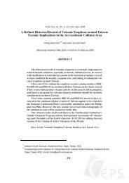
358 ß Johnson and Helferty: SIDE-SCAN SONAR 28, 4 / REVIEWS OF GEOPHYSICS 

the appropriate instrumentation has resulted in the A further major advantage of side-scan sonar is that it 

development of side-scan sonar into a new "swath can produce spatially correct data that can be viewed as an 

mapping" tool (Figure 1), one that can map the physical image. The resulting "image" is a familiar photographlike 

properties of the surface of the seafloor, and do it quickly, representation (Figure 2) that can be enhanced, modified, 

cheaply, and over a wide area [Tucker, 1966; Edgerton, and ultimately interpreted, much as a land geologist 

1966; Fleming, 1976; Mudie et al., 1970; Klein and interprets the structure of a roadside rock outcrop or an 

Edgerton, 1968; Andrews and Humphrey, 1980; Laughton, aerial photograph. The value of this ability to visually 

1981; Reut et al., 1985]. 

interpret large amounts of data as recognizable images is 

not lost on anyone who has, for example, studied multichannel 

seismic records or has been disoriented in a 

labyrinth of potential field contour lines. While side-scan 

sonar as a technique has not yet achieved the full potential 

of the initial promise, it is not an exaggeration to say that it 

has radically changed our perception of the seafloor and 

our understanding of the geological processes at work 

0 km 

Figure 1. GLORIA image from the Washington margin, showing 

two anticlinal hills at 2000 m depth. Bright pixels are hard 

acoustic returns, and dark pixels are soft returns or acoustic shadows 

(the traditional GLORIA polarity). The bright pixels on the 

left flank of the hill on the right-hand portion of the image are returns 

due to proposed carbonate deposits associated with the 

dewatering of sediments during subduction. The anticlinal hill in 

the lower left of the image is of similar topographic relief but 

does not show comparable bright reflections. (Data from U.S. 

Geological Survey.) 

there. 

The development of side-scan sonar has evolved to the 

point where we can now view these acoustic data as 

spatially correct images. These digital image data are 

"correct" in the sense that all of the acoustic targets are in 

the same undistorted spatial relationship to each other as 

they are on the seafloor. A series of mathematical 

operations can subsequently be applied to the image to 

increase our ability to interpret the data in terms of 

geological processes; the operations which accomplish this 

are grouped into the general category called "image 

processing." Basic digital processing techniques for 

optical images have been in existence since the early 1960s 

[Andrews, 1968; Campbell, 1974; Rosenfeld, 1976; 

Rosenfeld and Kak, 1976]; however, application of these 

standard image processing techniques to acoustic images 

of the seafloor is a relatively new phenomenon. With the 

recent application of digital processing to acoustic 

side-scan data, we have moved to what was state-of-the-art 

for optical images about 25 years ago. 

The direct transfer of digital image-processing techniques 

from optical to acoustic images suffers from several 

inherent problems. First, unlike the customary multifrequency 

optical images, where color conveys a tremendous 

Figure 2. SeaMARC 150 side-scan 

image of a PB4Y aircraft at the bottom 

of Lake Washington (Seattle, 

Washington). Swath width for this 

image was 100 m, and the grid lines 

are 10 m apart; water depth is 27 m. 

The starboard wing is estimated to 

be 5 m above the lake bottom, causing 

the apparent image distortion, 

and the port wing is partially buried. 

Polarity of this image is the same as 

in Figure 1. (Data from J. Kosalos.)

28, 4/REVIEWS OF GEOPHYSICS Johnson and Helferty: SIDE-SCAN SONAR ß 359 

amount of information, side-scan images are mono- nautical mile in diameter (1 nautical mile = 1.852 km). 

chromatic and, at best, consist of a small number of shades The entire acoustic return is integrated to a single data 

of grey. Second, the acoustic images are orders of point, the "depth," clearly a low-resolution image of the 

magnitude lower in resolution than those we are accus- seafloor. 

tomed to observing visually. Finally, and perhaps more Side-scan sonar, on the other hand, uses multiple, 

important, the side-scan image is not a representation of interconnected transducers rather than a single, dualhow 

the seafloor would look if the water were somehow purpose transducer used on the wide-beam echo sounder 

removed from the ocean. Instead, it is a graphical [Belderson et al., 1972]. With side-scan, a linear array of 

presentation of how the seafloor interacts with acoustic transducers (usually, the same set is used both to transmit 

energy. This conversion, from how the seafloor "sounds" and to receive) is mounted on each lateral face of the 

to how our geological models tell us the seafloor should towing body, and these transducers listen, or "scan" 

"look," can be a major pitfall for the interpreter of the outward toward either "side" of the ship track. This long, 

images. 

narrow array of transducers produces an acoustic beam that 

is wide in the across-track direction and narrow in the 

along-track direction (Figure 3b). Figures 3a and 3b show 

FUNDAMENTALS OF SIDE-SCAN SONAR 

the fundamental differences in the beam pattern between a 

WIDE BEAM ECHO SOUNDER 

Side-scan sonar is a logical extension of the same basic 

acoustic principles used in the wide-beam echo sounder 

(Figure 3a). The echo sounder has served marine geology 

well since its development in the early 1920s [Vogt and 

Tucholke, 1986; Urick, 1983]. The basic echo sounder 

consists of (1) a transmitter, which emits sound downward 

into the water column, (2) a receiver, which detects the 

reflected acoustic energy, and (3) a clock, which measures 

the elapsed time between transmitted and received pulses. 

Although there are many refinements to this basic 

procedure, these three components are the heart of the echo 

sounder and of any side-scan sonar system. The widebeam 

echo sounder emits (and subsequently listens, 

usually with the same transducer) in a roughly 30 ø wide 

cone. This wide cone intersects the bottom with a Figure 3a. Schematic diagram showing the large area of the 

"footprint" that is almost (in 3500 m of water depth) a 

seafloor ensonified with the low-resolution, 30 ø cone of the 

wide-beam echo sounder. As discussed in the text, the diameter 

of the cone at 3500 m water depth can be as large as 1 nautical 

NARROW-BEAM SIDE-SCAN SONAR mile (1.85 km). 

2 ø , so the along-track angle is greatly exaggerated. An actual 

Figure 3b. Schematic diagram (not to scale) of the acoustic 

"footprint" of a side-scan sonar system. As in Figure 3a, the beam pattern for a "real" side-scan system has many minor lobes 

grey hatched area represents the intersection of the beam pattern in all three spatial directions, and the pattern shown in this figure 

with the seafloor. Typical beam width for side-scan systems is is to illustrate the basic principles.


o _--- 

Previous Ping 

This Ping 

z 

Time 

'


mitted energy is reflected away from the transducers and limit our discussion to those features directly applicable to 

the side-scan transducers and does not reappear during the side-scan images of the deep seafloor. 

receive portion of the cycle. Only those areas of the Reflection of. sound from the seafloor is straightforward 

seafloor that have both a bottom roughness of the appropri- to understand, but it is not the dominant process in 

ate scale and an acoustic impedance (defined as the prod- side-scan returns. If the reflecting surface of the seafloor 

uct of density and sound velocity) significantly different shown in Figure 5 were entirely flat (on all scales), then 

from seawater will produce substantial backscattered en- little energy would actually be returned to the transducers. 

ergy at the receiver. With a side-scan sonar pulse (Figure Fortunately, the seafloor is rarely uniform or flat on the 

5), the effective acoustic return at the receiver is a variable smallest scale, and several mechanisms ensure that sound 

combination of backscattered (diffracted) and specularly is radiated back in nonreflected directions. The small-scale 

reflected (as from "tiny" mirrors) sound from the seafloor. microtopography of the bottom material will, through 

The received side-scan signal depends mainly on the diffraction, reradiate some small fraction of the incident 

backscattered energy from the seafloor, and the strength of sound wave back in the direction of the transducers. This 

the acoustic return depends, in part, on the acoustic diffraction of sound, from features whose horizontal scale 

impedance contrast between the target and seawater. The is comparable to the acoustic wavelength, will give rise to 

amplitude of the returned signal also has a further depend- a measurable backscatter signal. Where there is little 

ency on the angle of ensonification: the angle of incidence penetration of the acoustic energy into the seafloor (i.e., a 

between the sound wave front and the surface of the basalt flow), this surface reverberation is the major source 

seafloor. This angle in turn depends on the slope of the of returned energy detected at the side-scan transducers. 

bottom and the position of the tow body, or "fish." There The efficiency of this backscatter process is not high, 

are several different scales of bottom topography to with the bulk of the acoustic energy being reflected away 

consider, the most obvious two are the regional slope, from the side-scan transducers. It can be seen intuitively 

which is generally much larger than the wavelength of the that the amount of energy backscattered by this mechanism 

incident sound, and the microtopography, that scale of depends on the roughness of the material on the seafloor. 

surface roughness that is smaller than the wavelength of Materials which have a rougher surface will backscatter 

the incident sound (Figure 5). Many excellent acoustics energy more efficiently (with a higher amplitude return at 

texts discuss the physics of the interaction of sound with the side-scan receiver) than smooth materials with the 

the seafloor (see, for example, Urick [1983]), and we will same acoustic impedance contrast. 

backscatter 

! 

! 

! 

! 

! 

øt I 

,' reflected energy 

combines with beyond the 

P'I Vt strong echo on backscatter 

P2V 

slopes limit 

Figure 5. Diagram showing the fate of an outgoing acoustic shown, the backscatter limit, beyond which there are no useful 

pulse as it interacts with the seafloor. Within the effective range returns, can depend on the regional topography. The amplitude 

of the side-scan the returned acoustic energy is a combination of of the backscattered return, as discussed in the text, depends on 

backscattered energy and specular reflection, with only a small the acoustic impedance contrast (density times sound velocity of 

amount of direct planar reflection energy from the seafloor. As each material) between the seafloor and the overlying water.

362 ß Johnson and Helfert¾: SIDE-SCAN SONAR 28, 4/REVIEWS OF GEOPHYSICS 

For the interpreter of the side-scan image, the slight Figure 4 shows a schematic diagram of the entire 

difference in textures presented by the microreflectivity of side-scan process that begins with the initial ensonification 

the seafloor surface (Figure 5) is all the information that is of the seafloor and ends with the generation of an acoustic 

available. The appropriate choice of side-scan frequency image. At the initiation of a side-scan cycle, the transducer 

should be to try to match, as closely as possible, the array generates an outgoing acoustic pulse, usually a short, 

wavelength of the sonar with the appropriate scale of the continuous tone of a single frequency. The GLORIA II 

roughness of the seafloor, assuming it is known a priori. system uses a frequency-modulated (FM) pulse, but that is 

This frequency choice must be consistent with the other the exception rather than the rule for side-scan systems 

goals of the survey, because high-frequency sound usually [Tyce, 1986]. The length of the pulse of the outgoing 

means slow, near-bottom towing, coupled with the smaller sound energy is an important factor in determining the 

spatial coverage associated with the resulting narrow swath ultimate resolution, with shorter pulse lengths giving 

widths. 

higher resolution, for a given set of system parameters. As 

In regions where there is substantial sediment on the a trade-off with resolution, longer pulse lengths contain 

seafloor, surface microreflectivity does not contribute as fewer frequencies than shorter pulses, are therefore easier 

much backscatter energy as volume reverberation [Tyce, to filter for noise, and also contain more acoustic energy 

1976; Fox and Hayes, 1985; Jackson et al., 1986]. per pulse. The easier detection of these longer and more 

Significant deep-sea sediment penetration of sound occurs energetic pulses can increase the working swath width of 

at frequencies of 12 kHz or lower, and in this case, a the side-scan system. Typical pulse lengths range from 

phenomenon called volume reverberation takes place. 2-4 s for the long-range GLORIA II signal to less than 0.1 

During this process, sound penetrates below the surface of ms for the high-frequency (>100 kHz) systems. 

the water-sediment interface, interacts with a volume of the During the transmit pulse, the receiving circuitry of the 

sediments, and then is effectively reradiated in all direc- side-scan is switched off, to prevent damage or saturation 

tions, including back in the direction of the side-scan of the high-sensitivity amplifiers. After the completion of 

transducers [Stanton, 1984; Jackson et al., 1986]. The the transmit pulse, the transducers are switched over to the 

depth of acoustic penetration, and therefore the amount of receiving circuitry, and the continuous recording of the 

subsurface sediment that is involved in the reradiation of incoming acoustic signal begins. As the outgoing sound 

the sound, depends on the frequency of the sound and the pulse travels through the water column, the acoustic energy 

physical properties of the sediments. Accordingly, encounters only midwater scattering sources (i.e., fish, 

low-frequency acoustic side-scan images contain more, or temperature/velocity inversions, and particulate matter), 

at least different, information about the bulk properties of which normally register little energy at the receiving 

the sediments that make up the seafloor than those transducers. When the bottom reflection arrives at the fish, 

obtained with high-frequency instruments. 

this signal starts the high-resolution timing function that 

controls the generation of the side-scan data (Figure 4). 

After the bottom return arrives at the transducers, it is 

ANATOMY OF A SINGLE SIDE-SCAN SONAR PING followed by acoustic returns from the seafloor at increasing 

distances from the ship track. Being a direct reflection, 

The combined directivity of the multiple transducers in the "bottom bounce" is invariably a very strong return. 

the side-scan array results in a narrow wedge-shaped Because of the near-vertical incidence of the sound wave 

footprint on the seafloor (Figure 3b), one that is narrow front as it impinges on those areas immediately below the 

along track and very extended in the direction per- ship (Figure 4), the sampling rate of the pixel generator 

pendicular to the ship track. This narrow strip can be (the device that divides the time scale into individual time 

thought of as two parallel time lines, one on each side of slices) would need to be too high (almost infinite for 

the ship, with the earliest acoustic return being from the near-vertical incidence) to be achieved practically. The net 

seafloor that is directly under the ship (T = 0) and the latest result is that the region of the seafloor directly under the 

time occurring when the sound arrives from the distal side-scan tow body cannot be used in the acoustic image. 

flanks on either side of the beam pattern. These time lines Most systems automatically eliminate these ne-nadir 

can be electronically subdivided, and each time slice acoustic returns from the data set. These usually consist of 

treated as an individual "beam," thus forming multiple the innermost 40 pixels out of 2048, or about 2% of the 

acoustic beams from what is, in reality, the seafloor total image. For the GLORIA II system, this amounts to a 

response to a single "ping." Although Figure 4 represents linear distance of about 1200 m, out of a total swath width 

the entire beam pattern as a single entity, in actual practice, of 60 km [Reed, 1987; Tyce, 1986]. 

each side of the track line is ensoniœied with its own set of Once the initial "spike" of the high-amplitude bottom 

transducers, and at distinct frequencies, so that there is no bounce is suppressed, the side-scan processor begins to 

interaction between the two sides. As an example, the divide the transducer voltage time series, which is 

GLORIA II side-scan instrument uses a frequency of 6.2 produced by the subsequent bottom return signals, into 

kHz on the port side and 6.8 kHz on the starboard side unequally spaced "time slices." Because of the geometric 

[Somers et al., 1978]. 

effect illustrated in Figure 4, these time slices are ex-


tremely narrow for the early returns and much wider for it moves away from the transmitter (and also as the 

the later returns from a more distant slant range. Within backscattered energy transits from the seafloor back to the 

each time slice, the varying voltage of the transducer receiver). For a spherical wave, this reduction in intensity 

represents the acoustic energy backscattered from a fairly varies as the inverse square of the distance to the target. 

large area of the seafloor, an area much larger than that For the two-way travel of the narrow side-scan acoustic 

represented by the pixel size on the final image. The beam, this spreading loss is a complex function of the 

voltage within each individual time slice is averaged beam width and is usually determined empirically. 

(Figure 4) and then converted to a single digital number Seawater, like any other medium that transmits waves, also 

that is assigned to a specific pixel location. In practice, the absorbs energy from the sound, decreasing the amplitude 

conversion from uncorrected transducer voltage to of the wave. In salt water, this sound absorption is due 

spatially correct pixel values is more complicated than this largely to the presence of dissolved magnesium sulfate 

description. The process varies significantly from system and, to a lesser extent, boric acid. Additional energy is lost 

to system and, as described below, requires a variety of to the wave packet owing to scattering within the water 

additional corrections to become an intelligible image. column by small suspended particles, bubbles, and 

Modem side-scan systems now digitize the output of the occasionally fish and other organisms. 

receiver and spatially correct the data further so that they All of these losses can be corrected by application of a 

more closely represent a recognizable image [Blackington time-varying gain (TVG) to the returned signal. This TVG 

et al., 1983; Hussong et al., 1985]. 

is an amplifier which has a gain that increases nonlinearly 

with time after the start of a side-scan cycle. Figure 6 

Preprocessing of the Data 

shows a hypothetical signal amplitude that decreases with 

In order for the side-scan returns to become a recog- increasing time owing to the geometric, absorption, and 

nizable image, the pixels need to be corrected for a variety water column losses. Application of an appropriate TVG 

of effects. These include slant range correction (com- corrects for these losses. Since the signal level decreases 

pensating for the unequal time slice intervals), absorption of strongly with time, a covarying increase in amplification 

sound by seawater, the geometric effect of spreading (time- can produce the constant average signal level needed to 

varying gain amplification), and variable ship speed. The fi- produce a recognizable image. The TVG settings can vary 

nal product is an image that has a 1:1 aspect ratio (i.e., spatially, usually owing to water temperature conditions or 

square pixels) and one that has the sonar targets in roughly as a function of time, because of transducer "aging" or 

the same location on the chart recorder as they are on the changes in the beam shape. The appropriate TVG settings 

seafloor. The necessary corrections consist of two basic are usually determined empirically by surveying a region 

operations: putting the pixels in the "fight" place in the im- of the seafloor (usually heavily sedimented) that is 

age (the water column and slant range corrections) and giv- assumed to be absolutely featureless and adjusting the 

ing the pixels the "correct" amplitude values (the time- TVG until the displayed image appears uniformly bright. 

varying gain correction for spreading and absorption losses) A TVG setting that precisely deconvolves the signal 

[Chavez, 1986; Reed and Hussong, 1989]. 

transmission losses is rarely achieved, and this inability to 

Water column corrections are straightforward operations attain the "ideal" can be a source of serious frustration for 

that attempt to take into account the fact that most side-scan the side-scan user. 

receivers begin acquiring data immediately following the 

blanking pulse associated with the transmit part of the cycle. Image Construction 

Correcting for the time that the outgoing pulse is in the Each area of the seafloor that is within the swath of the 

water column consists simply of subtracting a constant off- acoustic beam (Figure 7) can be assigned a location in 

set in time, such that the display processor does not start the side-scan "space." This location consists of a record 

construction of the actual image until the sound from the number (one for each ping) and a pixel number (the 

bottom has arrived at the receiver. Suppression of the near- number of pixels, or distance, from the ship track in the 

nadir pixels also occurs during this part of the process. image). For most side-scan systems, there are ap- 

The slant range correction can be thought of as the proximately 1024 pixels per side, or 2048 total pixels in 

trigonometric calculation necessary to convert the actual the full swath. Associated with this location pair (the 

measured straight line (the slant range) distance of a give n record and pixel numbers) is an individual pixel value, a 

piece of seafloor through the water column (Figure 4) to a single number that is the average of the voltage that 

horizontal distance along the seafloor, from the nadir of the occurred during the relevant time slice. Depending on the 

fish to the target. Slant range corrections also compensate system, each pixel value is usually an 8-bit integer 

for the fact that equal time slice intervals do not cor- (ranging from 0 to 255, or 256 possible shades of grey), 

respond to uniform intervals of distance from the ship which represent the value of the received acoustic echo 

track and therefore do not represent true horizontal dis- after detection and after the electronic low-pass filtering 

tance intervals from the inner edge of the image. 

associated with the time slice averaging. 

The spreading correction takes into account the fact that A complete description of the side-scan record of an 

the outgoing sound pulse becomes reduced in intensity as individual region of the seafloor in the side-scan swath at


Time (or Distance) 

Time 

Constant Signal Level 

(SA) X (TVG) 

Time 

Figure 6. Application of a time-varying gain (TVG) amplification 

to a nonconstant signal. (Top) The natural decrease with 

time of a returned acoustic signal that decays because of geometric 

spreading and absorption. Since the actual signal is a rapidly 

varying function, this curve is just the upper envelope of the 

amplitude curve. If this side-scan signal were displayed without 

correction, the image would be too strong in the near-fish returns 

and too weak in the far-field returns. (Middle) The systematic increase 

in amplification of the TVG. The increase in amplification 

with time is designed to compensate for (and deconvolve) 

the decrease in amplitude in the signal due to geometric spreading 

and absorption. (Bottom) The ideal, correct TVG applied to 

the signal. In this case the TVG exactly compensates for the signal 

losses, and the signal level presented in the image is rangeindependent. 

Backscatter amplitudes in this ideal case now depend 

on the properties of the seafloor material, not distance from 

the side-scan fish. 

this point consists of (1) the location of the ship, and 

therefore the location of the side-scan fish, in latitude and 

longitude space, (2) the record number of the ping and the 

pixel number on the image, (i.e., record 4032, pixel 0823, 

starboard side), and (3) the amplitude of the pixel value, 

generally a positive integer from 0 to 255, representing the 

relative intensity of acoustic backscatter. For shallowtoned 

systems, like MARC II and GLORIA, the ship and 

fish locations in item 1 are generally assumed to be the 

same, within the range of errors of the ship positioning 

system. For deep-towed systems used in substantial water 

depths (i.e., for the SeaMARC I, AMS, and Klein systems), 

the location of the fish with respect to the ship 

presents a major uncertainty. In these cases, because the 

fish is close to the bottom and them is substantial distance 

between them, the ship and fish locations can differ by 

several kilometers (Figure 7). This offset in location can 

change dramatically in a single track line, depending on 

the changes in the ship track. 

For item 2 a number of corrections still need to be made 

before the sonar targets are accurately located in space, and 

such corrections represent a major postcruise processing 

effort. Figure 7 also shows some of the more obvious 

difficulties that can occur in processing and interpreting 

the resulting images when the ship track is not straight, an 

ideal that is difficult to achieve in the real ocean. Devia- 

tions in the cruise track from a straight line not only add 

uncertainty to the actual fish track, but the ensonification 

pattern becomes "incomplete" on the outside of a curved 

4036 

4034 

4032 

. 4030 

Fish 

Side 

\\ Ship Track 

I 

PN=0823.. PN=1024 

Side 

Figure 7. Diagram showing the registration of data in a horizontal 

plane of "side-scan space." Each data point, or pixel value, is 

uniquely identified by a record number (one for each ping) and a 

pixel number (generally 1024 pixels on each side). This diagram 

also shows the difficulty in the spatial registration of data on a 

real, nonstraight track line and the incomplete and redundant coverage 

that results on the outside and inside of tums.

28, 4 / REVIEWS OF GEOPHYSICS Johnson and Helferty: SIDE-SCAN SONAR ß 365 

track line, while at the same time it oversamples the area 

on the inside of the turn. 

adversely affect side-scan images have been recognized 

[Belderson et al., 1972; Tyce, 1986; Chavez, 1986; Reed, 

Finally, the relative amplitude of the individual pixels 1987; Reed and Hussong, 1989]. Reed and Hussong 

[1989], for example, describe an elegY'ant "backgroUnd 

contains all of the geological information in the side-scan 

record. These pixel numbers are only relative values and subtraction" technique that corrects for many of the system 

have meaning only with respect to each other. Within a artifacts that are generated in the image. These artifacts 

given side-scan system, the amplitude signals that become include bottom and surface "echos" (acOustic energy that 

pixel values are dealt with consistently, which makes arrives at the transducers after multiple reflections from 

spatial comparison within and between individual swaths these surfaces), incorrect bottom detections, and nonpossible. 

The uncalibrated nature of the transducer output, uniformities in the beam pattern. The technique of Reed 

however, seriously limits the ability to make quantitative and Hussong [1989] calculates the mean and standard 

comparisons between side-scan systems, even over the deviation of along-track swath data over a large portion of 

same regions of the seafloor. 

the image (outside the region where there are artifacts) and 

To account for the variations in ship speed that occur in then uses these "expected" values to modify the image 

a "real" survey, each image that is displayed needs some where there are artifacts in the data. While successful in 

correction factor to provide a proper aspect ratio. The removing known artifacts from the data, this background 

correct aspect ratio is one where the distance represented in subtraction technique is a fundamental modification to the 

the image in the X direction is the same as that in the Y image data and may make between-image comparisons 

direction, a ratio of 1:1. In side-scan images, this is done 

by controlling the number of repeated lines that are added 

difficult. 

to the image after each data line. Each side-scan cycle Bottom Slope Corrections 

consists of an initial "ping" followed by a stream of data Regional, or large-scale, slope of the seafloor in the area 

that represents a time-sequence of returns at increasing of a side-scan survey can play an important role in the 

distance from the ship track. If these time series data were appearance of an image, an effect that can require both 

simply presented "as is," without any correction for ship geometric and radiometric corrections. Bottom slope or 

speed, the resulting image would appear extremely topography can modulate both the amplitude of the return, 

compressed and distorted in the along-track direction. at the pixel level, and the apparent texture of the seafloor 

In order to provide the necessary speed correction and acoustic targets, at the image level. Radiometric correcthe 

ability to view pixels that are "square" in aspect ratio, tions that alter the pixel values of targets located on inward 

image display programs insert duplicate lines after the and outward facing slopes must be applied to allow a 

initial data line, with the number of repeated lines propor- spatially correct interpretation. Large-scale regional 

tional to the ship speed. Largely because of the historical changes in the slope of the seafloor can induce substantial 

use of shipboard graphic recorders, most imaging systems geometric errors in the actual location of acoustic targets 

add a single duplicate line for each knot of ship speed (1 within the image. Reed and Hussong [1989] discuss this 

knot = 1.85 km/h). As an example, side-scan data taken at "layover error" at some length, and Reed [1987] provides a 

7 knots are normally viewed as one data line and six fortran program which can correct for the effects of this 

repeated duplicates of that line. Because only integer error. While the effects of (and remedies for) the layover 

multiples of the data lines are possible (either six or seven correction are adequately described in the literature, it is 

repeat lines can be added, not 6.5), it is not possible to probably useful to review the causes of the phenomenon, 

correct for speed variations smaller than 1 knot. This is a to be able to estimate the magnitude of the effect, and to be 

limitation to our ability to spatially correct the data that is able to apply the correction to the data "by hand" if 

significant only for slow speed, near-bottom systems. This 

replication of the data lines does not change resolution or 

necessary. 

the image processing functions, but is only an artifact of Layover Correction 

the display process. 

One of the basic assumptions that is made in the 

processing of side-scan data is that the seafloor is both flat 

POSTPROCESSING CORRECTIONS TO TH E DATA 

and horizontal (Figure 8). To the extent that this assumption 

is not true, and the real bottom is uneven and slopes, 

an error in across-track position is introduced in the 

In addition to real-time shipboard data manipulations, placement of the acoustic targets. To the geologist, 

postprocessing corrections are usually applied to side-scan uneven seafloor is interesting geology, and small-scale 

sonar data. These postcruise modifications fall into the corrections or the topography are neither necessary nor 

same general categories as the shipboard corrections, i.e., desirable. Large-scale regional slope, like a continental 

spatial or geometric corrections, which change the location margin or seamount flank, however, can cause substantial 

of the pixel values within the image but do not change errors in the placement of acoustic targets. The qualitative 

their value, and radiometric corrections, which change the effect of this error can be described as follows: where the 

value of specific pixels. Several phenomena that can seafloor slopes up from the nadir of the side-scan fish, the


t >Uphill 

28, 4 / REVIEWS OF GEOPHYSICS Johnson and Helferty: SIDE-SCAN SONAR ß 367 

determines many of the other system parameters. Because translates the up-and-down vertical motion of the ship to a 

of the physical properties of sound waves, particularly oscillatory horizontal motion that causes less distortion to 

attenuation, these dependent parameters include towing the image. As examples of towing configurations, the 

altitude (using either a deep-towed or surface-towed SeaMARC II system is towed 50-100 m below the sea 

configuration), the below-surface depth of interaction of surface, regardless of the water depth. In contrast, the 

the backscattered sound (the penetration), and image SeaMARC 1A system is towed either at a constant depth 

resolution. While the velocity of sound in water is largely over the bottom, generally 100 m above the highest 

independent of frequency, the absorption of acoustic upward projection of the seafloor in the survey area, or in 

energy in the water column, the ability to penetrate the "draped mode," at a constant altitude of 100-200 rn 

sediments, and the practical limitations on pulse length are above the varying bottom. 

all strongly dependent on frequency. 

Surface-towed systems, with their lower frequency, can 

Strong absorption of high-frequency sound by seawater be towed faster (7-8 knots (13-15 km/h) compared with 

limits surface-towed deep-water systems to frequencies of the 1-3 knots (1.85-5.55 km/h) in the deep-tow mode) 

less than 30 kHz. Side-scan frequencies currently in use in and have a wider swath width (40-60 km for GLORIA, 

the open ocean range from the 6-kHz (GLORIA II) and compared with 1 km or less for the deep-towed systems). 

12-kHz (SeaMARC II) instruments used by surface-towed As a practical rule-of-thumb, swath widths and tow-fish 

systems, to the 30-kHz (SeaMARC I) and 110- to 150-kHz altitudes are roughly related by a factor of 10; a 1-km-wide 

(Scripps Deep-Tow, AMS-120, SeaMARC 150, Klein) swath SeaMARC 1A survey would normally be flown at 

instruments used in deep-towed systems. Existing an altitude of 100-200 m. Technical comparisons of the 

side-scan sonar systems are deployed in a "fish," towed properties of different side-scan systems are abundant in 

behind the hull of the surface ship. In addition to system the literature, with good reviews by Tyce [1986], Davis et 

portability, this configuration is used to decouple the 

transducers from the motion of the ship, to reduce the 

amount of ship-generated noise at the receivers, and, most 

al. [1986], Mazel [1985], and Chavez [1986]. 

important, to get below the strong velocity gradients RESOLUTION 

associated with the thermocline in the surface waters. 

Resolution in an image is the ability to distinguish 

Towing Altitude 

closely spaced objects as individual features. In side-scan 

Figure 9 shows the basic towing configuration of a sonar images, there are several different types of "resoluside-scan 

system; this figure is very schematic but tion" that must be considered in the interpretation of the 

generally represents existing deep- and surface-towed image. As the sonar beam pattern differs fundamentally in 

systems. In this representation, the fish is attached to the the along- and across-track directions, side-scan images are 

ship through an armored coaxial cable that provides both intrinsically anisotropic. It is therefore necessary to 

the strength member for towing and the necessary understand the concept of resolution in both the along- and 

electrical connection to the surface ship. Power and across-track directions before attempting to interpret the 

control signals are sent down the cable; side-scan and geological features in an image. As an additional comtelemetry 

(altitude, pitch, yaw, depth) signals are sent up. plication, this "directionally sensitive" instrumental 

The neutrally buoyant fish is attached to the towing cable resolution is further modified in the final display by the 

through a depressor weight, a heavy mass that effectively finite pixel size of the displayed image. This range- 

Tow cable winch 

Ym 

Neutrally 

(not to scale) j=buoyant tether ( I 

Figure 9. General configuration of the towing systems used for 

side-scan sonar systems. As described in the text, the heavy 

depressor weight (1000-2000 kg) decouples the side-scan fish 

from the motion of the ship and converts the vertical wave mo- 

Depressor weight 

Slightly positively 

buoyant tow body 

tion into horizontal variations in the towing speed. Values for X 

and Y depend on the system used and can vary from several hundreds 

of meters for surface-towed systems to several kilometers 

for deep-towed systems.


independent pixel size is calculated for a given side-scan tion, but once the optimum ping rate is reached, a further 

system from the ratio of the swath width to the number of increased rate only provides more redundant data. As a 

pixels in the image, a value suitably termed the "display practical rule-of-thumb, along-track resolution is usually 

resolution." An appreciation of how the instrumental much worse than the across-track resolution [Tyce, 1986]. 

resolution and display resolution interact will allow users In the along-track direction, a fundamental control on 

both to design appropriate survey strategies and to better reSOlution is the ping rate. Two physically distinct objects 

evaluate acoustic target identification in the final images. cannot be distinguished in the along-track direction if they 

are detected only by a single ping. Individual detection of 

Across-Track ResolutiOn 

the two objects by two adjacent pings is a minimum 

Three factors control the ability to resolve sonar targets criterion. If we make the assumption that only one ping 

in the across-track direction: pulse length, the width of the should be in the water column during a single side-scan 

acoustic beam in the along-track direction and, indirectly, cycle, then we can estimate the maximum ping rate that 

the range or distance from the track line. Independent of can be used for a particular type of side-scan. Using 

their range, two targets are theoretically resolvable if their SeaMARC II as an example, with a swath width of 5 km 

separation is one-half the length of the incident sound on a side, the time required for the sound to travel the full 

pulse multiplied by the sound velocity. For the SeaMARC 10-km roundtrip distance is approximately 7 s. This is a 

II system, for example, this theoretical limit is ap- basic upper limit to the ping rate for this system and one 

proximately 7 m. In practice, the effective resolving power that is dependent solely on the desired swath width. In 

of the system will always be worse than this. The actual actual practice, SeaMARC II uses a ping rate with a 10-s 

projection of the sound wave on the seafloor increases in interval. 

width at greater distances from the tow fish (Figure 10). Because the distance traveled by the fish between pings 

This dependence of the footprint size on the distance from is a fundamental limitation for along-track resolution, this 

the side-scan fish, in the across-track direction, will be parameter is of interest and is easy to calculate. Taking 

important in our discussion of ultimate system resolution. SeaMARC II as an example and assuming a survey speed 

.15Km 

5 (m 

Figure 10. Greatly exaggerated diagram of 

the butterfly-shaped beam pattern of the 

side-scan fish as it intersects the seafloor at 

increasing distance from the fish. In this 

hypothetical illustration for SeaMARC II, the 

2 ø wide beam intersects a linear distance of 

34 m at a slant range of 1 km, and 175 m at 

the full 5-km half-width of the swath. The 

upper diagram shows the pattern of overlap 

between two adjacent pings which must be 

considered in determining the along-track 

resolution for any system. None of the dimensions 

in this figure are to scale. 

Along-Track Resolution 

of 7 knots (13 km/h) and a ping rate interval of 10 s, this 

Resolution in the direction parallel to the ship track will means that the ship travels 36 m along the track line in the 

depend largely on the width of the acoustic beam but will interval between pings. This is the ultimate limit on the 

also depend on fish height and a combination of theping along-track resolving power of the system, but, as we will 

rate and towing speed. Like across-track resolution, see, even this level of resolution is not reached in practice. 

distance from the ship track determines the ability to The horizontal angle of the acoustic beam is small but 

resolve distinct targets which are aligned parallel to the still finite, and therefore the width of the beam in the 

track line. Since the two sides bounding the acoustic beam along-track direction is not constant but spreads with 

are not parallel, the beam spreads with increasing distance, increasing dislance from the ship. This expansion of the 

and the ability of the side-scan to separate sonar targets beam with increasing distance from the track line causes a 

decreases further from the tow fish. Faster ping rates and changing footprint in the along-track direction, and the 

slower towing speeds also give better along-track resolu- changing dimension results in decreasing along-track

28, 4 / REVIEWS OF GEOPHYSICS 

Display Resolution 

The along- and across-track resolution described above 

provide the fundamental limitations to the resolving power 

of side-scan systems. Unfortunately, none of these 

inherent limits on the resolution of the side-scan system 

have any real meaning for the interpreter until the data set 

is presented as an image. The technique used to create and 

display the image which is actually viewed acts as a "final 

filter" to the data, a filter that can integrate, modify, 

artificially enhance, or (more commonly) blur the final 

image. The final image that is displayed can never be 

made sharper than the resolution limits described above 

and can be substantially worse. 

In side-scan sonar the most common form of resolution 

used is that of pixel size, the figure obtained by simply 

dividing the distance of the full swath width by the total 

number of pixels. In the SeaMARC II example this is 4.9 

m (10 km/2048 pixels). This figure has been labeled 

"image processing resolution" [Tyce, 1986] and is in easy 

Johnson and Helferty: SIDE-SCAN SONAR ß 369 

resolution. This can be seen intuitively with simple "figure-of-merit" value to calculate for the comparison of 

trigonometric arguments (Figure 10). This simple different side-scan systems. Although correctly described 

geometric expansion of a beam pattern of finite angular by Tyce [1986], this range-independent figure is frequently 

width results in a range-dependent along-track resolution misinterpreted as the actual instrument resolving power of 

similar to that previously discussed for the across-track side-scan systems. While it has the correct dimensions 

resolution. 

(length) associated with resolution, and it is certainly a 

characteristic length in the image, this value is not a true 

measure of the resolving power of the technique. In 

contrast, actual instrumental resolution must take into 

account the area of the seafloor that is the source of the 

acoustic return that is ultimately integrated into a given 

pixel. For lack of a better term, we call this concept the 

"pixel ensonification area." Since both along- and 

across-track resolution vary with distance from the ship 

track, it is also necessary to consider the range dependency 

of that area of ensonification. 

Instrumental Resolution 

Figure 11 shows a representation of areas of the seafloor 

that provide the total integrated acoustic energy that is 

averaged into a single pixel, for several different dislances 

from the track line. This diagram, modified from Karlin 

and Johnson [1987], is based on the calculations for a 

SeaMARC II system by Kosalos and Chayes [1983]. As 

shown in this figure, all of the backscattered sound that is 

received from the shaded area is averaged into the single 

.... ACROSS TRACK 

/ 6m 

/ / 

/ PIXEL NUMBER /' 

50 50 400 000 

250m 750m 2000m 5Om 

RANGE (log scole) 

Figure 11. Diagram showing the size and shape of the areas of the seafloor that are integrated into 

a single pixel value as a function of across-track distance from the fish. This figure uses 

SeaMARC II as an example and is based on the calculations of Kosalos and Chayes [1983]. As 

with Figure 10, none of the dimensions in this figure are to scale. Since the size and shape of the 

area integrated into each adjacent pixel determine the ability to distinguish seafloor targets, the 

resolution power of the systems will vary directly as the areas shown. 

i/ 

/ 

/

370 ß Johnson and Helferty: SIDE-SCAN SONAR 


pixel value. If we assume a pixel size of 5 m by 5 m for subject of data redundancy, or pixel overlap. Because the 

the SeaMARC II, then in the area nearest to the track line, active ensonification region of each pixel is much larger 

pixel number 50 (out of 1024 total) contains backscattered than the pixel in the image that represents it, and the pixels 

energy from an area of seafloor that is 5 pixels by 9 pixels are (by definition) immediately adjacent to each other in 

in size, or an area that is 25 m by 44 m in actual dimen- the image, it follows that some of the area integrated for 

sions. For this example the returned acoustic energy that is one pixel will also be included in the adjacent pixels. As 

integrated into a single pixel value comes from a pixel 

ensonification area of over 1100 m 2, not the 25 m 2 (5 m x 

with resolution, the redundant areas are different for alongand 

across-track adjacent pixels. Figure 12 shows both the 

5 m) represented by the pixel size in the image. In the along- and across-track overlap for the respective pixels, 

region that is closest to the track line, the active area of again using the SeaMARC II as an example. In the 

detected and integrated acoustic return is roughly equi- across-track direction the overlap is between adjacent 

dimensional, a circumstance that is dramatically not the pixels in a given data line, for a given ping. In the 

case at the distant edge of the image. 

along-track direction the overlap is between pixels at the 

To see how this active region varies with distance from same distance from the track line (i.e., the same pixel 

the track line, Figure 11 also shows a region at the full number, for a straight track line) but for successive pings. 

5-km distance of the swath width (i.e., pixel number 1024). In the across-track mode, shown in Figure 12, there is a 

Here the pixel ensonification area that provides the great deal (89%) of redundancy in seafloor ensonification 

returned acoustic backscattermthat is ultimately integrated for adjacent pixels near the track line and very little 

into a single pixel numbermis now only 1 pixel wide overlap (10%) for pixels at the distal end of the swath 

across track but almost 20 pixels long in the along-track width. For the inner pixels the large region of overlap 

dimension. In this distal region example the total active between adjacent pixels reduces the effective resolution; 

pixel ensonification area is 588 m compared with the 25 only those acoustic targets that are represented in one 

m that the pixel represents in the image. The more distant pixel, but not in the adjacent pixel, can be resolved. 

area is not equidimensional but is elongated 20:1 in the 

along-track direction. Two intermediate areas, representing 

pixels numbers 150 and 400, are also shown in 

Figure 11 to demonstrate how actual resolution varies with 

distance from the track line. While this example is drawn 

OVERLAP 

using the SeaMARC II system, with appropriate scaling 

-i 

the same conclusions can be applied to side-scan systems 

in general. 

Clearly, the implications of the different across-track 

areas represented in Figure 11 are important in the 

ACROSS TRACK 

interpretation of side-scan images. It can be seen that the 

effective resolution for features that are distributed parallel 

89.1% 

71 .% 

37.5% 

10.5% 

to the track line is much greater at the distal edge of the 

-. 

swath than close to the center line. This figure also shows 

why some types of geological features seem to have a 

fundamental anisotrophy when they are viewed from ship 

tracks with different "look" directions. When the elongate 

areas of ensonification are parallel to the texture of the 

feature, the textures can be resolved; when the textures are 

oblique, they are unresolvable. Further, Figure 11 shows 

SHIP 

i 

, [] 

i 

, 

ALONG 

,- --, 

i 

i i 

,D, 

TRACK 

-i 

i i 

i i 

i 

the fundamental difference between "image-processing 

19.8*/. 20.2*/. 

37.4% 

resolution," or pixel size, and actual resolution. Finally, 

the elongate nature of the ensonification areas should have 

64.1ø/. 

Pixel Number an impact on how survey lines are planned; small-scale Meters 

features parallel to track lines will be visible in the image, 

while features perpendicular may not, depending on their 

size. Many survey track lines are now laid out at 45 ø to 

50 

250 

150 

750 

400 

2000 

1000 

5000 

the known strike of geological features, such as spreading Figure 12. Summary diagram showing how adjacent pixels 

centers [Davis et al., 1986; Kong et al., 1988] to compensate 

for this anisotropic resolution. 

overlap in the along- and across-track directions. In the acrosstrack 

direction the overlap is between adjacent pixel numbers; in 

the along-track direction the overlap is between subsequent 

Pixel Overlap and Redundant Data 

In discussions of resolution, consideration of the size 

and shape of the areas of active ensonification bring up the 

pings. As with Figure 11, the small squares in the middle of each 

larger square indicate the relative size of the pixel in the final image 

as compared with the actual area that is the source of the 

acoustic backscatter energy.



Clearly, overlap continues to degrade the resolving power dimensions much smaller than the footprints shown in 

of the inner pixels of the swath. The variation in across- Figure 11, are an obvious set of examples. For hightrack 

overlap for intermediate positions in the swath, at resolution side-scan systems towed near the bottom, using 

pixel numbers 150 and 400 (out of 1024) are also shown in 100-kHz frequencies and narrow swath widths, objects as 

Figure 12. 

small as a single piece of line or cable, lying on a smooth, 

Figure 12 also shows similar overlap of adjacent pixels sedimented bottom, have been detected [Mazel, 1985]. 

(due to successive pings) in the along-track direction. In Conversely, where the acoustic impedance of the sonar 

this example the range variation of the degradation of reso- target is similar to that of water (e.g., water-logged pine 

lution is the opposite of that for the across-track overlap. wood [Mazel, 1985], large, high-relief objects, such as 

The innermost pixels have an overlap of only 20%, while ships, can sometimes be virtually undetectable by the 

the adjacent pixels at the edge of the swath overlap by 

64%. Unlike most other effects on resolution, this effect 

has the most impact on the outer pixels of the swath and 

side-scan. 

the least effect on those in the inner region. This phenomenon 

has a direct impact on the appearance of the im- 

IMAGE ENHANCEMENT AND PROCESSING 

age, with images (and their shadows) appearing elongated Three distinct operations are loosely associated with the 

in the along-track direction, particularly in the far field of term "image processing" as opposed to the geometric data 

the image, distant from the ship track. By using point corrections described in the previous section. First, image 

migration techniques similar to those used in seismic data enhancement consists of those operations that make the 

processing, Reed [1987] has developed a digital correction image look "good," or at least more like what we expect. 

technique for the effects of this target elongation on the These operations make the data display more "pleasing" by 

side-scan image. 

modifying the overall appearance of the image. Some 

Reflection on the actual resolving power of side-scan examples of enhancement are the variation in amplitude 

sonar systems, as discussed above, can be a discouraging ex- gain, increasing or decreasing the contrast, and application 

ercise. Instead of the ability to resolve (for the SeaMARC II of threshold values (high- or low-pass filters) to the pixel 

example) objects with dimensions of the order of 5 m--a amplitudes. The second class of image processing, image 

capability that consideration of the pixel size alone would analysis, consists of operations which provide compact 

lead us to believe---we can, at best, only resolve objects numeric information based on the data within the image. 

that are several tens of meters in linear dimension. These processes distill the "essence" of the data in a image 

Further, this resolving power is both range-dependent and and present it in short-hand numeric form. Application of 

orientation-dependent and varies both with distance from these image analysis operations obviously does not change 

the ship track line and with the angle between the track line the appearance of the original image, and the results are 

and the texture-orientation of the feature. In extreme usually presented in a nonimage format, such as a table of 

cases, for objects with an unfavorable across-track orienta- numbers. Finally, the third category of image processing, 

tion and a location at the edge of the swath, we only have a image coding, includes results of mathematical analyses 

resolving ability of the order of 100 m. 

that are sufficiently complex to be presented as a secondary 

image of the original data. Pattern recognition 

Target Detectability 

techniques, including the "feature recognition" and image 

It is important not to confuse the concept of resolution classification techniques of Reed and Hussong [1989], fall 

with the ability to detect objects in the side-scan swath. 

Specifically, resolution is the ability to distinguish two 

separate targets on the seafloor, while detectability is the 

into this category. 

ability of an object on the seafloor to make a visible record 

on the side-scan image. This confusion arises because 

HISTOGRAM ANALYSIS 

side-scan sonar has the ability to detect objects on the A major tool in image processing that is used for both 

seafloor that are much smaller than the resolving power of enhancement and analysis is the image histogram. A 

that system, particularly in an area of low ambient histogram is simply a plot of the frequency distribution of 

backscatter. The fundamental criterion for detectability is pixels contained within an image (Figures 13a and 13b). 

different from that of resolution; if an object can provide In addition to being an easy-to-understand representation 

sufficient backscattered acoustic energy to the receiving of the range of values that exist within an image, histransducers 

and if the ambient background backscatter is tograms provide a mechanism for visualizing the statistical 

both uniform and low (to provide adequate contrast with techniques that are applied to pixel amplitude values. 

the hypothetical target), then the object can be "detected" Most of the major enhancement techniques that are applied 

as a sonar target even if it is considerably smaller in to images can be considered as specific mathematical 

dimension than the resolving power of the system. The operations on pixel amplitudes, which can be visualized as 

clear visibility in the side-scan record of small fissures, histogram changes. Thus histograms provide a quantitafault 

scarps, and cracks on the seafloor, features with tive component to what is normally a very subjective

372 ß Johnson and Helferb/: SIDE-SCAN SONAR 28, 4/REVIEWS OF GEOPHYSICS 

Figure 13a. A SeaMARC II image of a recent lava flow (dark) 

onto sediments (lighter) at the northern end of NSR segment, 

Juan de Fuca Ridge. In this image, traditional polarity convention 

is observed, with strong acoustic reflectors shown as dark 

pixels and weak returns as white. (Left) The acoustic image. 

(Right) An interpreted line drawing. In the figure, significant 

geological features are the lava flow (horizontal hatches), a lowreflectivity 

halo surrounding portions of the flow (diagonal 

hatches), several rounded and sedimented seamounts on the right 

side and lower center of the image, and both active (dark) and inactive 

(light grey lineations) faults. The direction of ensonification 

is from the left edge of the image. 

operation. Since acoustic images are monochromatic, we 

are concerned here only with what is termed as the "grey 

level histogram." 

Side-scan images are generally arrays of 8-bit numbers, 

values which represent 256 (i.e., 28 ) intensity levels, or 

shades of grey. This means that the horizontal axis of the 

histogram varies from 0 to 255, while the vertical axis 

displays the total number of pixels in each column. Figure 

13a shows a side-scan image that contains both hard 

acoustic reflectors (newly erupted basalt) and soft acoustic 

reflectors (unconsolidated sediments). The clear separation 

of the pixel amplitude distributions within each region 

illustrates the power of the histogram to define the acoustic 

reflectivity for homogcnous sonar targets (Figure 13b). 

Unfortunately, the majority of side-scan images from the 

seafloor produce much more complicated histograms, with 

pixel values distributed over the entire range of possible 

values. While extremely valuable in defining the distribution 

of pixel values, the histogram does not provide any 

information about the spatial distribution of these pixels 

within the image. 

Two additional concepts are important in any discussion 

of image enhancement: contrast and dynamic range. Both 

of these concepts can be easily interpreted in terms of pixel 

distribution within the image histogram. Image contrast 

can be defined as the "separation" of pixel values within a 

histogram: a low-contrast image has pixels narrowly 

grouped about one central value of the histogram (Figure 

14a), while a high-contrast image has a bimodal distribution 

of pixels, with the two high-density distributions 

located at opposite ends of the histogram (Figure 14b) 

Generally, an image that is pleasing to the eye has pixel 

values that are uniformly distributed throughout the 

histogram, although this may not produce the desired 

representation of specific geological features. 

The dynamic range of pixel values within an image is a 

measure of the width of the occupied portion of the 

histogram in comparison with the total number of pixel 

amplitude values available. An image with pixel values 

Maximum 255 

Minimum 2:10 

Range 46 

Mean 236 

Median 237 

Mode 238 

Maximum 255 

Minimum 59 

Range 185 

Mean t66 

Median 166 

Mode 160 

Maximum 

Minimum 

Range 

Mean 

Median 

Mode 

Area t 

Area 2 

I 

o 

A 

INTENSITY HISTOGRAM 


255 C 

o/o70 ' 


Figure 13b. Histograms of the areas marked A, B, and C in Figure 

13a. Area A is the low-reflectivity region of modified sediments 

adjacent to the recent flow, where the backscatter has been 

altered by some unknown process. Area B is the lava flow 

(which has been both dredged and photographed with a deep-tow 

camera). Area C was chosen as a region that contains both sediments 

and flows. In these diagrams, pixel amplitude value 0 is 

the strongest possible acoustic return, and 255 is essentially no 

return. 

255 

I 

255 

255


a Low Contrast Lavaflow 

on Lavaflow 

>): --½. 


pixel values throughout the full dynamic range of possible 

narrowly grouped around any specific value (Figure 14a, 

for example) is said to have a low dynamic range. Very values, by histogram sliding and/or stretching, is a 

high contrast images (Figure 14b) can also be considered technique that is often applied early in the processing 

to have low dynamic range because of their narrow (even if 

bimodal) distribution of pixel values. High dynamic range 

stage. 

images (Figure 14b) are generally considered more Histogram Sliding and Stretching 

pleasing, because they are closer in appearance to natural Histogram sliding and sixetching are two processes that 

optical images and are commonly perceived by the viewer redisixibute the pixel amplitudes over the full range 

to contain more information than low dynamic range (0-255) of possible values. While this can sometimes 

images [Baxes, 1984]. In side-scan sonar, images with a make a more pleasing and recognizable image (as can be 

low dynamic range are a common problem because of the seen in the comparison of Figures 15a, 15b, and 15c), it is 

nature of the acoustic reflectivity. Reallocation of the important to understand that the pixels redistributed during 

Meon 207. 9 

Medion 2t: > 

Mode 2t7 

Entropy 6.43789 

Stond. Oev. 22.9503! 

ß I i I' ! I I- I T 'i I' I-'"! I I I ß I I I I I I 

O 50 00 50 2OO 250 


Meon 193.5 

Medion 205 

Mode 239 

High Contrast Lavaflow 

on Sediments 

Entropy 7.16549 1[ 

i I I I I I I i I i I I I I I I I I I !' I .... !"1 I I I 

O 50 tO0 1.50 200 250 


Figure 14. Two SeaMARC II images and associated histograms appears to be only a single population of pixel values, and even 

showing examples of high and low contrast in side-scan images. with some enhancement, the flows are difficult to distinguish 

(a) Image from the southern Juan de Fuca Ridge, showing the from the background. Lava flows contrasted with sediments. 

low contrast associated with lava flows on top of only slightly The histogram of the marked area clearly shows two distinct 

older lava flows. The histogram of the marked area shows what populations of pixel values.


:*..:"5 '. 

...- :.'i 

ecn 202.8 

Mealion 214 

ode 


0 50 tO0 t50 


Figure 15a. SeaMARC II image of the same area shown in previous 

figures, but now with the histogram of the entire image 

shown. This histogram, which from the spatial relationships in 

the image has three distinct populations of pixel values, shows 

that the overlap in populations obscures any distinction. 

Meon t3t. t r E 

Median 140 I,i, 

Mode 

Entropy 6.6i874 ? 

' ['-- i i i i i i i i i i i i i i i i i i i i i i i i 

50 t00 50 200 ?.50 


Figure 15b. The same image as shown in Figure 15a, but now 

subjted to a pixel amplitude "slide" of--80 (subtracting 80 

from each pixel value), which makes the entire image darker and 

lower in contrast. 

histogram manipulation do not contain any more informa- increase both the dynamic range and the contrast of the 

tion than the original image. Histogram sliding is a image. Mathematically, a histogram "stretch" is the simple 

process that moves the "center-of-mass" of the pixel multiplication of the pixel amplitudes by a constant value, 

amplitude distribution to the middle of the range. usually, but not necessarily, an integer. If NPV and OPV 

Histogram sliding is the simple addition or subtraction of a are the new and old pixel values and K is some constant, 

constant value to all the pixels within the image. Since the then 

acceptable range (for display) for 8-bit images is within 

0-255, this operation can, for certain offsets, produce new 

NPV (n) = K x OPV (n) 

values that are outside this range. The over-ranging of the 

new image pixels is a common problem that occurs in 

image-processing operations, and simple arithmetic The effect of this multiplication is to increase (or decrease) 

operations are used to move the pixel array values back the distribution of the pixels throughout the entire range of 

within acceptable display values. 

the histogram. A "linear stretch," for example, is simply 

Similar to histogram sliding, histogram stretching is a taking the difference of the maximum (PVmax) and 

simple mathematical operation that redistributes the pixel minimum (PVmin) occupied histogram values and 

values within a histogram, an operation generally done to dividing each old pixel value by the factor that expands the

28 4/REVIEWS OF GEOPHYSICS Johnson and Helferty: SIDE-SCAN SONAR ß 375 

Mean ' t0t.0 6 C 

Median'' t07 / t 

Mode t15 / 1 


Histogram Equalization 

Histogram sliding and stretching are usually operations 

that are performed together, as a combined operation called 

"equalization," to manipulate the pixel distribution for a 

more recognizable image. In practice, this operation is a 

histogram modification procedure that assigns equal 

numbers of pixel values to each of the divisions in the new 

image. This operation can be thought of as a mapping 

process between the old pixel values of the original image 

and the modified values of the new image (Figure 16). 

The process of equalization adjusts the new pixel value 

assignments such that there are an equal number of pixels 

with each new amplitude value. For example, if there were 

a total of 1600 pixels in the original image and 16 grey 

scale levels (pixel amplitudes) that could be displayed, 

histogram equalization would assign an "equal" number, 

100 pixels in this case, to each of the individual grey scales 

in the new image. The effect of equalization is to expand 

the contrast between grey levels that occur frequently and 

to decrease the contrast between those pixel amplitudes 

that occur infrequently, using the limited amount of 

available image contrast where it is most effective. The 

mathematical operations necessary to perform image 

equalization are described by Pratt [1978], and the 

appropriate algorithms to accomplish it with acoustic 

images are developed by Reed [ 1987]. 

FILTERING 

ß 

Spatial filtering can be generally defined as that analytit 

I I I I I I i 

cal process that separates the individual frequency compo- 

50 too ! 50 

INTENSITY HISTOGR/M 

200 250 

nents of an image, where the term "spatial frequency" is 

used to describe the variation in relative amplitude values 

Figure 15c. The same image as shown in Figures 15a and 15b, 

but now subjected to a pixel amplitude "stretch" of 0.5 (dividing 

the pixel amplitudes by 2, which is actually a histogram compression). 

Again, the image becomes darker and much lower in contrast. 

These operations do not, obviously, improve the image and 

of adjacent pixels. A region of an image in which adjacent 

pixels have widely varying values is said to have high spatial 

frequency components, while an image with relatively 

little local variation is said to have low spatial frequency 

components. Filtering, or convolution, is the most comare 

shown as examples of specific histogram manipulations. His- mon procedure used in image enhancement. It is an operatogram 

equalization, which is a combination of sliding and tion typically applied to the image to produce such effects 

stretching, is the operation normally done for image enhancement as smoothing (the removal of high-frequency noise) or 

in the initial stages of processing. 

edge detection (the emphasis of specific linear features). 

Many of the operations thought of as general "image 

distribution to fill the entire range. Computationally processing" are, in fact, simply applications of different 

[Pratt, 1978; Reed, 1987], the new pixel values can be types of filters. 

generated by 

A filter can be described by a two-dimensional array of 

numbers, known as the "kemel." In general, kemels are 

NPV = [(OPV - PVmin)/(PVmax - PVmin)] x 255 equidimensional, and typical sizes for filters are 3x3, 5x5, 

and 7x7, although any dimensions may be used, and there is 

As with histogram sliding, histogram stretching can also no real requirement for filters to be the same size in both 

produce pixels that are outside the range of values (0-255) directions. Convolution is a signal-processing operation that 

acceptable for display. While the stretching operation ' combines two signals to produce a third array of values. In 

almost always improves the appearance of low-contrast, image processing, one of these signals may be the original 

small dynamic range images, exactly the same amount of image army, and the other is the filter matrix. The filtering, 

information is contained in the new image as was in the or convolution process, involves sequentially replacing each 

old. cell (or pixel) of the image with the dot product of the kernel


Default Values 

I ! I I I I [ I '[' I i --1---'!-- I [ i i I ! i I I I I l 

0 0 tO0 t50 200 250 



Equalized 


t 25 50 7,5 100 225 

Figure 16. Application of histogram equalization to a using the area shown in the boxes, the image becomes higher in 

SeaMARC II image east of Axial Seamount on the central Juan 

contrast and much easier to interpret. In the histograms below 

de Fuca Ridge. The image is low in dynamic range and contrast, the images, only the scale on the right-hand diagram is changed. 

and it is difficult to distinguish off-axis lava flows even on top of This is to illustrate the equalization process that places equal 

a turbidire sediment background. After histogram equalization, numbers of pixels in each grey-scale level. 

and the pixel's neighborhood values (Figure 17). To illustrate 

this, consider the general 3x3 filter: 

F=def 

[abc 

ght] 

To apply this filter to an image, we replace each pixel 

l(x,y) of the image as follows: 

l(x,y) = l(x - 1, y - 1)*a + l(x, y-1)*b + l(x + 1, y - 1)*c 

+ l(x - 1, y )*d + (x,y )*e + l(x + 1, y ),f 

+ l(x - 1, y + 1),g + l(x,y + 1),h + l(x + 1, y + 1) *i


Note that for two signals, one of size N and the other of 

size M, the output signal has size N + M. 

It is also useful to note that this filtering operation is a 

straightforward process until the edge of the image is 

reached, where there are no pixels "adjacent" to those on 

the outer boundary. This effect causes degradation around 

the margin of a filtered image, an effect which can be 

lessened by adding artificial data outside the original 

image boundary. 


The following filter is a simple 3x3 smoothing filter. 

[1 1 1 

F= 1 1 1 

Applying this filter to an image (Figure 18) causes each 

cell to be replaced by the sum of the cell and its eight 

immediate neighbors. This is essentially computing the 

SPECIFIC FILTERS AND ANALYTICAL TECHNIQUES mean of the pixels within the kernel and placing that mean 

in the pixel location of the central value. This filtering 

Low-Pass (Smoothing) Filter 

process will eliminate any large local variations in pixel 

A low-pass filter (or smoothing filter) removes high- value and produce a "smoothed" image. The primary 

frequency variations in an image. This technique can be disadvantages of the above technique are the "blurring" of 

used to remove the "grainy" or "snowy" texture in noisy sharp features within the image and the loss of dynamic 

side-scan images and is a useful first step in image range. This loss of information can be reduced by 

enhancement. Low-pass filters come in many forms. In weighting the filter such that the central cell values have 

the simplest case, all kernel values are equal. 

more influence on the result than distant cells. 

I 

Oric. inal Image 

,a b c 

d e f 

g h i 

- KERNEL 

Filtered Image 

Mapping 

Function 

Figure 17. Schematic of the operations associated with filtering. 

In a normal 3 x 3 filtering operation the pixel values in an image 

array are convolved with the kernel values in a 3 x 3 mask. In 

the upper diagram a 3 x 3 filter mask with values a through i is 

placed over a portion of the image. The pixel value in each image 

cell is multiplied by the corresponding value of the filter. 

The sum of these products (7 in this example) is mapped into the 

center of the filtered image in the lower diagram. 

ß 

ß -., .:,.,/.:, 

½'./!..-' 7. ;3. 

..:.::.... :_,_:!.: .: 

}..... 

%:< :: z 

ß,".5' 

.. :../,: .:. 

._,.. 

,:,; :' :-_.;,;;.-. ß 

7.".: .... . 

ß 

:,:.: 

111] 

Figure 18. Application of two standard filtering techniques to 

the same SeaMARC II image used in previous figures. In this 

figure the outer margin of the image is unfiltered. The upper 

box, above the dark line, has been filtered using the median 

smoothing filter described in the text. The insert area in the 

lower box, below the dark line, has a Gaussian-weighted smoothing 

filter applied. Median filters are effective in removing spikes 

but maintain both the image specularity and sharp feature edges. 

Gaussian filters produce a smoother image but also blur the edges 

of the features.


Median Filter 

A nonconvolution technique known as median filmting 

offers a smoothing technique without either the blurring or 

the loss of dynamic range associated with smoothing 

filters. The median filter replaces a cell with the median 

value of the neighborhood, rather than the mean value. 

Two points should be noted; first, the process of finding 

the median cannot be performed as a convolution and is 

somewhat more computationally expensive. Second, a 

basic median filter is not described by a kernel; no kernel 

values are involved, and only the dimensions of the search 

area need to be specified. A primary use of the median 

filter is in "noise spike" removal from the image, such as 

those specular reflections that occur in recent lava flows. 

In some cases, however, the application of this filter can 

degrade the image by loss of detail in the high spatial 

frequencies. 

High-Pass Filters (Edge Detection) 

High-pass filters emphasize local variations in pixel 

values, rather than absolute pixel values. Such filters are 

useful for analyzing texture and for emphasizing linear 

features and boundaries. One common example, the 

Laplacian, computes a second derivative of an image. The 

following matrix is a simple Laplacian filter: 

[o lO 

F= 1-41 

0 10] 

Interpreting the results of a Laplacian filter is not 

immediately intuitive and perhaps requires some experience. 

As an enhancement technique, however, the 

image file that is the result of a Laplacian filter may be 

added back into the original image, effectively shaqxning 

edge and boundary features. Interpreting this combined 

image is more intuitive than viewing the filtered image 

alone. The filter to perform this combined operation is 

computed as the sum of the identity filter and the 

Laplacian filter. 

F 

[identity] + [Laplacian] = [combined] 

[000 [0 1 0 [0 1 0 

010 1-41 1-31 

0 0 0] 0 1 0] 0 1 0] 


Histogram Statistics 

As we have noted previously, pixel amplitudes for a 

given image are a finite set of values and can be displayed 

in a frequency distribution diagram. For well-defined, 

homogeneous acoustic targets, these histograms show a 

Gaussian, or normal, distribution of pixel amplitudes (an 

example is shown in Figure 13b). This Gaussian distribution 

of pixel amplitudes, from a single type of target, can 

be utilized quantitatively to both characterize the backscatter 

and to separate the amount of acoustic return from two 

different targets. In using the normal distribution properties 

of histograms, one caution needs to be applied: only 

those targets which are both homogeneous and uniform 

have a Gaussian distribution of pixel values. The presence 

within the portion of the image under consideration of 

non-Gaussian backscatter targets, including such features 

as fissures, acoustic shadows, or system artifacts, perturbs 

the normal distribution and invalidates the statistical 

analysis. 

The normal distribution of pixel values allows a 

Gaussian curve to be fit to the data and allows the 

traditional statistical parameters to mean, median, mode, 

variance, and skewness to be calculated. Equations and 

The Laplacian filter is particularly susceptible to noise, 

in the sense that high-frequency, high-amplitude variations Figure 19. Application of a Laplacian (second derivative, edge 

such as specular reflections are emphasized. This enhancing) filter to a SeaMARC 1I image. As with Figure 18, 

property, which makes this type of filter valuable as an 

the margins of the image are unfiltered. The upper portion shows 

the result of a Laplacian filter alone applied to the image. The 

edge enhancement tool, also makes it of limited utility in 

lower portion shows the Laplacian-filtered image plus the origivery 

noisy images (Figure 19). In such cases it may be 

nal image, added together. The technique of adding multiples of 

necessary to run a smoothing filter before applying the 

a filtered image to the original image is common in optical image 

Laplacian, and in many cases the smoothing filter must be processing and can be used to accent certain types of features 

applied several times sequentially to be effective. 

such as lineations and edges. 

.: 

...¾.,.5:-'.


algorithms for calculating these parameters are readily viewer of side-scan images needs to be continually 

available, and their graphical representations are reviewed reminded of the range dependency of the technique; i.e., 

in Figure 13b. This figure shows the application of the area that is the source of backscatter information, 

Gaussian curve fitting to a SeaMARC II image (shown in which is compressed into a single pixel, is not the same in 

Figure 13a) that contains both hard (basalt flow) and soft the along- and across-track directions. This area varies 

(surrounding sediments) acoustic reflectors. Application dramatically in size and shape with distance from the ship 

of a Gaussian curve-fitting routine to the basalt flow track. For reasons that are basic to the way that side-scan 

(image A in Figure 13), and calculation of the statistical systems function, acoustic images of the seafloor are 

parameters, shows that they are significantly different from fundamentally anisotropic, and a single target will not look 

those of the sediments in image B. 

identical if viewed from different look angles or track line 

The more typical region of "mixed" acoustic reflectors, distance or if ensonified with a different acoustic system at 

containing both sediments and part of the basalt flow, is a different frequency. This conclusion has strong implicashown 

in image C of Figure 13b. Standard curve-fitting tions for geological interpretations based on the apparent 

routines can fit multiple Gaussian curves to the distribu- spatial variation of seafloor targets. The directional and 

tion, which can then be quantitatively analyzed for their range sensitivity of resolution, for example, would argue 

relevant parameters. These Gaussian curve-fitting routines against the construction (either digital or analog) of any 

for the grey scale histograms are perhaps the most side-scan mosaic which omitted the ship track. Without 

primitive of the textural analysis techniques that can be this guidepost, users of the data could not judge the effects 

applied to images, but they illustrate the power of even of changing resolution within the images. 

simple quantitative analysis. 

Finally, "ground truth" of side-scan images, the 

verification of the interpretation of an image by independent 

data, has never been successfully accomplished, 

CONCLUSIONS 

although it has been approached on at least one occasion 

[Hugget and Somers, 1988]. The reasons this valuable 

Side-scan sonar has become increasingly important in procedure is so difficult to accomplish are mainly related 

our understanding of the geological processes at work on to the problems in getting independent ground truth data, 

the seafloor. Clearly, we need to further develop the of the appropriate scale, from the same area of the 

ability to process these acoustic signals, to enhance the side-scan image. For GLORIA II data, for example, with a 

resulting images, and to interpret them unambiguously in a display resolution (pixel size) of 30 m and an effective 

geological sense. In the process of this development, we ensonification dimension for that pixel of over 150 m, a 

must be aware that there are several caveats and limitations camera image that is 1 m by 1 m can be useful but is 

associated with the technique, but not let these warnings certainly not definitive ground truth data. 

blind us to the potential. Side-scan images, particularly Side-scan sonar has come a very long way in the last 

after extensive processing, can look very much like optical decade; from the early uncorrected analog images--that 

images, and, of course, a photograph is a type of data required experience, intuition, and a high frustration 

presentation that we are accustomed to interpreting, threshold to interpret--to the high-resolution, digital 

without hesitation, in our everyday life. It should be kept images which, today, are corrected, processed, and 

in mind that regardless of what the images look like, they admired like glossy photographs of a favorite relative. As 

are representations of the acoustic backscatter from the scientists we are fortunate to be present during the first 

seafloor: they are not "poor quality" underwater halting applications of an innovative instrument, one which 

photographs. 

will help illuminate the unknown. We are exploring the 

Second, the power of image processing has now ocean basins with a new tool; with some effort, patience, 

progressed to the point where it is possible to make the 

images "look" like almost anything we want them to, 

including our preconceived ideas of how the seafloor 

"should" appear. As with other types of geophysical 

analysis, it is increasingly important that geologists using 

the data be made fully aware of all the processes that have 

and skill, it will tell us something new about the seafloor. 

been previously applied to an image that is to be interpreted. 

As both the necessary vocabulary and the general ACKNOWLEDGMENTS. The research reported in this 

review was supported by ONR contracts N00014-87-K-0160 and 

knowledge of the acoustic image-processing techniques 

N00014-89-J-1022. G. Carpenter wrote the computer programs 

becomes more widespread, this can be done with increasused 

in this study and provided much of the insight into classical 

ing efficiency. The use of side-scan sonar has now reached 

image processing. T. Reed kindly provided a copy of his thesis. 

the level of scientific significance where we need to adhere 

Useful reviews and assistance were provided by M. Holmes, D. 

closely to this high level of responsibility. 

Jackson, J. Pariso, M. Neugebauer, J. Gardner, A. Stevenson, and 

Less philosophical but equally important pitfalls lie B. Halbert. D. Scholl served as editor for this article, and 

within the day-to-day interpretation of the images. The deserves both credit and gratitude.

380 ß Johnson and Helferty: SIDE-SCAN SONAR 28, 4/REVIEWS OF GEOPHYSICS 

REFERENCES 

Andrews, H. C., Computer Techniques in Image Processing, 

Academic, San Diego, Calif., 1968. 

Andrews, J., and P. Humphrey, SWATHMAP: Long-range 

sidescan sonar mapping of the deep seafloor, Mar. Geod., 

4(2), 141-159, 1980. 

Ballard, R. D., and T. H. van Andel, Morphology and tectonics 

Kosalos, J. G., and D. N. Chayes, A portable system for ocean 

bottom imaging and charting, in Proceedings of Oceans 83, 

649-656, Marine Technology Society, Washington, D.C., 

1983. 

Laughton, A. S., The first decade of GLORIA, J. Geophys. Res., 

86, 11,511-11,534, 1981. 

Mazel, C., Side scan sonar training manual, Klein Associates, 

Inc., Salem, N.H., 1985. 

of the inner rift valley at lat. 36050 ' on the Mid Atlantic Mudie, J., W. Normark, and E. Cray, Direct mapping of the 

Ridge: Geol. Soc. Am. Bull., 88, 507-530, 1977. 

seafloor using side scanning sonar and transponder 

Baxes, G. R., Digital Image Processing, Prentice-Hall, Geol. Soc. Am. Bull., 81, 1547-1554, 1970. 

Pratt, W. K., Digital Image Processing, 614 pp., John Wiley, 

navigation, 

Englewood Cliffs, N.J., 1984. 

Belderson, R. H., N.H. Kenyon, A. H. Stride, and A. R. Stubbs, New York, 1978. 

Sonographs of the Seafloor, Elsevier, New York, 1972. Reed, T. B., Digital image-processing and analysis techniques for 

B lackington, J. G., D. M. Hussong, and J. Kosalos, First results SeaMARC II side-scan sonar imagery, Ph.D. dissertation, 256 

from a combination sidescan sonar and seafloor mapping pp., Univ. of Hawaii, Honolulu, 1987. 

system (SeaMARC II), in Offshore Technology Conference, Reed, T.B., and D. Hussong, Digital image processing techniques 

OTC 4478, pp. 307-311, Society of Petroleum Engineers, for enhancement and classification of SeaMARC 11 side scan 

Dallas, Tex., 1983. 

sonar imagery, J. Geophys. Res., 94, 7469-7490, 1989. 

Campbell, F. W., Contrast and spatial frequency, Sci. Am., Reut, Z., N. G. Pace, and M. J.P. Heaton, Computer clas- 

231(5), 106-114, 1974. 

siftcation of seabeds by sonar, Nature, 314(4), 426-428, 1985. 

Chavez, P.S., Automatic shading correction and speckle noise Rosenfeld, A., Digital Picture Analysis, Springer-Verlag, New 

removal mapping techniques for radar image data, in Radar York, 1976. 

Geology, An Assessment, JPL Publ. 80-61, pp. 251-264, Jet Rosenfeld, A., and A. C. Kak, Digital Image Processing, 2nd ed., 

Propulsion Laboratory, Pasadena, Calif., 1980. 

vols. I and II, Academic, San Diego, Calif., 1976. 

Chavez, P.S., Processing techniques for digital sonar images Somers, M. L., R. Carson, J. Revie, R. Edge, B. Barrow, and A. 

from GLORIA, Photogramm. Eng. Remote Sens., 52(8), Andrews, Gloria ]I--An improved long range sidescan sonar, 

1133-1145, 1986. 

in Proceedings of IEEE/IERE Subconference on Offshore 

Davis, E. E., R. Curie, B. Sawyer, and J. Kosalos, The use of Instrumentation, Oceanology International '78, technical 

swath bathymetric and acoustic image mapping tools in session J, pp. 16-24, B PS Publications, London, 1978. 

marine geoscience, Mar. Technol. Soc. J., 20(4), 17-27, 1986. Stanton, T. K., Sonar estimates of seafloor microroughness, J. 

Edgerton, H. E., Exploring the sea with sonar, Discovery, Sept. Acoust. Soc. Am., 75, 809-818, 1984. 

1966. 

Tucker, M. J., Sideways looking sonar for marine geology, GMT, 

Fleming, B. W., Sidescan sonar: A practical guide, lnt. Hydrogr. Oct. 1966. 

Rev., LIII(1), 65-88, 1976. 

Tyce, R. C., Near-bottom reflectivity of 4 kHz acoustic 

Fox, C. G., and D. E. Hayes, Quantitative method for analyzing reflectivity and attenuation, Geophysics, 41,673-699, 1976. 

the roughness of the seafloor, Rev. Geophys., 23, 1-48, 1985. Tyce, R. C., Deep seafloor mapping systems--A review, Mar. 

Hugget, Q. J., and M. L. Somers, Possibilities of using the 

GLORIA system for manganese nodule assessment, Mar. 

Technol. Soc. J., 20(4), 4-16, 1986. 

Urick, R. J., Principles of Underwater Sound for Engineers, 3rd 

Geophys. Res., 9, 255-264, 1988. 

ed., McGraw-Hill, New York, 1983. 

Hussong, D. M., et al., SeaMARC ]I survey of the Peru trench Vogt, P. R., and B. E. Tucholke, Imaging the ocean floor: 

and continental margin (abstract), Eos Trans. AGU, 66, 377, History and state of the art, in The Geology of North America, 

1985. 

vol. M, The Western North Atlantic, edited by P. R. Vogt and 

Jackson, D. R., D. P. Winebrenner, and A. Ishimaru, Application B. E. Tucholke, pp. 19-44, Geological Society of America, 

of the composite-roughness model to high-frequency bottom 

backscattering, J. Acoust. Soc. Am., 79, 1410-1422, 1986. 

Karlin, R., and H. P. Johnson, Textural and structural analysis of 

SeaMARC acoustic imagery of the Juan de Fuca Ridge 

(abstract), Eos Trans. AGU, 68, 84, 1987. 

Klein, M., and H. E. Edgerton, Sonar--A modem technique for 

Boulder, Colo., 1986. 

ocean exploration, IEEE Spectrum, June 1968. 

Kong, L., R. Detrick, P. Fox, L. Mayer, and W. Ryan, The M. Helferty, Geophysics Program, University of 

morphology and tectonics of the Mark area from Sea Beam Washington, Seattle, WA 98195. 

and Sea MARC I observations (Mid-Atlantic Ridge 23øN), H. P. Johnson, School of Oceanography, WB-10, 

Mar. Geophys. Res., 10, 59-90, 1988. 

University of Washington, Seattle, WA 98195.

The Geological Interpretation of Side&hyphen;Scan Sonar

Create successful ePaper yourself

Delete template?

Save as template?