Neutron Scattering - JUWEL - Forschungszentrum Jülich

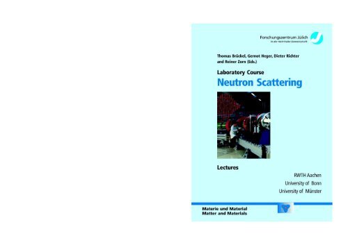
Thomas Brückel, Gernot Heger, Dieter Richter 

and Reiner Zorn (Eds .) 

Laboratory Course 

Neutron Scattering 

Lectures 

Materie und Material 

Matter and Materials 

Forschungszentrum Jülich 

in der Hefmhoftz-Gemeinschaft 

RWTH Aachen 

University of Bonn 

University of Münster

Schriften des Forschungszentrums Jülich 

Reihe Materie und Material / Matter and Materials Volume 15

Forschungszentrum Jülich GmbH 

Institut für Festkörperforschung 

Thomas Brückel, Gernot Heger, Dieter Richter 

and Reiner Zorn (Editors) 

Neutron Scattering 

Lectures of the Laboratory course 

held at the Forschungszentrum Jülich 

In cooperation with 

RWTH Aachen, University of Bonn and University of Münster 


Reihe Materie und Material / Matter and Materials Volume 15 

ISSN 1433-5506 ISBN 3-89336-324-6

Bibliographic information published by Die Deutsche Bibliothek 

Die Deutsche Bibliothek lists this publication in the Deutsche 

Nationalbibliografie; detailed bibliographic data is available in the 

Internet at . 

Publisher and Forschungszentrum Jülich GmbH 

Distributor : Central Library 

52425 Jülich 

Phone +49 (0) 24 61 61 53 68 . Fax +49 (0) 24 61 61 61 03 

e-mail : zb-publikation@fz-juelich .d e 

Internet : http ://wwvv.fz-juelich .de/zb 

Cover Design : Grafische Betriebe, Forschungszentrum Jülich GmbH 

Printer : Grafische Betriebe, Forschungszentrum Jülich GmbH 

Copyright : 

Forschungszentrum Jülich 2003 


Reihe Materie und Material / Matter and Materials, Volume 15 

New revised edition from Matter and Materials Volume 9 

ISSN 1433-5506 

ISBN 3-89336-324-6 

Neither this book nor any part may be reproduced or transmitted in any form or by any means, 

electronic or mechanical, including photocopying, microfilming, and recording, or by any 

information storage and retrieval system, without permission in writing from the publisher .

Contents 

1 Neutron Sources H . Conrad 

2 Properties of the Neutron, Elementary Scattering Processes D . Richter 

3 Elastic Scattering from Many-Body Systems Th . Brückel 

4 Polarization Analysis w . Schweika 

5 Correlation Functions Measured by Scattering Experiments R . Zorn 

6 Continuum Description : 

D . Richter 

Grazing Incidence Neutron Scattering O .H . Seeck 

7 Diffractometer G . Heger 

8 Small-angle Scattering and Reflectometry D . Schwahn 

9 Crystal Spectrometer : 

Triple-axis and Back-scattering Spectrometer F . Güthoff 

H . Grimm 

10 Time-of Flight Spectrometers M . Monkenbusch 

11 Neutron Spin-echo Spectrometer, NSE M . Monkenbusch 

R . Zorn 

12 Structure Determination G . Heger 

13 Inelastic Neutron Scattering : Phonons and Magnons M . Braden 

14 Soft Matter : Structure D . Schwahn 

15 Polymer Dynamics D . Richter 

16 Magnetism Th . Brückel 

17 Translation and Rotation M . Prager 

18 Texture in Materials and Earth Sciences w . Schäfer

Neutron Sources 

Harald Conrad

1 .1 Introductory remarks 

1 . Neutron Sources 

Harald Conrad 

Slow neutrons are a virtually unique probe for the investigation of structure and dynamics of 

condensed matter and biomolecules . Neutrons are called slow, if their kinetic energy is below 

1 keV. As the first neutrons used as microscopic probes were generated in nuclear reactors, 

historic terms like thermal neutrons are also frequently used in the classification of neutrons . 

In reactor physics the term thermal is used to distinguish these neutrons, which sustain the 

nuclear chain reaction, from the fart fission neutrons with energies of several MeV . Thermal 

neutrons, i.e . with an average kinetic energy of - 25 meV, are of particular interest in the 

context of this course . They are in thermal equilibrium with an adequate slowing down me- 

dium (moderator) like graphite, light or heavy water at ambient temperature (kBT - 25 meV) . 

With the availability of cryogenic moderators, cold neutrons ( = 3 meV) became important 

in recent decades, too . Strictly speaking, cold or so called trot neutrons ( = 200 meV) have 

to bc considered as thermal, too, because these are neutron gases in thermal equilibrium with 

a moderator at a particular temperature . Cold neutrons are in equilibrium with a cryogenic 

moderator, e .g . liquid hydrogen at 20 K or solid methane at liquid nitrogen temperature, 77 K . 

Hot neutrons are those in equilibrium with e .g . a graphite block heated to 2000 K, say . 

These trot neutrons and the even more energetic, so called epithermal neutrons (E > 1 eV) 

may in the future gain importance for scattering experiments, in particular with respect to 

pulsed accelerator driven neutron sources (sec below). But it is important to realize that there 

are no primary sources known, which directly deliver neutrons in the relevant energy range of 

typically 10 -3 eV < E < 1 eV . All existing sources emit primary neutrons with energies of 

about 10 6 eV or above and we are left with the difficult task to reduce the neutron energy 

between 6 and 9 orders of magnitude (moderation) . 

1 .2 Free Neutrons 

Free neutrons are unstable (half life about 12 minutes) . As a nuclear constituent they are sta- 

ble, though, and as bound particles virtually ubiquitous, except in light hydrogen. So, the only 

means of generating free neutrons are nuclear reactions . There is a variety of possible reac- 

tions, mostly forced ones, although spontaneous neutron emission is known to exist as well. A

number of neutron sources is described in the Appendix, in particular with respect to the 

achievable intensities . There are, of course, other criteria (e.g . cost or technical limitations), 

but for the neutron scattering experiment the highest possible signal (intensity) at the detec- 

tor is decisive . The quality of an experiment strongly depends on the counting statistics, 

which in turn govems the resolution capability of a neutron diffractometer or spectrometer . 

This criterion excludes most of the sources described in the Appendix for modem neutron 

scattering instruments, although electron accelerators for (y,n)-reactions were successfully 

utilized for a certain time . For other applications like medical or in nuclear and plasma 

physics those sources were and still are of importance . 

In the following we will explain in greater detail the two most important sources for neu- 

tron scattering experiments : the nuclear reactor and the spallation source . 

1 .3 The nuclear reactor as a neutron source 

Fission of a single 235U nucleus with one thermal neutron releases on average 2 .5 fast neu- 

trons with energies around 1 MeV . So, this is more than needed to sustain a chain reaction . 

Therefore we can withdraw typically 1 neutron per fission for puiposes like neutron scattering 

experiments without disturbing the chain reaction. The source strengths Q(n/s), i .e. neutrons 

emitted per second, achievable with these surplus neutrons are limited in particular by prob- 

lems ofremoving the energy released, which is about 200 MeV per fission. Using the relation 

1 eV = 1.6x10 -19 Ws we get Q - 3x10 16 n/s per MW reactor power to be removed . As men- 

tioned in the introduction the fast neutrons have to be slowed down to thermal energies to be 

useful for neutron scattering . 

The stochastic nature ofthe slowing down of neutrons by collisions with light nuclei ofthe 

moderator medium (e .g . protons in water) leads to the notion of a neutron flux ~D as a quality 

criterion for thermal neutron sources . This flux is defined as the number of (thermal) neutrons 

per second isotropically penetrating a unit area . In order to calculate the flux d)(r) for a given 

source distribution Q(r) (the fuel elements of a reactor core submersed in a moderator me- 

dium) we had to solve the general transport (Boltzmann) equation . But there are no analytical 

solutions possible for realistic geometries of reactor cores [1] . An estimate, however, will be 

given for simple model : a point source located in the center ofa spherical moderator vessel. If 

the radius of the vessel is equal to the so called slowing down length Ls [2], then 37% of the 

source neutrons become thermal . Using the deflnition (Dt, = v ,l, - n (average neutron velocity 

Pu,), where the stationaiy neutron density n is given by a balance equation, viz . n = q ' ti (bal- 

ance = production rate - life time) with q as the so called slowing down density, we have

d) f, = v a, , q - ti = P a, - 0 .37 Q / (47c Ls 3 /3) 'T, (1 .1) 

where the slowing down density q is the number of neutrons slowed down to thermal energies 

(i .e . to about 25 meV) per unit volume and per second. For a point source of strength Q in the 

center of a spherical moderator volume of radius r = L s we obtain what we have inserted for q 

in (2 .1) . The life time (also called relaxation time) is given by [2] ti = (Y-abs'vth + D'BZ)-1 

where Y- .,b, and D are the coefficients of absorption and diffusion of neutrons, respectively, 

and B2 = (Tc/L s )2 a geometrical factor, the "buckling", which is a measure for the spatial flux 

distribution . Inserting numerical values, Ls = 29 cm, Eabs = 3x 10 -5 cm- ' and D = 2x10 5 cm2/s 

for heavy water (Jülich's research reactor FRJ-2 is heavy water moderated), we obtain with 

the source strength Q - 3x10 16 n/(s MW) a thermal neutron flux fia, = 1 .1x 10 13 n/(cm2s MW) . 

Extrapolating this to 23 MW, the power of the FRJ-2, we obtain a)a, = 2.5x1014 n/(cm2 s) . This 

is only 25% too big, a suiprisingly good result taking into accourt the non realistic assumption 

Fie. 1 . 1 Horizontal cut through the reactor block of the Jülich research reactor FR7-2. 

(The numbers below the acronyms are the beam charnel heights above thefloor of the experimental 

hall.)

ofthe reactor being a point source . In fact the core of the FRJ-2 consists of 25 tubular, 60 cm 

high fuel elements arranged within a lateral grid of about one meter in diameter . The core is 

submersed in and cooled by heavy waten streaming through the tubes . Figure 1 .1 shows a plan 

cross sectional view ofthe reactor block . 

The FRJ-2 is operated with highly enriched uranium 235U . With the existing relaxed fuel 

element arrangement an essential neutron flux enhancement, e .g . by an order of magnitude, 

were only possible with a corresponding but unwanted power increase . A different possibility 

exists in compacting the core, a solution chosen for the high flux reactor at the Institut Laue- 

Langevin in Grenoble, France . In fact, its core consists of a single annular fuel element of 

40 cm outer and 20 cm inner diameter, respectively . Operated at 57 MW, a disturbed flux at 

the beam tube noses of fia, =1.2x10 15 n / (cm2 s) is obtained . 

Technical limitations 

We have just established a relation between neutron yield and reactor power released as heat . 

Disregarding for the moment investment and operation costs, the limiting factor for achiev- 

able neutron yields is the power or, to be more precise, the power density in the reactor core . 

This technically decisive factor, the power density (1VIW/liter), was not included in the 

number given in the previous section, because it depends on the details of the reactor, in 

particular the core size, the uranium enrichment and the fuel density in the fuel elements . The 

size of the primary neutron source (reactor core, target volume, etc.) is important for a high 

flux of thermal neutrons within the moderator . In Table 1 .A .1 of the Appendix a selection of 

reactions is given and related to its neutron yields and power densities . 

It is now well established that power densities in reactor cores cannot substantially be in- 

creased without unwanted and impracticable consequences, such as liquid sodium cooling . In 

particular, the service time of reactor vessel components like beam tube noses or cold sources 

would become intolerably short due to radiation damage . Experience with the Grenoble High 

Flux Reactor shows that these service times are of the order of seven years . Ten tunes higher 

fluxes would result in impracticable service times under one year . 

1 .4 Pulsed contra continuons sources 

Regarding these arguments, we may ask ourselves, whether high flux reactors have already 

reached a fondamental lirait . This were ce-tainly the case, if we expected a flux increase by 

another order of magnitude like the one observed in reactor development since the fifties (sec 

Table 1 .1).

Table 1 .1 Development ofthermalfuxes ofresearch reactors 

A flux increase by a factor of about 6 over that ofthe Grenoble reactor had been envisaged 

for a new research reactor in Oak Ridge, USA . This enhancement would have been only pos- 

sible by a power increase to 350 MW with a simultaneous increase of the average power den- 

sity by a factor of 4 compared to Grenoble . After ten years of planning, the US Department of 

Energy decided not to build this so called ANS (Advanced Neutron Source). 

At this point we have earnestly to ask, whether the decision was adequate to build ever 

more powerful but continuously operating reactors . From a technical point of view is was 

perhaps the easiest path, from the point of view of neutron scattering, on the other hand, it 

was by no means necessary or economic . In order to accept this we only have to realize that 

the two standard methods of neutron scattering, i .e. crystal and time of flight techniques, in 

any case only use a minute fraction (10-2 . . . 10-4 ) of the source flux. Monochromatization 

and/or chopping the primary beam as well as collimation and source to detector distance 

(shielding!) may even reduce the source flux by factors of 10-8 to 10-11 , depending on resolu- 

tion requirements . 

Period Example Flux (D [1013 

1950-60 FRM-1 München - 1 

1960-70 FRJ-2 Jülich -10 

1970-80 HFR Grenoble -100 

CM-2 S-1 ] 

1980-90 ? -1000 ??? 

Time of flight spectroscopy inefficiently utilizes the continuous reactor flux for two rea- 

sons, because it requires both a monochromatic and a pulsed beam . Crystal spectrometers and 

diffractometers use an extremely narrow energy band, too . The rest of the spectrum is literally 

wasted as heat . Obviously, time of flight techniques wich pulsed operation at the same average 

source power yield gain factors equal to the ratio of peak to average flux . With crystal tech- 

niques higher order Bragg reflections can be utilized, because they become distinguishable by 

their time of flight. In other words, the peak flux will be usable between pulses as well . 

So, without increasing the average power density, pulsed sources can deliver much higher 

peak fluxes, e.g. 50 times the HFR flux . Now, which type of pulsed source is to be preferred : 

a pulsed reactor or an accelerator driven source? This question is not easy to answer. Possibly 

it depends on the weights one is willing to assign to the particular arguments . Important ar- 

guments are cost, safety, pulse structure or the potential for other uses than neutron scattering .

If we set aside the costs and ask about safety, we can assert that accelerator driven sources 

(e .g . spallation sources) are inherently safc, because no critical configuration is needed for the 

neutron production . A pulsed reactor, on the other hand, bas to run periodically through a 

prompt super critical configuration . Therefore the external control mechanisms (absorbers) of 

the continuously operating reactor will not work. The power excursion must be limited by in- 

herent mechanisms, e .g . by the temperature rise of the fuel . Although it may be unlikely in re- 

ality, malfunctions of the necessarily mechanical insertion of excess reactivity (rotating parts 

of fuel or reflector) may lead to substantial damage of the reactor core . No problems exist in 

that respect with a spallation neutron source. Furthermore, the proton beam can be shut down 

within a few milliseconds . Neutron generation by protons enables the shaping of pulse struc- 

tures (pulse duration below 1 microsecond, arbitrary pulse repetition rates) basically unfeasi- 

ble with mechanical devices . 

1 .5 The Spallation Neutron Source 

1 .5 .1 The spallation reaction 

For kinetic energies above about 120 MeV, protons (or neutrons) cause a reaction in atomic 

nuclei, which leads to a release of a large number of neutrons, protons, mesons (if the proton 

energy is above 400 MeV), nuclear fragments and y-radiation . This kind of nuclear disinte- 

gration has been named spallation, because it resembles spalling ofa stone with a hammer . 

The spallation reaction is a two stage process, which can be distinguished by the spatial 

and spectral distribution of the emitted neutrons . This is depicted schematically in Figure 1 .2 . 

f -t 

f',',l' c', t 

Fig. 1.2 The spal1crlion process 

l1Et1a tiu I?~i t Yittcl 1lFt-l,i1 

P'ntsPtfy ~ ;Si1

In stage 1 the primary proton knocks on a nucleon, which in turn knocks on another nu- 

cleon of thé saine nucleus (intea-nuclear cascade) or of a différent nucleus (inter-nuclear cas- 

cade) . With increasing energy of thé primaiy particle thé nucléons kicked out of thé nuclei 

will for kinematic reasons (transformation from center of mass to laboratoiy system) be 

emitted into decreasing solid angles around forward direction . The energy distribution of thé 

cascade particles extends up to thé primary proton energy . Alter emission of thé cascade par- 

ticles thé nuclei are in a highly excited state, whose energy is released in stage 2 mainly by 

evaporation ofneutrons, protons, deuterons, a-particles and heavier fragments as well as y-ra- 

diation . Depending on thé particular evaporation reaction course, différent radioactive nuclei 

remain . These evaporation neutrons are isotropically emitted. They are thé primary source 

neutrons, in which we are interested in thé prescrit context . The spectrum of thé evaporation 

neutrons is very similar to that of nuclear fission and has a maximum at about 2 MeV . This is 

thé veiy reason, why we cari utilize thé spallation neutrons as with a fission reactor . 

The yield of evaporation neutrons increases with proton energy and depends on thé target 

material . The following expression for thé yield has been found empirically 

Y = f - (A + 20) - (E - b) neutrons / proton, (1 .2) 

where A is thé mass number of thé target material (9

For uranium, which releases neutrons by fission as well, b = 0 .02 GeV. In Figure 1 .3 the yield 

for lead and uranium is plotted and related to the energy released per neutron . The latter has 

important consequences as already discussed in section 1 .3 . 

1 .5 .2 Technical details 

A spallation neutron source consists of three important components, the accelerator, the target 

and the moderators . For reasons discussed in sections 1 .3 and 1 .4 the planned European 

Spallation Source (ESS) will be pulsed . 

1 .5.2.1 The accelerator 

The concept of the ESS envisages a pulsed linear accelerator (linac), which will supply the 

full beam power, and two subsequent storage rings for compressing the pulses from the linac . 

The ESS design parameters are : 

linac proton energy 1 .33 GeV, 

average curr ent 3 .75 mA 

average beam power 5 MW 

linac peak current 0 .1 A 

ring peak current 100 A 

repetition rate 50 S-1 

linac pulse duration 1 ms 

pulse duration after compression 1 ps 

300 m long (superconducting cavities) 

ring diameter : 52 m 

It is worthwhile to point out that we need a rather complex machine to accelerate particles 

from rest to kinetic energies of 1 GeV or above and extract them in pulses of only 1 ps dura- 

tion . For the case of the ESS we need five stages of acceleration and compression such as 

- electrostatic acceleration to 50 keV 

- radio frequency quadrupole (RFQ) acceleration from 50 keV to 5 MeV 

- drift tube linac (Alvarez-type) from 5 MeV to 70 MeV 

- superconducting multiple cavity linac from 70 MeV to 1330 MeV 

- two (!) compressor rings (space charge !) . 

1 .5.2.2 The target- solid or liquid? 

According to relation (1 .2), heavy elements (large mass number A) are favored as target can- 

didate materials, in particular the refractory metals tantalum, tungsten or rhenium, but also 

lead, bismuth or even uranium . Whatever material is selected, it will be subject to heavy mul- 

tiple loads . Firstly, about 60% of the 5 MW average beam power is dissipated within the tar-

get as heat, the rest is transported as released radiation to the target vicinity like moderators, 

reflector and shielding or is converted into nuclear binding energy . Secondly, all materials bit 

by protons (and fast neutrons) will suffer from radiation damage. Finally, the extremely short 

proton pulses generate shock-like pressure waves in target and structural materials, which 

may substantially reduce the target seivice life. In order to both keep average target tempera- 

turcs low and reduce specific radiation damage and loads due to dynamic effects from shock 

waves, a solid rotating target is conceivable and bas been proposed for the ESS . As any solid 

target has to be cooled, it will inevitably be "diluted" by the coolant, whereby the primary 

source's luminosity will be diminished . One should therefore operate the target in its liquid 

state avoiding an additional cooling medium. Radiation damage would be no longer a prob- 

lem wich the target, but of course with its container . Obviously, the refractoiy metals are ex- 

cluded due to their high melting points. So we are left with elements like lead, bismuth, the 

Pb-Bi eutectic or - of course - mercury . In tact, mercury has been chosen for the ESS, because 

it was also shown to exhibit favorable neutron yield conditions as presented in Figure 1 .4 . 

Fig. 1 .4 Calculated axial leakage distributions offast neutronsfrom a lead-nefected 

mercury target compared to waten cooled tantalum and tungsten targets, respectively . 

The dimensions of a target along the beam path will reasonably be chosen according to the 

range of the protons of given kinetic energy . For mercury and the ESS energy of 1 .33 GeV 

this is about 70 cm . Lateral target dimensions are optimized so that the moderators are not too 

far from the proton beam axis (solid angle!) . A typical target-moderator-reflector configura- 

tion is depicted schematically in Figure 1 .5 .

neutron beann channels 

Fi 1 .5 Schematic vertical and horizontal cuts through the innerpart ofthe target block. 

1 .5.2.3 The moderators 

We will now turn to the "heart" ofthe facility, the moderators, which were just shown in the 

last figure above in their relative positions next to the target . As the upper and lower faces of 

the target are equivalent for symmetry reasons with respect to the emission of fast neutrons, it 

is obvious to exploit both sides with moderators . The question now is, whether we shall use 

D 20 as the slowing down medium like in all modern medium and high flux reactors or possi- 

bly H2O? As we have discussed in section 1 .4, not the highest possible average neutron flux is 

the only reasonable demand, but rather the highest possible peak flux for a given (or re- 

quested) average flux . In that respect, H2O is the preferred material due to its bigger slowing 

1-10

down power and stronger absorption for thermal neutrons (sec below) . The reason for this 

seemingly paradoxical demand for stronger absorption is that the achievable neutron peak 

flux is not only proportional to the proton peak current, but also depends on the storage time T 

(sec below) of thermal neutrons in the moderator . We should point out here that the slowing 

down time for H2O and D 20 is small compared to the storage time T. The neutron peak flux is 

given by the following expression, which is the result of a convolution of a proton pulse of 

duration tp with an exponential decay of the neutron field within the moderator wich storage 

(decay) time T. 

_ - rep -tp / r 

1) th = ')th ' -(i - e ) 

tp 

where 4) th , ~th are peak and average flux, respectively, and t,, is the time between pulses . 

In the limit tp -> 0 expression (1 .3) reduces to 4 th = _~ th - trep / z, i .e . even a 8-shaped cur- 

rent pulse results in a finite neutron peak flux . We see as well that in this case the peak flux is 

inversely proportional to the moderator storage time . Also with finite cunrent pulses a short 

storage time is important for obtaining large peak fluxes . The storage time T of a thermal neu- 

tron is a measure of the escape probability from the moderator and is obviously determined by 

both the geometry ofthe moderator vessel and the absorption cross section of the moderator 

medium (sec section 1 .3) and can be written [2] : 

T = ( vtn ' Y-abs + 3 D n2 / L2 ) - 1 (1 .4) 

where v t1, is the average neutron velocity, E abs the macroscopic absorption cross section, D 

the diffusion constant for thermal neutrons and L is a typical moderator dimension . The ab- 

sorption cross section of H2O is about 700 times bigger than that of D20 . If it were only for 

this reason, an H20-moderator had to bc small (small L in (1 .4)), because we want of course 

utilize the neutrons that leak from the moderator. So, a short storage time must not entirely bc 

due to self-absorption . As, on the other hand, H2O possesses the langest known slowing down 

density (the number of neutrons, which become thermal per cm3 and s), an H20-moderator 

anyhow does not need to be big . In section 1 .3 we have already quoted that within a spherical 

moderator vessel with its radius equal to the slowing down length Ls (= 18 cm for H20), 37% 

of the fast neutrons emitted from a point source located in the center become thermal. In fact, 

an H20-moderator must not bc essentially larger, because within a sphere with r = 23 cm al- 

ready 80% ofthe neutrons are lost due to absorption .

For these reasons a pulsed spallation source will have small (V - 1 .5 liter) H20-moderators 

for thermal neutrons . The corresponding storage time of such H20-moderators bas been 

measured and is i = 150 ps [3], which is in good agreement with the estimate according to 

(1 .4) . Small size and absorption diminish in any case the tune average neutron yield . In order 

to improve this without deteriorating the peak fluxes, two tricks are used. Firstly, a moderator 

is enclosed by a so-called reflector (see Fig . 1 .5), a strongly scattering ("reflecting") but non 

moderating material, i .e . a heavy element with a large scattering cross section like lead . Sec- 

ondly, the leakage probability from the moderator interior, i .e . a region of higher flux due to 

geometrical buckling (Chapter 1 .3), is enhanced by holes or grooves pointing toward the neu- 

tron beam holes. Both measures give gain factors of 2 each, whereby the reflector gain is so to 

speak "for free", because the anyway necessary lead or iron shielding bas the saine effect. A 

reflector can be imagined to effect such that it scatters fast neutrons back, which penetrated 

the moderator without being or insufficiently slowed down . Similar considerations hold as 

well for cold moderators employed with spallation sources (Fig . 1 .5) . 

As a final remark let us point out that the overall appearance of a target station can hardly 

be told from a reactor hall with the respective experimental equipment in place . In both cases 

neutrons are extracted from the moderators by beam channels or guide tubes and transported 

to the various scattering instruments . 

In the following Table 1 .2 the expected and experimentally supported flux data of ESS are 

shown and compared te , those of existing sources . 

* with neutron chopper 100 s 1 

High flux reactor 

(HFR) 

Grenoble R 

Pulsed reactor 

HiR-H 

Dubna (R 

Tab . 1 .2 Comparison ofthe performance of varions modern neutron sources 

1-12 

Spallation source 

ISIS 

Chilton 

ESS 

Hg-Target 

H2O Moderator 

4 [cm -' s-' ] 10 15 2 - 1016 4 .5- 10 15 1 .4- 10 17 

(U[cm-2S-' 1 

Pulse repetition rate v [s-1 1 

10 15 2 . 1013 7 - 1012 0.6 . 

- 5 50 50 

Pulse duration [10-6 s] - 250 30 165 

dl0"cm -2 S -1 ] l* 1 2 .2 70 

()15

Appendix 

Neutron Sources - an overview [4] 

1 .A.1 Spontaneous nuclear reactions 

Although every heavy nucleus is unstable against spontaneous fission, this reaction is gener- 

ally suppressed by a-decays beforehand . With the advent of nuclear reactors, on the other 

hand, an exotic isotope, 252Cf, became available in suffcient amount from reprocessing spent 

nuclear fuel, where 3% of the decays are by spontaneous fission. The rest is a-decay . The 

data of a 252Cf-source are : 

- yield: 3 .75 neutrons / fission 

resp . 2.34 x 1012 neutrons / (gram s) 

- half life : 2 .65 y (including a-decay) 

- average neutron energy : 2.14 MeV (fission spectrum) 

1 .A.2 Forced nuclear reactions 

In this case we can distinguish between reactions initiated by both charged and neutral parti- 

cles . In this context y-quanta are regarded as neutral "particles". 

1 .A .2 .1 Reactions with charged particles 

Although we will restrict the discussion to light ions such as protons, deuterons and a-parti- 

cles, a wide field is covered from the historically important radium-beryllium-source to the 

latest sources like plasma focus or spallation sources . 

(a,n)-Reactions 

Reaction partners with these sources are either natural (Radium, Polonium) or artificial 

(Americium, Curium) radioactive isotopes and a light element such as Beryllium as target 

material . Using a radium-beryllium-source Bothe and Becker discovered in 1930 a new 

particle, which they failed to identify it as the neutron . Two years later Chadwick accom- 

plished this earning him the Nobel prize for this feat. Modern sources employ artificial iso- 

topes alloyed with Beryllium . Yields are between 10 -4 and 10-3 neutrons per particle . The 

technical parameters of a modern 241 Am/Be- source are : 

- yield: 0 .9 x 10 7 neutrons / s per gram 

- half life : 433 y 

- neutron energy : a few MeV (complex line spectrum) 

1- 1 3 

241

(p,n)- and (d n)-Reactions 

Bombarding targets (Be, . . . , U) with protons or deuterons ofmedium energy (Eki, < 50 MeV), 

either neutrons are released foira the target nuclei in the case of protons or the neutrons are 

stripped from the deuterons during the impact and thereby released. Yields are of the order of 

10-2 n/p resp . 10 14 n/s per milli-Ampere . 

An interesting special case is the reaction between the two heavy hydrogen isotopes, be- 

cause it can be exploited in two différent ways. One variant is thé so-called neutron genera- 

tor utilizing thé large reaction cross section of thé D-T-reaction, which peaks already at vely 

low deuteron energies (5 barn at 0 .1 MeV) . With this low particle energy thé emitted neutrons 

are virtually mono-energetic (E = 14 MeV) and thé émission is isotropie . The target may be 

gaseous or Tritium dissolved in adequate metals (Ti, Zr) . The yield for a D-T-neutron gen- 

erator with Ek; (d+) = 0 .1 MeV is of thé order of 10 11 neutrons/s per milli-Ampere . 

The second variant of exploiting thé D-T-reaction is thé plasma source . In this source both 

gases are completely ionized by applying high pressure and temperature forming a homoge- 

neous plasma, which releases neutrons via thé fusion reaction. In principle, this is thé same 

reaction as with thé neutron generator . Such sources operate in a pulsed mode, because thé 

plasma bas to be ignited by repeated compression . Due to thé need for this compression this 

spécial kind of a plasma source is also called thé plasma focus . Up to now yields of about 

3 x 10 12 neutrons / s have been obtained experimentally . Planned facilities are expected to de- 

liver 10 16 neutrons / s . 

Chapter 1 .5 bas already been dedicated in greater detail to (p,n)- or (d,n)-reactions at high 

particle energies (> 100 MeV), which lead to spalling of thé target nuclei ("spallation") . At 

this point we only want to give a typical number for thé neutron yield for comparison with thé 

other reactions quoted in this Appendix: 

- yield (for 1 GeV protons on lead) : 25 neutrons / proton 

resp . 1 .5 x 10 1 ' neutrons / s per milli-Ampere 

- average neutron energy : 3 MeV (evaporation spectrum) 

+ cascade neutrons (up to proton energy) . 

1.A .2.2 Reactions with neutral "particles" 

(yn)-Reactions (photonuclear reactions) 

Gamma radiation of radioactive isotopes can release so called photoneutrons, a process, 

which is indeed exploited in devices analogous to (a,n)-sources . A typically spherical y- 

source of a few centimeters in diameter is enclosed by a shell of target material . Due to the 

extremely high y-activities needed, even weakest neutron sources (106 n/s) can only be hand- 

1-14

led remotely. It is rauch more convenient to turn on the source when needed by replacing y- 

radiation by bremsstrahlung generated by electron bombardment of a heavy metal target . 

Using e.g . 35 MeV electrons, we obtain a yield of about 10 -2 n/e resp . 0.8 x 10 14 n/s per mA . 

Neutron induced nuclearfission (thé nuclear reacior) 

Of all neutron sources realized up to now, nuclear reactors are still thé most intense ones . 

We had therefore dedicated a detailed chapter for this kind of source (chapter 1.3) . 

For comparison we have compiled thé yields, heat deposition, source strengths and power 

densities ofthé varions reactions in thé following Table 1.A .1 . 

Reaction Yield Heat deposition Source strength Source power 

[MeV / n] [n/s] Density 

/ Liter 

Spontaneous fission 252Cf 

* At thé hot spot 3 .3 MW/L. For 2 x 10 18 source neutrons per second this gives a thermal flux of 10' 5 n cm2 s 

Table I.A.1 Yield, heat déposition, source strength andpower densityfor selected neutron 

sources 

Literature 

3 .75 n/fission 100 2 x 1012 9-1 0.9 

39 W/ 

9Be (d,n) (15 meV) 1 .2 x 10-2 n/d 1200 8 x 1013 mA-1 - 

3H (d,n) (0 .2 MeV) 8 x 10-5 n/d 2500 5 x 101 ' mA"' - 

Spallation 28 n/p 20 10 18 0.5 (ESS) 

1.33 GeV protons on Hg 

Photoproduction 1 .7 x 10 -2 n/e 2000 4 x 10 14 5 (Harwell) 

W e,n 35 MeV 

235U frssion 1 n/fission 200 2 x 1018 1 .2* 

nuclear chain reaction (HFRGrenoble 

[1] S. Glasstone, A. Sesonske, Nuclear Reactor Engineering ; van Nostrand Comp . Inc ., 1963 

[2] K.H . Beckurts, K.Wirtz, Neutron Physics ; Springer-Verlag, 1964 

[3] G. Bauer, H. Conrad, K. Friedrich, G. Milleret,H. Spitzer; Proceedings 5 11' International 

Con£ on Advanced Neutron Sources, Jül-Conf-45, ISSN 0344-5789, 1981 

[4] S. Cierjacks, Neutron Sources for Basic Physics and Applications ; Pergamon Press, 1983 

1- 1 5

Properties of the Neutron 

Elementary Scattering Processes 

Dieter Richter

2 . Properties of the neutron, elementarg 

scattering processes 

2 .1 A few remarks on history 

D. Richter 

In 1932 the neutron was discovered by Chadwick . The naine results from the observation that 

the neutron apparently does not possess an electric charge : it is neutral . Today, one knows 

that the neutron is an ensemble of one up quark and two down quarks . According to the 

standard theory, the total charge therefore amounts to 2/3 é + 2 ( -1/3 e) = 0 . At prescrit this 

theoretical statement is proven with a precision of- 10 -21 e-1 

Only four years later in 1936 Hahn and Meitner obselved the ferst man-made nuclear fission . 

In the saine year also the frst neutron scattering experiment was performed. Its set-up is 

shown in Fig .2 .1 . Neutrons were taken from a radium beryllium source which was covered by 

a paraffm moderator . From that moderator neutron beams were extracted such that they bit 

magnesium oxide single crystals which were mounted on a cylindrical circumference under 

the appropriate Bragg angle. After reflection they were guided to a detector which was 

mounted opposite to the radium-belyllium source . In order to avoid any directly penetrating 

neutrons a big piece of absorber was mounted in between the detector and the source . 

Magnesium ozidc singlc 

crystals mountcd around 

cylindrical circumfercncc 

Figure 2 .1 : Mitchell and Powers's apparatus for demonstrating the diffraction of neutrons 

(alter Mitchell and Powers 1936) .

In December 1942 Ferme build his ferst nuclear reactor in Chicago - the so called Chicago 

pile - which led to the frst controlled nuclear chain reaction . Only one year later the Oak 

Ridge Graphite Reactor went critical . It had a power of 3.5MW and was originally used for 

the production of fissionable material . Fig .2 .2 shows this reactor which by now is a national 

historic landmark . At this reactor, Shull build the ferst neutron diffractometer which became 

operationally at the end of 1945 . At that instrument the frst antiferromagnetic structure 

(Mn02) was solved (Shull, Noble Price 1994). At the end of the 40's and the beginneng of the 

50's nuclear reactors for neutron research came into operation in several countries . 1954 the 

Canadian NRU Reactor in Chalk River was the most powerful neutron source wich a flux of 

3-10 14n/cm 2s 1 . There Brockhouse developed the triple axis spectrometer which was 

designed, in order to observe inelastic neutron scattering and in particular to investigate 

elementary excitations in solids . For this achievement Brockhouse received the Nobel Price in 

1994 . Another milestone in neutron scattering was the installation of the ferst cold source in 

Harwell (Great Britain) . This cold source allowed to moderate neutrons to liquid hydrogen 

temperatures with the effect that for the ferst time long wavelength neutrons became available 

in large quantities . 

Figure 2 .2 : View ofthe Oak Ridge Graphite Reactor . 

2-2

In the 60's the ferst high flux reactor specially designed for beam hole experiments became 

critical in Brookhaven (USA) . It provided a flux of 10 15 n/cmZs1. For research reactors this 

level of flux was not significantly surpassed since then. Finally, 1972 the high flux reactor at 

the Institute Laue Langevin in Grenoble (France) went into operation . This reactor since then 

constitutes the most powerful neutron source worldwide . 

In parallel using proton accelerators already beginning in the 60's, another path for neutron 

production was developed . Pioneering work was performed at the Argonne National 

Laboratory (USA) . At present the most powerful Neutron Spallation Source is situated at the 

Rutherford Laboratoiy in Great Britain which bases on a proton beam of about 200KW beam 

power. The future of neutron scattering will most probably go along the lines of spallation 

sources . At present in the United States the construction of a 2.5MW spallation source has 

commenced wich the aim to get operational in 2005 . European plans to build a Megawatt 

Spallation Source are still under development and hopefully a European decision for the 

European Spallation Source (ESS) will be reached in the year 2003 . 

After the war, Germany was late in the development of neutron tools for research . Only in 

1955 international agreements allowed a peaceful use of nuclear research. In the saine year 

the frst German Research Reactor became critical in Garching . In the early 60's powerful 

research reactors were build like for example the FRJ-2 reactor in Jülich which provides a 

flux of 2. 10 14 n/cxri Zs ' . Instrumental developments became a domain of German neutron 

research. A number of important German contributions in this field are the backscattering 

spectrometer, the neutron small angle scattering, the instruments for diffuse neutron scattering 

and high resolution time of flight machines . 

2 .2 Properties of the neutron 

The neutron is a radioactive particle with a mass of m = 1.675 . 10 -27kg . It decays alter a 

mean lifetime of z= 889 .1 ± 1 .8s into a proton, an electron and an antineutrino (/3 decay) . 

n -> p+ + e + v (+ 0 .77 MeV) (2 .1) 

2-3

For any practical application the imite lifetime of the neutron has no consequence . At neutron 

velocities in the order of 1000m/s and distances in experiments up te, 100m lifetime effects 

are negligible . 

The neutron cames a spin of 1/2 which is accompanied by a magnetic dipole moment 

The neutron wavelengths is obtained from the de Broglie relation 

AM 

Ii" = -1 .913 p,, (2 .2) 

where uN is the nuclear magneton . The kinetic energy of the neutron E n = z ni, - un may be 

given in différent units as follows 

1 meV = 1 .602 - 10 -22 J =:> 8.066 cm- ' 

since E = hv 1 meV=> 0.2418 . 10 12 Hz 

since E = kBT : 1 meV=> 11 .60 K 

_ h h 

m n Un =/( 21n E" )1i2 

According to the conditions for moderation, neutrons in different wavelength regimes are 

separated into different categories as displayed in Fig .2 .3 . They are produced by moderation 

in particular moderators which are kept at different temperatures . 

hot thermal cold very cold ultra cold 

v v v 

10 -2 10-4 10 -6 

2-4 

102 

E [eV] 

Figure 2 .3 : Relation between neutron wavelength and their corresponding kinetic energies . 

(2 .3)

Hot neutrons in reactors are obtained from hot sources at temperatures around 2000K . 

Thermal neutrons evolve from ambient moderators while cold neutrons are obtained from 

mainly liquid hydrogen or deuterium moderators . The velocity distribution of the neutrons 

evolving from such a moderator are given by a Maxwell velocity distribution 

o (u ) = vs exp 

Thereby, 0(u) du is the number of neutrons which are emitted through an unit area per 

second with velocities between v and v+dv. Fig .2 .4 displays Maxwellian flux distributions 

for the three types of moderators discussed above . 

ulkm s - ' 

2 .1 compares the most important properties ofboth radiations . 

2-5 

(2 .4) 

Figure 2 .4 : Velocity distributions of neutrons from cold (25K), thermal (300K) and hot 

(2000K) moderators . 

Finally, Neutrons as well as X-rays are used for scattering experiments on materials . Table

2 .3 Neutron production 

Table 2 .1 : 

Comparison of X-rays and neutrons 

Neutrons are generated by nuclear reactions . For the investigation ofmatter a large luminosity 

that means a high flux of neutrons 0 ofthe requested energy range is essential . Such fluxes at 

prescrit cari only be obtained through nuclear fission or spallation . Both are schematically 

displayed in Fig .2 .5 . 

In nuclear fission a thermal neutron is absorbed by an 235U nucleus . The thereby highly 

excited nucleus fissions into a number of smaller nuclei of middle heavy elements and in 

addition into 2-5 (on average 2 .5) highly energetic fast fission neutrons . Typical energies are 

in the rage of several MeV. In order to undertain a nuclear chain reaction, on the average 1 .5 

moderated neutrons are necessaiy . At a balance a research reactor delivers about 1 neutron per 

fission event . 

X-rays are transversal 

electromagnetic waves 

The most powerful research reactor worldwide, the IIFR at the Institute Laue Langevin in 

Grenoble, produces a neutron flux of

elated values for the FRJ-2 reactor in Jülich for comparison are (ah,, = 2 - 10 14 n/cm2s at 23 

MW . 

th ~f rI°i~f r 

fL~lll[ 3fl 

f.=l ,;.f 

sion 

cI f e. 

'21'.ctP_: 

rlr.4t tttfa ui 1Y4r 

i 

1ii :td, -< 1- 

ius.f -t r s 

ip 

Figure 2 .5 : Schematic presentation of the fission and spallation process . 

In the spallation process highly energetic protons which are typically at energies of about 

1GeV hit a target of heavy nuclei like tungsten or tantalum . The proton excites the heavy 

nucleus strongly and in the event in the order of 20-25 neutrons are evaporated from such a 

nucleus . The energies of the spallation neutrons are typically in a range from several MeV up 

to hundreds of MeV. Other than a research reactor, a spallation neutron source can easily be 

operated in a pulsed mode, where a pulsed proton beam hits a target . At the spallation source 

ISIS at the Rutherford Laboratory for example, the repetition frequency amounts to 50Hz . In 

2-7 

1,

this way even at a comparatively low average neutron flux very high pulsed fluxes may be 

obtained . In the thermal range for example, the Rutherford source is able to surpass the ILL 

with respect to the peak flux significantly . Such pulsed sources can be used in particularly 

well for time of flight experiments which will be discussed later in the school . 

2 .4 Neutron detection 

Generally the detection of neutrons is performed indirectly through particular nuelear 

reactions which produce charged particles . A number of possible reactions are listed in 

Table 2 .2 . 

Proportionality counters operate wich a gas volume of 3He or BF 3 (enriched with' °B) . Such 

counters deliver sensitivities to nearly 100% . Scintillation counters absorb neutrons within a 

polymer or glass layer which is enriched by 6 Li and ZnS . Neutron absorption then leads to 

fluorescence radiation which is registered via a photo multiplayer or directly wich a 

photographie film. Finally, fission chambers use the n + 235U reaction and have generally only 

a low counting probability . They are mainly used in order to control the beam stability and are 

applied as monitors. 

Table 2 .2 : 

Nuclear reactions used for neutron detection . 

The cross sections are given in barns (lb =10 -28 m 2 ). 

Reaction Cross Section for Particles Energy Total Energy 

25meV neutrons generated [MeV] [MeV] 

P 0.57 0 .77 

n + 3He 5333 b 3 T 0 .2 

6 

n + Li 941 b 

3T 2 .74 4 .79 

4He 2 .05 

4He 1.47 2 .30 

n +' °B 3838 b 7 Li 0 .83 

n + 235U 

y 0.48(93%) 

681 b fission 1-2 

2-8

2 .5 Scattering amplitude and cross section, the Born approximation 

We now consider the scattering event by a fixed nucleus . The geometry for such a scattering 

process is sketched in Fig .2 .6 . The incoming neutrons are described by plane waves e'krr 

travelling in z -direction . At the target this plane wave interacts with a nucleus and is scattered 

into a solid angle S2 df. 

e ikr 

Incident 

neutrons 

r = (0, 0, Z) 

Figure 2.6 : Scattering geometiy for an incident plane wave scattered at a target . 

The partial cross section is defmed by 

_d6 _ current of scattered neutrons into (52, dÇ2) 

A2 current of incident neutrons 

Quantum mechanically the current is given by 

2mi (Y/*V y/-VvV/ *) 

For an incident plane wave yr= ezkr Eq.[2 .6] leads immediately to j = h~ , where V is 

n 

the normalization volume . The scattered spherical wave has the form 1 f(Ç2)e"" therej(~ 

r 

2-9 

(2 .5) 

(2 .6)

describes the solid angle dependent scattering amplitude. Inserting this form for the scattered 

wave into Eq .[2 .6] for large r 

J, _ hk If( ~2 )Iz dS2 2 .7) 

mn 

is obtained. Finally, inserting the incoming and scattered cunents into Eq .[2 .5] we obtain for 

the cross section 

d6 - I hk'I ml If (Ç2)12 dÇ2 - I f (sa)~z 

dS2 Ihklml dn 

du is also called differential cross section . We realize, that a scattering experiment delivers 

information on the absolute value of the scattering amplitude, but not on f(n) itself. 

Informations on the phases are lost. The total cross section is obtained by an integration over 

the solid angle 

(T = f d2 

du M 

12 

Our next task is the derivation off(n) in the so called Bom approximation . We start with the 

Schrödinger equation ofthe scattering problem 

z 

- -4+V(r) 

2m 

2- 10 

yr = EV/ 

(2 .8) 

(2 .9) 

(2 .10) 

where V(r) is the scattering potential . We note, that for scattering on a free nucleus the mass 

term in the kinetic energy has to be replaced by the reduced mass li = M mn . For large 

mn +M 

distances (r -> oo), V= 0 and we have E = h2k2l2m,, . Inserting into Eq.[2 .10] leads to the wave 

equation

(A+k2 ) yr = u(Z:) yr 

V( u~r)= z " r) 

The wave equation is solved by the appropriate Greenfunction 

(A2+k2)GL-r') = -4zd(r-r') (2 .12a) 

'b ~ -=' I 

G(r-L' ) = e 

Ir _ 0 

(2.12b) 

u (r) yr (r) = f dr' S (r - r') u(r') yr(r') (2 .12c) 

where G(r) is the Greenfunction solving the wave equation with the o-function as 

inhomogeneity . Using Eq.[2 .12c] the wave Eq.[2 .11] may be formally solved by 

v/ (r) = e'= _ 1 f dr' G (L-r') u ( L' ) V ( r' ) (2 .13) 

4; - 

In Eq .[2 .13] the first part is the solution of the homogenous equation and the second part the 

particular solution of the inhomogeneous one . The integral Eq .[2 .13] may now be solved by 

iteration. Starting with the incoming wave vP= eikr as the zero order solution, the v+ 1 order 

is obtained from the order vby 

e'k - 41 f G(r-L') u(L') y/v(r') d 3 r' (2 .14) 

In the Born approximation we consider the first order solution which describes single 

scattering processes . All higher order processes are then qualified as multiple scattering 

events . The Born approximation is valid for weak potentials . 6'°` 0 1 where a is the size 

a z 

of the scattering object . For a single nucleus this estimation gives about 10-7 and the Born 

approximation is well fulfilled . 

2- 1 1

We note one important exception, the dynamical scattering theory, which considers the 

scattering problem close to a Bragg reflection in a crystal . Then multiple beam interferences 

are important and the Born approximation ceases to apply . For most practical puiposes, 

however, the Born approximation is valid. Under the Born assumption the scattered wave 

function becomes 

y/ 

= er-r 

1 e`k~= 'I 2m, 

- - = V (I:') e 'kI dzr' (2 .15) 

4z Ir-r~I 

z 

In order to arrive at a final expression, we have to expand all expressions containing r and r' 

around r. Thereby, we consider that r' is a sample coordinate and small compared to r. We 

have 

Ir-r'I 

-r-r'- grad (r) = r-r' 

Inserting Eq.[2.16] into Eq.[2 .15] gives 

9 

ed'r' V/ e' - - - 

'- =` V (r') e'~I 

(2 .17) 

4z r hz 

Eq . [2 .17] may be written as 

1 ' - 1 + O 

Ir-r I r ( rr ) 

1 e'~ - =k=~' 2m 

k 

: direction ofthe scattered wave k' 

Irl 

EI 

(k'- IVI k) 

leads to the final expression for the cross section Eq .[2 .8] 

2- 12 

fp) 

1 

(2 .16) 

m 

e (2 .18) 

2Z hz 

r

We now also allow for inelastic processes, where the sample undergoes a change of its state 

from I Â) -> I Â') . For the cross section we now also have to consider the changes of state as 

well as different length of the wave vectors of the incoming and outgoing waves, which lead 

to factors k' and k in the cuvent calculation. 

d6 k' ~ m 

n 

(2 

dÇ2) (,k=, ;~) - k 2z 

2 

I(k',Z' IVI k,)1 2 

.20) 

The scattering event must fulfill energy and momentum conservation . With that we arrive 

fmally at the double differential cross section 

a26 

_ _k' M)n 

\ 2 

M aü) k (2z 

h2 

_du _ mn 

A2-~2z r2~ 

\2 

I(k' 

IVI 

k)I2 (2 .19) 

Pa 1 (k', a' IVI k,a)2 s(hw + (2 .21) 

The summation over Â is carried out over all possible initial states À of the system with their 

appropriate probability P Â. The sum over V is the surr over all final states, the o-function 

takes care of the energy conservation, thereby hao is the energy transfer of the neutron to the 

system . This double differential cross section will be discussed in detail in the lecture on 

correlation functions . 

2 .6 Elementary scattering processes 

2 .6 .1 The Fermi pseudo potential 

The interaction of the neutron with a nucleon occurs under the strong interaction on a length 

scale of 1 .5 - 10-15m. For that process, the Born criterium is not fulfilled and for the scattering 

process on a single nucleus the Born series would have to be summed up . Fortunately, this is 

a problem of nuclear physics and for the pulposes of neutron scattering a phenomenological 

approach suffices . Considering that the wavelengths of thermal neutrons are in the order of 

10-1°m we realize, that they are much larger than the dimension of a nucleus of about 10-15m. 

2- 13

Therefore, for any scattering event we may perform a separation into partial waves and 

consider only thé isotropie S-wave scattering . These scattering processes may bc described by 

one parameter thé scattering length b = bi + i - b2. Thereby bl describes scattering, while b2 is 

thé absorption part. For thermal neutrons thé scattering potential of a single nucleus becomes 

(Ferrai pseudo potential) 

= 2z b 

z 

V (r) 

Mn 

bS (L-R) (2 .22) 

The scattering lengths b have been measured as a fonction of neutron energy . For thermal and 

lower energies thé réal parts of these scattering lengths are constant and depend in an non- 

systematic way on thé number ofnucléons (sec Fig .2 .7). 

We realize, that there are positive as well as negative scattering lengths . Following a 

convention most of thé scattering lengths are positive . In this case, we have potential 

scattering with a phase shift of 180° between thé incoming and scattered wave . Negative 

values result from résonance scattering where thé neutrons penetrate thé nuclei and create a 

compound nucleus . The emitted neutrons do not undergo a phase shift. We also realize strong 

différences in thé scattering lengths for some isotopes . In particular important is thé différence 

in scattering length between hydrogen and deuterium (by, = -0 .374, bd =+0.667) . This 

significant différence in scattering length is thé basis of all contrast variation experiments in 

sort condensed matter research as well as in biology (sec later lectures) . We also note, that thé 

scattering lengths may dépend on thé relative orientation of thé neutron spin with respect to 

thé spin of thé scattering nucleus . Again a veiy prominent example is thé hydrogen. There thé 

scattering length for thé triplet state, neutron and hydrogen spins are parallel, amounts to 

bl,ipiet = 1 .04 - 10 -12cm while thé scattering length for thé singlet situation, neutron and 

hydrogen spins are antiparallel, is b,ingret = -0.474 - 10-12cm .

E 

ô 

ô 

x 

z 

w 

0 

z 

_w 

U 

N 

Figure 2 .7 : Scattering length of nuclei for thermal neutrons as a function of atomic weight . 

2 .6 .2 Coherent and incoherent scattering 

The scattering of neutrons depends on the isotope as well as on the relative spin orientations . 

We now will look into the consequences in regarding the elastic scattering from an ensemble 

of isotopes with the coordinates and scattering lengths {R, , b, } . The pseudo potential of this 

ensemble has the form 

V (L) - 2z b z 

Y, - R ) 

b, 8(r 

ni, l 

with Eq . [2 .l8] we may calculate the matrix element of Vbetween k and k' as 

~k' IVI = 2z b z 

k) 

m 

2zb 2 

m 

b f e>k'r ä (r _ R, ) e>~ d3 r 

2- 15 

b, eiQnr 

Q - k_ k' 

(2 .23) 

(2 .24) 

The matrix element is just a Fourier surr over the atomic positions decorated with the 

appropriate scattering length bi. The scattering cross section is obtained following Eq .[2.19] .

Thereby we now also consider the spin states ofthe nuclei before and after scattering s and s' . 

The initial state probabilities are given by Ps . 

d6_ - 

P exp (iQ (R -R,, » (s' b;, b s > (2 .25) 

dÇ2 SS' il' 

N 

We commence with spin independent interactions and assume that spatial coordinates and 

scattering lengths are not correlated - that means different isotopes are distributed randomly . 

Then Eq .[2 .25] may be evaluated to 

_d6 

M , 

(bâ b,) exp (iQ (R, -2R, .» 

In order to evaluate Eq.[2 .26] further, we introduce two scattering lengths averages - the 

mean square average and the mean scattering length . They are given by 

b2=1 ~b2 ; b =l ~,br 

N , 

With these defmitions, the average product of b, and bt' becomes 

(br br~ = (1 _ Srr, ) b2 +611 , b 2 

Finally, introducing Eq .[2 .28] into the expression for the cross section Eq.[2 .26] we obtain 

d6 -1 [(1 _ Srr') -2 + srr , -2] exp iQ ( Rj - Rj' ) 

dÇ2 i,, 

-2 

-)+ b2 b2 2.iQ~Ë exp, -R I ,) 

2- 16 

il , 

(2 .26) 

(2 .27) 

(2 .28) 

(2 .29) 

Obviously, the cross section contains two contributions . A coherent one where we have 

constructive interference of the neutron waves eminating from the different nuclei . This

scattering is observed with the average scattering length b . In addition there exists ineoherent 

scattering as a result ofthe isotope disorder . It is not able of interference and isotropie . 

We now consider spin dependent scattering from one isotope with the nuclear spinj. Both the 

nuclear spin as well as the neutron spin are statistically distributed. There exist two compound 

spin states : 

(i) neutron and nuclear spin are parallel : then I=j + 1/z. This spin state has the multiplicity 

of 2j + 2 . Its scattering length is b+ . 

(ii) neutron and nuclear spin are antiparallel I = j - 1/2 the multiplicity is 2j and the 

corresponding scattering length equals b - . The a priory probabilities for the compound 

spin states are given by the number of possibilities for their realization divided by the 

total number. 

+_ 2j+2 _ j+1 

p 

2j + 2 + 2j 2j + 1 

p - = j 

2j+1 

The corresponding average scattering lengths become 

(2 .30) 

b = p + b+ + p- b- (2 .31) 

b2 = p + b +2 + p - b -2 

We now consider the proton as an example . Here j= 1/2, b + =1 .04 . 10 -12 cm, 

b- = -4 .74 - 10-12cm, p+= 1/4, p = 1/4. Inserting into Eq .[2 .31] we fmd b = -0 .375 - 10-12 cm 

and b 2 = 6 .49 . 10-24cm2 . These values lead to a coherent cross section 

'7,.h = 4z . b 2 =1 .77 .10-24cm2 . For the incoherent cross section, we obtain 

6;,, = 4z - (b 2 - b2 ) = 79 .8 .10 -24 cm 2 . This value is the largest incoherent cross sections of all 

isotopes and makes the hydrogen atom the prime incoherent scatterer which can be exploited 

for hydrogen containing materials . 

2- 17

2 .7 Comparison between X-ray and neutron scattering 

Other than neutrons, X-rays are scattered by the electrons, which are distributed in space 

around the respective nucleus . This spatial distribution leads to an atomic form factor which is 

the Fourier transformed ofthe electron density distribution pi(! :). It depends in principle on the 

degree of ionisation of a nucleus but not on the isotope . 

Since the atomic radii (about 10 4 times larger than the radius of a nucleus) are comparable 

with the wavelength, the scattering amplitude f(Q) depends strongly on Q . Thus, with 

increasing scattering angle the scattering intensity drops significantly . Furthermore, the atom 

formfactor depends on the number of electrons Z and is given by 

Thereby, Z is the number of electrons of an atom or of an ion . Fig .2 .8 displays schematically 

sin B 

the atomic formfactor normalized to one as a function of 

t 

fi (Q) = f pi (r) exp (iQr) dV (2 .32) 

f; (Q=o)=Z 

sin 9 

(2 .33) 

Figure 2.8 : Schematic representation of normalized X-ray and magnetic neutron scattering 

form factors as a function of sin BQ. 

2- 18

For a spherical electron distribution pj(r), f(r) depend only on the absolute value of Q. For 

neutral atoms and possible ionic states they bas been calculated by Hartree-Fock calculations 

and may be found tabulated . 

Since the atomic form factors depend on the atomic number, the scattering contributions of 

light atoms for X-rays are only weak . Therefore, in structure determinations the precision of 

the localization of such important atoms like hydrogen, carbon or oxygen is limited in the 

presence of heavy atoms . Neutrons do not suffer from this problem since the scattering length 

for all atoms are about equal . 

In particular important is the case of hydrogen . In the bound state the density distribution of 

the only electron is typically shifted with respect to the proton position and an X-ray structure 

analysis in principle cannot give the precise hydrogen positions . On the other hand, bonding 

effects which are important for the understanding of the chemistry, may be precisely studied 

by X-ray electron density distributions . 

Atoms or ions with slightly different atom number like neighbouring elements in the periodic 

table are difficult to distinguish in X-ray experiments. Again, neutron scattering experiments 

also by the use ofthe proper isotope allow a by far better contrast creation . Such effects are in 

particular important for e .g . the 3d-elements . 

The paramagnetic moment of an atom or ion fcj results form the unpaired electrons . The 

density distribution of these electrons oj,n (r) is also named magnetization density or spin 

density and is a partial electron density compared to the total electron density pj(r) . Because 

of the magnetic dipole interaction, the amplitude of the magnetic neutron scattering is given 

in analogy to Eq.[2 .32] as the Fourier transformed of the magnetization density pjM (r) . The 

normalized scattering amplitude 

(Q) 1 fjM 

rI (r) -- exp pjM 

J 

2- 19 

(iQr dV 

(2 .34)

is also named magnetic form factor . If the spin density distribution is delocalised as e .g . for 

3d-elements, the magnetic form factor decays even more strongly than the X-ray analogue . 

2 .8 Conclusion : Why are neutrons interesting? 

Modem materials research together with the traditional scientifc interest in the understanding 

of condensed matter at the atomic scale requires a complete knowledge of the arrangement 

and the dynamcs of the atours or molecules and of their magnetic properties as well. This 

information can be obtained by investigating the interaction of the material in question with 

varies kinds of radiation such as visible light, X-rays or synchrotron radiation, electrons, ions 

and neutrons . Among them, neutrons play a unique role due to the inherent properties 

discussed above 

" their dynamic dipole moment allows the investigations of the magnetic properties of 

materials . 

" their large mass leads to a simultaneous sensitivity to the spatial and temporal scales that 

are characteristic of atomic distances and motions . 

" neutrons interact differently with different isotopes of the saure atomic species . This 

allows the experimentator to paint selected atoms or molecules by isotopes replacement. 

" neutrons can easily penetrate a thick material - an important advantage for material 

testing . 

" the interaction of the neutron with a nucleus bas a simple form (Born approximation) 

which facilitates the direct unambiguous theoretical interpretation of experimental data .

A more thorough introduction to neutron scattering may be found in the following 

books : 

[1] Bacon G.E ., Neutron Diffraction, Clarendon Press, Oxford (1975) 

[2] Bacon G.E. (Ed .), Fifty Years of Neutron Domaction : The advent of Neutron 

Scattering, Adam Hilger, Bristol (1986) 

Bée M., Quasielastic Neutron Scattering: Principles and Applications in Solid State 

Chemistry, Biology and Materials Science, Adam Hilger, Bristol (1988) 

[4] Lovesey S .W. and Springer T. (Eds.), Dynamics of Solids and Liquids by Neutron 

Scattering, Topics in Current Physics, Vol. 3, Springer Verlag, Berlin (1977) 

Lovesey S.W ., Theory ofNeutron Scatteringfrom Condensed Matter, Vol. 1 : Nuclear 

Scattering, Vol . 2 : Polarization Effects and Magnetic Scattering, Clarendon Press, 

Oxford (1984) 

[6] Sköld K . and Price D .L . (Eds .), Methods ofExperimental Physics, Vol. 23, Part A, B, 

C : Neutron Scattering, Academic Press, New York (1986) 

Springer T ., Quasielastic Neutron Scatteringfor the Investigation of Diffusive Motions 

in Solids and Liquids, Springer Tracts in Modern Physics, Vol . 64, Springer Verlag, 

Berlin (1972) 

[8] Squires G .L ., Introduction to the Theory of Thermal Neutron Scattering, Cambridge 

University Press, Cambridge (1978) 

[9] Williams W.G., Polarized Neutrons, Clarendon Press, Oxford (1988) 

[10] Willis B .T . (Ed.), Chemical Application of Thermal Neutron Scattering, Oxford 

University Press, Oxford (1973) 

[1l] Windsor C.G ., PulsedNeutron Scattering, Taylor & Francis, London (1981)

Elastic Scattering from Many-Body Systems 

Thomas Brückel

3 .1 Introduction 

3 . Elastie Seattering from Many-Body Systems 

Thomas Brückel, IFF, FZ-Jülich 

So far we have learnt about the production of neutrons and their interaction with a single 

atom. In this chapter, we will discuss the scattering of thermal neutrons from a sample 

containing many atoms . In the first part, we will assume that the atours are non-magnetic and 

only the scattering from the nucleus will be considered . In the second part, we will discuss the 

scattering from the spin- and orbital- angular momentum ofthe electrons in a magnetic solid . 

For simplification, we will assume in this chapter that the atours are rigidly fieed on 

equilibrium positions, i . e . they are not able to absorb recoil energy. This assumption is 

certainly no longer valid, if the neutrons are scattered from a gas, especially in the case of 

hydrogen, where neutron and the atour have nearly the saine mass . In this case, the neutron 

will change its velocity, respectively its energy, during the scattering event. This is just the 

process of moderation and without this so-called inelastic scattering (i. e . scattering connected 

wich a change of kinetic energy of the neutron) we would not have thermal neutrons at all . 

Also when scattered from a solid (glass, polycrystalline or single crystalline material) 

neutrons can change their velocity for example by creating sound waves (phonons) . However, 

in the case of scattering from a solid, there are always processes in which the recoil energy is 

being transfen ed to the Sample as a whole, so that the neutron energy change is negligible and 

the scattering process appears to be elastic . In this chapter we will restrict ourselves to only 

these scattering processes, during which the energy of the neutron is not changed. In 

subsequent chapters, we will leam how large the fraction of these elastic scattering processes 

is, as compared to all scattering processes . 

Quantum mechanics tells us that the representation of a neutron by a particle wave field 

enables us to describe interference effects during scattering . A sketch of the scattering process 

in the so-called Fraunhofer approximation is given in figure 3 .1 .

Fit. 3 .1 : A sketch of the scattering process in the Fraunhofer approximation, in which it is 

assumed that plane waves are incident on sample and detector due ta the fact that 

the distance source-sample and sample-detector, respectively, is signicantly 

larger than the site ofthe sample. 

In the Fraunhofer approximation it is assumed that the size of the sample is much smaller than 

the distance between sample and source and the distance between sample and detector, 

respectively . This assumption holds in most cases for neutron scattering experiments . Then 

the wave field incident on the sample can bc described as plane waves . We will further 

assume that the source emits neutrons of one given energy . In a real experiment, a so-called 

monochromator will select a certain energy from the white reactor spectrum. Altogether, this 

means that the incident wave can be completely described by a wave vector k . The saine holds 

for the wave incident on the detector, which can be described by a vector k' . In the case of 

elastic scattering (diffraction), we have : 

k=lkl =lk'I =k'=~ (3 .1) 

Let us define a so-called scattering vector by : 

Q=k-k' 

The magnitude of the scattering vector can be calculated from wave length k and scattering 

angle 26 as follows : 

3-2 

(3 .2)

Q = Q = k2 + k2 - 2kk' cos2B 

During a scattering experiment, the intensity distribution is being determined as a function of 

the scattering vector : 

I M (Q-) 

The proportionality factors arise from thé detailed geometiy ofthé experiment . Our task is to 

détermine thé arrangement of thé atoms in thé sample from thé knowledge of thé scattering 

cross section da/dÇ2(Q) . The relationship between scattered intensity and thé structure of thé 

sample is especially simple in thé approximation ofthé so-called kinematic scattering. In this 

case, multiple scattering events and thé extinction ofthé primary beam due to scattering in thé 

sample are being neglected . Following figure 3 .2, thé phase différence between a wave 

scattered at thé origin ofthé co-ordinate system and at thé position r is given by : 

k .r-k '.r=Q .r 

Fit. 3 .2 : A sketch illustrating thé phase différence between a beam being scattered at thé 

origin ofthé co-ordinate system and a beam scattered at thé position r. 

The scattered amplitude at thé position r is proportional to thé scatteringpower density ps (r) . 

The meaning of p, in thé case of neutron scattering will bc given later . The total scattered 

amplitude is given by a coherent superposition of thé scattering from all positions r within thé 

sample, i . e . by thé integral : 

3-3 

(3 .3) 

(3 .4) 

(3 .5)

A = 1Ps (r) - e'Q 'Yd3r (3 .6) 

Le. the scattered amplitude is connected with the scattering power density p s(r) by a simple 

Fourier transform: 

A = F( Ps ( ?") (3 .7) 

A knowledge of thé scattering amplitude for all scattering vectors Q allows us to determine 

via a Fourier transform thé scattering power density uniquely . This is thé complete 

information on thé sample, which can bc obtained by thé scattering experiment . 

Unfortunately, life is not so simple . There is thé more technical problem that one is unable to 

détermine thé scattering cross section for all values of (Q . The more fundamental problem, 

however, is given thé fact that normally thé amplitude of thé scattered wave is not 

measurable . Instead only the scattered intensity I - JA12 can bc determined . Therefore, the 

phase information is lost and thé simple reconstruction of thé scattering power density via a 

Fourier transform is no longer possible . This is thé so-called phaseprobleni of scattering . 

The question what we can learn about the structure of the sample from a scattering experiment 

despite this problem will bc the subject of the following chapters . For the moment, we will 

ask ourselves the question, which wavelength we have to choose to achieve atomic resolution. 

The distance between neighbouring atoms is in the order of a few times 0 .1 nm. In the 

following we will use the "natural atomic length unit" 1 A = 0 .1 nm . To obtain information on 

this length scale, a phase différence of about Q - a ~ 2 x has to be achieved, compare (3 .5) . 

According to (3 .3) Q~~ for typical scattering angles (2 0 ~ 60°) . Combining these two 

estimations, we end up with thé requirement that thé wavelength ;, has to be in thé order of 

thé inter-atomic distances, i . e . in thé order of 1 Â to achieve atomic resolution in a scattering 

experiment . This condition is ideally fulfilled for thermal neutrons . 

3-4

3 .2 Fundamental Scattering Theory 

In this chapter, we will give a simple formulation of scattering theory . Our purpose is to 

derive (3 .7) from fundamental principles . The conditions under which (3 .7) holds and the 

limitations of kinematical scattering theory will thus become clearer . During a fast reading 

this section can be skipped. More details can be found in [1] . 

In quantum mechanics, neutrons are described as particle wave fields through the Schrödinger 

equation : 

yr is the probability density amplitude, V the interaction potential . In the case ofpurely elastic 

E 1 

scattering E = E', the time dependence can be described by the factor exp~- iht ) . Assuming 

this time dependence, a wave equation for the spatial part ofthe probability density amplitude 

yr can be derived from (3 .8) : 

0`P +k2 (r)`Y = 0 (3 .9) 

In (3 .9) we have introduced a spatially vaiying wave vector with the magnitude square: 

k2 L) _ 2 (E - V~~~ (3 .10) 

Solutions of (3 .8) in empty space can be guessed immediately. They are given by plane waves 

IP = T0 expCiCk !: -~ with k2 = 

tJJ 2 

E . 2n The relations between magnitude of the wave 

vector, wave length and energy ofthe neutron E can be written in practical units : 

3-5 

(3 .8)

k[Ä-1 ]z 0.695 

E meV 

,,[Ä] 9.0451 VE meV (3 .11) 

E[meV ~t 81.8/2[Ä] 

To give an exaniple, neutrons of wavelength a, = 2.4 A have an energy of 14 .2 meV with a 

magnitude ofthe neutron wave vector ofk = 2.6 A_ 1 . 

To obtain solutions of the wave equation (3 .9) in matter, we reformulate the differential 

equation by explicitly separating the interaction terni : 

(A+k 

2m V . IP = : x 

2 

Here k denotes the wave vector for propagation in empty space . The advantage of this 

formulation is that the solution of the left hand side are already known. They are the plane 

waves in empty space . Equation (3 .12) is a linear partial differential equation, i . e. the 

superposition principle holds : the general solution can be obtained as a linear combination of 

a complete set of solution functions . The coefficients in the series are determined by the 

boundary conditions . To solve (3 .12) one can apply a method developed for inhomogeneous 

linear differential equations . For the moment, we assume that the right hand side is fixed 

(given as x) . We deine a "Greensfunetion" by: 

(A+k''~(r,r')=8(r-r') 

We can easily verify that a solution of (3 .l3) is given by : 

e iklr-r'I 

G( :, z^') = 

4mlr- r'I 

3-6 

(3 .12) 

(3 .13) 

(3 .14)

The meaning of (3 .l4) is immediately clear : the scattering from a point-like scatterer (8- 

potential) gives a emitted spherical wave . 

Using the "Greens-function" G(r,r'), a formal solution of the wave equation (3 .l2) can be 

given : 

Y = 'Po + 1G ( ?", ?" , ) X (?" , )d 3r' 

(3 .l5) 

Here, we have taken the initial conditions of a incident plane wave yi into account. That 

(3 .l5) is indeed a solution of (3 .l2) can be easily verified by substituting (3 .l5) into (3 .l2) . If 

we finally substitute the defmition of x, one obtains : 

Y(!:)= yf°(r) + 

2 jG(r, r')v(r') (r' 3r' (3 .16) 

(3 .16) has a simple interpretation : the incident plane wave yi (r) is superimposed by spherical 

waves emitted from scattering at positions r' . The intensity of these spherical waves is 

proportional to the interaction potential V(r') and the amplitude of the wave feld at the 

position r' . To obtain the total scattering amplitude, we have to integrate over the entire 

sample volume . 

However, we still have not solved (3 .12) : our solution y appears again in the integral in 

(3 .16). In other words, we have transformed differential equation (3 .12) into an integral 

equation. The advantage is that for such an integral equation, a solution can be found by 

iteration. In the zeroth approximation, we neglect the interaction V completely . This gives y 

= yi . The next higher approximation for a weak interaction potential is obtained by 

substituting this solution in the right hand side of (3 .16). The frst non-trivial approximation 

can thus be obtained : 

3-7

(3 .17) is nothing else but a mathematical formulation of the well-known Huygens principle 

for wave propagation. 

The approximation (3 .17) assumes that the incident plane wave is only scattered once from 

the potential V(r') . For a stronger potential and larger sample, multiple scattering processes 

can occur . Again, this can be deduced from the integral equation (3 .16) by further iteration . 

For simplification we introduce a new version of equation (3 .16) by writing the integral over 

the "Greens function" as operator G : 

The so-called first Born approximation, which gives the kinematical scattering theory is 

obtained by substituting the wave function yr on the right hand side by yi 

This first approximation can be represented by a simple diagram as a sum of an incident plane 

wave and a wave scattered once from the potential V. 

The second approximation is obtained by substituting the solution of the first approximation 

(3 .19) on the right hand side of equation (3 .18) : 

V2 = Vf' +GVV1 

Or in a diagrammatic form : 

1 ik, r 2rnn fexp(iklr -i"'I) 

h 2 4zIr-r'l 

V -V/ +GVV (3 .18) 

y/ ' =V° +GVyr° (3 .l9) 

=V° +GVyi +GVGVyi (3 .20) 

3-8

1 . e. in the second approximation, processes are being taken into account, in which the neutron 

is scattered twice by the interaction potential V . In a similar mannen, all higher order 

approximations can be calculated . This gives the so-called Born series . For a weak potential 

and small samples, this series converges rather fast . Often, the first approximation, the 

kinematic scattering theory, holds very well. This is especially the case for neutron scattering, 

where the scattering potential is rather weak, as compared to x-ray- or electron- scattering . 

Due to the strong Coulomb interaction potential, the probability for multiple scattering 

processes of electrons in solids is extremely high, making the inteipretation of electron 

diffraction experiments very difficult . But even for neutrons, the kinematic scattering theory 

can break down, for example in the case of Bragg scattering from large ideally perfect single 

crystals, where the Born series does not converge . The wave equation has to bc solved exactly 

under the boundary conditions given by the crystal geometry . For simple geometries, 

analytical solutions can be obtained . This is then called the dynamical scattering theory . Since 

for neutrons, the kinematical theory holds in most cases, or multiple scattering events can be 

conected for easily, we will no longer discuss dynamical theory in what follows and refer to 

[l, 2] . 

Let us return to the first Born approximation (3 .17) . According to Fraunhofer, we assume in a 

further approximation that the size of the sample is significantly smaller than the distance 

sample-detector . The geometry to calculate the far field limit of(3 .17) is given in figure 3 .3 . 

Fig. 3 .3 : Scattering geometry for the calculation ofthefar field Limit at the detector. In the 

Fraunhofer approximation, we assume that IRI» Ir'I . 

3-9 

dtector

R 

Under the assumption IRI » ~r 'I , we can deduce from figure 3.3 the following approximation 

for the emitted spherical wave : 

exp (ikIr-r'I ) exp ik R- _L' ._R _ exp ikR .eik'-r' 

. ,., 

Ir 

-r'I R 

The probability density amplitude for the scattered wave field in the lirait of large distances 

from the sample is thus given by : 

~ - eik .R + 2m e 

iV'(R) ikR V(r,~ei- r , d3r, 

4zR 

(3 .22) 

This is just the sum of an incident plane wave and a spherical wave emitted from the sample 

as a whole . The amplitude of the scattered wave is given according to (3 .22) : 

ALQ)- 2m" fV(r)eiQ * rd3r 

4zh2 

F[V(r)] 

1 . e . the amplitude of the scattered wave is proportional to the Fourier transform of the 

interaction potential in the Sample . In the case of pure nuclear scattering of neutrons, this 

interaction potential is the Ferrai-pseudopotential (See proceeding chapter) . Finally, the 

measured intensity is proportional to the magnitude square ofthe scattering amplitude : 

3 .3 The Patterson- or Pair-Correlation-Function 

3- 10 

(3 .21) 

(3 .23) 

(3 .24) 

As already mentioned in the introduction, the phase information is lost during the 

measurement of the intensity according to (3 .24) . For this reason, the Fourier transform of the 

scattering potential is not directly accessible in most scattering experiments (note, however 

that phase information can bc obtained in certain cases) . In this section, we will discuss, 

which information can bc obtained from the intensity distribution of a scattering experiment .

The saure problem will bc dealt with in a more general context in thé chapter on correlation 

functions . Substituting (3 .23) into (3 .24), we obtain for thé magnitude square ofthé scattering 

amplitude, a quantity directly accessible in a scattering experiment : 

2/( 2% 2 

iQ-i° 3 * , 

iQ .r 

' 3 , 

AQ~ = fV~r)e-d rfV ~r)e d r 

4~~2 j 

= ffd 3rd 3r'V(r)V * ( r')e iQ` -?"~ ) 

= fd 3R fd3rV(R + r)V * (r)eiQ .r 

r - r' R 

This shows that the scattered intensity is propoitional to the Fourier transform of a function 

P(R) : 

[ ( ] 

I(Q ) - _ 

ALQI2 FR P E) 

(3 .25) 

However, this function is not thé interaction potential, but thé so-called Pattersonfunction : 

P(R)= fd 3rV *(r)V(r+R) 

This function correlates thé value of thé interaction potential at position r, wich thé value at 

thé position r + R, integrated over thé entire sample . If, averaged over thé Sample, no 

conelation exists between thé values of thé interaction potential at position R and r + R, then 

thé Patterson function P(R) vanishes . If, however, a periodic arrangement of a pair of atoms 

exists in thé Sample wich a difference vector for thé positions R, then thé Patterson function 

will have an extremum for this vector R. Thus, thé Patterson function reproduces all thé 

vectors connecting one atour with an other atom in a periodic arrangement . In tact, thé 

Patterson function is just a special case of thé pair conelation functions accessible by 

scattering . 

The meaning of thé Patterson function can bc illustrated by a simple example. Figure 3 .4 

shows an arrangement of three atoms in thé form of a triangle. We can construct thé Patterson 

function by copying this original pattern and shifting thé copy wich respect to thé original by a 

différence vector R . In this case of a discrete distribution of thé interaction potential V(r) (we 

also assume that V(r) is real), we can just count how mang points of thé original and thé 

3- 1 1 

(3 .26)

translated pattern coincide for this given différence vector R. Only if two or more atoms 

coincide, will we have a non-vanishing value for P(R) according to (3 .26) for this discrete 

distribution of potentials . In this manner we can construct thé Patterson function given in 

figure 3 .4 . 

Patterson funeti 

Fit. 3.4 : Construction of thé Patterson functionfor a pattern, which consists ofthree atours at 

thé corners ofa triangle. 

It is this function which we would obtain by Fourier transforming thé diffraction pattern of a 

periodic arrangement of our original triangular pattern . One can easily see that in thé 

Patterson function all vectors connecting one atour with any other one in thé original pattern 

can be obtained . In our simple case, thé original pattern can be guessed. However, thé guess is 

not unique : we could also choose thé mirror image. 

3 .4 Scattering from a Periodic Lattice in three Dimensions 

As an example for thé application of formulas (3 .23) and (3 .24), we will now discuss thé 

scattering of thermal neutrons from a single crystal. More precisely, we will restrict ourselves 

to thé case of a Bravais lattice with one atour at thé origin ofthé unit cell . We further assume 

that there is only one isotope with scattering length b . The single crystal is fmite with N-, M- 

and P-periods along thé basis vectors a, b and c . The scattering potential, which we have to 

use in (3 .23) is a sum over thé Fermi-pseudo-potentials of all atoms : 

N-1 M-1 P-1 2 ;rh2 

V(r)= 1 1 1 .b .g(,:-(n .a+m .b+p .ç» (3 .27) 

n=0 m=0 p=0 nIn 

The scattering amplitude is thé Fourier transform of thé scattering potential (compare 3 .23) : 

3- 12

ALQ) = Y-bfe'Q'-rB(r-(n .a+m .b+p»ç »d 3r 

n,m,p 

1 inQ .IM-1 i-Q .b p-1 ipQ .ç 

=b Y- e - Y, e - Y, e - 

n=0 m-0 p=0 

geometrical series (3 .28) 

Summing up the geometrical series, we obtain the scattered intensity : 

sing 2 NQ - a sing 2 MQ - b sing 2 pQ . ç 

I(Q ) - = Ibl2 

ALQI2 

sin21Q 2- . - 2- . b_ sin21Q 2- - c 

As expected, the scattered intensity is proportional to the magnitude square of the scattering 

length b . The dependence on the scattering vector Q is given by the so-called Lauefunction . 

The latter is plotted along one lattice direction a in figure 3 .5 . 

respectively . 

30 

"Laue" function N=5 and N=10 

(3 .29) 

Fil Lauefunction along the lattice direction a for a lattice with 5 and 10 periods, 

The main maxima are found at the positions Q = n -- . The maximum intensity scales with 

a 

the square of the number of periods, the half-width is given approximately by 

3- 13 

2z . The 

N-a

more periods contribute to coherent scattering, the sharper and higher are the main peaks . 

Between the main peaks, there are N-2 side maxima . With increasing number of periods N, 

their intensity becomes rapidly negligible compared to the intensity of the main peaks. The 

main peaks are of course the well known Bragg-reflections, which we obtain when scattering 

from a crystal lattice . From the position ofthese Bragg peaks in momentum space, the metric 

ofthe unit cell can be deduced (lattice constants a, b, c and unit cell angles (X, ß, y) . The width 

ofthe Bragg peaks is determined by the size of the coherently scattering volume (parameters 

N, M and P), among other factors . Details will be given in subsequent chapters . 

3 .5 Coherent and Incoherent Scattering 

In the last section, we assumed that we have the saure interaction potential for all lattice sites . 

In the case of x-ray scattering, this can be well realised for a chemically clean sample, for 

example a Ni single crystal. However, neutrons are scattered from the nuclei and for a given 

atomic species, there can exist several isotopes with different scattering lengths (five different 

isotopes for the case of nickel). Moreover, the scattering length depends on the orientation of 

the nuclear spin relative to the neutron spin . In this section we will discuss the effects ofthese 

special properties of the interaction of neutrons and nuclei for the scattering from condensed 

matter . 

Let us assume an arrangement of atoms wich scattering lengths bi on fixed positions R . For 

this case, the scattering potential writes : 

2 

y 2 t Y-bi8 ( f^-Ri) 

Mn i 

The scattering amplitude is obtained from a Fourier transform: 

(3 .30) 

ALQ) =1 bie'Q .R' (3 .31) 

When we calculate thé scattering cross section, we have to take into account that thé différent 

isotopes are distributed randomly over all sites . Also thé nuclear spin orientation is random, 

except for very low températures in extemal magnetic fields . Therefore, we have to average 

over thé random distribution of thé scattering length in thé sample : 

3- 14

du LQ) = ALQJ2 = 

e'Q .A' * -i 

e- - . ~,bje 

avérage over the random distribu1n 

In calculateng the expectation value of the product of the two scattering lengths at sites i and j, 

we have to take into account that according to the above assumption, the distribution of the 

scattering length on the différent sites is completely unconelated . This implies that for i :# j, 

the expectation value of the product equals to the product of the expectation values . Only for i 

= j, we have a correlateon, which gives an additional term describing the mean quadratic 

deviation from the average : 

l 1_ ( b~ ( b ) - (b)2 

i :# j 

\bibj/ 1 

- 

2 2 / 

\b/l V 

i \b / ?\b/ 

-\ 

(b - } =j 

((b - (b~)2~ = lb2 - - (b)2 

2b(b~ + (b)2 ~ = (b2 } 

Therefore, we car Write the cross section in the following form : 

du (Q)- (b)2 Y, eiQ.RI 

i 

2 

" coherent" 

"incoherent" 

3- 15 

(3 .32) 

(3 .33) 

(3 .34) 

The scattering cross section is as a sum of two terms. Orly the ferst term contains the phase 

factors e' 4.x , which result from the coherent superposition of the scattering from pairs of 

scatterers . This term takes into accourt interference effects and is therefore named coherent 

scattering . Orly the scattering length averaged over the isotope- and nuclear spin- distribution 

enters this term . The second term in (3 .34) does not contain any phase information and is 

proportional to the number N of atours (and not to NZ !) . This term is not due to the 

interference of scattering from different atours . As we car see from (3 .33) (lire i = j), this

terni corresponds to thé scattering from single atoms, which subsequently superimpose in an 

incoherent manner (adding intensities, not amplitudes!) . This is thé reason for thé intensity 

being proportional to thé number N of atoms . Therefore thé second terra is called incohérent 

scattering. Coherent and incoherent scattering are illustrated in figure 3 .6 . 

Nx 

Scattering from the 

regular mean lattice 

~> interfrence 

Scattering from randomly 

distributed defects 

~> isotropic scattering 

Fig. 3.6: Tivo-dimensional illustration ofthé scattering processfrom a lattice ofN atoms of 

a given chemical species, for which tira isotopes (small dotted circles and large 

hatched circles) exist. The area ofthé circle represents thé scattering cross section 

of thé single isotope. The incident wave (top part of thé figure for a special 

arrangement ofthé isotopes) is scattered coherently only from thé average lattice . 

This gives rise to Bragg peaks in certain directions . In thé cohérent scattering only 

thé average scattering length is visible. Besides these interférence phenomena, an 

isotropic background is observed, which is proportional ta thé numberN ofatoms 

and to thé mean quadratic déviation from thé average scattering length. This 

incohérentpart of thé scattering is represented by thé louverpart ofthéfigure. 

The most prominent example for isotope incohérence is elementary nickel . The scattering 

lengths ofthé nickel isotopes are listed together with their natural abundance in table 3 .1 [3] . 

The différences in thé scattering lengths for thé various nickel isotopes are enormous . Some 

isotopes even have negative scattering lengths . This is due to resonant bound states, as 

compared to thé usual potential scattering . 

3- 16

Tab . 3.1 : The scattering lengths of the nickel isotopes and the resulting scattering length of 

natural 28Ni [3] . 

Neglecting the less abundant isotopes 61Ni and 64 Ni, the average scattering length is calculated 

as : 

(b) ~~ [0.68-14.4+0.26-2.8+0.04-(- 8 .7)1fnz ~t 10.2fm (3 .35) 

which gives the total coherent cross section of- 

=> 6 coherent = 4;r(b~2 z 13 .1 barn (exact : 13 .3(3)bam) (3 .36) 

The incoherent scattering cross section per nickel atoms is calculated from the mean quadratic 

deviation : 

I ooherent - 4z10 .68-(14 .4-10.2)2+0 .26-(2 .8-10.22 

+0 .04 .(-8 .7 -10.2 2 1 fm 2 (3 .37) 

5 .1barn (exact : 5 .2(4)barn) 

Values in parentheses are the exact values taking into account the isotopes 61Ni and 64Ni and 

the nuclear spin incoherent scattering (sec below) . From (3 .36) and (3 .37), we learn that the 

incoherent scattering cross section in nickel amounts to more than one third of the coherent 

scattering cross section. 

3- 17

The most prominent example for nuclear spin incoherent scattering is elementary hydrogen . 

The nucleus of the hydrogen atom, the proton, bas the nuclear spin 1 = '/z. The total nuclear 

spin of the system H + n can therefore adopt two values : J = 0 and J = 1 . Each state has its 

own scattering length : b- for the singlett state (J = 0) and b+ for the triplett state (J = 1) - 

compare table 3 .2 . 

Tab . 3 .2: Scattering lenghs for hydrogen [3] . 

As in the case of isotope incoherence, the average scattering length can be calculated: 

The nuclear spin incoherent part is again given by the mean quadratic deviation from the 

average : 

Total Spin Scattering Length Abundance 

J=0 b_=-47.5fm _1 

4 

J=1 b+ =10.85 fin _3 

4 

_ - 3 .739(1) fin 

(b) - [1 (- 47.5) + - . (10 .85~~ fin = -3.74fin (3 .38) 

This corresponds to a coherent scattering cross section of about z 1.76 barn [3] : 

=> 6coherent = 4;~b~2 =1 .7568(10) barn (3 .39) 

07nuclearspin =4zC4(-47 .5+3.742 +3 10.85+3 .74)2J fin 2 =80 .2 barn 

incoherent 

3- 18 

(exact: 80 .26(6) barn) (3 .40) 

Comparing (3 .39) and (3 .40), it is immediately clear that hydrogen scatters mainly 

incoherently . As a result, we observe a large background for all samples containing hydrogen .

We note immediately that we should avoid all organic glue for fixing our samples to a sample 

stick. Finally, we note that deuterium with nuclear spin 1 = 1 bas a much more favourable 

ratio between coherent and incoherent scattering : 

6Dh. = 5.592(7)barn ; 6D. = 2.05(3)barn (3 .41) 

The coherent scattering lengths of hydrogen (-3.74 fin) and deuterium (6.67 fm) are 

significantly different . This can be used for contrast variation by isotope substitution in all 

samples containing hydrogen, i . e . in biological samples or soft condensed matter samples, 

see conesponding chapters . 

A further important element, which shows strong nuclear incoherent scattering, is vanadium . 

Natural vanadium consists to 99,75 % of the isotope "V with nuclear spin 7/2 . By chance, the 

ratio between the scattering lengths b+ and b- of this isotope are approximately equal to the 

reciprocal ratio of the abundances . Therefore, the coherent scattering cross section is 

negligible and the incoherent cross section dominates [3] : 

6 oh =0.01838(12)barn ; 

6vcoh = 5.08(6) barn (3 .42) 

For this reason, Bragg scattering of vanadium is difficult to observe above the large 

incoherent background . However, since incoherent scattering is isotropie, the scattering from 

vanadium can be used to calibrate multi-detector arrangements . 

Here, we will not discuss scattering lengths for further elements and refer to the values 

tabulated in [3] . 

3 .6 Magnetic Neutron Scatering 

So far, we have only discussed the scattering of neutrons by the atomic nuclei . Apart from 

nuclear scattering, the next important process is the scattering of neutrons by the magnetic 

moments of unpaired electrons . This so-called magnetic neutron scattering cornes about by 

the magnetic dipole-dipole interaction between the magnetic dipole moment of the neutron 

and the magnetic field of the unpaired electrons, which has spin and orbital angular 

momentum contributions (see figure 3 .7). 

3- 19

Fil Schematic illustration of the interaction process of a neutron with the atomic 

magnetic moments via the dipole interaction . 

This magnetic neutron scattering allows us to study the magnetic properties of a sample on an 

atomic level, i . e . with atomic spatial- and atomic energy- resolution . A typical problem 

studied is the determination of a magnetic structure, i . e . the magnitudes and arrangements of 

the magnetic moments within the sample . Besides the well-known and simple ferromagnets, 

for which all moments are parallel, there exists a whole zoo of complicated ferai- and 

antifenomagnetic structures, such as helical structures, spin density waves, etc . (compare 

figure 3 .8) . 

Fil Schematic illustration of the magnetic structures of the hexagonal rare earth 

metals. Within the hexagonal basal plane, all moments are parallel. The figure 

shows the sequence of moments in successive planes along the hexagonal c-axis . 

Besides simple ferromagnetic phases ( , helical (e), conical (d) and c-axis- 

modulated structures (b) etc. are observed. 

3-20

These magnetic structures can be understood on the basis of magnetic interactions, which 

again can be determined by neutron scattering from measurements of the magnetic excitation 

spectra. Magnetic structures are only stable in a certain range of theromdynamic parameters, 

such as temperature, pressure or magnetic field . As we approach the limits of a stability 

region, magnetic phase transitions into a différent magnetic phase occur. An example is thé 

transition from a long-range magnetic order at low temperatures to a paramagnetic high 

temperature phase . By means of neutron scattering, thé spectra of magnetisation fluctuations 

close to a magnetic phase transition can be determined . Such measurements provide thé 

experimental foundation of thé famous renormalisation group theory ofphase transitions . 

In what follows, we will give an introduction into the formalism of magnetic neutron 

scattering . Again, we will restrict ourselves to the case of elastic magnetic scattering . 

Examples for magnetic scattering will we given in a later chapter. 

To derive thé magnetic scattering cross section ofthermal neutrons, we consider thé situation 

shown in figure 3 .9 : a neutron with thé nuclear moment gN is at position R with respect to an 

electron with spin S, moving with a velocity _ve. 

Fit. 3 .9 : Geometryfor thé dérivation ofthé interaction between neutron and electron . 

Due to its magnetic dipole moment, the neutron interacts with the magnetic field of the 

electron according to : 

3-2 1 

(3 .43)

Here, the magnetic moment ofthe neutron is given by : 

IUn =-YnuN'6 

a denotes the spin operator, gN the nuclear magneton and yN = -1 .913 the gyromagnetic factor 

ofthe neutron . The magnetic field B of an electron is due to a spin- and orbital- part B = Bs + 

BI, The dipole field of the spin moment is given by : 

As =0x R 3 

The field due to the movement ofthe electron is given according to Biot-Savart : 

-e v e x R 

BL = 

c R3 

The magnetic scattering cross section for a process, where the neutron changes its wave 

vector from k to k' and the projection of its spin moment to a quantisation axis z from az to az 

can be expressed within the first Born approximation : 

du(_ 

mn 

2 

I/k~6 

) 

_ 

2zh 2 

,IVmIk6_)I2 

_d6 _ ( )2 - 

YnrO 

dS2- 

1 

6_ 

~ 2 

, -6 

f~B ( 

3-22 

(3 .44) 

> 'ue = -2jUB 'S (3 .45) 

(3 .46) 

(3 .47) 

As mentioned, we only consider the single differential cross section for elastic scattering . 

Introducing the interaction potential from (3 .43) to (3 .46) in (3 .47), we obtain aller a lot of 

algebra [4, 5] : 

(3 .48) 

The pre-factor ynro has the value ynro = 0.539 - 10-12 cm = 5 .39 fin . Here, M 1(Q) denotes the 

component of the Fourier transform of the sample magnetisation, which is peipendicular to 

the scattering vector Q :

M1LQ)=Q-MQ)xQ 

M(Q)= IM (r)e iQ " d 3 r 

(3 .49) 

The total magnetisation is given as a sum of the spin- and orbital-angular- momentum part 

according to : 

M~r)=MS~?"~+ML~r) 

MS (L)= -2PB'S (?" ) = -2PBYd(i"-Yi).Si 

i 

(3 .50) 

(3 .51) 

(3 .48) tells us that with magnetic neutron scattering, we are able to determine the 

magnetisation M(r) in microscopie atomic spatial co-ordinates r . This gives a lot more 

information as a simple macroscopic measurement, where we obtain the ensemble average of 

the magnetisation over the entire sample . We also see from (3 .48) that the orientation of the 

nuclear spin momentum of the neutron (represented by az) plays an important role in 

magnetic scattering . This is not surprising, since magnetism is a vector property of the sample 

and obviously there should be an interaction with the vector property of the neutron, its 

nuclear magnetic moment . Therefore, the analysis of the change of the direction of the 

neutron nuclear moment in the scattering process should give us valuable additional 

information as compared to a determination of the change of energy and momentum direction 

of the neutron alone . These so-called polarisation analysis experiments are discussed in the 

following chapter. For our present purposes, we will completely neglect these dependencies . 

Finally, to obtain an idea of the size ofmagnetic scattering relative to nuclear scattering, we 

can replace the matrix element in (3 .48) for a spin 1/2 particle by the value 1 qB . This gives us 

an "equivalent" scattering length for magnetic scattering of 2.696 fm for a spin '/z paiticle . 

This value corresponds quite well to the scattering length of cobalt, which means that 

magnetic scattering is comparable in magnitude to nuclear scattering. 

In contrast to nuclear scattering, we obtain for magnetic scattering a directional term : neutrons 

only "see" the component of the magnetisation peipendicular to the scattering vector (see 

figure 3 .10) . 

3-23

Fig. 3.10 : For magnetic neutron scattering, only the component M of the magnetisation 

perpendicular to the scattering vector Q is ofrelevance. 

That only M gives rise to magnetic neutron scattering, can be understood from the notion 

that neutrons are scattered from the dipolar field of the electrons . This is depicted for two 

différent geometries in figure 3 .11 . For thé case that thé magnetisation is parallel to thé 

scattering vector, thé planes for equal phase factor cut though thé dipolar field in such a way 

that due to symmetry reasons, thé field averaged over these planes vanishes . This is no longer 

thé case, ifthé magnetisation is perpendicular to thé scattering vector. This special directional 

dependence allows it to determine thé orientation of magnetic moments relative to thé lattice . 

M il Q 

Fie. 3.11 : Illustration ofthe directional dependencefor the scattering froin a dipolarfzeld: in 

the case where M I I Q the dipolar fzeld averaged over planes with equal phase 

factors is zero, so that no magnetic scattering appears . 

A second speciality of magnetic scattering as compared to nuclear scattering is thé existence 

of thé so-called formfactor. The form factor describes thé fact that thé scattering amplitude 

drops with increasing momentum transfer . This occurs because thé object, from which we 

scatter, namely thé électron cloud of an atom, bas a size comparable to thé wave length of 

thermal neutrons . Since thé distribution of thé magnetic field for spin and orbital angular 

momentum is completely different (compare figure 3 .12 for thé case of a classical Bohr orbit), 

different Q-dependencies ofthé corresponding form factors result (compare figure 3 .13) . 

3-24

momentum. 

ô 

E 

ô 

a> 

. ß 

O 

C 

Orbital 

angular 

magnetic spin 

,,- momentum 

momentum field distribution 

Fit. 3.12: Schematic illustration of the magnetic field distribution due to spin - (S) and 

orbital- (L) angular momentum in the case ofa Bohr orbit The magnetic field due 

to the spin moment is much more spread out than the one due to the orbital angular 

1 .0 

0 .8 

0 .6 

0 .4 

0 .2 

0 .0 

= Chromium 

0 .0 0 .2 0 .4 0 .6 0 .8 1 .0 

sin(O/~ ) 

Fig. 3.12 : Formfactor ofCr [7, 81 . Due to the different distribution of the magneticfeldfor 

S and L according tofigure 3 .11, a more rapid decrease ofthe scattering amplitude 

as a function of momentum transfer resultsfor the spin momentum. For the x-ray 

form factor, the innen electrons play an important yole, too. Therefore, the x-ray 

formfactor drops sloiver as compared to the magnetic formfactor. Finally, on the 

Â length scale of the thermal neutron ivave length, the nucleus is point-like. 

Therefore, nuclear scattering is independent ofthe momentum transfer. 

3-25

Since the scattering amplitude is proportional to a Fourier transform of the scattering power 

density in direct space, the scattering amplitude decreases faster with momentum transfer if 

the scattering occurs from a larger object in direct space . Since the unpaired magnetic 

electrons are located in the outermost electronic shells, the magnetic form factor drops faster 

than the x-ray form factor. Compared to the natural length scale of the neutron wave length, 

the nucleus is point-like, which results in a scattering amplitude being independent of 

momentum transfer . Finally, we want to mention that the magnetic form factor can in general 

be anisotropic, if the magnetisation density distribution is anisotropic . 

How the form factor comes about is most easily understood in the simple case of pure spin 

scattering, i . e . for atoms wich spherical symmetric (L = 0) ground state, such as Mn2+ or Fei+ . 

Moreover, the derivation is simplified for ionic crystals, where the electrons are located 

around an atom . In figure 3 .13 we defme the relevant quantities for a derivation. 

FilDefinition ofthe relevant quantitiesfor a derivation ofthe spin-onlyformfactor. 

We denote the spin operators ofthe electrons of atour i with sik. The spatial co-ordinates ofthe 

electron number k in atom i are lk = R + t k, where R denotes the position vector to the 

nucleus of atom i. Now we proceed to separate the intra-atomic quantities . We can write the 

operator for the magnetisation density as : 

MS (Z:)= -211BY-6(!:-!:ik)»!iik 

ik 

The Fourier transform of this magnetisation density is calculated to: 

3-26 

(3 .52)

aQ . r 3 àQ . N . QR . aQ .t k 

_MLQ) = fMS (N)e- d r =le-'Sik=je - -t1e -' 'S ik (3 .53) 

ik i k 

To calculate the scattering cross section, we now have to determine the expectation value of 

this operator for the quantum mechanical state of the sample averaged over the 

thermodynamic ensemble . This leads to 

Here, fm(Q) denotes the form factor, which is connected wich the spin density of the atour via 

a Fourier transform : 

M(Q) =- 2PB - fm(Q) -7,eiQ .Rt - Si (3 .54) 

The single differential cross section for elastic scattering is thus given by : 

2 

_du = eiQRi 

(Tnro)2 f.LQ)L Si1 

~ 

M i 

.fm (Q)= fps(?")eiQ .rd3r (3 .56) 

Atom 

With the form (3 .55), we have expressed the cross section in simple atomic quantities, such as 

the expectation values of the spin moment at the various atoms . The distribution of the spin 

density within an atom is reflected in the magnetic form factor (3 .56) . 

For ions with spin and orbital angular momentum, the cross section takes a significantly more 

complicated foira [4, 5] . Under the assumption that spin- and orbital- angular momentum of 

each atour couple to the total angular momentum J (L/S-coupling) and for rather small 

momentum transfers (the reciprocal magnitude of the scattering vector has to be small 

compared to the size of the electron orbits), we can give a simple expression for this cross 

section in the so-called dipole approximation : 

_ 2 J 1 Q' ,I2 

dS2-(Ynro) ' .Îm(QJ~Ji1ea-R . 

i 

3-27 

(3 .55) 

(3 .57)

Here the magnetic form factor writes : 

(jl (Q) = 

0 

4z 1jl(Qr)R2 (r)r 2dr (3 .59) 

are the spherical transforms of the radial density distributions R(r) with the spherical Bessel 

functions ji(Qr) . For isolated atoms, the radial part R(r) has been determined by Hartree-Fock- 

calculations and the fonctions (j0(Q)~ and (j2(Q)) in (3 .58) have been tabulated [6] . 

After having introduced the principles of magnetic scattering, we will discuss applications in 

chapter 16 . 

References 

fm(Q) = (jo(Q)+c2(j2(Q) 

gJ denotes the Lande g-factor, CZ = ? -1 and 

gJ 

[1] J . M. Cowley "Diffraction Physics" 

North-Holland, Amsterdam 1990 

[2] B . W . Batterman, H . Cole "Dynamical Diffraction of X Rays by Perfect Crystals", 

Reviews of Modern Physics 36 3, 681 - 717 (1964) 

[3] V . F . Sears "Neutron Scattering Length and Cross Sections", 

Neutron News 3 (1992), 26 - 37 

[4] G . L . Squires "Introduction to the theory of thermal neutron scattering" Cambridge Uni- 

versity Press, Cambridge (1978) 

[5] S . W . Lovesey "Theory ofneutron scattering from condensed matter" Volume 2 : Polarisa- 

tion effects and magnetic scattering, Clarendon Press, Oxford (1987) 

[6] A . J . Freeman & R. E . Watson, Acta Cryst. 14 (1961), 231 

[7] J . Strempfer, Th . Brückel et al Eur . Phys . J. B 14 (2000), 63 

[8] J . Strempfer, Th . Brückel et al Physica B 267-268 (1999), 56 

3-28 

(3 .58)

Polarization 

W . 

Schweika 

Analysis


4 . Polarization analysis 

W . Schweika 

Most typical neutron experiments are concerned only with the intensities related to a 

specific change in momentum and energy of the neutron in a scattering process yielding 

information about the structure and dvnamics of the considered svstem of interest . How- 

ever, since the neutron has a spin it interacts with the magnetic moment of the electron 

shells, and the scattering amplitude depends also on the nuclear spins of a sample . There 

are cases where one is able to distinguish magnetic from nuclear scattering, either from 

the different form factor dependence or from a temperature variation across a magnetic 

phase transition . Here we shall discuss the technique of using polarized neutrons and the 

analysis of their final polarization after the scattering process . It is a powerful method 

for distinguishing the varions possible scattering scattering contributions, - i. c . mag- 

netic, nuclear coherent, and nuclear spin-incoherent scattering -, and to separate them 

from each other by experimental means without further assomptions . Its application to 

neutron spin echo techniques will be discussed in chapter 11 . 

The theoretical foundation for polarized neutron studies lias essentially been set by the 

early works of Halpern and Johnson[1], Maleyev[2], and Blume[3] . A good introduction 

is given in the classical work of Moon et al [7], sec also [4, 5] . This lecture will net treat 

the full complexity of magnetic scattering (sec [2, 3]) . Emphasis will be given rather to 

basic ideas following Refs . Schärpf [6] and Moon et al [7] . 

4 .2 The motion of the neutron in magnetic fields and experimental devices 

The essential characteristics of the motion of a neutron in a magnetic field is the pre- 

cession mode, which for simplicity can be considered in a classical treatment[6 ] . In tact, 

even the quantum mechanical treatment, which introduces Pauli spin matrices into the 

Schr5dinger equation, is effectively a classical treatment considering the origin of these 

matrices . They result from the problem of mapping three dimensions onto two by intro-

ducing a complex component and were treated by Cayley and Klein (1897) [8] describing 

the classical problem of a spinning top . 

Classical mechanics shows that a torque exerted on a magnetic moment tî by a mag- 

netic field H inclined at an angle B relative to the magnetic moment causes the magnetic 

moment of the neutron to precess about the direction of the field with the Larmor fre- 

quency WL . The precession frequency is independent of the angle B . Different to the 

motion of a spinning top in a gravity field the neutron's motion shows no nutation, its an- 

gular momentum L - hS and its energy is a constant . S (- 2) denotes the spin quantum 

number of the neutron and h is Planck's constant divided by 27r . The relation between 

angular momentuni L and magnetic moment tî defines the gyromagnetic ratio y 

An applied magnetic field will tend to align this magnetic moment and exerts a torque . No 

force is exerted by a homogeneous field, so that the resulting equation of motion simply 

says that the change of L in time is normal to L and H, i. e . a precession : 

L = -yLxH-LXW L (4 .2) 

with - yH = WLand y/27r - -2916 .4Hz/Oe . 

A magnetic guide field defines a quantization axis and can bc used to maintain the 

direction the spin and thus the polarization of the neutron beam, sec Fig . 4 .1 . The 

neutron moments will align either parallel or anti-parallel . Guide fields are typically weak 

so that the sample magnetization is net significantly influenced, but sufficiently stronger 

than for instance the magnetic field of the earth or any other stray magnetic fields frein 

the surrounding . Such a guide field may vary is space and two important limits are of 

interest (sec Fig . 4 .2 and Fig . 4 .3) : 

slow field change : this so-called adiabatic case means that H slowly changes its 

direction with a frequency that is small compared to the Larmor frequency, cW « WL, 

such that a neutron moving with a velocity EN keeps its precession mode around the 

spatially varying H . This cari be achieved by sufficiently long path fer the variation 

of the field or by a sufficiently strong the field H (a WL) . 

sudden field change : If the field direction changes suddenly, the polarization of the 

neutron cannot follow . Two opposite guide fields can be separated by a current 

4-2

40- 

E¢. 0. 

or P 

travel 

-03 

E4- é0- Ki- direction 

l 

E4 

1 -1 

--(» -0, 

^4~ P 

Fig .5a Guide field for longitudinal Fig .5b Guide f eld far longitudinal 

polarisation, P Il H , the polarisation, _P antiparallel _N 

small arrow is the spin of the 

neutrons 

Fig .Sc Guide fietd for transversal 

polarisation, P parallel N 

Eig .5d Guide field for transversal 

polarisation,- P antiparallel N 

Figure 4 .1 : Neutrons in a guide field H with spins parallel or anti-parallel[6] . 

sheet, for example, and polarized neutrons parallel to the firnt guide field will be 

kept in an anti-parallel orientation to the second field when passing the sheet . This 

case w » WL is also used in ends operating as spin flippers . 

In neutron scattering experiments with polarized neutrons, the principle of slow field 

changes is used, for instance, to align the polarization along a particular direction ai the 

Sample position . As will be Seen in the examples below, the polarizations perpendicular 

and parallel to the scattering vector and the magnetization of the Sample are of particular 

interest . Usually, we assume that the field at the Sample position is sufficiently weck so 

Chat the magnetization of the Samples remains undisturbed . Using three (orthogonal) 

pairs of ends the polarization can be turned arbitrarily into any direction at the Sample 

position to probe the orientation the magnetization of a Sample . While turning the 

neutron polarization ai the Sample position by an additional field H and Chus keeping the 

neutrons moments in guide fields one can only distinguish scattering processes in which 

the spin direction is preserved (non-spin flip) or reversed (spin-flip) for a given direction . 

In general, there may be an arbitrary angle of rotation of the neutron polarization, and 

it can be measured only if the Sample is in a field-free space . Super-conducting sheets 

are ideal for shielding the Sample environment from external magnetic fields (sudden 

4-3

neutron spin antiparalle 

to guide field 

80 cm 

4-4 

ir v s ftft 3956 

2 s 2 0.81[X] 

Figure 4.2 : Polarisation of neutrons follows field direction in the adiabatic case : W « WL. [6] 

use this principle . 

guide field 

neutron spin parallel 

guide field' 

field near the 

current sheet 

Figure 4 .3 : Neutron spin keeps its orientation for sudden field changes : W » W L .[6] 

field changes) . Such an sample environment with zero-field is realized in a device called 

cryopad ([9] F . Tasset, ILL) . It allows one to exploit all possible scattering channels with 

independent initial and final polarizations along xyz in spin-flip or non-spin flip mode 

(which takes 3 x 3 x 2 = 18 measurements) . 

An important device for working with polarized neutrons is a spin flipper, see Fig . 4.4 . 

One cari use the Larmor precession in a coil to turn the neutron spin . The so-called 

Vlezei coil is a long rectangular coil . The field inside (H = N - Ill) is perpendicular 

to the polarization and the travel direction of the neutron . Guide fields outside are 

necessary te avoid depolarization by the earth field or undefined stray fields, but need to

1'10 tarns 

1 MM ~2( Al WIRE (enamel1ed) 

Figure 4 .4 : Neutron -F-spin flipper (Mezei-flipper) . The neutrons perform half of a Larmor- 

precession inside a long rectangular coil . The field H, is perpendicular to spin orientation 

and te the travel direction of the neutron and has to be adjusted to the speed of the 

neutrons . In order te compensate the guide field one may either tilt the flipper or use a 

correction coil[10] . (Fig . from [6] .) 

be compensated inside the coil . Monochromatic neutrons passing through the coil they 

experience a sudden field changes at the wires and perform a precession inside . A rotation 

of 180 degrees (7r-flip) is realized by field H, determined by yH, - d/v = 7r, which gives 

H, = 67.825 Oe - (Â cm)/ (.\ d) ~ 20 Oe for A = 3.4Â and d = 1 cm . There are other types 

of spin flippers using for instance radio-frequency resonators . 

By experimental means it is possible to choose the initial polarization of the neutron as 

either spin-up or spin-down, and the polarization analysis requires also the experimental 

ability to determine the final polarization of the neutron after the scattering process . In 

practice, there are three types of polarizing devices : 

e a crystal monochromator and Bragg reflection, where the interference of the mag- 

netic and nuclear part of the scattering amplitudes is constructive for crie spin state 

and destructive for the opposite spin state; 

e super-mirrors with a magnetic layered structure which shows total reflection for one 

spin state only ; 

e filters that produce by absorption or extinction a polarized beam in transmission . 

3He is of particular importance . It exhibits high absorption for neutrons having 

their spins anti-parallel aligned te the spin of the 3He nucleus . 

4-5

Some polarizers using Bragg reflections, for instance the (200) reflection from Co o.92Fe o .o8 

alloy crystals, exhibit a very high degree of polarization (~ 0 .99 for the whole set-up : 

initial polarization - spin-flipper - final polarization) . However, only a narrow band of 

wavelengths can be used and also the accepted divergence is small, which could be de- 

manding in terms of scattering intensities . An experimental set-up for polarization anal- 

ysis using the total reflection of long super-mirrors or shorter benders (a stack of such 

super-mirrors) perform also reasonably well in terms of polarization (typically ~ 0 .95 

or better), and in addition a comparatively wide band in wavelength or energy of cold 

neutrons is accepted (particularly useful for time-of-flight spectrometers) . For thermal 

neutrons 'He-filtern seem to be a very appropriate choice. The device does not interfere 

with the divergence, which han been set otherwise in the experiment . The beam trans- 

mission and degree of polarization can be optimized by varying the gas pressure and can 

be matched to the spectrum of neutron energies . The most efficient performance is, how- 

ever, a compromise between intensity and a modest degree of neutron polarization (say 

about 50%) . Of course, this requires to perform corrections due to the finite degree of 

polarization . However, such corrections can easily be performed and the final result for 

the scattering intensities depend just on the accuracy with which ones knows the degree 

of polarization . 

4 .3 Polarization and scattering processes 

4 .3 .1 Coherent nuclear scattering 

Within the firnt Born approximation the scattering cross-section is determined by 

du Mn ) 2 ~kS~ 

d9 (2z1i 

First, we calculate the matrix element of the interaction potential V between the 

initial and final states for pure nuclear scattering at a nucleus wich spin I = 0, i . e . the 

scattering amplitude A(Q) (nee chapter 3) . With b(Q) _ ~-, z btie iQ.r s the matrix element is 

A(Q) - (Sz b(Q) Sz) - b(Q)(S,' l Sz) 

4-6 

NSF 

SF 

(4 .3) 

(4 .4)

It follows that the nuclear scattering for nuclei wich zero spin is purely "non-spin-flip" 

scattering, i . e . there are no scattering processes that turn the neutron spin around . In 

particular this is valid for all isotopic-incoherent scattering and coherent nuclear scatter- 

ing . Silice the coherent scattering amplitude represents the average non-fluctuating part 

of the total actual scattering amplitude, it is the part that is also independent even of 

any possibly existing nuclear spin. 

4 .3 .2 Magnetic scattering 

The matrix element of the interaction potential for pure magnetic scattering between the 

states k and k' has already been introduced in the previous chapter 3 . The scattering 

amplitude results to 

A(Q) - (Sz -`ynro _ 

. ML(Q)IS,) - -`ynro 

-(Szior,I sz) MLa (Q) . 

2Ms 2Ps a 

Here y, -1 .913 denotes the magnetic dipole moment of the neutron expressed in 

nuclear magnetons PN = 5 .051 . 10 -27 JIT, and ro = 2 Z is the classical electron radius . 

Q , denotes the Pauli-spin matrices : 

0 1 0 -i 

1 0 

) 

1 1 y, 

i 

( 

0 

Writing briefly the spin-up and down states as 1+) - ( 

we obtain the following relations : 

A(Q) 

-ynro 

2/IB 

or X l +) = H , = W 

or Y.H = i H , Or YH = - i H 

Or 'M - W , - -H . 

-MLZ (Q) 

(Mlm(Q) - i VIL I (Q)) 

(L ~, (Q) + i ML1(Q)) 

4-7 

for 

+ + (NSF) 

- (NSF) 

+ - (SF) 

- + (SF) 

(4 .5) 

(4 .6) 

1 

~ and 1-) _ ( 0 

respectively, 

0 1 ~ 

Inserting there relations into Eq. (4 .5) we obtain the matrix elements (scattering ampli- 

tudes) for spin-flip and non-spin flip scattering : 

(4 .7) 

(4 .8)

Different to the coherent nuclear scattering now we cari also observe "spin-flip" pro- 

cesses that reverse the neutron spin direction . Recall that ML (Q) is the perpendicular 

component of VI with respect to the scattering vector Q, and the neutron polarization 

has been chosen parallel to an external field H z . We obtain two rules for the magnetic 

scattering : 

The "spin-flip" processes are observed for the component 1!I+ (Q) that is perpendicular to 

the neutron polarization . The "non-spin flip" processes are observed for the composent 

of ML(Q) that is parallel to the neutron polarization . 

4 .3 .3 Nuclear spin-dependent scattering 

If the neutron is scattered from a nucleus wich non-zero spin the compound may form 

a singulett or triplett state where the neutron spin Q is asti-parallel or parallel to the 

nuclear spin 1 with different scattering lengths b_ and b+ respectively. The case of nuclear 

spin-dependent scattering cari be formally treated in analogy to the magnetic scattering 

by introducing the scattering length operator 

with A = (I+1)b + +Ib- b+ - b- 

and B 

21+1 

= 

21+1 ' 

where I and o- denote the nuclear spin operator and the neutron spin operator respectively. 

The scattering amplitude A(Q) will have the came form as given in Eq . (4 .8) only 

VIL (Q) has to be replaced by the nuclear spin operator I . 

A(Q) = (S (Z) JA+B or - I I s(z) ) 

B (l x - il,) SF 

--+ 

While in Eq . (4 .5) M1 is assumed to represent the thermodynamic expectation value, the 

thermal average has te, be calculated now for the different nuclear spin orientations and 

for the firnt matrix element in Eq . (4 .10) . Except for some unusual cases, we may expect 

that the orientation of nuclear spins is given by a random distribution, i . e . 

(IX ) _ (I,,) _ (IZ) = 0 

4-8 

A-BI, 

b=A+Bu-I (4 .9)

Therefore the non-spin flip matrix elements equal to A, arid (as derived before) the co- 

herent nuclear scattering is proportional to the square of b ol ,, identifying A = b = bcoh . 

The non-spin flip matrix elements vanish, however, for the incoherent scattering, which 

is proportional to bz - b 2 , and we have to consider the thermal average of the squares of 

the matrix elements . Since 

4 .3.4 Rules for separation 

dQ (±-± ,NSF ) - b2L e.` i- r-) 

dS2 coherent r,r, 

(Ix) (Iy) (Iz) = 3I(II + 1) 

from Eq . (4 .l0) one obtains the spin-incoherent scattering (per atom) : 

(4 .12) 

(4 .13) 

dQ (± - :±,NSF) 

- (b2 _ b2)NSF - 1 

(B 2 I(I + 1)) 

d9 spin-incoherent 

3 

(4 .14) 

du (+~-' - SF) 

-- + (b2 - b2 )SF - 2 (B 2 I(I + 1)) 

dP spin-incolterent 3 

(4 .15) 

113 of the spin-incoherent part of the nuclear scattering is non-spin flip scattering and 

213 of it is spin-flip scattering independent of the (direction) of an external field H . 

In arialogy to the coherent scattering amplitude bcoh, orie may define the (spin-) inco- 

herent scattering amplitude bin , \ B 2 I(I + 1) . 

From the preceding discussion we cari summarize some useful rules for separating different 

scattering contributions . If we may neglect magnetic scattering, the coherent and spin- 

incoherent scattering is obtained from the spin-flip and non-spin flip scattering : 

du du NSF 1 du SF 

d9 coherent d9 2 d9 

dor 3 du SF 

d9 spin-incoherent 2 d9 

If a part of the scattering is of magnetic origin, a field variation is required (perpendicular 

and parallel to Q) to separate the magnetic cross-section : 

field/polarization spin-flip intensities non-spin flip intensities 

H I I Q umag + 5Qinc + QBG 07coh + ()umag + 3Qinc + 07BG 

2Umag + 3Qinc + QBG (Tcoh + 2Umag + 3(Tinc + QBG 

4-9 

(4 .16) 

(4 .17)

where QBG denotes the background . 

Hence, the magnetic cross-section is separated by 

dQ dor NSF 

d07 NSF 

2 

d9 mag (de L d9 ) 

dor SF 

dor SF 

2 

(de I I de i 

and all nuclear scattering contributions and the background cancel in the differences of 

Eq . (4.18), since they are independent of the magnetic field[11 ] . 

For a multi-detector instrument it is possible to fulfill the condition P L Q wich P = Pz 

perpendicular to the scattering plane, however, P I j Q cannot be realized simultaneously 

for all different scattering angles . However, a similar expression lias been obtained for 

paramagnetic scattering [12] . Therefore, two measurements are required with the two 

polarizations P x and P y lying in the scattering plane perpendicular to eacli other . Using 

(MxMx ) _ (MyM y ) _ (MzMz) and COS2 a + sine a = l, we may substitute (valid for both 

spin-flip and non-spin flip term) 

(trivial, if x lies in direction of Q) . Hence, the paramagnetic scattering is given by [12] : 

d2 or 

dQdW paramagnetic 

dQ dQ _ dQ dQ 

d9 I I + d9 L d9 x + dQ y 

d2a SF d2o SF d2a SF 

2 (df2dwx + iS2dwy - 2 df2dwz ) 

-2 d2, NSF + d2, NSF - 2 d2, NSF 

( 

d9dwx d2dwy dQdwz ) 

Furthermore, the coherent scattering and the spin-incoherent scattering can be separated 

from each other and from paramagnetic scattering by the following useful combinations 

[12] : 

d207 d20 

NSF 

dQdwcolterent 

d9dwz 

1 d 2 07 1 d2 07 

2 dQdwparamagnetic 3 dQdwspin-incolterent 

d 2 07 _ 3 d207 

dQd~jspin-incoherent 

SF 

d2Q SF 

d20r SF\ 

- - . 

2 13 dS2dWz dPdwx dS2dW y I 

One may note, however, that - different from the Separation for (para-)magnetic scat- 

tering - the above relations do not compensate for possible background contributions . 

Furthermore, the above equations hold for ideal experimental conditions for polarization 

and flipping ratio . In general, depolarizing effects may occur at all experimental devices, 

and appropriate corrections need to be taken into account . Fig . 4 .5 illustrates that the 

4-10 

(4 .18) 

4 .19 

(4 .20) 

(4 .21) 

(4 .22)

corrections for the ideal case can easily be performed . The example is given for the case 

of coherent scattering and spin-incoherent scattering . From the flipping ratio of non-spin 

flip scattering to spin-flip scattering from either a purely coherent scatterer or a purely 

incoherent scatterer the polarization factor of the experimental set-up can be determined . 

One should note that multiple scattering may alter the expected ideal final polarization as 

soon as spin-flip processes are involved . Silice from polarization analysis the information 

on both scattering channels is available, the possible corrections for multiple scattering 

are more reliable as compared to unpolarized experiments . 

N 

C 

N 

coherent scattering 

spin-incoherent scattering magnetic scattering 

I 

2 I_ 9 - (I+_ - I+ 

2(I1 + -II++ ) 

4- 1 1 

i i 

i 

i 

i 

i 

1 0 1 0 1 

P P P 

Figure 4 .5 : Non-ideal experimental conditions for polarization analysis shown for coherent, 

spin-incoherent and paramagnetic scattering . The polarization factor of the instrument, 

P < Pideat = 1, can be determined from the flipping ratio SF:NSF for a coherent scatterer, 

and one can extrapolate to the ideal conditions . 

Furthermore, one should mention the possible interference of nuclear and magnetic 

scattering amplitudes ; an example will be given below . The interference properties are 

especially of importance for polarizers . Since coherent nuclear scattering is only observed 

in non-spin flip scattering, the interference terni cancels as well for the spin-flip scattering . 

In general, for studies of more complex magnetic systems, e .g. with with non-collinear, 

chiral structures or excitations, interference of nuclear and magnetic interference a com- 

plete vector polarization may be necessary [2, 3] . Therefore one has to determine the 3 x 3 

Matrix given by the incident and final polarization vector . 

i 

i 

-'

4 .4 Applications 

We now consider examples of experimental studies wich polarized neutrons and polariza- 

tien analysis[7] . A scheme of the experiment is shown in Fig . 4 .6 . 

Figure 4.6 : The original experimental arrangement of Vloon, Riste and Koehler at the Oak 

Ridge reactor (HFIR) : a triple axis instrument with additional equipments for polarization 

analysis . Co-Fe crystals mounted in the gap of a permanent magnet are used on the 

first and third axis for the production of the polarized, monochromized beam and for 

analysis of scattered neutrons in energy and spin. At the second axis with the sample an 

electromagnet is located with a horizontal rotation axis so that the field is easily changed 

from vertical to horizontal . Radio-frequency coils with a vertical field are used as flipping 

devices . [7] 

The firnt example (Fig . 4 .3 .4 shows the isotopic-incoherent scattering from Ni . Since 

the Ni-isotopes do not produce nuclear spin-dependent scattering it serves as an example 

for pure non-spin flip scattering . Apparently there are no relevant spin-flip scattering 

processes . 

4-12

ABA (deg ) 

Figure 4 .7 : Isotopic incoherent scattering from nickel obtained by rocking the analyzer 

crystal through the elastic position . Essentially all scattering is non-spin flip scattering 

(++) measured with "flipper off" . In flipper on mode the spin-flip data (+-) are taken, 

In contrast to magnetic scattering the result is independent of the neutron polarization 

with respect to the scattering vector Q .[7] 

Actually, this example is not trivial, and it is not so straightforward to reproduce this 

result . Since at room temperature Ni is a ferromagnet, additional magnetic scattering 

is to be expected if the magnetization has any component perpendicular to Q, and a 

saturating magnetic field has to be applied to avoid any magnetic demain structure . Such 

inhomogeneities typically cause depolarization effects . A much simpler example for pure 

non-spin flip scattering would be Bragg scattering which is due to the coherent nuclear 

scattering amplitude from a non-magnetic material, for instance the Debye-Scherrer rings 

of aluminum or other materials . In practice, the ratio of NSF- to SF-intensities (ftipping 

ratio) for such a measurement is useful to determine the degree of polarization for the 

experimental set-up . 

4- 13

Fig. 4 .3 .4 probably represents the first verification of the spin-flip and non-spin flip 

scattering from a spin-incoherent scatterer . The example is Vanadium a typical mate- 

rial used for absolute calibrations of neutron measurements . The scattering above the 

background level shows nearly the ideal intensity ratio 2 :1 for spin-flip to non-spin-flip 

intensities . In particular, hydrogenous materials have large spin incoherent cross sections . 

Figure 4 .8 : Nuclear-spin incoherent scattering from vanadium obtained by rocking the 

analyzer crystal through the clastic position . The flipper off data are proportional te the 

(++) cross section and the flipper on data are proportional to the (-) cross section . In 

contrast to magnetic scattering the result is independent of the neutron polarization with 

respect to the scattering vector Q .[7] 

We recall that for a magnetic system the spin-flip and non-spin flip scattering should 

depend on the polarization of the neutron with respect to Q . This field dependence is 

illustrated in Fig . 4 .9 showing the paramagnetic scattering from MnF 2 . In general, we 

expect that the final polarization to vary between 0 and -PZ,,tit2al . It is obvious that 

this scattering can be distinguished from spin-incoherent scattering . Indeed, one can 

easily verify that the difference between the spin-flip scatterings with polarization P I~ Q 

and P L Q is proportional te the (para-)magnetic scattering only, free from any other 

scattering contributions like coherent nuclear scattering, spin-incoherent scattering and 

possible background . The saine is truc for the difference of non-spin flip scatterings with 

P Ij Q and P L Q, and Fig . 4 .10 shows such a separation of the paramagnetic scattering 

from MnF2 powder diffraction data . Measurements with the unpolarized beam show a 

background intensity decaying with Q and various Bragg peaks on top . The Bragg peaks 

4-14

Figure 4 .9 : Paramagnetic scattering from VInF 2 [7] . The full magnetic intensity is seen in 

the SF-channel with P parallel to the scattering vector Q (= k) ; data are measured by 

rotating the analyzer crystal through the elastic position. 

pattern . [7] 

5000 

É 4000 

M 

a 3~ai 

Ô 

32000 

0 

2000 

4600 

4200 

E 800 

N 

a 400 

600 

400 

rs- Min 

POLARIZATION ANALYSIS 

i b 

200 

0- . 

0 10 20 im 30 

SCATTERIN6 ANGLE (dep ) 

Figure 4 .10 : Separation of the paramagnetic scattering from VInF 2 in a powder diffraction 

4- 15 

i

occur only in the non-spin flip channel, which verifies their non-magnetic origin. In the 

spin-flip channel we see the paramagnetic scattering with a decay that is characteristic 

for the form factor of the ion -Mn 

2+ . 

The next example in Fig . 4 .11 shows the separation between nuclear and magnetic 

Bragg peaks for a-Fe 203 . The magnetic Bragg peaks appear in the spin-flip channel only, 

while only nuclear Bragg peaks appear in the non-spin-flip channel, if P I j 

. Co 

400 

n 

ô 

C 

800 

700 

600 

500 

300 

200 

100 

O 

700 

600 

c 500 

400 

n 

300 

40 20 30 40 

SCATTERING ANGLE (deq) 

Figure 4 .11 : Separation of magnetic and nuclear Bragg peaks for powder diffraction data 

from a-Fe203 . [7] 

_ 

T-114 410)-1112)(1ÎOi(210)-(220)1321)13~)(310)' 

NUCLEAR + PEAKS 

FLIPPER OFF 

I % 

W 

AI(M) 

; 

à, 

ß . 

a~ 1 

A9200) 

Il I a 

t171)(100) I' 1(21OHtii) (223)(2f0 3f0) 

,y 

1 

I 

. 

(412) 

(311} (333)(334) 

r I 

MA6NE TIC PEAKS 

PER ON 

!NM 1 

Q .

So far we have discussed the nuclear and magnetic scattering separately. However, 

in general there are possible non-zero matrix elements for both contributions . Therefore 

interference phenomena may occur but only in the non-spin flip channel . In order to 

maximize the magnetic signal one chooses the magnetization perpendicular to the scat- 

tering plane . In cases where the magnetic scattering amplitude is much weaker than the 

nuclear amplitude the interference term may be large compared with the pure magnetic 

intensity . Since the polarization of the scattered beam is not changed, and thus already 

determined we do not need to perform the polarization analysis in the experiment . A 

useful application of this effect is the determination of the distribution of magnetization 

densities . For instance, the form factor of chromium can be measured in the paramagnetic 

phase, inducing a magnetization by an external magnetic field, as shown in Fig . 4 .12 . 

a 

é 

ô 

v 

08 

0.6 

0 .4 

â 0.2 

0 .0 

a 

D3 

o Stassis 

. . . . . 3d spi 

. . . . .. . . 3d orbital 

4- 17 

40% spin + 60% orbital 

......... . . . . . 

00 0.2 0 .4 0.6 0.8 1 .E 

1f2d (Ä- t ) 

Figure 4 .12 : Induced magnetic form factor of Cr at a field of 4 .6 Tesla. Open and filled 

circles are experimental data, lines denote theoretical calculations for spin- orbital-, and 

total magnetic moments [13] .

The results for the magnetization density distribution are obtained by Fourier-trans- 

formation and in comparison by a so-called maximum entropy method, which seems to 

give a result of improved reliability . 

Figure 4 .13 : -Magnetization density in the (110) plane obtained by Fourier transformation 

(top), and by "-Maximum-entropy" reconstruction (bottom)[13] . 

4-18

With triple axis instruments one can measure only step-by-step specific dynamic struc- 

ture factors S(Q, w) of interest . However, multi-detector instruments are more efficient for 

measuring powders, for time-of-flight spectroscopy, or if langer regions in reciprocal space 

need to be measured . The first instrument for such purposes is the D7, see Fig . 4 .14, at the 

high flux reactor at the ILL in Grenoble ; 32 detectors are equipped for polarization anal- 

ysis . The polarizers are benders, curved stacks of polarizing supermirrors, which exhibit 

good polarization and transmission properties for subthermal neutrons . In order to cover 

Figure 4 .14 : The D7 at the ILL, a multi-detector instrument for polarization analysis . 

On the right hand side one bank is shown in the non-polarizing version with analyzers 

removed by pneumatic elevators and the collimators inserted instead of the guide fields . 

With the spin turner coils the polarization of the neutrons can be rotated into the x,y, or 

z direction . [14] 

4- 19

a large solid angle with polarizers in front of the detectors an enormous amount (6000) 

of magnetic multi-layers had to be produced . A 7r-flipper (Vlezei-type wich a Brookhaven 

correction coil) is used in the incident beam . 

3 5 

The following example [14] of a measurement at D7 demonstrates the capabilities of 

such an instrument : the dynamic structure factor of liquid sodium, is separated into 

the coherent and (spin-)incoherent parts . The quasi-elastic incoherent scattering gives 

information about the single particle motion in space and time, while coherent quasi- 

elastic scattering is related to collective relaxations of the ensemble . The measurements 

shown in Fig . 4 .15 have been measured on the D7 instrument in time-of-flight spectroscopy, 

while the presentation is given in the coordinates of energy and momentum transfer . 

15 

10 

1 2 3 1 0 1 2 3 

Seattering Vector [X-1 ] Scattering Vector [V] 

Figure 4 .15 : Contour plots of (a) the (spin-) incoherent scattering and (b) coherent scattering 

from liquid sodium at T = 840 K over the plane of energy and momentum transfer 

as separated by polarization analysis on D7 . The incoherent scattering is related to the 

single particle motion ; the coherent scattering is related to the collective motion . [14] . 

3 

49.1 

15

The instrument DNS [15] (see Fig . 4 .16) at the research reactor in Jülich is similar to 

the D7 . The DNS has a comparably compact design . Different detector banks are used 

for standard time-of-flight (TOF) mode and polarization analysis (typically combined 

with TOF) . They are placed to the right and left, respectively, to the incoming beam . 

The polarizers and analyzers are made of a stack of sputtered magnetic supermirrors, 

alternating layers of FeCoV/Ti:N with a Gd :Ti absorbing antireflexion layer underneath 

[l6] . The monochromatic beam is vertically and horizontally focused . Different to the 

present version of the D7 (there are plans for an upgrade) the polarizers have a geometrical 

design te use beam focusing on the sample with a substantial gain in intensity . A 1-lezei- 

type (7r)-spin-flipper is used in combination with a Brookhaven correction coil, both made 

of uncoated aluminum wires (for better transmission as compared to coated Cu-wires, for 

instance) . The degree of polarization determined frein the intensities of non-spin-flip 

Figure 4 .16 : The DNS instrument at Jülich equipped for 3-dim polarization analysis . The 

detector bank to the right of the incoming beam is for unpolarized experiments the one 

to the left for polarization analysis . A focusing layout lias been used for the initial and 

final polarizers . 

4- 2 1

scattering to spin-flip scattering for a coherent scatterer is rather high, up to 1 -I-II+ 

0 .98, while on average the performance is about 0 .95 °70 . 

The following example is related to studies of structural properties of polymer glassec, 

in which polarization analysis can be quite useful . Besides separating the coherent struc- 

ture factor, separated incoherent scattering intensities can be used for an intrinsic absolute 

calibration . An example is shown in Fig . 4-17 . In this experiment[17] one bas also used 

partial isotopic substitution of H by D to mark and to contrast the side-chains and the 

backbone of different polymers (polyalcylmethacrylates) . 

2 

0 

2 

0 

4-22 

'H, (Ï'-'CI-CD, CD--CD -CD . CD,-CD, 

Figure 4 .17 : Coherent structure factor of a partially deuterated polymer . Note that 

by separatinn of the coherent and incoherent scattering one obtains a precise absolute 

intrinsic calibration . Two measurements are displayed in the figure (bottom right) [with 

.\ = 3 .3 Â (diamonds) and A = 5 .3 Â (circles)] demonstrating the excellent reproducibility 

of the data. The peak at lower _C is due to inter-chain correlations between different 

polymer "backbones" and the peak around Q 1 .4Â -1 can be related to intea-chain 

correlations along the polymer, the ones between the side-chains of a polymer .

Current methods for complete polarization analysis of magnetic neutron scattering are 

based on zero-field techniques[9], which impose severe limitations and cannot be applied 

on multi-detector or time-of-flight instruments . Recently, a new method for full vector po- 

larization analysis lias opened new possibilities[18] . Using precessing neutron polarization 

on the DNS instrument (Jülich the off diagonal terms of the (3 x 3) polarization matrix 

can be determined . It is noteworthy, that polarisation analysis is simultaneously achieved 

for all scattering angles and energy transfers, which is of interest for diffuse (inelastic) 

magnetic scattering, and also in view of new instruments at spallation sources . This 

new method utilises precessing polarisation by operating the flipper in a -F/2-mode . By 

varying the magnetic field integral the precessinn angle at the sample is determined, and 

scattered neutrons with a finally non-precessing polarisation can be analysed . Fig . 4 .18 

shows a simulation of scattering processes changing the incident polarization from P X 

into a final polarization P y for different scattering angles . Since the final polarisation is 

parallel to the magnetic field the polarisation is adiabatically rotated and guided to the 

final polarisation analysers . 

pII 

0 

v 

iiiif 

®5111199® 

Figure 4 .18 : Simulation of precessing neutron polarisation analysis for scattering processes 

with changes in polarisation from P x to Py . 

4- 23

An experimental verification of this new technique is shown in Fig . 4 .19 . Here, the 

magnetic (100) Bragg peak of an antiferromagnetic MnF 2 single crystal can produce such 

a 90 degree rotation of the polarisation . The ordered magnetic structure is collinear, wich 

spins pointing into c-direction, which is oriented in between the x and z direction of the 

instrument . Varying the field strength of the y-coil, the initial polarisation at the sample 

precesses perpendicular to y leading to a final polarisation as shown in Fig . 4 .19 . 

Figure 4 .19 : Measurement of off-diagonal elements of the polarisation tensor using the 

(100) Bragg scattering of antiferromagnetic MnF 2 , in which the magnetic moments are 

aligned parallel to the c-axis . The precession angle in xz-plane of the initial polarisation 

depends on the field By (x I y ), and only neutrons with final polarisation Py are detected . 

Appendix 

neutron polarization analysis 

Pxy from P-precession in xz-plane 

2 2 .5 3 3 .5 4 

l y [A] 

Blly 

M11C11Q 

Units : 

magnetic field H : 

Oersted Ampere/meter (SI) = 47r x 10-3 

(cgs) 

magnetic induction B = ,uo uH, po = 1.2566 x 10-sm kg C-2 (=1 in cgs-units) : 

Tesla (SI) = kg / (sec2 Ampere) = 10 4 Gauss (cgs) 

For cgs-units and vacuum (N = 1), H in Oe corresponds to B in Gauss . 

Earth magnetic field : ~ 15 A/m ~ 0 .19 Oe . 

4-24

References 

[1] O . Halpern and M.R . Johnson, Phys . Rev . 55 898 (1939) . 

[2] S .V . Maleyev, Zh . Eksperim . i Teor . Fiz . 33, 129 (1958) [English Translation : Soviet 

Phys.-JETP 34, 89 (1958)] ; S .V . Maleev, Zh. Eksperim . i Teor . Fiz . 40, 1224 (1961) 

[English Translation : Soviet Phys.-JETP 13, 860 (1961)] . 

[3] M . Blume, Phys. Rev . 130, 1670 (1963) ; Phys . Rev . 133, A1366 (1964) . 

[4] G .L . Squires, Introduction to the theory of thermal neutron scattering, Cambridge 

University Press, Cambridge (1978) . 

[5] S .W . Lovesey Theory of neutron scattering from condensed matter, Volume 2 : Polarization 

and magnetic scattering, Clarendon Press, Oxford (1987) . 

[6] O . Schärpf, in Neutron Spin Echo, p . 27-52, Lecture Notes in Physics 128, Ed . 

F . Mezei, Springer (1980) . 

[7] 

[8] 

R.M . Moon, T . Riste, W.C . Koehler, Phys . Rev . 181, 920 (l969) . 

F . Klein, The mathematical theory of the top, Princeton 1897 ; sec also [6] er H . Goldstein, 

Klassische Mechanik, Akademische Verlagsges . Frankfurt am Main (1974) . 

[9] F . Tasset, Physica B 241-243, 177 (1998) . 

[10] R. Pynn, Rev . Sei . Instrum . 55, 837 (1984) . 

[11] G . Shirane, Y .J . Uemura, J.P.Wicksted, Y . Endoh, Y . Ishikawa, Phys . Rev . B 31, 

1227 (1985) . 

[12] O . Schärpf, H . Capellmann, Phys . Stat . Sol . (a) 135, 359 (1993) 

[13] J . Strempfer, Th . Brückel, G .J . McIntyre, F . Tasset, Th . Zeiske, K . Burger, W . 

Prandl, Physica B 267-268, 56 (1999) . 

[14] O . Schärpf, Physica B 182, 376 (1992) . 

[15] W . Schweika and P . Böni, Physica B 297 (2001) 155-159 . [Proc . PNCMI 2000] . 

[16] P. Böni, J . Neutron Res . 5,63 (1996) ; D . Clemens, P . Böni, W . Hahn, M . Horrisberger, 

P . Schubert-Bischoff and A . Vananti, in ICANS-XIII and ESS-PM4, Vol . 1, 

eds . G .S . Bauer and R . Bercher, PSI-Proc . 95-02 (1995) 312-320 . 

[17] G . Meier, U . Pawelzik, W . Schweika, W . Kockelmann, Physica B 276-278, 369 

(2000) . 

[18] W . Schweika, Physica B (2003) in press .

Correlation Functions Measured 

by Scattering Experiments 

Reiner Zorn and Dieter Richter

5 . Correlation Functions Measured By Scattering 

Experiments 

Reiner Zorn, Dieter Richter 

In this lecture static and dynamic correlation functions will be introduced . We will start by 

introducing probability densities, relate those to the scattering cross section and define the 

pair correlation function . Two examples will be given, one from the physics of liquids and 

one from polymer physics . The concept of dynamic correlation functions will be explained 

firstly by the example of correlation spectroscopy . Then the Van Hove correlation function 

will be introduced which is the basis for the calculation of the double differential scattering 

cross section . Finally, the concept will be applied to the example of an ideal gas . 

5 .1 Probability Densities 

We start by considering a homogeneous monatomic liquid with N atoms in a volume V . 

We denote the probability to find a certain atom in a volume element dar at r by P(r)d'r . 

Because of the homogeneity P(r) is constant and evidently 

Then the number density of atoms at r is 

We call the probability density to find a certain atom at r i and another at r 2 P(ri, r 2 ) . 

This function fulfills the basic relations 

1 

P (r) (5 .1) 

V 

P(r) = NP(r) = N 

P(rl , r2) = P (r2, ri ) and (5 .3) 

IV d3r2P(ri, r2) = P(rj - (5 .4) 

If there is no interaction between the atoms P(rl, r2) factorizes into 

P(r l ,r2 ) = P(r1)P(r2) 

(5 .2) 

(5 .5)

In real liquids however usually an interaction exists which depends (only) on the distance 

of the atoms r12 = r2 - El . We express the deviation from (5 .5) by a pair correlation 

function defined by 

g(ri2) = P((~P~)) 

With the pair distribution function n(rl, r2) = N(N - 1)P(El , r2) which expresses the 

probability density for any pair of atoms to occupy positions rl and r2 we obtain 

2) 

(5 g(L12) = 

.7) 

n('2r po 

because in the lirait of large N we have N(N - 1) ~ N2 . 

The qualitative features of the pair correlation function are shown in figure 5 .1 . For r --> 0 

one finds g(r) = 0 because two atours cannot be at the saine position . Usually, this is 

also true for distances r < ro because the atours cannot penetrate each other and have a 

"hard core" radius ro . For r --> oc the lirait is g(r) = 1 because the interactions decay 

with distance and the P(rl , r2 ) reverts to its default value 5 .5 . At intermediate distances 

g(r) shows a peak because the probability density which is lacking at r < ro must be 

compensated . Its location is usually close to the minimum of the interatomic potential, 

i .e . close to the average next neighbour distance rnn . 

Using the pair correlation function one can formulate the differential neutron cross section 

for a monatomic liquid' 

du 

CdZ) 

coh 

N 

(5 .6) 

= Ibl 2 E exp N - (ri - ri» ~ - (5 .8) 

(i ' j= I 

Here (d (F /dÇZ) coh denotes the angle dependent coherent scattering cross section and b is 

the average scattering length of the liquid atours . Q is the scattering vector, i .e . the 

difference between incoming and scattered wave vector of the radiation, Q = k - k' . 

average in the expression can be evaluated using the pair correlation function (5 .7) : 

do, 

() 

_ 

- Ibl 2 

C1 

dQ coh i4j 

+ ~E exp (1Q - (ri - rj 

1 Exactly speaking, this expression is valid only for monisotopic liquids . Otherwise, 

there would be an additional incoherent terni like the one discussed for the dynamic 

correlation function in section 5 .3 . Nevertheless, this terni is just a constant and therefore 

only visible as a flat background in the experiment . The Q dependent (coherent) part of 

the cross section is still correctly represented by (5 .8) . 

5- 2 

The

nn 

over all possible orientations of r12) . 

S(Q) 

=21r/r nn 

Figure 5 .1 : Schematic representation of interaction potential V (r), pair correlation func- 

tion g(r), and scattering function S(Q) . 

= Ibl2 (N + f v d3rl IV d 3r2n(r l , r2) exp ( 1Q' (ri - r2) 

= Ibl (N+P02Vfvd3r12g(rl2)eXP(iQ .r12)/ 

= IbI2N (1 + Po IV d 3r12g(L12) exP (iQ . r12)/ 

This equation states that the scattering cross section can be represented as the Fourier 

transform of the pair correlation function . Assuming isotropy (as is found in the homo- 

geneous liquid discussed here) one can replace g(r 12 ) by the radial correlation function 

y (r) : 

(dS2) 

coh 

= I bI 2N Cl + 47rpo f r2d3rg(r) Sin 

(5 .9) 

Equation (5 .l0) follows from (5 .9) by radial averaging of exp (iQ - r 12) (i .e . an average 

5-3 

(5 .10)

The term in big parentheses of equations (5 .9) and (5 .10) 

is usually called structure factor or scattering law2 . S(Q) is solely determined by the 

properties of the Sample and does not depend on the radiation used in examining the 

Sample . 

For Q --> oc, exp (iQ r12) becomes a rapidly oscillating function and the integral van- 

ishes . Then one has 

lim S(Q) = 1 . (5 .12) 

Q--> c>C 

For Q --~ 0, S(Q) measures only the overall density fluctuation, i .e. the fluctuation of the 

particle number : 

Qmax = 27r/rnn- 

S(Q) = 1 + po fv d 'r12g(L12) exp (1Q' L12) 

(5 .l1) 

lim S(Q) = V 2 (6P2 ) = (N2) - (N)2 = PokBTrT (5 .13) 

Q->o 

Here, kB denotes the Boltzmann factor, T the temperature and K T the isothermal com- 

pressibility. At intermediate Q, the structure factor of liquids shows a diminishing series 

of broad peaks, remainders of the Bragg peaks of a crystalline structure . The first peak 

occurs at a scattering vector roughly corresponding to the next neighbour distance by 

2 The usual definition of the structure factor found in the literature is 

SI(Q) = 1 + Po IV d3 r12 (g(r12) - 1) exp (iQ * r12) 

subtracting the long distance limit 1 from g(r) . Because the Fourier transform of the 

constant 1 is the delta function the two definitions differ only by a delta function, 

S(Q) = S'(Q) + pod(Q) . This means that apart from the unobservable scattering at 

zero angle (Q = 0) both are the Same . 

The reason for this alternative definition 

is to avoid the singularity. Another way to 

accomplish this is to use the density fluctuation Sp(r) = p(r) - po from the Start (equa- 

tion (5 .2)) . From this approach it becomes clear that the structure factor at Q 54 0 

depends only on the fluctuation of the density but not on its absolute level . 

5-4

White" neutrons 

from reactor Sample 

Monochromator 

Crystal 

Figure 5 .2 : Schematic set-up of a diffraction experiment . The inset shows the relation 

between incident and final wave vectors k, k' and the scattering vector Q . 

5 .2 Experimental Examples : Static Scattering 

5 .2 .1 Placzek corrections 

Figure 5 .2 shows the schematics of a scattering experiment for the determination of S(Q) . 

By using a monochromator the incident neutron energy or the wave vector k is fixed . After 

scattering the intensity is recorded as a function of the scattering angle 20 without energy 

discrimination . This means that the diffraction setup fixes only the direction of kf but 

not its magnitude . Therefore, for a given angle différent scattering vectors Q are mixed 

as figure 5 .3 shows . 

Strictly speaking, this invalidates thé relation (dQ/dÇZ) coh = IbI ZNS(Q) between (angle) 

differential cross section and structure factor . 

Nevertheless, for high incident energies it is an excellent approximation as long as thé 

energy transfer due to inelastic scattering is small compared to thé incident energy E . 

This condition is always fulfilled for x-ray scattering because thé incident energy lies in 

thé keV range there and thé inelasticity of scattering is limited mainly to thermal energies 

kBT which are of thé order of meV . 

5-5

4 

0 -5 0 5 10 15 20 

ho) [meV] 

Figure 5 .3 : Scattering vectors Q accessed by a diffraction experiment with the detector 

at scattering angles 20 = 10 . . .115' vs . the energy transfer hw (incident wavelength 

A; = 5 .1 Â) . 

For neutrons on the other hand, incident energies are just in the latter range . Fortunately, 

the errors which occur due to neglect of inelasticity are still not too large . Therefore, it 

is possible to derive a correction formula by expanding the true differential cross section 

under constant angle into a series in the ratio of the mass of the scattering nucleus and 

the neutron mass mn/ms, . 

al 

(dd5~ 

In this way one obtains to first order 3 : 

ze = IbI 2N (S(Q) + .fp(Q» with .fp(Q) = mC (E - CQ~z ) 

Here, E is the incident energy and k = 2m~É/1i the respective wave vector . 

(5 .14) 

3 This formula is actually the specification of Placzek's original result [6] to the case of a 

detector which is equally sensitive for all neutron energies ("black" detector) . As pointed 

out in [7] the correction depends strongly on the energy dependence of the sensitivity. 

Therefore, except for low Q values, formula (5 .14) is not the one which is used in practical 

applications . 

5-6

2 

0 0 2 4 6 8 10 12 

0 (A -1 ) 

Figure 5 .4 : Structure factor S(Q) of liquid "Ar at 85 K . The points are frein a neutron 

scattering experiment, the curve is generated by a molecular dynamics calculation using 

a Lennard -Jones potential [7] . 

5 .2 .2 Experiments on Liquid Argon 

As an example of the structure factor S(Q) of a monatomic liquid we consider the neutron 

scattering results of Yarnell et al . [7] from liquid Argon . The result of the experiment is 

shown in figure 5 .4 . The wavelength of the incident neutrons was A = 0.978 f1 . Under 

this condition the Placzek corrections vary between 0.0012 near Q = 0 and -0.0426 at 

Q = 9 .08-Â -1 . The pair correlation function g(r) was obtained by numerical inverse 

Fourier transform of S(Q) - 1 and is shown in figure 5 .5 . The oscillations at small r 

are a consequence of cut-off effects on the Fourier transform . They eccur below the 

atomic diameter r o and therefore do not impede the interpretation . The determination 

of g(r) is important for the calculation of equilibrium properties of the liquid and allows 

scrutinization of theoretical models for the interatomic forces . 

Two methods of theery based calculation of g(r) have to be emphasized : (1) In Monte 

Carlo (MC) calculations a large number of possible atomic configurations is created . 

Their probability is determined by the Boltzmann factor on the basis of interatomic 

potentials . Finally, the ensemble average is calculated . (2) In Molecular Dynamics (MD) 

calculations one starts from an initial configuration and solves (numerically) the equations 

5-7

Figure 5 .5 : The pair correlation function g(r) of liquid Argon calculated by inverse Fourier 

transform from thé data in figure 5 .4 [7] . 

of motions using thé interatomic forces . These calculations yield thé time average4 . The 

solid curve in figure 5 .5 shows thé result of an MD calculation with a Lennard-Jones- 

Potential (V(r) oc (Q/r) 12 - (Q/r) 6)-thé agreement is excellent . 

Unfortunately, thé pair correlation function is comparatively insensitive to details of thé 

pair potential . To obtain exact information on V (r) it is necessary to do extremely 

accurate measurements with errors in thé per mille range . 

5 .2 .3 Scattering from a Polymer Chain 

We consider a polymer, i .e . a long chain molécule consisting of equal building blocks, thé 

monomers . In thé melt thé spatial arrangement of thé monomers is simply given by a 

random walk5 . The mean squared distance between monomers i and j for such a coiled 

chain is proportional to thé différence of indices 

thé neutron scattering results shown here . 

(rij 2 ) = ~2Ii - j 

4 The ergodic hypothesis ensures that thé results of both methods are thé Same . 

a This is a result by no means trivial . It was actually confirmed for thé first time by 

5-8 

(5 .15)

where rit denotes the monomer distance and P is the characteristic monomer length . This 

is the same expression as for a random walk but with the time t replaced by I i - j I . 

Because for not too small distances ri9 is the sum of many random variables the central 

limit theorem is applicable and the final distribution of the distance is a Gaussian : 

3/2 (_ 3ri j 2 \1I 

g(ràj - ( 27r(rij 2)) 

exp 2 (rij 2)/ . 

Application of equation (5 .8) (radially averaged as (5 .10)) yields the so-called form factors 

of the monomer 

P(Q) = .~ 47r ri 

JV2 j 2d3ri j sin Qri~ 

9(rij ) - exp -Q2 

l i - j I~2) (5 .17) 

Q i7 

P(Q) _ 

Cl + 2 ~ (1 - N/ exp -Q 2 

k~2 l ~ . 

k--/1 

(5 .16) 

where N is now the number of mouomers . Analogous to the preceding derivation of (5 .9) 

we take the diagonal part out of the sum and couvert the double sum into a single sum 

over all differences k - Ii - j I : 

(5 .18) 

Here it is taken account that in contrast to (5 .9) not all pairs are equally probable but an 

index distance k occurs 2(N-k) times in the chain . Converting this sum into an integral 

one obtains 

~ 

P(Q) = (e-z - 1 + z) -- D(z) with z = 

z Q26 

2 . (5 .19) 

The expression D(z) is usually called the Debye function . It describes the scattering of a 

single polymer coil in the melt which is labeled e .g . by isotopic contrast . Figure 5 .6 shows 

the scattering cross section of protonated polystyrene in a deuterated polystyrene matrix . 

The solid curve represents a fit with equation (5 .19) . At large scattering vectors the lead- 

ing asymptotic term of D(z) is 2/z and P(Q) becomes proportional 1/Q 2-characteristic 

for a Gaussian random walk . In a so-called Kratky plot (Q2 - dor/dÇZ vs . Q) one expects 

a plateau at high scattering vector Q . Figure 5 .7 shows this plateau for polystyrene . 

At very large Q values deviations occur again which signalize the breakdown of Gauss 

statistics for small distances . 

s Here the monomers are simply considered as "big atoms" neglecting their inner struc- 

ture . One has to keep in miud that the thus obtained results only represent the actual 

scattering law for small scattering vector when 27r/Q is larger than the size of a monomer . 

5-9

Figure 5 .6 : Partial differential cross section for protonated polystyrene in a deuterated 

polystyrene matrix [8] . The concentration of the protonated component is 5% (o) and 

0.5% (o) respectively. The curve is a fit with the Debye function . 

~E U 

N 

v Y 

H O 

0-5 

0-4 

0-3 

0-2 

O 

0-1 0-2 0-3 0-4 

K . 

Figure 5 .7 : Kratky plot of the data from figure 5 .6 . 

5.3 Dynamical Correlation Function 

5 .3 .1 Correlation Speetroseopy 

We consider an observable A of a system which fluctuates randomly because of the thermal 

motion of the system . A could be e .g . the pressure on the wall exerted by a gas in a cylinder 

or the particle density in a liquid . Figure 5 .8 shows exemplarily the time-dependent value 

of a quantity A fluctuating around its average value (A) . 

5-1 0 

A_

A(t) 

i ~M 

~ jjj" 

~ h`~mmm~i 

1l 

Ii `1l iû iül 

J~I'IIL~ Ir I iII~ 

, I TIIIIV~i~.~1111 V' ,i 

Figure 5 .8 : Fluctuating observable A(t) of an ensemble of molecules as a function of time . 

The time axis ils subdivided into discrete intervals of length At . 

If one takes a time average over a long time interval as compared with the fluctuation 

periods one obtains a stationary result which ils independent of the start of the time 

interval 

1 fto+T 

lim - dtA(t) = const . - (A) (5 .20) 

T-cc T J to 

but in general A(t+T) :~ A(t) . If T ils very small compared to typical times of the system 

A(t + T) approaches the value of A(t) which means that the both are correlated in time . 

As a measure of this correlation the autocorrelation function ils introduced : 

This function correlates the observable A with itself in a certain time displacement T and 

then averages over all starting times . 

1 

t', +T 

(A(0)A(7)) = Inn fo dtA(t)A(t + T) . (5 .21) 

T 

In a real experiment (figure 5 .8) this can be done by sampling values A Z at equidistant 

times t 2 = idt . Let j denote the index ofthe starting time (t = j6t), n the distance counted 

in time intervals (T = n6t), and N the number of intervals to be averaged (T = NSt) . 

5- 1 1 

Aj 

~(8A 2 

a"

Then equation (5 .21) can be converted into a sum : 

N 

(A(o)A(T)) = lim 1 AjAj+n . (5 .22) 

N-cc N j--1 

In optical correlation spectroscopy sums like (5 .22) are calculated from the photodetector 

signal by special purpose computers . In this case A is the number of photons detected 

per time interval, i .e . the light intensity . 

It is easy to see that the autocorrelation function has the following properties 

(A(0)A(T)) < (A(0)A(0)) - (A 2 ) (5 .23) 

lim OO (A(0)A(T)) = (A) 2 . (5 .24) 

Figure 5 .9 shows a simulation of data of a light scattering experiment . Such data could 

arise e .g . from scattering of polystyrene spheres in an aqueous dispersion . 

The correlation function usually decays following a simple exponential law : 

(A( 0)A(T)) = (A) 2 + ((A 2 ) - (A)2) exp ( -T/TT) (5 .25) 

where Tr is the correlation time of the system . In general, also more complicated decays, 

e .g . involving multiple characteristic times, are possible . But the decay always takes places 

between the limits given by (5 .23) and (5 .24) . 

Alternatively, one can consider the fluctuations 6A(t) = A(t) - (A), i .e . the deviations of 

the observable from its average . For its autocorrelation function follows : 

(SA(o)6A(t)) = (A(o)A(T)) - (A)2 

= (6A2) exp ( -TI?T) . (5 .26) 

The general result is that the fluctuation autocorrelation function decays starting from 

the variance of the observable, (6A2) = (A2) - (A) 2 to zero . 

The time-dependent autocorrelation function describes the temporal fluctuation be- 

haviour of the system . In the case presented here of a polymer colloid the characteristic 

time is directly connected to the diffusion constant : Tr-1 = DQ2 . 

5-1 2

(A(0)A(T» 

Figure 5 .9 : Simulated result of a dynamic light scattering experiment . The circular 

dots show the output of the correlator electronics . The continuons curve is the expected 

exponential decay (5 .25) . The dashed line shows the underlying fluctuating intensity . 

5 .3 .2 The Van Hove Correlation F unction 

In order to consider inelastic scattering the differential cross section d6/dÇZ is generalized 

with respect to its dependence on the energy transfer hrw . This leads to the double 

differential cross section in quantum mechanical notation : 

020, k' 

- -E PaPl 

~ (A', 6 I b i exp(iQ - ri ) IA, 6 Î 

5- 13 

2 

S (hw + EA - Ey) . (5 .27) 

Here, A and a describe the relevant space and spin quantum number respectively in the 

initial state and A' and Q' those in the final state. PA and PQ are the respective probabilities 

for the initial states A and a . The inner sum refers to all particles with scattering lengths bi 

and single-particle coordinate operators r i . k and k' are the wave vectors of the incident 

and scattered neutrons . The delta function expresses energy conservation : the energy 

transfer of the neutron hw is exactly compensated by the energy change of the quantum 

state ofthe scattering system Ey-E A . In the following we will neglect the spin coordinates 

for the sake of simplicity.

The route from expression (5 .27) to the Van Hove correlation function starts with an 

integral representation of the delta function : 

S (liw + EA - Ea,) =1 

27rh J 

dt exp -i Cw + EA - EA, 

) t I (5 .28) 

which results from the fact that the delta function is the Fourier transform of a constant 

one . With this expression the matrix element in equation (5 .27) can be written as a 

Fourier transform in time: 

E(A' Ibi exp(iQ - ri ) A) 

2 

S(hw+EA -EA ,) 

dt exp (-iwt) exp -i t exp 

) 

-i A, I 

27rh 

t 

) 

1 

27rh 

Ebi(A ' Iexp(iQ - ri)IA)Ebi (AI exp( -iQ - rj )IA' ) 

i j 

°° 

dt exp (-iwt) E biM (AI exp (-iQ - r j ) A') 

oo i,j 

(A'I exp(iEA,t/h) exp(iQ - r i ) exp(-iEAt/h)la) (5 .29) 

If H is the Hamiltonian of the scattering system, the fact that IA) are energy eigenstates 

is expressed by 

Iterating this equation n times yields : 

By expanding the exponential into a power series one finally obtains from this relation 

exp(iHt/tt) IA) = exp(iEat/1i) IA) . (5 .32) 

With this result and the analogous one for A' it is possible to replace the eigenvalues EA 

in (5 .29) by the Hamiltonian H : 

HIA) = Eal AÎ . (5 .30) 

HnIA) = EA n lA) . (5 .31) 

. . . (A' I exp(iHt/li) exp(iQ - r i ) exp(-iHt/li) IA) . (5 .33) 

In the picture of time dependent Heisenberg operators the application of the operator 

exp(iHt/h) and its conjugate just mean a propagation by time t : 

exp (iQ - ri (t)) = exp(iHt/1i) exp(iQ - ri (0)) exp(-iHt/1i) (5 .34) 

5-1 4

where we can arbitrarily set ri = r i (0) because of translation of time invariance . Using 

this result the final expression for the double differential cross section is obtained : 

k' 1 % 

dtexp ( - iwt) 

8528w k27rh J-. 

(5 PA 1: bi b~ (A exp(-iQ - r j (0» exp(iQ - r i (t» A) . .35) 

ij 

This equation averages over the scattering length distribution (which may depend on the 

spin orientation distribution with respect to the incident neutron's spin) . This produces 

coherent and incoherent scattering as explained in lecture 1 . In addition the initial states 

of the scattering system are averaged weighted with the probability of their occurrence 

PA . The latter is given by the Boltzmann distribution 

PA = Z exp (-EA /kBT) with Z = exp (-EA/k BT) . (5 .36) 

We now denote this thermal average by angular brackets ( . . .) while that over the scat- 

tering lengths be written as an overline . . . . Keeping in mind that for equal indices 

bibi = Ibil 2 has to be averaged while for unequal indices the scattering lengths itself will 

be averaged we end up with the usual separation into incoherent and coherent part : 

k' z 

Ibl 

- Ibl z 

J - p( dtexp(-iwt) ( 

- iQ . ~ .~ ex _~(0))ex r_ p(iQ - _Z()) r_ t 

27rh 

k' 

+ 

Iblz 

k 2rh J 

Si.,(Q' W) -- 

dtexp( - iwt) E ( A exp(-iQ . ri( 0))exp(iQ . rj ~ 

(t)) A . (5 .37) 

z,9 

The first term is the incoherent scattering . It involves the coordinate vector operators of 

the Same atom at different times . The second, the coherent term correlates also different 

atoms at different times . The material dependent parts are now defined as the scattering 

functions 

Scoh(Q,W) 

1 f°° dtexp(-iwt) E(exp(-iQ - ri(o)) exp(iQ - ri(t))) (5 .38) 

27rhN oo i 

1 dtexp(-iwt) (exp(-iQ - ri(0» exp(iQ - rj (t)» . (5 .39) 

27rhN 

1,3 

In terms of the scattering functions the double differential cross section can be written as 

z 

as2a~ _ 

N ((Iblz - Ibl2) Sin c 2 

(Q, W) + Ibl s~h(Q, W)) . 

5- 15 

(5 .40)

In addition it is often useful to define the intermediate scattering function which denotes 

the time dependent parts of definitions (5 .38) and (5 .39) before Fourier transform : 

G(r, t) = C2r/ I d3Q 

3 

Sinc(Q,t) - N (exp(-iQ Ei (o))exp(iQ ri(t))) (5 .41) 

Scoh(Q,t) - N E(exp(-iQ - r i (0» exp(iQ- r j (t») . 

exp (- 

2,7 

If one compares this result with the definition of the structure factor (5.8-5 .11) one 

recognizes that Sc oh(Q, w) is in an analogous way the Fourier transform in space and 

time of a dynamical pair correlation function G(r, t) : 

The derivation of the relation between the coherent dynamical structure factor Swh(Q, W) 

and the generalized pair correlation function requires a strict quantum mechanical calcu- 

lation . This problem results from the fact that the coordinate vector operators commute 

only at identical times . Therefore, in all algebraic manipulations the order of r i (0) and 

ri(o) must not be interchanged . 

To begin, one writes the operator exp (-iQ - ri (0» as the Fourier transform of the delta 

function : 

exp (-iQ - ri (0» = J d 3 r'Ö (r - ri (0» exp(-iQ . r') . (5 .44) 

Using this expression equation (5 .43) can be rewritten as 

3 

G(r, t) = (1) 1 ~- (Id 3 r 'b (r i - ri (0)) 

27r N i, j 

E `exp (-iQ - r i(0» exp (iQ - r j (t)) > . (5 .43) 

N 

J d3Q exp (-iQ . r - iQ . r + iQ . r j (t)) 

= (27r)3ö (r + r' - ri (t) ) 

N E J d 3r' (6 (r - r' +r(0)) Ö (r' - rj (t)) ) (5 .45) 

1,9 

without changing the order of the operators at different times . 

Now the particle density operator is introduced as a sum over delta functions at the 

particle position operators : 

p (r, t) - Z- 6 (r - Ei (t» . 

5-1 6 

(5 .42) 

(5 .46)

With this definition the pair correlation function can be written as time-dependent 

density-density correlation function : 

(5 G(r , t) = N f d 3 r' (p(r' - r, 0)p(e , t)> . 

.47) 

With this form of the dynamic pair correlation function the dynamical structure factor 

can be-analogously to equation (5.1l)-written as the double Fourier transform of the 

correlator of the particle density : 

Scoh(Q, (5 W) = f~ dtexp(-iwt) f d3r d 3r' exp (iQ - r) 

00 

J 

(p(r' -?', 0)p(r , t» . .48) 

We now define the density operator in reciprocal space as the Fourier transform of (5 .46) : 

and obtain for the dynamic structure factor 

Scoh (Q, W) 

pQ (t) - E exp (iQ - r i (t)) (5 .49) 

1 f c dtexp(-iwt) (PQ(0)p_Q(t)) . 

27fhN o0 

Correspondingly, the intermediate scattering function is 

Scoh(Q,t) = 17 (PQ(0)P-Q(t)) 

which after insertion of (5 .49) turns out to be equivalent to (5 .42) . 

Analogously, one can define a self correlation function by setting i = j in the preceding 

equations leading to 

as the equivalent of (5 .45) . 

G9 (r, t) = N ~- J d3r' (6 (?- - e + ri (0 )) 6 (r' - ri(t»Î (5 .52) 

The pair correlation function has some general properties : 

1 . For spatially homogeneous systems the integrand in (5 .47) is independent of r' which 

can be arbitrarily set to the origin 0 : 

G(r, t) = N (p(-r, 0>0, t)> = 1 (p(0, 0)p(r, t) ) . 

5- 17 

(5 .50) 

(5 .51) 

(5 .53)

2 . The pair correlation function has the following asymptotic behaviour : For fixed 

distance and t --> oc or fixed time and r --> oc the averages in equation (5 .47) can 

be executed separately and in consequence 

G (r, t) --> N J d3 r' (p(r' - r, o)) (p(r', t)) = po . 

(5 .54) 

3 . For t = 0 the operators commute and the convolution integral of equation (5 .47) 

can be carried out : 

G(r, 0) = N E- (6 (r + Ei (0) - rj (0)) > . (5 .55) 

i,j 

For indistinguishable particles the relation to the static pair correlation function as defined 

in (5 .6) can be drawn . Because of the identity of the particles we can set i = 1 in (5 .55) 

and drop the average over i : 

G(r, 0) = ~- (6 (r + rl(0) - rj (0)) > = S(r) + ~- (6 (r + r,(0) - r j (0)) > . (5 .56) 

i j 7~ l 

We now consider the average number of particles 6N(r) in a volume SV at a vector 

distance r from a given particle at rl . It is obviously given by the integral over the second 

term in the preceding expression which for small 6V can be written as 

6N(r) = 6VZ (6 (r + rl (o) - rj(0))) . 

j 7~ l 

(5 .57) 

Using the definition (5 .6) and the expression for the number density in homogeneous 

fluids (5 .2) one can relate 6N(r) also to the static pair correlation function : 

SN(r) = po-q(r)6V . (5 .58) 

Finally, by comparison of the last three equations we get a relation between the dynamic 

correlation function at time zero and its static counterpart : 

G(r, 0) = 6(r) + pog(r) . 

(5 .59) 

This equation expresses the fact that the diffraction experiment (g(r)) gives an average 

snapshot picture (G(r, 0)) of the sample . 

In the classical approximation the operators commute always, especially also at different 

times . Then the integrals of equations (5 .45) and (5 .52) can be carried out and yield 

G"(r,t) = N E6(r- rj (t) +ri(0)) and (5 .60) 

G9'(r, t) = N ~ ö (r - ri (t) + ri (0)) , (5 .61) 

i 

5-1 8

espectively. The former equation expresses the probability to find any particle at a time 

t in a distance r from another at time 0 . The latter equation denotes this probability 

for the saure particle . It therefore depends only on the particle's displacement during a 

time interval Ari (t) = r i (t) - ri (0) leading to a simple expression for the intermediate 

incoherent scattering function : 

Sn, (Q, t) = NT E ( exp ( -iQ - Ari (t)) i 

In certain cases this expression can be further simplified using the "Gaussian approxima- 

tion" 7 : 

Sncuss (Q,t) = eXp -1 Q2 (Ar2 (t))) 

(5 .62) 

(5 .63) 

Here (Ar 2(t)) is the average mean squared displacement which often follows simple laws, 

e .g . (Ar 2 (t)) = 6Dt for simple diffusion . Because one of the prerequisites of the Gaussian 

approximation is that all particles move statistically in the Same way (dynamic homo- 

geneity) the particle average and the index i vanish . An analogous expression can be 

derived for the coherent scattering . 

In order to decide whether the classical approximation can be used the following rule has 

to be taken into account : Quantum effects play a rôle if the distance of two particles is of 

the order of the DeBroglie wavelength AB = / 2m S~kBT or if the times considered are 

smaller than hlkBT . 

Figure 5 .10 schematically shows on the left side the behaviour of the correlation functions 

G(r, t) and G,(r, t) for a simple liquid (in classical approximation) . On the right side the 

corresponding intermediate scattering functions Scon(Q, t) and Sn,(Q, t) are displayed : 

a For t = 0 the self correlation function is given by a delta function at r = 0 . The pair 

correlation function follows the static correlation function g(r) . 

The intermediate 

scattering functions are constant one for the incoherent and the static structure 

factor for the coherent . 

e For intermediate times the self correlation function broadens to a bell-shaped func- 

tion while the pair correlation function loses its structure . The intermediate scat- 

For solids the long-time limit of this equation is called the Lamb-Mößbauer factor . 

Its coherent counterpart is the Debye-Waller factor . 

5- 19

G(r, t) 

G(r, t) i(Q, t) 

5.4 Scattering from an Ideal Gas 

r 

r 

5-20 

i(Q, t) 

Q 

0. Q 

Figure 5 .10 : Schematic Comparison of the correlation functions G (r, t), G, (r, t) and the 

intermediate scattering functions Sc oh(Q, t), S;n,(Q, t) for a simple liquid at different times . 

The solid lines denote the coherent case, the dashed lines the self/incoherent . 

tering functions decay with respect to the t = 0 value . The decay is faster for higher 

Q and (in the coherent case) less pronounced at the structure factor maximum . 

The long time limit of the pair correlation function is the average density po while 

the self correlation simply vanishes (in a liquid) . In consequence both the coherent 

and the incoherent intermediate scattering function decay to zero for long times and 

any Q . 

We consider a gas ofN atoms in a volume V neglecting the spin coordinates Q and assume 

that all scattering lengths are identical b i = 1 . The wave function of a free atom confined

to a volume V is simply a plane wave with wave vector K : 

with thé state surr being 

ID'(r) = WE) _ exp(iK - r) . (5 .64) 

Using this expression, thé matrix element in thé double differential cross section (5 .27) 

can immediately be calculated : 

(KIexpiQ-rlr,) 

VJv d3rexp(i(Q+ - K)-?')=6(Q+r,-K) . (5 .65) 

The resulting delta function expresses the momentum conservation . Only if momentum 

is conserved the matrix element is 1-otherwise zero . 

In the second step we have to consider energy conservation . The energy of the atom with 

wave vector K is 

where ms , is thé mass of thé scattering atom . For thé évaluation of thé delta function 

in (5 .27) we need thé energy différence between thé states K and W . Because of thé delta 

function factor (5 .65) only such states with K' = K - Q have to be considered and for 

those thé energy différence is : 

(5 E, - E = - (Qz + 2Q ) . 

.67) 

2m ., 

With this result one can calculate the scattering function : 

S(Q, w) = E Pub (hw - h (Qz + 2Q - E)~ . (5 .68) 

2msc 

In thé limit of a large volume V, K becomes a continuons variable . In addition only 

thé component of K parallel to Q is relevant . Therefore, (5 .68) can be written as a one- 

dimensional integral : 

S(Q, cv) = J 

dKP,6 (hw 

- 1' (Qz + 2QK)) . (5 .69) 

2m sc 

The probability of a momentum state K follows from the Boltzmann distribution : 

1 1i2K2 

P, Z eXp ( 2m-kRT 

z z 

Z = ~ dr exp _ ~ r, _ 2~rme~kB T . 

( 2m kBT) 

5- 2 1 

(5 .66) 

(5 .70) 

(5 .71)

Insertion of this result into (5 .69) yields : 

S(Q,W) = 

2 2 

2~rm k T 1. dKexp (- 

~ ) ô 

2mS~ kBT (hW - s~ B 

2msc 

(Q2 

+ . 

2QK)) 

(5 .72) 

Substitution of w -- hW - 2m_ (Q 2 + 2Qr,) into this integral allows the evaluation of the 

delta function : 

where 

27rm s ,kBT 

f 00. 

S (Q, t) _ h 00 

G(r, t) have an imaginary part . 

dw,ZQ exp -2m~kBT (hMsc2Q 

1 (hu~ - E, )2 

47rE, kBT ( 4ErkBT ) 

exp 

( 

) 2 

(hW - w) - ~ 

/ 

with ET = h 2Q2 /2ms, being the recoil energy experienced by the atom during the scat- 

tering event . Thus, the dynamcal structure factor of an ideal gas is a Gaussian cen- 

tred around the recoil energy for a given Q . The width of the Gaussian 2ErkBT = 

kBT/MS chQ increases with temperature and scattering vector Q . 

Double inverse Fourier transform with respect to w and Q gives the correlation function 

G(r, t) : 

G(r, t) 

f . dw exp(iwt)1l 47rErkBT exp ( ( 4ErkBT)2) 

6(w) 

(5 .73) 

2 

exp 

Q 

(- 

2 (kBTt2 

- iht) ) , (5 .74) 

9r 

1 3 

(2~) f d3Q exp(-iQ - r) exp (-2 kBTt2 - lht)) 

m 3/2 ms~r 2 

exp 

- 

2k(27rkBTt(t-- itt/kBT)) ( BTt(t - ili/kBT) ) 

Because of the quantum mechanical nature of the underlying dynamics both S(Q, t) and 

The same result can be obtained via the Van Hove correlation function . For this route 

we start with equation (5 .39) for which we have to calculate exp(iQ - r (t)) for a free atom . 

This can be done using the equation of motion 

ilid exp(iQ - r(t)) = [exp(iQ - r(t)), H] (5 .76) 

H 

2m 

P2 (5 .77) 

2 c 

5-22 

(5 .75)

is the Hamiltonian of a free atom and p the momentum operator . In the following the 

time dependent operator exp(iQ-r(t)) shall be calculated . This is done using the equation 

of motion 

(5 ihdt exp(iQ - r(t» = [exp(iQ - r(t», H] . 

.78) 

Here, the bracket on the right hand side is the commutator . In analogy to equation (5 .34) 

1 [exp(iQ - r(t», pz] = 1 exp(itH) [exp(iQ - r(t », pz] exp(-itH) (5 .79) 

2msc2msc 

holds . The commutator at equal times on the right hand side of the last equation can 

easily be calculated . For this purpose one uses the coordinate representation p = -ihV . 

By calculation of the derivatives 

[exp(iQ _ r(t», pz] = -h exp(iQ - r(0» (hQ2 + 2Q - p) (5 .80) 

follows . Since p commutes with the Hamiltonian in the equation of motion the Hamilto- 

nian can be applied directly on r(0) : 

Insertion into (5 .83) gives 

ilid exp(iQ - r(t» = - h exp(iQ - r(0» (hQ2 + 2Q - p) (5 .81) 

dt 2msc 

This differential equation can be solved immediately and one obtains for the time depen- 

dent operator : 

it 

exp(iQ - r(t» = exp(iQ - r(0» exp (hQ 2 + 2Q . (5 .82) 

(2m ., 

p)l 

With this result the correlator in the scattering function (5 .39) can be calculated : 

z 

(exp(-iQ . r(0» exp(iQ . r(t»> =exp (exp 

, p 

ihQ ihQ / ~ . (5 .83) 

(2m sc ) ( 2msc 

As in equation (5 .72) the average is taken by using the Boltzmann factor yielding 

p 

exp 

/ - exp p 2msc p 

. 

~ 

- 2msc (5 .84) 

(exp(-iQ . r(0» exp(iQ . r(t»> = exp ~- Q z 

5- 23 

2m sc 

(tzkBT - iht) ~ . (5 .85) 

identical to equation (5 .74) . Thus using the Van Hove correlation function we obtain 

the same result as was originally derived directly from the definition of the scattering 

function .

With this example we can also demonstrate that neglecting the operator character of the 

position vectors leads to a wrong result . If we write the scattering function using the 

classical expression (5 .60) 

S cl (Q' w) - 27r t 

dtexp(-iwt) Cexp (-iQ - (r(t) - r(0») > (5 .86) 

is obtained . For a free atour we have r(t) = r(0) + tp/msc . Inserting this expression 

into (5 .86) and averaging leads to : 

1 _ W2msc l 

Sc'MW) - 47rErkBT exp 2kBTQ2l ( 

. 

Comparison with (5 .73) shows that this result is wrong by neglecting the recoil energy 

term . Instead of being centred at Er the expression (5 .87) is symmetric with respect to 

W = 0 . 

References 

[1] G . E . Bacon : "Neutron Diffraction" (Clarendon Press, Oxford, 1975) . 

(5 .87) 

[2] G . E . Bacon (ed .) : "Fifty Years of Neutron Diffraction : The Advent Of Neutron 

Scattering" (Adam Hilger, Bristol, 1986) . 

[3] S . W . Lovesey : "Theory of Neutron Scattering from Condensed Matter" (Clarendon 

Press, Oxford, 1984)- 

[4] G . L . Squires : "Introduction to the theory of thermal neutron scattering" (Cambridge 

University Press, Cambridge, 1978) . 

[5] M . Bée : "Quasielastic neutron scattering" (Adam Hilger, Bristol, 1988) . 

[6] G . Placzek, Phys . Rev . 86 377 (1952) . 

[7] J . L . Yarnell, M . J . Katz, R . G . Wenzel, S . H . Koenig, Phys . Rev . A 7 2130 (1973) . 

[8] G . D . Wignall, D . G . H . Ballard, J . Schelten, Eur . Polym . J . 10 861 (l973) . 

5-24

Continuation Description : 

Grazing Incidence Neutron Scattering 

0 . H . Seeck

6.1 Introduction 

6. Continuum description : 

Grazing Incidence Neutron Scattering 

When studying solids or soit matter the explicit molecular structure is not always of 

particular importance . Quite often the properties investigated are long ranged and not directly 

connected with the atours or their positions . One example is a material with a continuons 

ferromagnetic phase transition: Far below a well defined temperature (the critical temperature 

called Curie temperature) the material is in a complete ferromagnetic state . Far above no 

ferromagnetic behavior can be detected . Close to the critical temperature magnetic fluctuations 

appear. The typical width of the magnetic areas is in the range of several nanometers up to 

macroscopic distances depending on the temperature (sec Fig . 6.1a) . The width is basically 

independent of the lattice spacing or the particular kind of atoms . Therefore, the knowledge of 

the detailed molecular structure is not necessary to explain the physical properties of 

ferromagnets . 

O.H . Seeck, IFF8, FZ Jülich 

Other examples are surfaces or layer systems . The properties of the samples such as film 

thicknesses or in-plane correlation lengths are usually also long ranged compared to the atomic 

distances and the information about the exact atomic positions is not relevant (see Fig . 6 . lb) . 

Figure 6 .1 : Sketch of systems with relevant mesoscopic or macroscopic properties . (a) 

Ferromagnet close to the Curie temperature . Ordered regions with a correlation length 

exist. (b) Monolayer system. The layer thickness d and the in-plane correlation length ofthe 

rougît surface ~, are much larger than the atomic spacing . The left picture of each example 

shows the real atomic structure the right part the approximation as a continuous system .

A straightforward method to investigate mesoscopic length scales without taking into 

account the exact molecular structure ofthe samples is the small angle scattering . `Small angle' 

in this case means that the mean value of the wave vector transfer IQI of the scattered beam is 

much smaller than the typicalreciprocal spacing of the atours in the sample (e.g., the reciprocal 

lattice vector ja * 1 for a crystal with cubic synimetry) . In this case the effects of the atomic 

structure on the scattered signal are negligible . This is schematically explained in Figure 6.2 . 

real 

space 

Q_ 

space 

Q_ 

space 

real 

space 

Fourier U transformation 

small Q /'U \ approximation 

Fourier U backtransformation 

Figure 6.2: Principles of small angle scattering . The method is not sensitive to the exact 

atomic structure but only to mesoscopic or macroscopic length scales. Therefore, samples can 

be treated as continuons systems. The operator © denotes the convolution of two functions. 

A more detailed explanation is given in the text. 

6 .2 

M v~

Starting point is the exact atomic structure of the Sample . In this section a crystal with 

some density modulations is chosen (Fig. 6 .2 top row) . The potential V(r) of such a System can 

be written as a product of the undisturbed infinite crystal lattice potential Vatt (r) and the 

modulation Vmod(r) . As it was shown in previous sections in Born approximation the scatternd 

intensity 

I(Q) -IA(Q)IZ _ fV(r)exp(iQ .r)d'r2 = If Viatt(Y)Vod (E)exp(iQ - r)d 3r 2 

= IF{Vatt(Y)V_d(Y)1(Q)IZ 

of the sample can be calculated by performing a Fourier transformation F{ V(r) 1 of V(J . The 

convolution theorem for Fourier transformations can be used to modify equation (6 .1) . This 

theorem states that the convolution © of two Fourier transformed functions f=F{gi 1 gives the 

same result as the Fourier transformation of the product of both functions gi . Thus, 

F{g , 'gz }= F{g , }©F[92) = .f 0f2 = ff (q)f, (q - Q)d s q 

where the integral is the definition of the convolution . 

(6 .2) 

It is also known from previous sections that for an infinite periodic crystal the lattice 

potential Vatt (r) can be written as a surr of delta-functions weighted with the scattering length 

and located at the position of the atoms . The Fourier transformation of V,att (r) also yields delta 

functions : the Bragg peaks at the reciprocal lattice positions . In contrast, the Fourier 

transformation of Vmod(r) is usually a `smooth' function which is strongly decreasing for large 

IQI " The result of the convolution is depicted in the second row of Figure 6 .2. 

By doing a small angle scattering experiment only wave vector transfers Q with a mean 

value close to 0 are considered. All other values are omitted. The result of the magnification 

around Q=0 is shown in the third row of Figure 6 .2 . In good approximation it is identical to a 

convolution of just a single delta-function at 1=0 with the Fourier transformation of V ,od(r) . In 

real space (Fourier backtransformation) a single delta peak corresponds to an infinite sample 

with homogeneous potential which turns out to be the averaged value of Vatt(r) . The fourth 

row of Figure 6 .2 proofs that no information about the atomic structure is necessary to explain 

a Small angle scattering pattern. 

6 . 3

To study the morphology of surfaces or interfaces of thin layer systems such as polymer 

films on silicon substrates or magnetic multilayer systems some specific kinds of small angle 

neutron (or x-ray) scattering experiments can bc performed. Especially for buried interfaces 

these surface sensitive methods are the only way to investigate the film properties without 

destroying the sample. Therefore, they are very frequently applied and have an enormous 

impact on solid states and soit condensed matter physics in general . 

The so-called specular reflectivity is a scan with a wave vector transfer Q perpendicular 

to the sample surface which is defined as the z-direction in this section. Because of the missing 

Qz - and Q,-component the reflectivity is only sensitive to the thickness, the potential and the 

roughness of euch film . In-plane properties of the interfaces such as lateral correlation lengths 

are accessible with different kinds of diffuse scattering experiments where at least one of the 

components Qz or Q,, are not vanishing . 

In the following, the specular reflectivity and the diffuse scattering are explained in more 

detail. The usual experimental setup will bc shown and the basic theory of specular and diffuse 

scattering will bc presented with some examples . 

6.2 Experimental Principals of Surface Sensitive Neutron Scattering 

A sketch of a typical neutron surface scattering experiment is displayed in Figure 6 .3, a 

more detailed description is given in other sections . The direction of the primary beam is 

defined by some slits. Before the primary beam bits the sample the flux is usually monitored. 

The incident angle 6 which is determined with respect to the Sample surface is set by rotating 

the Sample in the beam . The scattered beam is detected at an angle 6' (also with respect to the 

surface) which is determined by 6 and the scattering angle 0=e'+6 . In the literature 0 is 

sometimes called 26 (which is actually inaccurate because ~ is not necessarily equal to 2-6) . 

6 .4 

Figure 6 .3 : Sketch ofa typical 

surface sensitive neutron 

scattering experiment. The 

incident angle is denoted by 

6, the outgoing angle with 

respect to the surface by 6' . 

The scattering angle is called

For specular reflectivity measurements the condition 0=0' holds which is usually not true 

for diffuse scattering experiments . The mean value of the wave vector transfer is given by 

deduced. They are defined by 

JQj= -sin (2) 

with the de Broglie wavelength of the neutrons k=hl(2mE) 1/2 . As it was mentioned before for a 

small angle scattering experiment IQI has to be much smaller than the typical reciprocal 

distance of the atours in the Sample. Therefore, ~ also bas to be Small. Depending on the 

chosen wavelength the angle ~ is almost never larger than a few degees . For a surface 

sensitive experiment, which is performed in reflection and not in transmission (sec Fig. 6.4), 

this means that 0 and 0' are also small and positive . 

2n 2n 

Qx =-(cos0'-cos0) Q v = 0 -(sin0'+sin0) (6 .4) 

6 .5 

(6 .3) 

Fig . 6 .4 : Sketch of the wave 

vectors for a surface sensitive 

experiment. The parameters of 

the transmitted beam are 

labeled with the index t. The 

potential of air is denoted by 

Vo that one of the Substrate 

with V I . 

From simple geometrical considerations the components of the wave vector transfer can be 

and can be used to estimate the accessible Q-range of surface sensitive experiments . At a 

typical wavelength of the neutrons of about 0.2nm=2Â and angles not larger than 1 .0 degree 

QZ would always be less than 0.1Â-1 . JQxj would even be restricted to 5 .10-4Â-1 . For 

comparison: A simple cubic crystal with 3Â lattice spacing has a smallest reciprocal lattice 

vector of 2.1Â-1 .

6.3 Specular Neutron Reflectivity in Born Approximation 

For specular reflectivity measurements the exit angle 0' is always identical to the incident 

angle 0 . Therefore, the Q~-component is equal to zero and the reflectivity data does not contain 

any particular information about the in-plane structure of the Sample . In first order Born 

approximation [1] the scattered intensity is given by 

I (Q` ) Qa 

1 ~f d 

dz (Z) exP(-iQ`z)dz 

which means, that the specular reflectivity is basically determined by the Fourier transformation 

of the gradient of the potential profile perpendicular to the sample surface. The averaged 

(continuons) potential of a particular material with N components is defined by 

2 

(6 .5) 

2nh,2 N 

V = ~bjpj (6 .6) 

mn J=1 

where the b; are the scattering lengths and the pi are the particle number densities of the 

components . A one-component sample with a perfectly smooth and flat surface which is 

oriented in the (x y)-plane would yield a step function for the z-dependent potential : 

2n 

V (z) = 

h z Zbp 1 1 0 : > 0 

(2 - 2 o(z)) _ mn C 

{2nh 2bp / mn : Z :9 0 

The derivative of V(z) is a delta-function dV(z)/dz-S(z) . With Eq . (6 .5) one gets I(Q^) 

because the Fourier transformation of a delta-function at z=0 is identical to 1 . 

(6.7) 

_ Q^4 

However, a perfectly smooth and flat surface does not exist. Instead surface roughness or 

density gradients have to be taken into account [2,3] . As shown in Fig . 6 .5 roughness means 

that thé z-position of thé surface is locally différent from thé mean position at z=0 . Averaging 

thé density in thé (x y)-plane at each z-coordinate gives a smooth profile V(z) perpendicular to 

thé surface. The exact shape of thé profile depends on thé actual physical and chemical 

properties close to thé surface. For simple rough surfaces in good approximation an error- 

function 

6 .6

v v z l 2r 

V(z) = 

2 

-2erfC~ 

with erf(z) = 

6J 

J exp(-t2)dt (6 .8) 

0 

is sufficient to modcl the profile . The parameter 6 is called rms-roughness and is a measure for 

the root mean square width of V(z) given by the gaussian probability function 

dV (z) (I 

P(z) - 

29L6 exp\ 262 ) . 

Figure 6.5 also shows that the profile does not contain any information about the lateral 

structure of the rough surface . Therefore, the Rflectivity is insensitive to different in-plane 

length scales ~, . It even cannot be used to distinguish between a rough interface or a density 

gradient caused by e .g ., interdiffusion . It will be explained later that this can only be donc by 

using diffuse scattering experiments . 

~i . .,l , i : P, 

Figure 6 .5 : Three différent surfaces with thé sanie nns-roughness G determined by thé root 

mean square width of thé probability fonction (dashed line) of thé profile V(z) (solid line) . 

The in-plane structure is determined by thé lateral corrélation length ~n which is largefor thé 

very left example quite smallfor thé rough surface shown in thé center and not definedfor thé 

density gradient example (right) . 

The reflectivity of a rough surfaces with an error fonction profile can easily be calculated. 

The derivative of V(z) is determined by thé probability function P(z) [See Eq . (6 .9)] . With Eq . 

(6 .5) this yields I(Qz) _ Qz4exp(-Qa2( ) . Compared with thé perfectly smooth surface thé 

reflected intensity is damped by a Debye-Waller factor : The rougher thé surfaces thé less 

intensity is reflected at large Qz (sec Figure 6 .61eft) . 

6 .7 

Z 

(6 .9) 

Reflectivity scans are not only extremely sensitive to surfaces roughnesses but also to film 

thicknesses of layer systems . If a thin film with thickness d and an averaged potential Vl is 

deposited on a substrate with potential Vz thé density profile V(z) is given by

0 z>d 

d V(z) = 2nh2b,P, / mz =V, : >_ z > 0 (6 .10) 

0 21rh2b2 P2 /m =V2 . > z 

if the interfacial rms-roughnesses ai and 62 are neglected. The derivative yields two delta- 

functions : dV(z)/dz-(b2p2-b,pl)S(z)+b,plô(z-d) . Using Eq . (6 .5), the specularily reflected 

intensity of a perfectly smooth monolayer system is given by 

I(Qz ) - [ (b2P2 -b,P,) 

Q4 2 

+ (b,P, ) 2 +2(b2P2 - b,P, )(b,P, )cos(Qd)] . (6.11) 

This means that films cause oscillations in the reflectivity. The period is determined by the fihn 

thickness the strength (usually called `contrast') by the difference of the potentials Vl and V2 

(see Fig . 6 .6 right) . 

Figure 6 .6 : The left graph displays the effect of the surface roughness on the specularily 

refected intensity : the rougher the surface the less intensity is refected at large Qz . The right 

figure shows refectivities of perfectly smooth monolayer systems . The curves are shifted in 

intensity for clarity. The thicker the film the smaller the distance of the so-called Kiessig 

fringes . The less the contrast (given by [b2P2-b,p, ]) the less pronounced the oscillations are. 

In this way every additional layer appears as an oscillation in the reflectivity curve. 

Interface roughnesses can also quite easily be included in the theory and yield a typical 

damping of each oscillation. Multilayer systems with different parameters for each layer 

generally show very complicate reflectivities . They are usually difficult to analyze especially 

because of the so-called 'phase problem' which prevents an unambiguous solution of Eq. (6 .5) . 

The ,phase problem" appears when performing the mean square of the complex function 

6 .8

F{dV(z)/dz ) to calculate the reflected intensity [sec Eq. (6.5)] . The loss of the phase 

information may end up in identical reflectivities even though the potential profiles are 

different . E .g ., using Eq . (6 .11) it can easily be shown, that a monolayer system with bIp2=4 

and blpl=3 exactly results in the saine reflectivity as b2p2=4 and blpl=l, if the film thicknesses 

are identical. 

6.4 Diffuse Neutron Scattering in Born Approximation 

Performing a surface scattering experiment it turns out that some intensity is also 

scattered in directions with 6 6' . In this case the wave vector transfer Q has a component in 

Q,-direction (see Fig . 6.4) . This off-specular signal is called diffuse scattering and is caused by 

lateral structures (in-plane, in the (x,y)-plane) of the sample [4] . If the samples are perfectly 

smooth or if there is no lateral structure (see Fig . 6.5 right) no diffuse scattering is expected. 

In general, for rough layer systems the diffuse scattering is sensitive to the correlation 

fonction C;k(R) between two interfaces j and k where R is an in-plane vector (x y) . The 

correlation function is defined by 

Cjk (A) - fz; (r)zk (r + R)d2r 

(6 .12) 

with the local deviation z;(r_) from the averaged position of the interface j . The correlation 

function between two different interfaces is usually called `cross-correlation' . If j=k holds 

C;k(R)=C;;(R) is called `auto-correlation' . Qualitatively, C;k(R) is large if two areas of the 

interfaces j and k, which are R apart from each other, `look similar' . E .g ., if the two interfaces 

contain a periodic structure with the saine periodic distance D the correlation fonction exhibits 

maxima at D,2D,3D . . . . For an auto-correlation function of a single rough surfaces one gets a 

monotone decreasing function : For very small distances the parts of the surface look sirnilar, 

the larger the distance the more different they become . The width of the curve is connected to 

the lateral correlation length ~,,, of the interface (see e .g ., Fig 6.5) [5] . 

The diffuse scattering can be used to investigate periodic in-plane structures, in-plane 

correlation lengths of a single rough interface and correlations between two different 

interfaces . Figure 6.7 depicts some examples . The complete mathematical formalism to deduce 

the diffusely scattered intensity is quite complicate [6] . Therefore, the full theory is omitted in 

this section . Instead, the diffuse scattering is explained using a simple monolayer system. 

6.9

Figure 6 .7 : Sonie examples of monolayer systems with rough surfaces . a) Both interfaces are 

not correlated at all. b) Perfect cross-correlation between thé lower and thé upper interface . 

c) A cross-correlation is visible but it is not perfect: The interfaces do not exactly look thé 

sanie . d) Perfectly anti-correlated interfaces. 

In Born Approximation the diffusely scattered intensity of a monolayer system with the 

interfaces j=1,2 and thé film thickness d can bc calculated by 

In-(Q"Q

Equation (6 .13) also shows that the diffuse scattering can be detected in the whole Q- 

space even at Q,e=0 which is actually the position of the specularily reflected signal . This means 

that reflectivity measurements (Q, scans at QX=O) always contain both the specular reflectivity 

and the diffuse scattering at Q,e=0 . To extract the specular reflectivity from the reflectivity 

measurement the diffuse scattering has to be subtracted. This is usually donc by performing a 

QZscan with a small offset 4Q~ so that the specular condition is not exactly matched. This so- 

called longitudinal diffuse scan is subtracted from the measured reflectivity to get the true 

specular reflectivity . 

6 

5 

c 2 

ô 

1 

0 

6 . 1 1 

15 

0 

^®^ specular reflectivity 

diff . int . a t 0,=0 

-6 -4 -2 0 2 4 6 0.00 0.05 0.10 0.15 0.20 

% [0.001Ä-'] 0 . [Ä - ' l 

Figure 6 .8 : Examplcs of diffuse scattering experiments. Left: Q x-scan atfixed Qz from a single 

rough surface . The solid curve corresponds to a sample with an in-plane correlation length of 

~p =5000A the dashed line to ~p=IOOOA. The peaks at the condition Qx=O (where 0=0') are 

not diffuse scattering but caused by the specular reflectivity . Right: Specular reflectivity 

(symbols) and diffuse scattering Qz scans at QX=0 (solid lines) of a monolayer system with 

d=300Â, b2pz=4, 62=5A, b i p 1=3 and 6 1 =5A . The diffuse scans show the effect of crosscorrelations 

. The measured reflectivity is detennined by the sum of the specular and the 

diffuse scan . 

Unfortunately, the intensity of the diffuse scattering is usually orders of magnitude 

smaller than the specularily reflected signal . To get gond statistics and reliable data a very high 

primary flux is necessary. This can easily be achieved with synchrotron radiation x-ray sources 

but is hardly possibly for neutron sources (sec section 6 .5) . Therefore, it is extremely difficult 

to extract quantitative information from the neutron diffuse scattering data .

6.5 The Regime of the Total External Reflection : Exact Solution of the Wave Equation 

It is obvious that the Born approximation [Eqs . (6 .5) and (6.13)] fails for Q,--->O because 

the intensity would become infinite at Q=O. The reason is that multiple scattering processes are 

neglected within the Born approximation . For surface sensitive experiments multiple scattering 

processes become essential at very small angles [7] . An exact description of the scatternd 

intensity can be deduced for a perfectly smooth surface from quantum theory . 

Starting point is the Schrödinger equation 

b z 

-2m 

n 

4+V(r) I`V(r) = EW(r) (6.15) 

for the wave function of the neutrons `F(r) . The energy of the neutrons is given by 

E = bzk z 1(2m,) with the mean value k=2ir1,~ of the wave vector k (the incident and the 

outgoing beam have identical k because elastic scattering is assumed) . For a homogeneous 

sample the potential is determined by Eq. (6 .6), thus 

r ll r z l1 

LA+Ckz -4nY,bj p~ I 'F(r)=l A+kz C1--Eb 

J i 

p 

i 'F(~=~4+kr ]`PL)=0 (6.16) 

IJ 

with the wave vector k, inside the medium (see Fig. 6 .4) . From Eq . (6.16) it is justified to 

introduce the refraction index n,=k,/k ofthe material. In very good approximation one yields 

z 

n, =1- 2 ~,b;p ; =1-8 1 (6.17) 

for the refraction index which is a number close to 1 for neutrons of approximate 1Â 

wavelength (the correction 8, is called dispersion and is on the order of 10-5 . . .10-6) 

By introducing the refraction index the basic principles of optics can be applied for all 

further considerations . First of all it is remarkable that for many materials n, is smaller than 1 

(because b; is usually and pi always positive, thus 8, is usually positive) . This means that the 

transmitted beam is refracted towards the sample surface (0,

ut is completely reflected . The critical angle can be estimated by and is on the order 

of some 0 .1 degree depending on the density, the scattering lengths of the atours and the 

wavelength of the neutrons . For 0 values beyond 0, the beam can penetrate the sample and is 

only partly reflected. At the sample surface the reflection and transmission coefficients rf and tf 

are obtained by the Fresnel formulars 

_ k k, _ 

with k, =ksin0 and k, = k,sin0, = k(n,2-cos20)'n (see Fig . 6.4) . The specular reflected intensity 

I=Irla is determined by the absolute square of the reflection coefficient . It shows the typical 

plateau below the critical angle, the regime of the total extenal reflection, and the rapidly 

decreasing intensity beyond 0, . With appropriate approximations one gets I=8,Z/(4sin40)_Qz4 

for incident angles 0 larger than 38, which is the confirmation of the Born approximation (see 

Fig . 6 .9) . 

rf k- + k, 

and 

6 . 13 

2k_ 

k_ + k 

(6 .18) 

Figure 6 .9 : Effect of the 

total external reflection . 

The large figure shows a 

reflectivity of a smooth 

surface in Born approxi- 

mation (Symbols) and the 

exact Fresnel form (solid 

line) . The dashed line 

marks the critical Qz . 

The left inset displays 

absorption effects in the 

reflectivity on a linear 

scale. The same is depic- 

ted for the transmitted 

intensity in the right inset. 

Not addressed yet in this section is the absorption ß, of the neutrons inside the Sample. 

For most materials such as silicon the absorption is negligible but this is not the case for e .g . 

cadmium or indium . Most straightforward, it can be introduced by including an imaginary part 

to the reflection index

The effect of the absorption is shown in Fig . 6 .9 . It basically smoothes the sharp features of the 

intensity close the critical angle and also restricts the penetration depth of the neutrons to finite 

values . 

The diffuse scattering is also modified in the regime of the total external reflection [8,9] . 

In good approximation one gets 

for a single rough surface. For layer systems this expression becomes much more complicate. 

Eq . (6 .20) shows, that the transmission functions of the incoming and the outgoing beam have 

to be taken into account. The transmission function tf exhibits a maximum at the critical angle 

(or the critical Qz, respectively, see Fig . 6 .9) because for incident angles 0 = 0, an evanescent 

wave appears which runs parallel to the surface (0' = 0) [10] . Therefore, the diffuse scattering 

also bas maxima called Yoneda wings at the positions 0=0, and 0'=0, (sec Fig .6 .10) . 

4 

0 

2 

C 

o, 1 

0 

0 -4 

n, = 1- 8, + i(3, (6.19) 

I,i (Qx>Qz)- tf(0)IzQzzexp ( -QZ6i ) sii(Qx)tf(0 , )z 

(6.20) 

Figure 6 .10 : Diffuse scattering 

scan at fixed Qz . The symbols 

correspond to the Born 

approximation (dashed line in 

Fig. 6.8) . The solid line displays 

the better approximation 

including the scattering effects 

due to the total external reflection 

at 0=0, and 0'=0, . They are 

visible as the Yoneda-maxima at 

IQXI=0.0032 .E- ' . 

The peak at the center is the 

-2 0 2 4 specular reflected intensity (0=0') . 

Qx [0 .001Ä - '] 

In summary, the optical properties of the sample affect the scattering only if the incident 

or the exit angle is comparable or smaller than the critical angle which is usually smaller than 

6 . 14

0.4° . The full dynamical theory can only be deduced for the specular reflectivity. For the diffuse 

scattering no exact solution exist right now . 

6.6 Important Applications of Neutron Reflectrometry 

For many standard scattering experiments on layer systems x-rays are much more suitable 

than neutrons because of the higher flux, the better collimation and the less divergence . In 

numbers : A standard synchrotron radiation source bas a primary beam intensity of about 10' ° 

counts/sec at a typical spot size of (0.2x1)mm2 . The beam divergence which determines the Q- 

space resolution is less than 1/100 of a degree . For a modern neutron source one gets less than 

10 7 counts/sec in an area of (0.5x20)mm2 with a divergence of larger than 0 .02° . 

However, for some topics of research neutron scattering is superior . One example is the 

investigation of materials which mainly contain hydrogen, carbon, nitrogen or oxygen such as 

organic molecules . In this case the electron density [which for x-rays replaces the potentiel 

V(r)] is very low and the x-ray contrast becomes very small. In contrast, for neutron V(r) 

strongly depends on the isotope of the elements . Therefore, by using deuterated or 

hydrogenated organic materials the scattering contrast can easily be tuned without changing the 

chemical properties of the semples . Figure 6.11 shows an example of apolymer bilayer. 

h-PS 

ö 

rn 0 

12 

10 

s 

6 

4 

0.10 0,15 020 0 .25 A 30 2 0 .00 0.05 010 015 0.20 0 .25 0.30 

0. rß - ' 1 0= rx- ' 1 

6 . 15 

Figure 6 .11 : Comperison 

of an x-ray (left column) 

and a neutron (right 

column) reflectivity of a 

polymer bilayer (210Â 

polystyrene [PSI on 70Â 

deuterated polyvinylpyrridine 

[d-P2VP] on a sifcon 

50 100 

z 

150 

ra1 

200 250 300 

substrate) . The x-ray 

contrast between the two 

polymes given by the 

electron density lis only 

about 5% . 

It can clearly be seen that the x-ray reflectivity only exhibits one signiflcant oscillation 

period which is due to the whole fihm thickness . The x-ray contrast at the polymer interface is

too small to modulate the intensity. Advanced analyzing methods have to be used to extract the 

information of the polymer-polymer interface [11] . This is different for neutrons : By 

deuterating the bottom polymer the contrast is enhanced dramatically. The reflectivity shows 

separate oscillations : a long period due to the thin d-P2VP film and a short period which is 

caused by the h-PS film. The analysis is straightforward and usually very reliable . 

Another very important application is the magnetic neutron scattering . Neutrons have a 

spin of 1/2 which means that they are sensitive to the magnetization ofthe sample . A sketch of 

a magnetic neutron reflectivity experiment is depicted in Fig. 6.12 . The sample is illuminated 

with polarized neutrons . The polarization is determined by the direction of the neutron spins 

with respect to an external fieldH: They are usually either parallel or antiparallel toH. 

After the scattering process the spin direction of the neutrons may have flipped. Thus, 

four différent reflectivities can be measured : 

" R++ : The spins ofthé incident neutrons are parallel to H. The spins of thé scattered neutrons 

are also parallel toH (non-spin-flip process) . 

" R__ : The spins of thé incident neutrons are antiparallel to H. The spins of thé scattered 

neutrons are also antiparallel toH (non-spin-flip process) . 

" R+ _ : The spins of thé incident neutrons are parallel to H. The spins of thé scattered neutrons 

are antiparallel to H (spin-flip process). 

" R_+ : The spins of thé incident neutrons are antiparallel to H. The spins of thé scattered 

neutrons are parallel toH (spin-flip process) . 

The four reflectivities can be deduced from thé Schrödinger equation considering thé external 

field, thé magnetization of thé sample and thé spin direction of thé neutrons [12] . In thé 

following only some qualitative descriptions are given . 

6 . 16 

Figure 6.12: Sketch of a 

neutron reflectivity experiment 

on a magnetic layer. 

The spins of the incident 

neutrons s are oriented parallel 

(either up or down) to an 

external field H. After the 

scattering the direction of the 

spins s' may have flipped 

depending on B which is 

given by the magnetization of 

thefilm and H .

1) If no magnetic induction B (which is determined by the external field H and the 

magnetization of the sample) is present one yields R++ = R__ and R +_ = R_+ = 0 . Thus, there is 

no dependence of the scattering on the spin orientation of the incoming neutrons . 

2) If B = B- (magnetic induction perpendicular to the surface) no magnetic scattering is 

expected either. The reason are the Maxwell equations which do not allow a change of the 

mean value of B in field direction (V - B = 0) . This means that B does not change at the 

sample surfaces . Therefore, R++ = R__ and R+ _ = R_+ = 0 . 

3) If B = Bil only non-spin-flip processes appear (s = s') . The reason is the vanishing cross 

product between s and B . This means that no interaction between the spins and the 

induction is present so that the spins cannot flip. However, a magnetic contribution to the 

refraction index has to be added for R++ and subtracted for R__ . Thus, R++ # R__ but still R +- _ 

R-+ = 0 . 

4) IfB = B the spins can flip during the scattering process . Therefore, non-spin-flip processes 

appear with R+ _ # 0 and R_ + # 0 . In contrast to point 3) the non-spin-flip reflectivities are 

identical (R ++ = R--) . 

In summary, from all reflectivities R ++ , R__ , R+_ and R_+ the exact magnitude and orientation of 

the magnetization profile of the sample can be determined with polarized neutron reflectivity . 

References 

[1] J . Als-Nielsen, Topics in Current Physics. Structure and Dynamics of Surfaces 

(Springer, Berlin, 1986) . 

[2] P. Beckmann, A. Spizzichino, The Scattering of Electromagnetic Waves From Rough 

Surfaces (Pergamon, New York, 1963) . 

[3] L . Névot, P . Croce, Revue de Physique appliqué 15, 761 (1980) . 

[4] S.K . Sinha, E.B . Sirota, S. Garoff. H.B . Stanley, Phys . Rev . B 38, 2297 (1988) . 

[5] A.L. Barabâsi, H .E . Stanley, Fractal Concepts in Surface Growth (Cambridge 

University Press, Cambridge, 1995) . 

[6] V . Holt', J. Kubena,1. Ohlidal, K . Lischka,W. Plotz, Phys . Rev. B 47, 15 896 (1993) . 

[7] J . Lekner, Theory of Reflection (Martinus Nijhoff, Dordrecht, Boston, 1987) . 

[8] S . Dietrich, A . Haase, Phys . Rep . 260, 1 (1995) . 

6 . 17

[9] V . Holt', U. Pietsch, T . Baumbach, X-Rat' Scatteringfrom Thin Films (High Resolution 

X-Rat' Scattering from Crystalline Thin Films) (Springer Tracts in Modern Physics, 

Vol . 149, Berlin, 1998) . 

[10] H . Dosch, Critical Phenomena at Surfaces and Interfaces (Évanescent X-Rat' and 

Neutron Scattering) (Springer Tracts in Modern Physics, Vol . 126, Berlin, 1992) . 

[11] O.H . Seeck, I.D . Kaendler, M . Tolan, K. Shin, M.H. Rafailovich, J . Sokolov, R . Kolb, 

Appl . Phys . Lett. 76, 2713 (2000) . 

[12] C .F . Majkrzak, J.F. Ankner, N .F . Berk, D . Gibbs, Neutron and X-Rat' Diffraction 

Studies of Magnetic Multilayers (in : Magnetic Multilayers, World Scientific, 

Singapore, 1994) .

Diffractometer 

Gernot Heger


7 . Diffractometer 

G . Heger 

For pure elastic scattering the scattering function S(Q,w) is reduced to the special case 

without energy transfer (Eo = E l and h is = E o - E l = 0) and equal length of the wave vectors 

of the incident and scattered beams ( ko _ k ). S((Q,c)L = 0) and hence the scattering 

intensity is only depending on the scattering vector Q = ko - k 1 . The coherent elastic neutron 

scattering (- neutron diffraction) yields information on the positions (distribution) of the 

atomic nuclei and the arrangement of the localised magnetic spins in crystalline solids, the 

pair correlation function of liquids and glasses, and the conformation of polymer chains . 

Depending on the scientific problem to be investigated adequate diffraction methods may be 

quite différent . For fluids and glasses diffraction data ofhigh statistical relevance over a very 

large 1 Q I range are required. The direction of thé scattering vector Q is not defmed for these 

non-crystalline states and a good resolution I AQ I / I _QI is of no importance . Besides of thé 

pure elastic scattering also inelastic contributions are involved . 

Completely différent are thé needs for a diffraction study of crystalline solids . The diffraction 

at thé crystal lattice gives rise to pure elastic scattering localised at thé nodes of thé so-called 

reciprocal lattice. The scattering vectors Q for thé différent "Bragg-reflections" are well 

defined . For thé séparation of reflections with similar Q values a good resolution AQ/Q is 

very important. A measured data-set of Bragg-intensities (integrated intensities of Bragg- 

reflections) as complete as possible over a large 1 Q I range is required . An experimental 

stability and accuracy leading to a precision of thé intensity data of about 2% is desired and 

may be achieved. 

Diffraction measurements on polycrystalline samples depend only on thé length of thé 

scattering vector 1 Q I . Very small line widths (according to an excellent resolution 1 AQ 1 / 1 Q I ) 

combined with well defmed reflection profiles are prerequisites for a quantitative line-profile 

analysis . The complete powder diagrams resulting from overlapping reflections are described 

and analysed by means ofthé Rietveld method . 

For all diffraction methods flrstly thé energy of thé incident neutron beam (expressed in 

another way as its wavelength or velocity) must be specified . In thé case of angular dispersive 

diffraction, thé 2-axes diffractometer (see Fig . 1) is equipped with a crystal monochromator to

select a special wavelengths band (;, ± Ak/;,) out of the "white" beam according to the Bragg 

condition for its scattering plane (hkl) 

2dhk1' SinO yk1 = ;~ , 

with the interplanar spacing dhkl and the monochromator scattering angle 26hk1 = 20m. The 

width ofthe wavelengths band which is important for the Q-resolution, depends on the 

divergences of the beam before and after the monochromator (collimations al and a2), on the 

mosaic spread of the monochromator crystal AM, and on the monochromator angle 20m. In 

order to increase the intensity of the monochiomatoc beam at the sample position the 

monochromator cystal is often bent in vertical direction perpendicular to the diffraction plane 

of the experiment. In this way the vertical beam divergence is increased leading to a loss of 

resolution in the reciprocal space . Thc diffracted intensity from the sample is measured as a 

function of the scattering angle 26 and the sample orientation (especially in case of a single 

cystal) : 

for a single crystal ---> I(Q), and for a polycrystalline sample -> I( I Q 1 ) . 

29 is defmed by the collimators a2 and a 3 . As there is no analysis of the energy of the 

Detector 

Fig . 1 . Schematic representation of a 2-axes diffractometer . 

7-2

scattered beam behind the sample, the energy resolution AE/E of a 2-axes diffractometer is 

not well defmed (typically of the order of some %) . In addition to the dominant elastic 

scattering also quasi-elastic and some inelastic scattering contributions are to be taken into 

account. The narre 2-axes-diffractometer results from its two axes of rotation, the 

monochromator axis defining 20m and the sample axis (20) . 

In the case of energy dispersive diffraction, the time-of-flight diffractometer uses the 

complete energy spectrum of a pulsed neutron beam and the wavelengths of the scattered 

neutrons are determined by velocity analysis . The measurement ofthe neutron intensity as a 

function of velocity at fixed scattering angle 20 has to be calibrated according to the energy 

spectrum of the neutron beam. Assuming no energy transfer at the sample the time-of-flight 

diffraction yields again I(Q) (and for a polycrystalline sample I( I Q 1 ) . 

7 .2 Reciprocal lattice and Ewald construction 

Bragg scattering (diffraction) means coherent elastic scattering of a wave by a crystal . The 

experimental information consists of the scattering function S(Q,ca = 0) with no change of 

energy or wavelength of the diffracted beam . For an ideal crystal and an infmite lattice with 

the basis vectors a,, 22, a 3 , there is only diffraction intensity 1(H) at the vectors 

H = hai*+ka2*+la3* (2) 

of the reciprocal lattice . h,k l are the integer Miller indices and al*, g2*, a3*, the basis vectors 

of the reciprocal lattice, satisfying the two conditions 

a l **a l = a2 * .a2 =a3 * *a3 = 1 and a l*.22 = a l **a3 = ~!2 *al = . . . = 0, 

or in ternis ofthe Kronecker symbol with i, j and k = 1, 2, 3 

Sij = 0 for i -7~ j and Sii = 1 for i = j with Si, = a* . ai* . (3) 

The basis vectors of the reciprocal lattice can be calculated from those of the unit cell in real 

space 

a,* = (axa

" The direction of the reciprocal lattice vector His normal to the (hkl) planes and its length is 

reciprocal to the inteiplanar spacing dhkl : IHI = 1/dhkl . 

" Duality principle : The reciprocal lattice of the reciprocal lattice is the direct lattice . 

From the positions of the nodes of the reciprocal lattice obtained by diffraction experiments 

one can determine directly the parameters ofthe unit cell of a crystal . 

Although somewhat abstract, the concept of the reciprocal space provides a practical tool to 

express geometrically the condition for Bragg scattering in the so-called Ewald construction . 

In this way the différent diffraction methods can be discussed . 

We consider the reciprocal lattice of a crystal and choose its origin 000 . In Fig . 2 the wave 

vector ko (defined in the crystallographers' convention with ~kol = 1/A,) ofthe incident beam is 

marked with its end at 000 and its origin P . We now draw a sphere ofradius ~lço I = 1/ ;, around 

P passing through 000 . Now, if any point hkl ofthe reciprocal lattice lies on the surface of this 

Ewald sphere, then the diffraction condition for the (hkl) lattice planes is fulfilled : The wave 

vector of the diffracted beam k (with its origin also at P) for the set of planes (hkp, is of the 

same length as ko (IkI = Ikol) and the resulting vector diagram satisfies k = ko + H. Introducing 

the scattering angle 20 (and hence the Bragg angle 9yk1),we can deduce immediately from 

21kl-sin0 = IHI the Bragg equation: 

2dhk1'slnehkl 

Fig . 2 . Ewald construction in reciprocal space, showing the diffraction condition for the 

hkl reflection. 

7-4

In the case of single crystal diffraction a rotation of the crystal and therefore also of the 

corresponding reciprocal lattice (which is rigidly attached to the crystal) is often used to set 

the diffiaction conditions for the measurement of intensities I(H) . 

If IHI > 2/a, (then dhkr < ;U2) the reflection hkl cannot be observed. This condition deines the 

so called limiting sphere, with center at 000 and radius 2/; : only the points of the reciprocal 

lattice inside the limiting sphere can be rotated into diffraction positions . Vice versa if ~, > 

2dma,, where dma, is the largest interplanar spacing of the unit cell, then the diameter of the 

Ewald sphere is smaller then IHI ,; . Under these conditions no node of the reciprocal lattice 

can intercept the Ewald sphere . That is the reason why diffraction of visible light (wavelength 

5000 Â) can never be obtained from crystals . T ; determines the amount of information 

available from a diffraction experiment . In ideal conditions ;, ,; should be short enough to 

measure all points ofthe reciprocal lattice wich signifcant diffraction intensities . 

For a real crystal of limited perfection and size the infmitely sharp diffraction peaks (delta 

functions) are to be replaced by broadened line shapes . One reason can be the local variation 

of the orientation of the crystal lattice (mosaic spread) implying some angular splitting of the 

vector H. A spread of interplanar spacings Ad/d, which may be caused by some 

inhomogeneities in the chemical composition of the Sample, gives rise to a variation of its 

magnitude IHI . The ideal diffraction geometiy on the other hand is also to be modified . In a 

real experiment the primary beam has a finite divergence and wavelength spread. The detector 

aperture is also finite . A gain of intensity, which can be accomplished by increasing the 

angular divergence and wavelengths bandwidth, has to be paid for by some worsening of the 

resolution fanction and hence by a limitation of the ability to separate different Bragg 

reflections . 

All of these influences can be studied by the Ewald construction . The influence of a 

horizontal beam divergence on the experimental conditions for a measurement of Bragg- 

intensities of a single crystal is illustrated in Fig . 3 where strictly monochiomatised radiation 

(only one wavelength ;, with AA,/;, = 0) is assumed. A so-called ù)-scan, where the crystal is 

rotated around the Sample axis perpendicular to the diffraction plane, may be used for a 

reliable collection of integrated intensities in adapting the detector aperture A20 as a function 

of the scattering angle 20 . It is obvious that larger A20-values will give rise to a higher 

background and may lead to difficulties for the Separation of neighboured reflections wich 

similar H-vectors in the reciprocal lattice . It is shown by this example that a larger beam 

divergence with an increase in intensity can restrict the resolution conditions . 

7- 5

Bragg-intensities of single crystals are recorded in general by (0/n .20-scans (0

Powder diffraction also may be discussed on the basis of the Ewald-construction . An ideal 

polycrystalline sample is characterised by a very large number of anbitrary oriented small 

ciystallites . Therefore, for a powder only I H I is defmed without preferred orientation . In 

Fig . 4 the corresponding sphere with radius 1111 = 1/dhkl is drawn around the origin of the 

reciprocal lattice at 000 . For each Bragg-reflection the circle of intersection with the Ewald- 

sphere yields a diffraction cone . All reflections with equal inteiplanar spacing are perfectly 

superposed and cannot be separated. 

7 . 3 Powder diffractometer 

There are two principally différent powder diffraction techniques : thé angular-dispersive 

ADP-method and thé energy-dispersive EDP-method, better known as time-of-flight method 

in thé case of neutron diffraction . In thé ADP measurement thé sample is irradiated by a 

monochromatic beam (;, = const .) . To each dhki belongs a Bragg-angle 0yki.Most of thé 

neutron powder diffractometers at steady-state reactor sources work according to thé ADP 

method (e . g . thé D2B-instrument at thé HFR/ILL in Grenoble) . The angular resolution of a 

powder diffraction diagram depends on thé beam divergences before and behind thé 

Fig . 

0 .6 

4 

2 

0 .0é 

D2B 

Cornu, X-ray } Soie lier ~._ ._ 

CHESS 

Diffraction Angle {°) 

5 . Comparison of thé half-widths of powder lines for selected neutron powder 

diffractometers : D2B at thé HFR/ILL in Grenoble(F), HRPD at NBSR in Lucas 

Heights (USA), SEPD at ANL in Argonne (USA) - thé time-of-flight data of this 

instrument with Ad/d z 1 .5-10-3 are converted in 20-values - and X-ray powder 

diffractometers : conventional and synchrotron facilities (CHESS, USA) [1] 

7-7 

r

monochromator, on the mosaic spread of the monochromator crystal, and on the 

monochromator's scattering angle 20m . In Fig. 5 for several X-ray- and neutron powder 

diffractometers the half-width of powder lines (Bragg-reflections) A20 is given as a function 

ofthe scattering angle 20 . A large 20M-value can be favourable to realise smaller line widths 

A20 at higher diffraction angles as can be seen for the D213-instrument (20M = 135°) . 

The plan of the E9 instrument at the HMI-reactor BER II in Berlin is shown in Fig . 6 . The 

typical technical data of this new powder diffractometer are : 

" collimations a1 = 10', a2 = 20', a3 = 10' 

" germanium and graphite monochromators with mosaic-spreads AM(Ge) ~ 20' and 

AM(PG) z 30' 

" monochromator's scattering angle 40'

For a ADP-powder diffractometer the measuring time can be reduced substantially by the 

simultaneous use ofmany single detectors or of linear multidetector systems . 

As an example for a 2-axes diffractometer specially designed for the investigation of 

amorphous systems and liquids the 7C2-instrument installed at the hot neutron source of the 

ORPHEE-reactor in Saclay (F) is shown in Fig . 7 . Combined with an exchange of 

monochromator crystals there are there différent standard wavelengths available : A,(Ge(111)) 

= 1 .1 A, ;,(Cu(111)) = 0 .7 A, A,(Ge(311)) = 0.57 A. The linear multidetector allows a 

continuous intensity measurement over a range in scattering angle of 128° . The angular 

resolution of this instrument is limited as there is no collimation in between the sample 

position and the detector. But the I (Q I -range is very large . For the shortest wavelength 

k(Ge(311)) = 0.57 A the accessible values extend up to (~ ,aX = 2n I H 20 A- ' . 

---SOI!R(:E CHAUDE 

3 TYPES DE COLLIMAIION (BARILLET) 

-z MOPI~;,~iROMA!E'~lRî i!TÎL!~ïAEiLE 

Ge 111 ; Cu 1 ;1 ; Ge 311 

~(:OLUMAfEUR SOUS VIDE 

-MGNITEUR 

-UIAF-FIP;ACME 

COL AAIEUR INT RNF 

NCEINTE A VIDE PCUR PA 'j EUR D'FCH,ANTILLON 

FOUR OU CRYOSTA- 

- ECNAN [IL ON 

Mlr_ IDEIECTEUR 640 CFI.ü!LES 

Fig . 7 . Plan of the 2-axes diffractometer 7C2 at the hot source of the ORPHEE-reactor in 

Saclay (F) 

In the case of the EDP method a polychromatic white beam is used with the scattering angle 

being fixed (20 = const .). The dhkl-values result from the time-of-flight measurement of the 

neutron velocities - converted to wavelengths - for the hkl reflections . This technique is 

specially suitable for pulsed neutron sources . Moreover, it offers some advantages for 

7- 9

complex sample environments, such as extreme temperatures, magnetic fields, external 

pressures, etc . due to its fiedd scattering geometry . The resolution of the time-of-flight 

analysis Ot/t depends on the wavelength-dependant pulse structure of the moderator, on the 

length of the flight path, and on the scattering angle 20 (a back-scattering geometry is 

recommended). As there are normally relatively short wavelengths in the beam, too, also 

higher indexed reflections with shorter dhki-values mat' be reached . Some typical technical 

data ofthe IIRPD installed at the spallation source ISIS/RAL in England are shown in Fig . 8 . 

A special feature of this instrument consists in the vert' long flight path of about 100 m . 

6m 9m 

choppers 

95K liquid 

methane moderator 

Fig . 8 . FIRDP (high-resolution powder diffractometer) at the spallation source ISIS/RAL, 

England. A resolution of Ad/d z 4 .10-4 is achieved with a samplc position at 95 m . 

6 

50- 

curved guide 

allI li IlI IIIIIIIIHII1 I IIIII1 ICI I IIIIII II~1!Hi1 1111 0111r 

Fig . 9 . Powder diffractogram of bcnzene : (a) section from 0.72 Â

Ili1'i 11111111 i 

0Y5 0.76 

d spacïng (Angstroms) 

. r " L 

0.73 0.74 0 .75 0,76 0.77 

Fig . 9 . Powder diffractogram ofbenzene : (b) enlarged section from 0 .73 Â

the diffraction plane) two further rotation axes x and (p, which are perpendicular to each other . 

The x-axis is also perpendicular to the ù)-axis . Together with the rotation axis of the detector 

20 ( I 1 te, the (o-axis) this mechanical unit is called 4-circle goniometer (leading te, the narre 

4-circle diffractometer for this type of single crystal diffractometers) . The measurement of 

integrated intensities 1(H) of individual Bragg-reflections is performed according te, the 

o)/n .20-scan techniques described in chapter 7 .2 . For a computer-controlled automatic data 

collection a detailed knowledge of the crystal lattice is needed. Therefore, a single clystal 

diffraction experiment starts by a systematic search of reflections in varying x and cp, with the 

restriction ca = 0 (bisected condition) . From the accurate angular positions of typically 20 

indexed reflections the lattice constants and the orientation matrix are determined . 

As an example for a single crystal neutron diffractometer the Pl10/5C2-instrument installed 

at the hot neutron source of the ORPHEE-reactor in Saclay (F) is shown in Fig . 10 . The 

monochromatic neutron flux at the sample position is increased by a monochromator system 

with vertical focussing . The use of small wavelengths allows the measurement of Bragg- 

intensities up to large H -values ( H maX = 2sin0 maX/;, = 2 .8 L1 

Fig . 10 . Single crystal diffractometer P110/5C2 at the hot neutron source of the ORPHEE- 

reactor in Saclay (F) 

Attention : The lengths of both the vector H ofthe reciprocal lattice used in clystallography 

and the scattering vector (~ of solid state physics are expressed in Â -1 . But there is a factor of 

271 which means that 1 H = 2 .8 A-1 corresponds to 1 Q 1 = 17 .6 A-1 . 

7- 1 2

The influence ofthe primary collimation ul on the half-width ofBragg-reflections of a perfect 

Ge crystal is shown in Fig . 11 . The resolution curves for two différent wavelengths 

k(Cu(420)) = 0.525 A and k(Cu(220)) = 0.831 A are plotted as a function of sin 0/ ;,. 

Fig . 11 . Resolution curves of the single crystal diffractometer Pl10/5C2 at the hot neutron 

References 

source ofthe ORPHEE-reactor in Saclay (F) 

[1] R . J. Hill, The Riedveld Method, ed . R. A . Young, 

Chap . 5, Oxford University Press (1993) 

[2] W. 1. F . David and J . D . Jorgensen, The Riedveld Method, ed . R. A . Young, 

Chap . 11, Oxford University Press (1993)

Small-angle Scattering and Reflectometry 

Dietmar Schwahn

8 .1 . Introduction 

8 . Small-angle Scattering and Reflectometry 

Dietmar Sehwahn 

The methods of elastic scattering with neutrons deliver structural information from 

arrangements of atoms and magnetic moments in condensed material . Those arrangements 

can be precipitated phases in mixtures of metals, low molecular liquids or polymers and one 

gets information about size, number density and corrélations between thé objects . In 

scattering experiments thé intensity of neutrons is measured as a function of momentum 

transfer Q 

Q = 4n sirr 0 

with thé Scattering angle 20 and thé wavelength k of thé neutrons. Q is thé différence of thé 

wave numbers k (absolute value k=2n/A,) of incoming and scattered neutrons . The 

momentum transfer is inversely proportional te, thé length scale of investigation ; at Q of thé 

order of 1 A - 'one measures inter atomic distances and in thé région 10 - ' A-' _1()-4Â- ' 

mesoskopic objects of sizes between l0A _1()4Â . For all these investigations specialized 

instruments have been developed . In this lecture we will introduce instruments for small angle 

scattering and reflectometly with neutrons . With these instruments objects within thé bulk and 

at thé surface are investigated. The main elements of these elastic methods will be separately 

introduced in thé last part of thé lecture . We will discuss instruments working at stationary 

nuclear research reactors . In future spallation sources will become thé more important sources 

as they show a larger neutron flux with a periodic time structure ; those instruments need quite 

différent conditions for optimization . 

8 .2 . Intensity at Sample and Detector 

In Fig . 8 .1 thé traces of neutrons for elastic Scattering are depicted in real and reciprocal 

space. The intensity at thé sample (in linguistic usage : primary intensity) is determined 

according te, 

AI, =L-F-M2 (8 .2) 

by thé luminosity ofthé source given in units [CM-2 s 1 steradian 1]

L= (1) ( k ) a e -(k/k T ) 2 Ak 

27c k T k 

for neutrons with wave vector k, the irradiated area of the sample F, and the divergency of the 

primary beam described by the space angle AS2 . The luminosity L is determined by the total 

Sample 

Figure 8 .1 : Traces ofneutrons in real- und reciprocal space 

8-2 

AS4, A;,/a, 

thermal flux of the neutrons 1), the temperature of the moderator (h/2n) Z kT/2m=k,T and 

the resolution of wave length distribution according to Ak/k and determined by the 

monochromator. The scattered intensity in a detector element with space angle AS2D and 

scattering angle 20 or scattering vector Q respectively is given as 

Al, (o ; Q)=Al o -D. T . (0; Q) -AS2D (8 .4) 

dE 

with sample thickness D and diminution coefficient T ofthe primary intensity (transmission) . 

The macroscopic scattering cross section dE/M is the experimental result and is usually 

given in absolute units [1/cm] . 

8 .3 . Small Angle Scattering with Neutrons 

The method of small angle scattering (SANS) is a broadly used tool in research. There are 

three different SANS techniques : The pin-hole SANS, the double crystal diffractometer, and 

the focusing SANS . The First two types of instruments are being used in our laboratory in 

Jülich, and a first focusing SANS instrument is presently built and will start operation in our 

laboratory within the next year. 

(8 .3)

8 .3 .1 . Pin-Hole SANS 

The principle lay out of a pin-hole SANS is depicted in Fig . 8.2 . Alter the fission process, 

thermalization, and a further moderation in the cold source the neutrons are guided through 

neutron guides to the instrument . Monochromator and collimator are filters for neutrons with 

a predetermined wave length and divergency . The collimator consists of two apertures of 

Selector Apertures Sample Detector 

Lc=1-20m 

Figure 8 .2 : Principle design ofpin hole SANS 

wiw 

LD =1-20m 

neutron absorbing material as fi . Cd and as monochromator one has a velocity selector, 

delivering a monochromatic beam of wave lengths between 5 and 15 Â wich a relative mean 

square deviation of about < 8 ;~ z > o.s / < ;, >=0.1 . After passing both apertures the neutrons 

irradiate the sample and part of the neutrons are scattered. The thickness ofthe sample should 

be adjusted in a way, Chat only about 10% of the neutrons are scattered in order to avoid 

remarkable effects from multiple scattering . The scattered neutrons are counted in a two 

dimensional local sensitive detector. The neutrons not scattered by the sample remain in the 

primary beam and are absorbed in the beam stop in front of the detector. The resolution 

function of this experiment is given as 

Q 2 k [( dD ) 2 (dE ) 2 S ( 1 1 ) 2 2 ( 87,' ) 2 j . 

12 LD L S L s LD < 

(8 .5) 

The symbols Ls und LD represent the distances between the two apertures and between 

sample and detector, the symbols dD and dE the diameter of the two apertures . For a given 

instrumental setting neutrons can be detected in a limited angular interval ; the setting is 

adjusted by the distance between sample and detector between 1 .25 und 20 m leading for the 

8-3

possible neutron wave lengths between 5 and 15 A to a Q inteival of 10-'Â-'-0 .3Â-I . The 

resolution has always been adjusted to the instrumental setting and which is determined by the 

length of collimation L ., The space between selector and first aperture is always bridged by 

Figure 8 .3 : Sample intensity for different length ofcollimation 

neutron guides which in segments of lm length can be posed in or out the beam; in this way 

the primary intensity can be remarkably enhanced by a beam with larger divergency . This is 

shown in Fig .8 .3 where the measured primary intensity is depicted versus the length of 

collimation . The optimized conditions of the instrument are achieved, when all elements of 

resolution in Eq .(8 .5) contribute the same amount to the ,desmearing" of the scattered 

intensity . Optimal conditions are accordingly obtained for the following instrumental setting : 

LD =Ls und dE =d D =2d s . (8 .6) 

One always tries to perform measurements with as much intensity as possible with 

sufficiently good resolution . Such an optimized instrument has a resolution of 

8Q opt.=(k/ -~3 ) - d,/LD (sec Egs.(8 .5) und (8 .6)) and delivers an intensity at the sample 

according to 

AI, =LAS2 L2 LD =L(Q) 4 L D . (8 .7) 

D 

The last relationship shows that the intensity at the sample is proportional to the square of its 

length and is the reason of 40m long pin-hole SANS instruments . The upper limit is 

8-4

determined by the maximum divergence of the neutrons according to the total angle of 

reflection. 

A further important criterion for the quality of a SAS diffractometer is the sharpness of 

the primait' neutron beam prepared by the collimator . In Fig.8 .4 primary beam for a given 

72 

N 

10-3 

" Si~ 

:- , 2F, r2 

1 1 1 

, 

2F,/2 

-20 -15 -10 -5 0 5 10 15 20 

Position [cm] 

Figure 8 .4 : Resolution curvefor a given configuration 

configuration bas been depicted in a semi-logarithmic presentation. One recognizes, that at 

twice the full half width the primary intensity has been decreased to values between 

10 -5 und 10 -6 . This result demonstrates that the instrument is in a good condition ; the 

background near the primary beam is sufficiently small, so that also in thfs region scattered 

neutrons can be sensitively detected and analt'zed. 

8 .3 .2 . Focusing SANS 

The principle of a focusing SANS has been depicted in Fig.8 .5 . The monochromatic neutrons 

enter the instrument through an aperture with a diameter of about lmm and enter the focusing 

mirror with the full divergence of the neutron guide . From the mirror the neutrons are 

reflected and in the focal point the neutrons are detected from a local sensitive detector . The 

resolution element of this detector has the saine size as the aperture of about lmm. Just 

behind the minor is the position of the sample . The instrument with the lengths given in the 

8-5

figure and with neutrons of about 15A wave length covers a Q range of (10 -3 -10 -4 )A - ' ; it 

measures in the resolution range of fght scattering . The intensity at the sample is given as 

Figure 8 .5 : Schematic design of a focusing SANS 

Within these small Q ranges this instrument is superior to the pin-hole instrument because 

neutrons with the maximum space angle 4y ~ of the neutron guide are used. The concept of 

0 I I 

a 10 _ 

â 

AI o =LM2 L2 LD=L(4rc)(~Q) Z Lô 

10 11 

I o-, 

D 

-6 

Abb .8.6 : Resolution curve ofafocusing SANS 

AQo .5=3 .8510A-I ',. 

-3 0 3 6 

Q L10-4A-1 j 

8-6 

(8 .8)

the focusing SANS is known for long time . However, only quite recently it is possible to 

build such instruments with the necessary good quality as shown from the experimental 

resolution culve depicted in Fig . 8 .6. The reason is the high demand on the surface quality of 

the focusing minor ; those mirrors can be built today as the result of an extended project for 

the development of X-ray satellites . 

8 .3 .3 . Double Crystal Diffractometer 

From all three SANS instruments the double crystal diffractometer (DCD) bas the highest 

resolution . Its concept is depicted in Fig .8.7 . The central part of this instrument are two 

Figure 8 .7 : Schematic design ofa double crystal diffractorneter 

perfect Silicon single crystals, mounted on an optical bench . The reflectivity of a perfect 

crystal is described by the Darwin curve according to 

1 ly l 

< 1 

R(y)= 1 _(l _ (8 .9) 

-2)0.5 

y lyl > 1 

and depicted in Fig . 8 .8 . The parameter y is the scattering angle which is normalized in a way 

that the inteival where neutrons are fully reflected are within ~yj

1 .0 

0 .8 

0 .6 

0 .4 

0 .2 

Figure 8 .8 : Darwin curve after single and triple reflections . 

8-8 

Danvinkurve 

Fig .8 .9 and which is the scattered intensity from the second crystal . In the region IyI

three times, then one measures a Darwin curve multiplied three times with itself and gets a 

reflection curve as depicted in Fig . 8 .9 with the region of total reflection and much sharper 

0 

2.0 

0.5 

i 

0.0 

-5-4-3-2-1012345 

8[48] 

Figure 8 .9 : Theoretical curves of resolution of the double crystal d~actometerfor single- 

single (s-s) and triple-triple (t-t) refections . 

Experim . Resolution : Si el ; 9~=4.48Â 

4S(s-s)-54.2gad 

4S(t-t)=25.8gad 

10 -90 -60 -30 0 30 60 90 

Scattering Angle b [Wad] 

Figure 8 .10 : Experimental resolution afer single-single and triple-triple refections within the 

channel cut crystal. 

8-9

tails. This reflection curve leads alter folding to a much sharper resolution curve . 

Experimental resolution curves of single-single and triple-triple reflections are shown in 

Fig .8 .10 . One clearly see the effect of multiple reflections . 

8 .4. Reflectometer 

Investigations of surface properties by surface reflection of neutrons or X-rays is a relatively 

new technique and is presently very active field in research . In Fig . 8 .11 the specular 

Figure 8 .11 : Traces ofneutrons and diagram ofmomentum ofspecular refection 

reflection of neutrons at a surface is shown and in Fig . 8 .12 a reflectometer for neutrons has 

been schematically depicted . Similarly to the pin-hole SANS instrument in Fig .8 .2 the 

divergency of the monochromatic neutron primaiy beam is determined by two apertures . In 

this example the monochromatic neutron beam is determined by a single crystal within the 

neutron guides . A linear position detector measures the reflected neutrons . Specular reflection 

as shown in Fig . 8 .11 is defmed by the saine incoming and outgoing angle. In this case the (Q 

vector has an orientation perpendicular to the surface and only heterogeneities in direction 

perpendicular to the surface e .g . parallel te, Q are measured. An example is shown in Fig . 8 .13 

giving the reflection profile of a Nickel metallic film coated on glass . In this case one 

measures the heterogeneities formed between Nickel and glass and in addition the surface 

roughness between Nickel and vacuum according to thé différent values of thé cohérent 

scattering length densities . The intensity profile shows total reflection at small angles and then 

at larger angles strongly decreases with periodic oscillations . From this profile one can 

determine thickness and roughness ofthé metallic film. 

8- 1 0

Figure 8 .12 : Schematic design ofa diffractometerfor neutron refectometry . 

Nickelschicht auf Glas 

0.00 0.02 0.04 0.06 0.08 

Q = 41r/Ä*sin0 (A') 

" Messung (HADAS-Reflektometer) 

Fit : d = 837,5 A ; 6 = 14,5 A ; SQ = 2,08e s A' 

-------- Simulation : d = 837,5 A ; a = 14,5 A ; SQ = 0 

--- Simulation : d = 837,5 A ; a = 0 ; SQ = 0 

-- Simulation : nur das Substrat 

o Messung an der Substratoberflaeche 

Figure 8 .13 : Curve ofrefectionfrom a Nickel surface measure at the "HADAS" instrument. 

8- 1 1

For the Nickel film one gets a thickness of 838 A and a roughness of 15 A . The open dots in 

Fig . 8 .13 show the reflection from glass alone . One clearly observes a smaller angle of total 

reflection and a decrease equivalent to the Darwin cuive in Eq. (8 .9) . At relatively small 

intensities of 10-3 scattering from background becomes visible . 

One can also study heterogeneities within the surface which are f i . formed by phase 

separation. In those cases one also observes nonspecular reflection in direction parallel to the 

surface. 

8 .5. Important Elements of Small Angle Scattering and Reflection 

The most important elements of small angle scattering and reflection are (1) the neutron 

guides for an effective transport of neutrons, (2) the velocity selector and the perfect single 

ciystals for monochromatization ofthe neutrons, and (3) the local sensitive detector for a fast 

detennination of the scattering angle . 

8 .5.1. Neutron Guide 

The phenomenon of total reflection is demonstrated in Fig .8 .13 on a Nickel film . This effect 

is used to transport neutrons through neutron guides over long distances without much loses . 

The angle of total reflection is given as 

o .s o c = ;~ (P / 7L) 

(8 .11) 

with the coherent scattering length density p . Natural Nickel is a good choice for coating 

material in order to have a large angle of total reflection (see Figure 8 .13) ; an even better 

choice is the isotope Nickel 58 because of its large coherent scattering length. So, for natural 

Nickel one gets a total angular of reflection of Oc = 6' . A, [A] and for the isotope 58 a 

O c =7.1' .k[A] . About 30 years ago neutron guides were invented at the research reactor in 

München ; Neutron guides lead to a much broader use ofneutron scattering wich instruments 

posed far from the source and with much better conditions . 

Neutron guides coated with a so-called super minor transport neutrons with even 

larger angles of divergence. In addition to Nickel those minors consist of altemating layers of 

two different metals (their coherent scattering length density must be sufficiently different) 

wich an ingenious sequence of different thickness, in order to excite Bragg scattering in a 

continuous range of Q perpendicular to the surface . In this way the angle of reflection of 

Nickel can bc increased by more than a factor of two ; however, the best achieved reflectivity 

of super minors is still slightly less than one so that one gets appreciably losses of neutrons if 

transported over long distances . . 

8-12

Neutron guides also enable to transport neutrons on curved traces . The bending radii 

can be made very small by so-called bender guides consisting of several small and parallel 

channels . Bender with proper materials for the layers are also used as a polariser . 

8 .5 .2 . Velocity Selector 

Figure 8 .14 : Rotor ofa velocity selector built at FZ-Jülich . 

8- 13 

91~ FÄl 

mhC , tetnßhe: ao m ., 

'.Zwicht : 3,e .. 

Figure 8 .15 : Time-of-fight spectrum from a velocity selector. The neutron wave length is 

evaluatedfrom the velocity, e.g. from the fight time and the distance between chopper and 

detector. The small dip in the intensity at 7.94Â is caused from Bragg scattering in the 

Bismuth filterjust behind the cold source and is used as a reference value .

The rotor of a velocity selector is shown in Figure 8 .14 . This rotor is mounted in a housing 

and can rotate with a speed up to 30000 ipm. It is transparent for a given wave length 

depending on the speed of the rotator . A distribution of neutron wave length aller passing the 

selector is shown in Figure 8 .15 . The neutron wave length is inversely proportional to the 

frequency of rotation ; the exact relationship and the halfwidth of the wave length distribution 

is determined by the tilt angle and the width ofthe channels . 

8 .5.3 . Local sensitive Detectors 

Local sensitive detectors are necessaiy for an optimized use of small angle scattering and 

reflection instruments . The resolution element of a detector for the pin-hole SANS is typically 

0.5-lcm, for the focusing SANS and reflectometer lmm. A two dimensional local sensitive 

detector has at least 64x64 resolution elements . There are detectors on the basis of gas- and 

scintillation detection. 

8 .5.3.1 . Gas Detector 

The presently mostly used detector for SANS are 3 He gas detectors . The neutron is absorbed 

by an 3 He gas atom which then decomposes according to 

cathode 

La L,~ Me 

avalanche 

primary 

ion izetion 

3He+n 3 H+ 1H+0.77MeV (8 .12) 

I drift 

I -~- region 

I I 

'TJT7TTTTT7 

1 H 

neutron 

onode 

Figure8 .17 : Process ofdetection of the 'He gas detector 

8-14

into two ionic particles with kinetic energies of 0.573Mev and 0.191Mev for the proton and 

the 3 H (tritium), respectively . As shown in Figure 8 .17, both ions cause a "primary" 

ionization cloud within the suiroundings where the neutron was absorbed. These ions are 

accelerated by an electric field and produce by a so-called "secondaly" ionization process an 

avalanche of ions . Only the electrons give a signal at the anode because they achieve a much 

larger acceleration according to their small mass. The size of the voltage pulse at both ends of 

the anode is used for determination the position of absorption and thereby the scattering 

angle . In a two-dimensional detector there are two perpendicularly arranged wire lattices, 

from which by coincidence measurements the position ofthe absorbed neutron is determined . 

8 .5 .3 .2. Scintillation Detector 

Another type of detector are solid state detectors using the principle of scintillation. The 

reaction equation is the following : 

6 Li+n 4He+ 3H+4.79MeV (8 .13) 

A Li glass with 6.6% 6 Li is mixed with Cerium (Ce) . By absorbing a neutron in 6Li two 

ionic products of reaction are formed, which interacting with Cerium produce about 4000 

photons of 400nm wave length per neutron. In the disperser the photons form a light cone of 

90° as depicted in Figure 8 .18 . The light cone is adjusted by the thickness of the disperser and 

by the slit between scintillator and disperser (total reflection) so that the light overshadows 

two photo multiplier . The photo multiplier have a diameter of 8cm and in total 8x8 photo 

Neutron capture event 

Figure 8 .18 : Process of detection ofa 6 Li scintillation detector 

8- 15 

Reflector 

Scin tillator 

Air Gap 

Light Disperser 

Light Cone

multiplier are arranged in a quadratic array . The resolution of one pixel is 0 .8 cm . Such a 

resolution becomes possible by an algorithm calculus from the light intensities of several 

photo multipliers . In a first stage a rather rude determination with an uncertainty of 8cm is 

made by the position ofthe photo multiplier with the largest light intensity . In a second stage 

he neutron position is determined by also considering the intensity of the neighboring photo 

multipliers . An important advantage of this detector is the large atomic density of the 

absorbing material and its consequently large detection probability; a lmm thick absorbing 

material of a scintillator bas a 93% detection sensitivity of 7 A neutrons . Such a detector 

(Anger camera) was developed at the Forschungszentrum Jülich and is used in our KWSI 

small angle instrument . 

References : 

Books : 

J.S . Higgins und H.C. Benoit, Polymers and neutron scattering. Clarendon Press, Oxford 

(1994) 

C.G: Windsor, Pulsed Neutron Scattering. Taylor & Francis, London(1981) 

P . Convert and J .B . Forsyth (eds .), Position-Sensitive Detection of Thermal Neutrons . 

Academic Press, London (1983) 

X.L . Zhou and S .H. Chen, Theoretical Foundation of X-Ray and Neutron Refectometry . 

Elsevier, Amsterdam (1995) 

Articles about single subiects : 

W. Schmatz, T. Springer, T . Schelten and K . Ibel, J . Appl . Cryst . 7, 96 (1974) 

D . Schwahn, A . Miksovsky, H . Rauch, E . Seidl and G. Zugarek, Nucl . Instrum . Methods, 

A239, 229 (1985) 

B . Alefeld, H .J . Fabian, D . Schwahn and T. Springer, Physica, B156&157, 602 (1989) 

D.Schwahn, G.Meier and T .Springer, J. Appl . Cryst. 24, 568 (1991) 

M . Heiderich, R. Reinartz, R . Kurz and J . Schelten, Nucl . Instrum . Methods, A305, 423 

(1991) 

8- 1 6

Crystal Spectrometer : 

Triple-axis and Back-scattering Spectrometer 

F . Güthoff and H . Grimm

select neutrons of energy 

9 . Crystal spectrometer : 

triple-axis and back-scattering spectrometer 

F . Güthoff, H.Grimm 

It has been emphasized in the preceding lectures that thermal neutrons provide wavelengths 

k comparable to inter-atomic distances and energies hw in the order of collective excitations 

of condensed matter. In order to determine the properties of a sample - as represented by the 

scattering function s(_Q>ü) °c dZ6 /dÇ2dE' - a variety of instruments may be used . The evaluation 

ofthe single differential cross section represented by d6 / dÇ2 is the topic of diffractometers 

. However, since - in general - the scattering ofneutrons by the sample is connected with 

an energy transfer it suggests itself to analyze the neutrons scattered into the solid angle dS2 

in addition with regard to their energy . Introducing and investigating the double differential 

cross section dZG / dS2dE' thus corresponds to the switching from diffractometer to spectrometer. 

In order to determine which energy transfer E - E' = ho) is associated with which 

momentum transfer _Q, the neutrons have to bc characterized before hitting the sample by 

means of the so-called primary spectrometer and after leaving the sample by the secondary 

spectrometer . It will be shown in the lecture on time-of-flight spectrometers that the energy 

of neutrons can be determined via selection of velocity and travel time . Recall that thermal 

neutrons (300K) having an energy of kBT =%2mv2 - 25 meV travel with a speed of about 

2200m/s . According to de Broglie one may associate a wavelength ;, to a moving particle 

with mass m . This fact is used by crystal spectrometers which - by means ofBragg scattering 

n- ;, =2dsin0 (1) 

h 2k2 h z 

2 

2m 2M;`, 

under Bragg angle 0 for given spacing d of the selected atomic planes . The modulus of the 

wave vector is related to the wavelength by k = 2n / ;, . 

Two types of crystal spectrometers will bc introduced in this lecture . The triple-axes spectrometer 

represents one of the earliest neutron spectrometer types . It was developed by B . N . 

Brockhouse . By means of this facility his essential studies [I] resulted by the end of the 

fifthies laying ground for his winning of the Nobel prize for physics in 1995 . In contrast, the 

backscattering spectrometer is of more recent origin (the first facility of this type was put into 

operation in Jülich at the beginning of the seventieths by B .Alefeld) and was stimulated by 

ideas of Maier-Leibnitz [2] . 

Both types of spectrometers can be - similar to time-of-flight machines - positioned at cold 

and thermal neutron sources . Especially for triple-axes spectrometers the possibility is realized 

to use them at hot sources where neutron energies range up to leV . 

(2)

10 .1 Common features of crystal spectrometers 

One of the most important properties describing and characterizing spectrometers is the resolution 

function . It is essential to determine and to optimize this function since it determines 

the type of dynamical behaviour which may successfully be measured . For a substance to be 

investigated, this might mean that several différent spectrometers are to be employed in order 

to determine thé whole range of interesting excitations . According to thé expected excitation 

energies not only a change in thé modération of thé neutron source but also switching to a 

conceptually différent spectrometer might become necessary . However, already for a given 

spectrometer, resolution and flux may be varied by an order ofmagnitude taking advantage of 

available measures . Amongst other aspects, thé knowledge of thé instrumental resolution 

function is of central importance in view of thé rather limited neutron flux, since - for example 

- thé size of thé measured signal varies proportional to thé inverse fourth power of thé 

chosen average collimation for a triple-axes spectrometer. Thus, for each experiment, a suitable 

compromises between resolution and intensity have to be chosen . A comparison might 

elucidate this point : e .g . 10 17 - 1021 quanta/s are typical for a LASER beam whereas a reac- 

tor like thé DIDO offers normally 10 6 - 10 7 neutrons /cm2- s (monochromatic) at thé sample 

position . In order to make thé most efficient use of those neutrons, différent strategies - discussed 

below - are pursued by thé various crystal spectrometers . 

For a crystal spectrometer one may Write thé measured intensity scattered into thé solid angle 

Abt with thé energy spread Ahoi in thé form : 

AI = A(k) - k - p(k) - AV . Nd2a ' ' 

- p (k ) - AS2 . AhùL) . 

- dMdw 

pximaryside 

sample ' 

--dry side 

The frst part ofeq . (3) up to thé cross section of thé sample represents information about thé 

spectrum of thé neutron source A (k) and thé reflectivity of thé monochromator p(kb ; thé number 

of scatterers in thé sample is N. The last part refers to thé signal measured by thé secondary 

spectrometer . Since monochromator (primaiy side) and analyzer (secondary side) act by 

thé saine physical principles it is advantageous to describe thé instrumental factors and thus 

thé resolution in eq . (3) more symmetrically . To this end we use thé already introduced relation 

between cross section and scattering function 

d Za k' 

= S(g,0 ) 

df2dc L) k 

hz h, 

and with the hel of 

4k~ Akl 

~ Z ' AS2~ ~CAw 

= 

AV p = 

we can rewrite eq. (3) to 

k z ~ m kAki 

m . k' 

AIccA(k)-N-S(Q, üL )-p(1)AV-p(,L)AV' , 

where - as will be shown below - the volume elements in wave vector space are given by 

AV = Ak11 . Ak . Aki . 

In this section, now, the most important elements for the triple-axis and the backscattering 

spectrometer shall be introduced . It will become obvious that exploiting an essentially identical 

principle leads to quite différent set-ups and properties . As a first step the general influence 

of various components on the resolution will be descrbbnd by means of the triple-axis 

9-2

machine which will be followed by an optimization of the physics involved (one sided in a 

certain sense) in the shape of the backscattering spectrometer. 

10 .2 Principle of the crystal spectrometer with three variable axes 

Fig. 1) shows the principle layout of a triple-axis spectrometer. Neutrons of a defmed wavelength 

Â are selected from an incident "white" beam by means of a single crystal (monochromator 

M, ferst axis) under the associated angle 20, according to eq . (1) . The sample S 

under inspection is positioned in the diffracted beam. The secondary spectrometer moves 

around the sample thereby selecting neutrons scattered by an angle 20, (second axis) which 

are further sorted with regard to their energy via the angular setting 20, of an analyzer crystal 

A (third axis) and counted by detector D . The scattering vector 2 as well as the energy trans- 

fer ho) are determined by the angles 20, and 20, for given incident wave vector k (see 

also Fig . 2) . 

9- 3 

Fig. 1) 

schematic layout of a triple-axis 

spectrometer 

with : 

collimators a ,, monochromator 

M, sample S, 

analyzer A, detector D, 

incident (scattered) wave 

vector k (k 

Thereby, the wave vectors k and k' are connected with the variables Q and ho) by the con- 

servation of momentum and energy . In the resulting scattering triangle (Fig. 2) the deviation of 

the foot F from Y Q determines the energy transfer hco . The sense of this deviation deter- 

mines whether the neutron bas gained (k < k, E-E'=hco < 0) or lost energy (k > k, hco > 0) 

by the scattering process . In order to influence the divergence of the neutron beam, collimators 

a are inserted before and alter the crystals by which neutrons are selected . Detection of neutrons 

is by materials with an exceptionally large absorption cross section . The involved nu- 

clear processes are e.g . 1OB(n,a), 6Li(n,a), and 3He(n,p) . The most common type of detectors 

is conceived as proportional counter filled with 3He having an absorption cross section of 

5300 barn for neutrons with 25 meV . With the typical active length of about 5 cm and a filling 

pressure of about 5 bar, the counting probability reaches >95% for thermal neutrons (the absorption 

cross section is reciprocal to the speed of the neutron) . 

It is meaningful to insert a neutron monitor at the exit of the primary spectrometer . This device 

is principally similar to a counter absorbing and detecting, however, a small fraction of 

the incident neutrons, only . The measured spectra may thus be normalized to the number of 

incident neutrons which is essential for long measuring periods since the neutron flux may

undergo appreciable fluctuations . In addition, for a reactor of the type DIDO, the average neutron 

flux increases by about 10% during a normal cycle . 

The term triple-axis spectrometer indicates already the versatility of this instrument (not only 

in real space) which distinguishes this concept front other types of spectrometers . As long as 

the radius of action is not barred by the radiation shielding, arbitrary points in Q,_w - space 

may be selected. For fixed incident wave vector, those points belong to a parabolic surface 

which is defmed by momentum- and energy conservation as shown in Fig . 3) . 

Fig .3 ) representation of the theoretical 

measuring range of a neutron 

spectrometer with fixed incident 

wave vector k. 

Q=k-k' 

AE=hco=Z~~(kZ-k f z) 

AE=ti(k-kZ)/2m 

1/2Q = 1/2(k-k`) 

1/2 hoo Q 

h2 Q3 / 2m 

9- 4 

. 

Fig . 2) 

Geometrical relation between 

wave vectors k and k' on the one 

hand side to momentum- h Q and 

energy transfer hco on the other 

hand . Since (k k~ represents 6 

dimensions, yet (_Q, 0) ) 4 dimensions, 

only, arbitrary solutions of 

vector P on the plane perpendicular 

to Q result for a given (_Q, OJ )point.

10 .3 Beaur shaping 

Due to the fact that neutrons are uncharged and thus may penetrate materials rather easily, 

neutrons may bc bundled or focused to a limited extent, only . This aspect aggravates with increasing 

neutron energy . Already in the source, there arises the problem to guide a suitable 

number of neutrons through "holes" (beam tubes) in the biological shielding to the experimental 

setup. From the total solid angle of 4n , only the fraction travelling in the direction of the 

beam tube will contribute to the flux . The used divergence of the beam is can merely bc chosen 

by annihilating all those neutrons by absorbing materials travelling outside a defmed angular 

range . Thus a beam tube represents the simplest version of a collimator . It is comparable to 

a system of two diaphragms positioned in a distance of some meters . With a typical length of 

3 m for the beam tube and a cross section of 0 .1 m there results a divergence of about 2° for 

the neutron beam . 

Now it turns out that it is less meaningful to collimate the neutron beam in the vertical plane as 

tight as in the horizontal (scattering) plane . Tilting the scattering triangle (Fig . 2) slightly out 

ofthe scattering plane influences the selected (,0, 0) -point either not at all or in second order, 

only . If collimation shall be achieved within a short distance, thereby making allowance for a 

desired anisotropy, one uses a so-called Soller collimator. To this end, a set of coplanar foils 

coated with absorbing material is mounted vertically with a distance of say 1 to 5 mm . 

Choosing about 30 cm for the length of the foils, one may achieve a horizontal divergence of 

the neutron beam in the order of 10 minutes of angle . Yet one has to take into account that 

switching to half of the divergence entails about the saure reduction of the neutron flux! The 

facts that the foils have a finite thickness and that their absorption is less than 100% modifies 

the ideal triangular transmission curve by rounding the top and by the appearance of tails beyond 

the base . This modiffed curve may well be represented by a normal distribution - a useful 

property for folding operations. In regard to the interpretation of measured data the more 

sharply limited resolution triangle as realized by the chopper of a time-of-flight machine 

would be more desirable . Since a well defmed cut-off clearly separates the change from elastic 

to inelastic scattering the difficulties in interpreting the quasi-elastic transition region which 

involve the knowledge ofthe exact shape of the resolution function are greatly reduced . 

The anisotropy of the divergence may be exploited by a vertically focusing arrangement of 

monochromator and/or analyzer ciystal in order to increase the neutron flux at the sample as 

shown in Fig. 4). It is well known from optics that the inverse focal length is given by 

1 /f = (Ll +i2 ) and that the ratios of heights for image and source is equal to that of their distances 

L IL, . Since, in general, the Bragg angle 0 -7~ 0°, the focal length depends on the 

Bragg angle and the radius of vertical curvature by 

f 

_ R 

sin0 

The distances 4,4 for a given spectrometer are to be considered as fixed quantities and thus 

the curvature R of the crystal bas to be variable . This may e .g . bc realized by the parallel arrangement 

of lamellae of single crystals which can be tilted individually . An additional gain 

factor results from the height ratio of monochromator to source . Depending on the relative 

heights of sample and crystals an increase ofthe neutron flux at the sample by a factor of 2 to 

6 might be achieved. The possibility of a horizontal focusing - whereby the influence on the 

resolution is no longer negligible - will be discussed further down. 

9- 5

10.4 Resolution for diffraction by a crystal 

9- 6 

Fig. 4) vertical focusing : 

The gain factor P for the intensity at 

the simple is givenby the ratio of 

heights for source and image (hi/hz) 

and the height of the deflecting crystal 

hm in nuits of the height of the source 

by : 

_ crysFal~,~ ~e -_ h~ Li_±Lz 

cystaln~~ L2 hl 

Similarly to e .g. light, one may mirror and thus guide neutrons . On the basis of the Fermi 

pseudopotential V one obtains the index of reflection for neutron by 

k V I 2A 2M ' p(z) b, (r) ~ 2 p(r) b, 

= 1- E (~) 

b2 

ko 

k2 

( 2m ' =1- 

) 2; 

where b,oh (r) denotes the average scattering length and p(r) the particle density . The losses 

due to the total reflection are small even for a rather modest quality of the mirroring surface . 

By suitable coating the simple beam tube may become a neutron guide and the 1/r2-law is 

thus circumvented. According to eq. (9) one should use materials for such mirrors which possess 

a large coherent cross section together with a large atomic density which is fulfilled for 

the isotope S 8Ni with b =14 .4 -10 - ' S m . Since the limiting angle for total reflection is ex 

tremely small (0, / Â z 0 .1°/10-1°m), simple homogeneous coating could be used successfully 

for cold neutrons, only (the technique to produce super mirrors opened the possibility for 

guiding neutrons with energies up to the thermal range) . By means of the neutron guides instruments 

having still a high neutron flux can be set up at larger distances from the reactor 

core . If , in addition, such a neutron guide is slightly curved one can avoid the direct view onto 

the core which reduces the background . Simultaneously, one obtains an efficient ;,/2-filter by 

suppressing the unwelcome faster neutrons. A marginal note might be added : in the case of extrente 

cooling of neutrons one may keep and store them in "bottles" since they are totally reflected 

under arbitrary angles . 

As we have seen already, single crystals offer the possibility to corrtrol the travelling direction 

of neutrons . Thereby use is made of their coherent, elastic scattering properties which - according 

to eq . (1) - allow for deflecting neutrons from an incident "white" beam under the angle 

20 . This Bragg scattering becomes possible as soorr as the scattering vector corresponds 

to a reciprocal lattice vector, i .e . 

Q=_k-k' =G (10) 

and eq. (7) satisfies the condition DE = 0, or expressed differently by :

This case is fulfilled if- as shown in Fig . 5) - the projection of the wave vectors onto 

Cz is just equal to 1 / 2 - G . 

Fig . 6) schematicrepresentation of the variance 4~. 

as a fonction of scattering angle and material 

G.k=zGz . (11) 

. Fig 5) 

illustration for the 

selecticn of scattered 

wave vectors and 

1/2G = k . sinO 

their divergence as 

determined by the 

k ` k` 

- - - 2- - - 

- - - - - 

- - - k-AG/G 

modulus G and the 

scattering angle . 

°G/ 

G is of the order 

of 10-4 and is thus 

negligible for tripleaxis 

spectrcmeters . 

9- 7 

n É 

k . cot 0 

The variance of a selected k -vector is given by the derivative of Yz G= k sin0 , or 

4k - 4Z - 1 4E - OG + cot0 - 40 . 

k Z 2 E G 

With increasing wavelength ofthe neutron the energy resolution will be improved. 

2 .0 

m 

w 1 :0 

m 

x 

C 

O 

c 0 .5 

1 2 3 A 5 6 7 8 

neutron wave vector k ,(A 1 ) 

Fig . 7) monochromatic flux at the 

IN8 (ILL) for various materials as 

afonction of k [3] 

(12)

Back to the "bottled" neutrons : in this case it is the half life time of the free neutron of about 

13 minutes which fmally limits the variance ofthe energy . 

The probability for a k-vector to obey the Bragg condition is both given by the "thickness" of 

thé bisecting plane (constructive interférence ofthé contribution of thé lattice planes) and by 

thé variance of thé orientation of G . The former condition means a relative sharpness of thé 

modulus of CL in thé range of 10 -° to 10 - ', whereas thé latter is fulfllled with an accuracy of 

about 10 -8 for an illuminated crystal surface in thé order of cm2 . Simultaneously, eq. (12) 

expresses thé dependence of thé résolution on thé material of thé crystal, i .e . thé lattice parameter. 

This is exemplified in Fig . 6). The smallest variance in k (or ' ) results for a Bragg 

angle of 90° . This range of O - 90° is not accessible for usual triple-axis spectrometers . 

Ideal crystals would be nearly prohibitive for measurements with the triple-axis spectrometer 

since their variances in the lattice vector are too small as to reflect sufficient intensity . Therefore, 

the perfection of the crystals is artificially degraded by various methods . Possible methods 

are elastic bending of the crystals or a continuous variation of the lattice parameter in socalled 

gradient crystals . The breakthrough in the successful preparation of gradient crystals 

which implies a complicated and costly procedure was achieved satisfactorily in 1995 in Berlin-Adlershof 

with Ge-Si crystals . A comparably wide-spread method is the deformation of 

perfect crystals, thereby generating an imperfect mosaic crystal by introducing dislocations . 

On may imagine such a crystal as being composed of small perfectly crystalline blocks - the 

1 

mosaic pebbles - whose orientation is normally 

distributed. A common full-width-half-maximum 

or mosaic spread is in thé Order of 30' . 

Fig. 8) illustrates the operation of such a crystal as 

monochromator . The neutron beam incident on the 

crystal is given a divergence a. . A perfect crystal 

would reflect just one wavelength for each angle 

OM , as expressed by the section of the dashed line 

(bisecting plane) limited by a, (

tribution of bisecting planes (ntosaic) which spans the hatched area being proportional to 

k 2 cot0, . Together with the vertical divergence iß delivering a contribution of ßk there results 

a resolution volume being proportional to k' cot 0,,, . The variance ofthe scattering angle 

AO in eq . (12) follows to (without derivation) : 

a 2 a 2 + a 2 2 + a2 172 

2 2 2 

ao+a, +41 

This dependence shows that the gain in intensity by the mosaic crystal is not to be "paid" by a 

worse energy resolution for ao = a, ! Generally, the influence of ri on AO is weak . (Fig . 9) 

Which crystals should now be used as monochromators for neutron? Apart front the lattice parameters 

further criteria are to be considered : those are the reflectivity, the suppression of 

A,/2-contamination, and last not least the availability as given by the technical and fmancial effort 

for their production in suitable quality and size . For example, for the saine reflected 

wavelength, Cu bas a better resolution as graphite (PG means pyrolytic deposited graphite), 

however, an appreciably lower reflectivity (see table 1) and Fig . 7)) . The elastic form factor of 

the crystal 

plays an important role saine it represents the coherent scattering length and the extinction 

cules . Eq . (14) delivers for the diamond lattice the form factors : 

1 .0 

0.8 

a .s 

0.4 

0.2 

2 h+k+1= 4n 

F(Q)=_b 1±i = 2n + 1 

0 = 2(2n + 1) !! 

Thus Ge and Si have the desired property to suppress the ~,/2-contamination of the reflected 

beam by means ofthe forbidden (222)-reflection when using the (111)-reflection. 

0.5 1 .0 1 .5 2.0 2.5 

wavelength ~ iA 

9-9 

(13) 

Fig . 10) transmission of 

PG-filters [4]

Choosing PG or Cu one gets contributions of higher order apart from the wavelength scattered 

first order . It is important to eliminate those contributions carefully in order to avoid any 

ambiguity of the measured signal . One may circumvent this problem by inserting suitable materials 

as filter, however, at the expense ofweakened intensity . In addition, there result limitations 

in regard of the freedom to ctroose the wavelength as can be seen by the example of the 

frequently used PG-filter . The corresponding transmission curve is shown in Fig. 10) . The 

goal is to choose a wavelength À for which the filter offers an especially large transmission 

and, however, a large absorption for integer fractions Â /n . With the choice of' =2.37 - 10-10 

m, neutrons with 2 Â and 3Â =2 .37 - 10 -10 m will be largely suppressed. The wavelength 

Â =l .55 - 10-10 m offers itself, as well . Above Â - 4 - 10-10 m , as in the case of a triple-axis 

spectrometer at a cold source, one uses a Beryllium-filter cooled by liquid nitrogen as a cut-off 

for shorter wavelengths . 

Table 1) properties of frequently used mosaic crystals 

material graphite (PG) Ge Cu 

reflection (hkl (002 (111 (220) 

À -range / 10-10m upper limit 6.708 6.533 2.556 

( ~t 2d) 

lower limit 1 .16 1 .13 0.444 

(0=10 .) 

peak- reflectivity Â = 1 10 -10 m - - 14 

(0/-) = 2 10 -10 m 74 24 32 

= 3 10 -10 m 82 34 - 

= 4 10 -10 m 87 43 - 

absorption 5-10-4 0.058 0 .19 

details (222) forbidden "bad" mosaic distribution 

costs 20000 15000 5000 

per crystal in DM (coarse) 

Mosaic distribution of a crystal and beam divergence are not the only means to influence 

resolution and intensity . Those properties may be varied also directly by the choice of k . In 

order to offer more neutrons at the conespondingly large or small incident energies, one shifts 

the maximum in the energy spectrum of the reactor neutrons by cooling (D2 at 25 K) or heating 

(C at 2000 K) of a moderator. A spectrometer placed at a cold source (small k), has a 

higher resolution as compared to ttrose placed at thermal or hot sources . Thus, by selecting different 

moderation, one may vary AE between orders of 0 .01 meV, 1 meV, and 100 meV . 

One notes that nearly all introduced components affect the resolution function of the spectrometer 

. This function - a four dimensional ellipsoid - results by projecting the product of the 

volume elements AV and AV' onto the (L), ü) -space (integration over the two dimensional 

vector P in Fig . 2)[5] . In the upper part of Fig . 11), the orientation of the volume elements 

with respect to k and k' are indicated as well as projections of the resolution function . Inclination 

and widths of the ellipsoids depend strongly on the scattering sense - part (II) of the figure 

. Part (III) shows that there results an appreciable increase of the wave vector spread for 

scattering twice in the Same sense . Il is just those different projections on the various (Q, 0J)- 

9-10

directions which is exploited for the measurement of phonons. By adapting the slope of the 

resolution ellipsoid to the slope of the dispersion curve in question one achieves a focusing effect 

- as shown schematically in Fig . 12). This exemplifies an important possibility to influence 

the quality of the measurement. 

The following two figures shall demonstrate 

how one can obtain a complete picture of the 

dispersion surfaces by measuring phonons at 

selected symmetry direction and making use 

of a lattice dynamical calculation . In contrast 

to TOF-instruments recording simultaneously 

many points on the surface shown in 

Fig. 3) (e.g . 128 angles * 1024 time channels), 

one may measure just one point with a 

conventional triple axis spectrometer . Fig . 

13a) shows a seau in energy direction, i .e . a 

series of such points, whereby the vector 

is kept fixed in the system of the inspected 

crystal. Thus the widths of the observed 

peaks represent the frequency or energy 

width of the phonons folded with the resolu 

tion . The scan also demonstrates the general (II) 

case that several phonons will contribute to \ 

a seau according to their dynamical structure R j 

factor . In fact, the Same peak positions but 

quite different intensities will be observed at 

equivalent positions in other Brillouin zones . 

On the one hand side this equivalence serves 

as experimental cross check for the peak positions 

(eigenvalues) and on the other hand 

one may derive the eigenvector from the observed 

intensities for a selected phonon . 

The dispersion - often illustrated as curves 

along symmetry directions (e .g. Fig . 13b)) - 

represent of course dispersion surfaces being 

periodic with the Brillouin zone . In general, 

this surface needs not to be determined completely 

by further scans . One rather fils a lat 

tice dynamical model (see lecture on inelastic 

neutron scattering) to the observed peaks and 

may extent this calculation to arbitrary wave 

vectors which "predictions" might in turn be 

tested experimentally . The dispersion surface 

for Barium is shown in Fig . 14) in the (O31)- 

plane [8] . Directly measured have been the indicated 

points, only . The remainder results 

from a fitted lattice dynamical model . 

9-11 

1 no) 

Fig . 11) dependence of widths and inclinations of the resolution 

ellipsoid from the configuration of the spectrometer ((I) 

and (11) from B . Domer [6], with ki - k and kf - k~

N 

2 

h 

T 

U 

c 

N 

3 

a 

scan direction 

scan direction dispersion curve 

q intensity 

v 

ti . 

. E 

N 

Q 

V) 

C 

0 

U 

9- 1 2 

Fig. 12) Effect of focusing for measurements 

of phonons . The integrated intensity is the 

same in both cases . The focused mode (upper 

part) exhibits a smaller width and a better signal-to-background 

ratio. 

wavevector q Fig. 13) Phonon dispersion for A1203 (sapphire) 

along the (010)-direction at 20 K . The points 

(phonons) in 

a) result from the maxima observed in many separate 

scans . E.g. the results within the marked region are obtained from scans as shown in b). Such scans display however 

not always all theoretically expected phonons simultaneously . The solid line in a) represents the fit of the 

experimentally obtained data to a lattice dynamical model ; in b) the line corresponds to the fit of the response 

fantion broadened by the resolution function of the instrument to the observed scattering intensity (inmany cases, 

a one dimensional folding with a Gaussian is sufficient for fitting the measured spectra) . [7] .

9- 13 

k 1 

Fig . 14) Dispersion surfaces for Barium in 

the (110)-plane . The solidlines correspond 

to the main symmetry directions, 

the points to the various observed pealc 

positions of intensity . The transition from 

lighter to darker points corresponds to that 

from longitudinal to transverse polarisation 

of the phonons . 

A fmal aspect for optimising the spectrometer shall now be mentioned . Considering the dispersion 

for Barium it becomes obvious that the dependence on wave vector for the so called 

acoustic phonons is not exceedingly large towards the zone boundary . Optical phonons (sec 

the lecture on phonons and magnons) exhibit this property in most cases even more clearly . 

This means that one could achieve more intensity or shorter measuring times by reducing the 

-resolution and keeping the energy resolution constant, i.e . keeping the distinctness of the 

various phonon branches . This can be achieved by means of a horizontally culved monochromator 

and/or analyzer as drafted in Fig . 15) . About a factor of five in irrtensity may bc 

gained by this horizontal arrangement. Experiments using doubly focusing deflection crystals 

exist since a couple of years requiring, however, a high degree of skill and experience . 

1 

0#0#0#0#0 0=0=0=0=0 

1 2 3 4 5 1 2 3 4 5 

k#k#k#k#k k=k=k=k=k 

1 2 3 4 5 1 2 3 4 5 

Fig. 15)LA hand side : energy and resolution are determined by the deflection angle O as well as by the collimators 

absorbing all neutrons travelling outside the accepted divergence . Right hand side : for the so called 

monochromatic focusing, all deflection angles and thus the energy of the neutrons are equal due to the curved 

crystal such that the divergent (i .e . relaxed Q-resolution) but monochromatic neutrons merge together at the focusing 

point . Caution! the average energy of the set-up bas now become dependent on the sample position due 

to the omitted collimators . The resolution will depend on the size of source and sample relative to the radius of 

curvature .

10.5 Back-Scattering Spectrometer 

It follows from Fig .6) and eq . (12) that for a given divergence 

of the neutron beam a crystal will achieve the optimum 

resolution in the modulus of k_ for the case of backscattering, 

i .e . for 0 = 90° . This is the basic idea for the 

backscattering-( ;r )-spectrometer which realizes this optimum 

deflection angle both at the monochromator and the 

analyzer . For the case of backscattering one may rewrite 

eq. (12) to : 

_4k 1 -1 

(AO)2 

- 

4, j d , cos(AO / 2) 8 

(15) 

Assuming that the divergence of the beam is determined by a neutron guide, one gets from eq . 

(9) and for the isotope 58Ni 

AO,,; - 

2 (4zpb ) 

k 

Ak -div 

Fig. 16) Bragg-reflection in the case of 

near baclcscattering 

Inserting AO,,,; into eq. (15) delivers ° o ~dN - 510-5 and with eq. (12) an energy resolution 

of AE = i AkN; 2 

- E / k2 - 2 .4-10 -7 eV. This contribution to the energy resolution is thus independent 

of the selected energy . Even with a triple axis spectrometer at a cold source this extreme 

value of AE is out of question . An additional contribution to the variance of k results 

from primary extinction, i .e . the fact that a final number of lattice planes contributes to the 

Bragg-reflection, only. Perfect crystals are used in order to maximise this number . This second 

variance is expressed in Fig . 5) by the thickness ofthe bisecting plane . The primary extinction 

is proportional to the number of unit cells per volume NZ and the absolute value of the structure 

factor FG, and inversely proportional to G2. For perfect crystals like e.g . Si the additional 

variance is of about the saine order as that due to the divergence of the k-vector . The maximum 

error for the energy results then from the sum of both contributions, i.e . adding the extinction 

in eq. (15) (without derivation). 

AE Ak (AO)2 

=2( 

E -ZCk 

8 + 

0 div 

9- 1 4 

16 ZNZF, 1 

G Z 

Yet, how is it now still possible to vary the incident energy at such a spectrometer being restricted 

to the deflection angles 0=90' ? To this end one needs - according to eq. (1) - a 

variation of the lattice parameter or the reciprocal lattice vector !2 . This can be achieved by 

heating the monochromator crystal or simply by moving the crystal (periodically) parallel to 

the direction of G with a velocity v,, . The change of energy (in the laboratoty system, Doppler 

effect) is then 

(16) 

(17) 

AE= 2E- vo / v (18)

whereby E and v,, denote energy and speed ofthe backscattered neutrons and vD die velocity 

of the Doppler drive . Moving a crystal - set to neutrons with ~ z 6.3- 10-1° m by using the 

Si(111) reflection - with a velocity amplitude of 2 .5 m/s results in an energy range of 

f 15 p eV . 

Supermirror 

Guide 

Deflector 

Neutron Guide 

Fig. 17) layout of the backscattering spectrometer in Jülich 

Sample 

Detectors 

Monitor 

Chopper Doppler 

Monochromator Drive 

Fig. 17) now displays the realisation ofthe above considerations by means of an experimental 

facility . Not unexpectedly, this set up is quite different from that of triple axis spectrometer . 

The backscattered and Doppler shifted neutrons have to be deflectod by a second crystal off 

from the neutron guide towards the Sample position . This so called deflector is positioned next 

to the neutron guide which entails a slight deviation from perfect backscattering and thus the 

optimum energy resolution . Exact backscattering has been attempted in the first experimental 

set up by placing a deflector covering 1/10 11' of the beam size inside the neutron guide . Despite 

the somewhat better resolution this option results in too a low flux for most applications . After 

deflection, the neutrons travel through a conical shaped, supermhror coated neutron guide 

which focuses the beam onto the Sample. A chopper wich about 50% dead time interrupts the 

continuous beam and triggers the gate of the counters . Thereby one avoids counting of those 

neutrons being scattered directly from the Sample into the nearby counters, whereas neutrons 

having passed the analyzers are detected according to the Doppler velocity . The analyzers 

(elastically curved Si single crystals) are arranged at a fixed radius around the Sample and focus 

the backscattered neutrons on the associated detectors . Note, that the energy resolution of 

the backscattering instrument also depends on the flight path. It increases wich increasing 

flight path since the detectors have a finite volume which means slightly different detection 

times. The accuracy of the counting electronic may thereby be considered as perfect . 

9- 15

After all ttrose constraints on the detected neutrons it might astonish that there remains sufficient 

intensity for measurements . We had learned about the cost of intensity for optimizing the 

resolution . In order to aehieve a useful signal/noise ratio here, one has to relax the resolution 

in the momentum transfer . Taking the width of 45 cm for an analyzer plate being positioned 

at a distance of 150 cm to the sample, one gets an angular resolution of about 9° . For an average 

Q value, given by Q=4Y slnO s = 1 .41 - 10 10 m7l for O s = 90' and a wavelength Â _ 

6 .3 - 10 -10 m, ttris means a resolution of f 0 .1 - 10 10 m-1 . For comparison : at the triple axis 

spectrometer one has a resolution in Q of about 0 .01 - 10 10 m-1 . On the other hand, most 

problems investigated on a backscattering spectrometer exhibit smooth functions on ~Qj, only, 

which allow for such a relaxed Q -resolution. The isotropie scattering also permits the simultaneous 

recording of several momentum transfers by arranging many counters and associated 

analyzer plates around the sample. In ttris respect the efficiency of a backscattering instrument 

is higher than that of a triple axis spectrometer which uses on detector, only . . 

energy transfer / geV 

Finally, as an example for a measurement on the backscattering instrument in Ellich, the temperature 

dependence of the spectrum of Paracetamol is shown in Fig .18 . In this case, one is interested 

in the rotational or more exactly - permutational - tunneling of the methyl group of 

the molecule . Eigenvalues and eigenvectors of the associated hamiltionian result from the 

Mathieu equation for threefold symmetry . The goal is to determine those eigenvalues (here 

about 3~teV for the AE transition, A = totally synznzetric, E = doubly degenerate) and thus 

to obtain rather precise information on the intea- and inter-molecular interactions . A remarkable 

observation thereby is that the excitation energies are much smaller than the thermal energy 

of say 10 K of the sample (1 lteV z 1/100 K) . This may be understood by considering 

thé basically différent coupling of phonon (spin = 0) and neutron (spin ='/z) to thé eigenstates 

with différent symmetries (see lecture on Translation and Rotation) . 

9- 1 6 

Fig. 18) 

Rotational tunneling of 

the methyl group in 

Paraoetamol .

[1] B . N. Brockhouse, in Inelastic scattering of neutrons in solids and liquids (IAEA), Vienna,1961 

p . 113 

[2] H . Maier-Leibnitz, Nukleonik, 8, 61 (1966) 

[3] The Yellow Book, ILL (1988) 

[4] V . J. Minkiewicz, G . Shirane, Nucl Inst. Methods 89,109 (1970) 

[5] H . Grimm, Nucl. Inst. Methods 219,553 (1984) 

[6] B . Domer, Coherent Inelastic Neutron Scattering in Lattice Dynamics, Springer Tracts in 

Modem Physics, Vol . 93 (1982) 

[7] H . Schober, Dissertation, Universität Regensburg (1992) 

[8] J. Mizuki, Y. Chen, K.-M . Ho, and C. Stassis, Phys . Rev . B 32, 666 (1986)

10 

Time-of-Flight Spectrometers 

Michael Monkenbusch


10 . Time-of-flight spectrometers 

Michael Monkenbusch 

The information that may be extracted from a neutron scattering experiment can be ex- 

pressed in terras of the scattering function S(Q, w) . All properties accessible by these kinds 

of scattering experiments are contained in S(Q, cw) . The resulting intensity represents the 

double differential cross section : 

2 

dS2dE' 

r 

_ 2 

N k b (Qiw) 

where k', k is the modulus of the scattered and incoming neutrons respectively. N denotes 

the number of atoras in the sample and b is the scattering length' . 

The energy transfer 

during scattering is hw = (E - E'), here E , E' denote the energies of the incoming and 

scattered neutrons respectively. The variables of the scattering function depend on k, k' ; 

Q - 1 - l' is the momentum. transfer and 

hw = (h2/2mn )(k 2 - k'2 ) 

(l0 .2) 

the energy transfer that occurred during the scattering process . Since the modulus of the 

wavevector k of the neutron is related as well to the neutron velocity, v_ (momentum) as 

to the wavelength (1/wavenumber) : 

v_m, = hk (10 .3) 

27r 

= k (10 .4) 

it is possible to deterraine the energy transfer (10 .2) as well -by employing the wave 

properties of the neutron- by analysis of the wavelength A' as -by using the particle 

character- by measurement of the velocity v' of the scattered neutrons . The first method 

is applied in crystal-spectrometers like the classical triple-axis-spectrometer or the 

'For compounds containing different types of atours (elements or isotopes the corresponding expres- 

sion consists of the sum of partial structure factors multiplied by the corresponding scattering lengths 

bibj in bilinear combination . For the discussion of instruments the simple version is sufficient . 

10-1

ackscattering-z-spectrometer ; for details sec chapter 10 . The second method leads 

to the spectrometer types that are the topic of this chapter, namely different variants of 

time-of-flight (TOF)-spectrometers . Also the neutron spin-echo spectrometer, 

NSE that is described in the next chapter employs -somewhat less obvious- directly the 

velocity change of the neutrons to infer the energy transfer . The generic geometry of 

a scattering experiment in reciprocal (i .e . velocity, momentum or wavevector) space is 

illustrated in Fig . 1 . The scattering triangle consisting of the incoming wavevector k, 

Figure 10 .1 : Scattering triangle . 

the wavevector of the scattered neutrons k' and the resulting momentum transfer ( . ), 

Q, the figure shows the general situation of inelastic scattering (here : energy gain of the 

. 

neutron) . 20 is the scattering angle, Qe indicates the momentum transfer for elastic 

scattering (i .e without energy transfer) . 

A nuclear research reactor as neutron source basically yields a thermal (Vlaxwellian) 

spectrum of neutron velocities, the temperature of the moderator (D 2 0-cooling water 

approx . 60°C) determines the temperature of the neutron cloud . Vlany facilities contain 

additional small moderators of different temperature that supply single beam tubes with 

neutrons of a different spectral distribution (different temperature) . In particular the so 

called "cold sources" have to bc mentioned . In Jülich the "cold source", which supplies 

the neutron guide hall (ELLA) with long wavelength neutrons, consists of a small volume 

filled with liquid H 2 corresponding to a temeparture of 20 K . The following table enables 

a quick survey over the average values of the corresponding neutron spectra . 

10- 2

Tnloderator /K V7 2/m/s A/nm Aiw/eV v = w/2z/s-1 

330 2870 0 .14 28 x 10-3 6 .87 x 10 12 

20 706 0 .56 1 .7 x 10-3 0 .42 x 10 12 

5 177 2 .24 0 .4 x 10-3 0 .1 x 10 12 

For specific experiments of course also neutrons of deviating velocities within a band 

around the average are employed, however far from that the available number density 

resp . the flux drops strongly. Typical neutron velocities are in the order of 1000 m/s 

the corresponding time-of-flight per meter is 1 ms/m, i .e . such neutrons need a couple of 

milliseconds for their journey through a spectrometer . 

10.2 The classic time-of-flight spectrometer 

Figure 10 .2 illustrates the generic setup of a classical time-of-flight (TOF) instrument . 

Chopper 

HISTOGRAMM- 

SPEICHER 

inkrementierend 

Figure 10 .2 : Generic setup of a classical TOF instrument . 

10-3

From the thermal spectrum of the neutron beam entering from the left a monochromator 

(of any type) filters a limited wavelength band .\+0A . By doing this typically a bandwidth 

of AA/A ~ 10-2 is achieved . The thus monochromatized beam enters a so-called chopper 

which opens the beam path periodically for a short moment . Typical frequencies are 

between 20 and 200 Hz, the ratio of time-open:time-closed is around 1 :100 . The resulting 

pulse widths are of the order of several (tens) of microseconds . After an as short as 

possible flight path the neutron bunches hit the sample and are scattered according to 

the double differential cross section of the Sample material . In this process some neutrons 

exchange kinetic energy with excitations in the Sample, i .e . change their velocities . After 

scattering into different directions the neutrons transverse the flight space between sample 

and the detectors . The path length between sample and detector is usually kept the saute 

for all detectors placed at the periphery of the flight space. The detectors most often 

consists of 'He (-10 bar) filled counting tubes of 30 . . . 40 cm length . Up to 1000 (and 

more) tubes are used in some installations to cover as much solid angle as possible . 

The elastically scattered neutrons (like those from the direct beam) reach the detectors 

after the time tcp + t o = dchopper-Sample /vo + L/vo , those scattered inelastically arrive 

earlier (energy gain of the neutron) or later (energy lors of the neutron) . Each pulse 

from a counting tube causes via the associated electronics an increment of one Gell in 

the histogrammic memory. The address of this cell is derived from the time difference 

between chopper opening and arrival time of the neutron (pulse), i .e . TOF, and the 

detector number (----> scattering angle) . Thus the distribution of flight times evolves as a 

histogram of 512 . . . 2048 channels with a width of around 10ps each . For each detector 

(resp . group of detectors) such an histogramm vs . time is obtained . A monitor (Mo) in 

the direct beam serves to normalize the histograms to the incoming neutron flux . 2 

2A "monitor" is a detection device (counting "tube") that covers the beam cross section and has a 

high transmission for neutrons (> 90%) and low detection probability (10-3 . . . 10 -7) . In the figure only 

one monitor behind the sample is shown for clarity . In general another monitor (more important) is 

located between chopper and sample, it measures the incoming flux without the influence of the sample 

transmission . 

10- 4

10.2 .1 Interpretation of spectra 

As displayed in the path-time diagram in fig . 10 .3 pulses of neutrons with defined velocity 

are periodically transmitted by the chopper with the frequency 3 NQ = 1/T . The slope 

of the dashed lines corresponds to the average velocity vo . 

The neutron pulse needs a 

constant time tcp for the distance from the chopper to the Sample dChopper-Probe . After 

dcp+L 

d cp _-----~-t----4-, :'-----l Probe 

-----~ -----~ ----l Chopper 2) 

I, I, 

Zeit 

Figure 10 .3 : Path(Flugweg)-time(Zeit) diagram . 

This velocity spread is indicated by the filled grey triangles . The analysis of arrival 

3According to the technical realization there is an integer factor bet%veen rotation frequency of the 

chopper and pulse repetition frequency; e .g . a Fermi chopper that opens twice per one revolution (See 

10 .2 .4) . 

10-5 

Chopper

times is performed at the detector distance dcp + L . A possible resulting "spectrum" is 

indicated on top of the detector distance line. The extrapolation of the dashed line to the 

detector position indicates the location of the "elastic line", i.e . the time channel where 

neutrons without energy transfer arrive 4 . The left vertical edge of the triangle defines 

the "beginning" of the time-of-flight spectrum, i .e . the earliest possible time of arrival 

occurring only for nearly infinite energy gain of the neutron . In reality there are no infinite 

large energy gains and the proper spectrum Starts somewhat later . The right edge of the 

"velocity fan" symbolized by the triangle is less well defined, in principle the neutron may 

transfer only a part of its energy but also virtually all of its energy to the Sample, thus 

virtually hortizontal path-time curves may result . Le . strictly speaking the spectrum does 

not end at some maximum channel number . However it is immediately recognizable that 

fortunately this effect goes along with a corresponding "dilution" of the intensity which 

becomes virtually structureless on the scale of the histogram channel Windows ("frames") 

causing a constant background in all channels of a "frame" that may be subtracted during 

data treatment . Thereby it becomes possible to repeat the uptake of a "frame" with a 

frequency S2 and to accumulate the spectra into the histograms mentioned above . Each 

chopper pulse resets the clock to time zero and the channels of the histogram cover the 

time interval T in terms of bins of width O7K ~ TIN . If due to resolution requirements 

5 or due to other technical demands 9 lias to be chosen such that the above discussed 

"frame"-overlap effect still distorts the spectra, it is possible, as indicated in fig . 10 .4, to 

use an additional coarse chopper to transmit only every 2nd or n-th pulse . By doing this 

sufficient spacing between "frames" may be gained to collect an undistorted spectrum, 

however with an n-fold reduction of effective data collection rate . 

10 .2 .2 Time-of-flight spectra 

In fig. 10 .5 several spectra as they are accumulated in the histogrammic memory are 

displayed . 

The time-of-flight scale of the horizontal axis refers to the distance L between 

Sample and detectors . This time-of-flight is directly proportional to the wavelength A' 

of the scattered neutrons as is indicated by the diagonal representing this linear relation 

4 Generally the scattering without (sizeable) energy transfer is the most probable process . 

5The pulse width (opening time) of a chopper depends -for a given design- on its rotation frequency. 

10-6

Zeit 

10-7 

----~ Probe 

' (Chopper 2) 

I Chopper 

Figure 10 .4 : Path-time diagram for a configuration with "Frame overlap choppers", chop- 

per 2 . 

using the right hand vertical scale. This diagonal straight Elle intersects the level A o = 

0.6nm at the location of the "elastic channel" where neutrons are collected that did not 

change their velocity during scattering . Silice in liquid water which was the sample all 

molecules may diffuse without restriction only a so called quasielastic line is observed 

which corresponds to a Lorentzian with a width proportional to QZ . The maximum of 

intensity is nevertheless at the elastic channel (- quasielastic) . The difference between a 

solid with atoms/molecules fixed at lattice sites and a liquid is illustrated by the right part 

of the figure. Imidazole in the solid state exhibits an intense line at the elastic channel 

with a width corresponding to the instrumental resolution. In contrast molten imidazole 

(especially for the relatively large scattering angle displayed here ----> large Q) shows only a 

broad quasielastic intensity distribution . At shorter times- of-flight corresponding to larger

energy transfers (gains) structures in the spectra are visible that stem from molecular and 

lattice vibrations . Note the second left scale in combination with the dashed fine that 

illustrates the strongly nonlinear relation between energy and time-of-flight . For energy 

gains AE » 1BT the scattering energy dies out due to the exponentiel Boltzmann factor . 

At ambient temperature 1BT is equivalent to 25meV . Well above that energy gain the 

unavoidable virtually constant background due to "frame overlap" may be determined . 

2 4 6 0 0 .002 0 .004 0 .006 

Flugzeit/ms Flugzeit/s 

Figure 10 .5 : Left : TOF-spectra from liquid water at ambient temperature for different 

scattering angles between 30° and 140° . Parameters : A o = 0 .onm, AT = 18ps, L = 3 .05m, 

N = 512 . Right : TOF-spectrum from imidazole (C 4H4NH) as crystalline solid at 300K 

(the dashed fines displays the saine data scaled by x0 .1) and as melt at 403K at a 

scattering angle of 95° . 

Technically a TOF spectrum is accumulated at a fixed scattering angle for each detector . 

That corresponds to the situation of the scattering triangle as depicted in fig . 10 .1 . A 

glimpse on this figure makes clear that different momentum transfers Q and Q (depending 

Le - 

on energy transfer) for elastic and inelastic scattering have to be assigned to the different 

time channels of the histogram from one specific detector . That applies as well for the 

modulus Q as for the direction of Q . The sequence of curves in the left figure 10 .5 shows 

the values of Q as function of scattering angle (different curves) and time channel . The 

property that the values become very similar for large energy gains -also expressed by 

10- 8

the similar intensity distribution of that part of the spectra for different angles- follows 

from the fact that the main contribution to Q at high energy gain stems from the length 

difference of k and k' (sec fig . 10 .1) . The variation of IQI may be compensated within 

certain limits by combining the data from different detectors (angles), however that does 

net apply for the direction change of Q . Therefore TOF-instruments -in contrast to triple- 

axis spectrometers- are better suited for isotropic samples (liquids, powders, amorphous 

substances) than for single crystals or other highly oriented samples . 

10.2 .3 Transforms 

Since the physics of the systems under investigation is usually expressed in terms of 

S(Q, cw), a transformation of the raw data representing 1(28, t) into the (Q, cw)-space is 

necessary. With t = L /v' and t o = L/v inserted in Eqn . 10 .2 yields 

and 

the result 

2 2 

w (t) = m n L2t - to 

2h t2 t2 

t 2 +t2 - 2cos(20)tot 

t 2 t 2 

0 

The nonlinear mapping frein channels to energy given by Eqn . 10 .5 also causes a strongly 

varying energy-width of TOF-channels, K. 

er somewhat simpler 

with 

and 

KD7 

kt 

z(2o, K) a 47rb2S(Q, w(t)) dt dt 

(K-1)4r 

10-9 

(10 .5) 

(10 .6) 

(10 .7) 

I(20, K) x k/47rb2S(Q, w(KO7))wOT (10 .8) 

k' to 

k t 

dcw(t) = Mn L2 1 

dt fii t3 

(10 .9) 

(10.10) 

1 

I(2(9, K) S(Q, w(KOT) (10.11)

is obtained, all constant factors are omitted and lumped into a still undetermined pro- 

portionality factor 6 . Note the factor t- ' between S and I which causes a significant 

intensity enhancement for the early arriving time channels, however intimately connected 

with a corresponding loss of energy resolution . Application of the transforms Eqns . 10 .5 

and 10 .11 allows a display of the spectra in terms of S(20, cw) . Figure 10 .6 shows a 

corresponding S(20, cw) derived frein the water data (medium angle data in fig . 10 .5) . 

1 .5- 

0 .5- 

1 .5- 

0 .5- 

0 

-4 -2 0 2 -40 -20 

AE/meV AE/meV 

Figure 10 .6 : TOF spectrum from liquid water (see fig . 10 .5) converted to S(2(9, w) 

displayed over two different energy ranges . 

The diffusion is easily recognizable but the structure due to (internal) vibrations is lest in 

this type of representation. As soon as a model for S(Q, cw) is available, it is in most cases 

more advantageous to apply the inverse transform to that model to compute I(28, K) 

and to compare this result with the raw TOF data . This procedures also allows for a 

simpler more direct application of resolution corrections . 

Remark : application of a coordinate transform (here (Q, w) - (20, K) resp . (Q, w) 

(20, K)) requires -besicles the observation of the (nonlinear) coordinate dependence- the 

application of a Jacobian determinant as factor to preserve "volume" . For the time- 

frequency part this is also donc here (t-4 -factor) . The transform 20 ----> Q, however 

'Fer practical purposes the proportionality factor is determined by an absolute calibration using a 

standard sample, e .g . vanadium which is a purely incoherent elastic scatterer . 

10-10

is performed without Jacobian due to an asymmetry in definitions of S(Q, w), namely 

du(20)/d52 = S(Q(20)) ! 

10.2 .4 Fermi chopper 

One possibility to open the beam for a short time to create the required neutron pulse 

consists in the placement of a short rotating collimator in the beam such that it transmits 

neutrons only for a narrow interval of the rotation angle . The collimator consists of of 

a parallel arrangement of neutron absorbing sheets (cadmium, gadolinium, boron) . The 

gaps are filled with a material which is transparent for neutrons (aluminum) . Such a 

chopper is sketched in fig . 10 .1, this type of chopper is called "Fermi chopper" . The 

divergence Aa is determined by the distance between neigbouring sheets D and their 

length l in beam direction, OcxFWHAI = arctan(D/l) (typical values are 1° . . . 2°) . The 

duration of the opening OT is given by the rotation frequency 52 

OaFWHM 

Note that the neutron pulse frequency for a chopper with straight collimator slits is 252, 

because the collimator axis is twice per revolution parallel to the beam axis . Silice the 

neutrons have a finite velocity, the chopping collimator must not be too long, because oth- 

erwise the transmission direction drops too muck even before the neutrons that entered, 

rohen the collimator orientation corresponded to transmission, have emerged from the 

collimator . It is also possible to use a "collimator" with curved slits, which accounts for 

the above mentioned effect, however such a curved-slit-chopper exhibits a wavelength de- 

pendent transmission characteristic . Sometimes this is a desired characteristic to suppress 

unwanted orders of monochromator Bragg reflections . 

10.2 .5 Disc choppers 

Besides the Fermi choppers also so called "dise choppers" are used . Figure 10 .7 shows a 

front view with respect to the beam direction of such a chopper dise . 

The dise is covered by a neutron absorbing layer (dark grey) and contains -for counter- 

balancing two- window zones, A and B . The beam cross section is indicated as striped area 

in A . The typical diameter of such dises is 0 .5 . . . 1m . From the figure it is immediately 

visible that the ratio pulse width to pulse-pulse distance for a copper of this type is rather

10% than 1% . A reduction of the window site would not help to improve this ratio, 

silice that would also impose a reduced beam width on the system which would reduce 

the available intensity to an unacceptable level . To achieve nevertheless a reasonable 

temporal resolution wich the required pulse-pulse distance (to avoid "frame overlap"), 

it is necessary to combine several dise choppers where slow choppers select only one of 

several openings of faster ones (rotating with a integer multiple n of the pulse repetion 

frequency S2) . The resulting pulse bas -according to the higher rotation frequency nQ- a 

length which is shorter by a factor 1/n . 

Also counter rotating dises are employed . The 

multiple dise chopper technique requires exact electronic control of the relative rotation 

phases of the choppers . 

Figure 10 .7 : Disc chopper . 

10- 12

10.2 .6 Crystal monochromators 

The monochromator indicated in fig . 10 .2 has the function to select neutrons from a 

narrow band of velocities (approx . 1%) out of the Maxwellian spectrum of the incoming 

primary beam . It may be realized by different means . First the crystal monochromator 

is described . It uses the matter wave properties of the neutrons to select neutrons of a 

defined wavelength (i .e . velocity) by interference in a crystal lattice (Bragg reflection) . 

Neutrons with a wavelength of 

A - 2d sin(OA11/2) (10 .13) 

n 

are reflected in direction of the sample; here d is the distance of lattice planes of the 

monochromator crystal (often pyrolytic graphite 002, d = 0.6708nm), n the diffraction 

order and OAvt the angle of reflection . Le . a simple crystal monochromator rotates the 

beam direction by Ont ; 

if the wavelength should be changed the bulky rest of the spec- 

trometer must be rotated around the location of the monochromator crystal. Sec figure 

10 .9 in the following section . 7 In addition Eqn . 10 .13 implies that generally several 

diffraction orders are reflected . To suppress the unwanted orders mainly three methods 

are used : 

1 . Filter : if the desired wavelength A is long enough it is possible to use a block of 

polycrystalline material (mostly beryllium) which has negligible neutron absorption . 

The shorter wavelength neutrons are Bragg reflected by some crystallites in the 

block and removed from the beam direction while the long wavelength neutrons 

with A > 2d,ax are transmitted with low losses . 

2 . Curved slit choppers : by curving the slits of a Fermi chopper it is possible to 

achieve that the chopper is only transparent for a certain band of neutron velocities . 

This band may be selected such that only the selected diffraction order is included . 

3 . Second (coarse) chopper : by a second (coarse) chopper at seine distance from 

the main chopper it is possible to select the desired diffraction order via the TOF 

TThis may be avoided by the use of t%vo crystals in a parallel arrangement . The second crystal performs 

a reflection that restores the original beam direction and rotation and translation of the crystals in such 

a "double monochromator" are performed such that the direction and position of the monochromatized 

beam stays the came for all wavelengths . However this advantage is connected with an intensity loss . 

More about crystal monochromators may be found in the chapter "Crystal spectrometers" . 

10-13

etween the two choppers . See also section TOF-TOF . 

10 .2.7 Time focussing 

It seems unsatisfactory that by a TOF spectrometer ai a continuous source (reactor) only 

a sinall fraction (1%) of the continuous primary beam is utilized . On the other hand the 

TOF-analysis correlates the energy resolution with the length of the neutron pulses OT . 

However there is trick to partly compensate for this correlation and to achieve a multi- 

plication of the intensity without resolution loss (at the elastic line), see fig . 10 .8 . The 

chopper opening may last longer if there is a correlation between time and wavelength 

(velocity) of the neutrons during the opening interval such that all neutrons arrive at the 

saine time at the detector -as indicated in fig . 10 .8 . By this means the elastic line remains 

Zeit 

Figure 10 .8 : Path-time diagram, time focussing . 

narrow but the focussing effect depends on energy transfer and becomes ineffective for 

10-14

larger energy transfers . However it is possible to move the focusing point to some inelastic 

energy transfer by chosing a different chopper frequency. Figure 10 .9 shows a technical 

realization of the time focusing principle . 

Figure 10 .9 : TOF-spectrometer with time-focusing . 

Instead of only one monochromator crystal several crystals one after the other form the 

monochromator, each crystal reflects a slightly different wavelength A l > A2 . . . > 1\5, such 

that the slowest neutrons (A 1 ) are transmitted first when the chopper channel approaches 

transmission during a revolution ; thereafter the gradually faster neutrons ( .~ 2 * * * 4) follow 

subsequently. For a set of matched distances between crystals and between monochroma- 

tor and chopper and frequency Q of the chopper a path-time behaviour as illustrated in 

fig . 10 .8 may be achieved . By the use of 5 instead of one crystal about 5 times as much 

neutrons bit the sample . 

10- 15

10 .2 .8 TOF-TOF : TOF-monochromator 

Instead of a crystal monochromator (see above) the incoming wavelength (velocity) may be 

equally well selected by the time-of-flight between two choppers (see fig . 10 .10), therefore 

the abbreviation TOF(monochromator)-TOF(analyzer) . 

Figure 10 .10 : Path-time diagram for an instrument wich TOF-monochromator . 

A technical realization of this principle is e .g . the IN5 spectrometer at the ILL in Grenoble . 

It is equipped with a system of disc choppers . Besides the flexibility to choose wavelength 

simply by changing the chopper phasing a better defined resolution function, due to 

convolution of several real triangular window opening functions, is advantageous . In any 

case this method of monochromatization automatically yields a pulsed beam hitting on 

the sample . 

10-16

10.3 Inverted TOF-spectrometer 

In the spectrometer types described above the sample was "illuminated" by pulses of neu- 

trons with a single defined wavelength (velocity which have been prepared by a chopper- 

monochromator combination . The analysis of the velocities of the scattered neutrons was 

effected by TOF-measurement . 

It is also possible to invert this sequence, the incoming velocity (i .e . wavelength, energy, 

k) is determined by the TOF between chopper (pulsed source) and sample . Then -to 

obtain a defined energy and momentum transfer- only scattered neutrons of a given final 

wavelength that may pass an analyzer are detected . 

Zeit 

10- 17 

1111III 

1 1 1 1 1 1' 

LLU 1 4 M/F 

-~ Probe 

Figure 10 .11 : Path-time diagram of a TOF spectrometer with inverted geometry . 

The corresponding path-time diagram is displayed in figure 10 .11 . Neutrons emerging 

the pulsed source fly according to their individual velocity in direction of the Sample,

the associated paths are indicated by the grey triangle . The intensity within the range 

of this triangle is of course not uniform but depends on the spectral properties of the 

source . 

s Neutrons that have been elastically scattered by the Sample (path 2) pass the 

analyzer/filter M/F and lead to the elastic line in the TOF-histogram . Neutrons that loose 

energy (path 1) are faster before the Sample scattering and arrive earlier at the detector 

than the elastically scattered ones . Analogously path 3 represents neutrons that gained 

energy during scattering . Compared to a "normal" TOF instrument the energy gain and 

energy loss sides of the histogram are reversed . Therefore also high energy excitations 

that are thermally not occupied may be measured . 

(Spallationstarget) 

Chopper 

Figure 10 .12 : Setup of a TOF spectrometer with inverted geometry. 

Figure 10 .12 shows a corresponding setup . The pulse at the chopper contains neutrons 

from a broad velocity distribution (Maxwellian spectrum at moderator temperature) . 

During the path from chopper (pulsed source) to Sample this pulse separates into differ- 

ent wavelengths A, resp . 

different incident energies, that arrive ai different times ai the 

sample . Since a wavelength selection (to Ao) is performed between Sample and detectors, 

all detected neutrons have the saine velocity and the distance Sample-detector adds a 

a In particular overlap of the triangles ( "frame overlap") may lzappen, wlziclz may be suppressed by 

filters tayloring tlze incoming spectrum . 

10- 18

constant offset to the TOF . To be able to correct the TOF-histograms with respect to 

the spectral distribution of the incoming pulse, it is important to detected the incoming 

neutron flux by a monitor (Mo) located close to the sample position accumulated in a 

separate TOF-histogram . This type of TOF-spectrometer is preferentially used at pulsed 

sources, ideally it may be possible to omit the first chopper by taking the pulse as gen- 

erated by the pulsed source (spallation target) . e All neutrons from the pulse (flying 

into the right direction) are utilized . This method has a few specific advantages and 

disadvantages, advantages are : 

1 . The pulse contains neutrons with high incident energy that may perform energy 

loss scattering, the resolution at high energy loss is relatively good, especially if the 

pulsed source supplies very short pulses ai high neutron energies . 

2 . If the analyzers are used in near backscattering configuration high resolutions (com- 

parable to those on truc backscattering spectrometers, See chapter 9) can be at- 

tained . 

The utilization of the full spectrum has however also disadvantages : 

1 . The full "white" pulse enters the shielded sample detector spacc . Any parasitic 

scattering and any imperfection of the analyzing filters or failurc to absorb neutrons 

of "unused" final wavelength or direction leads to ilicreased background . In addition 

the background depends on the sample which makes correcting subtractions difficult . 

2 . Samples are hit by a higher integral flux and therfore become more radioactive . 

In general also "normal" TOF instruments perform better on a pulsed source in com- 

parison with a reactor (if the average fluxes are equal) silice by synchronizing source and 

chopper only a small part of the generated neutrons (with the desired wavelength) are net 

used . The distance source-chopper may serve at the saine time as TOF-monochromator . 

In total the efficiency is comparable with the inverted type because in both cases on 

one ride of the sample the spectrum is restricted by filters/monochromators and on the 

other side the full spectrum is utilized and sorted according to the TOF . Energy transfer 

analysis without filter on any ride is impossible . 

'Te suppress background or to prevent "frame overlap" it may be nevertheless advisable to use an 

additional chopper . 

10- 19

10 .3 .1 Analysis by filters 

The analyzer that is indicated by the grey segment labelled M/F in fig. 10 .12 may either 

consist of an array of crystals reflecting scattered neutrons of the selected wavelengtli 

A o ente, the associated detectors or of a filter . Especially in the early days of neutron 

scattering filters made from polycrystalline blocks of Be , BeO etc . were used . These 

filters are transparent only for neutrons wich energies below the "Bragg-edge'" , i .e . for 

wavelengths larger than twice the largest lattice spacing . All faster neutrons will be 

reflected by some crystallite in the block . By integrated absorbing plates the thus reflected 

neutrons are removed . For the filter to be sufficiently transparent below the Bragg- 

edge the used material may only have a very low absorption cross section . In addition 

the thermal diffuse scattering by fluctuating lattice deformations (phonons) bas to be 

suppressed by cooling (liquid nitrogen) . Below the Bragg-edge these filters transmit all 

neutrons from nearly zero energy to the edge energy of a few meV . For the spectroscopy 

of high energy excitation this is accceptable since the energy transfer is then determined 

by the incident energy of a few 100 meV . High resolution quasielastic scattering bas to 

be donc with other instruments . By employing the difference between data obtained with 

two different filters (e .g . Be and BeO) the effective window of final energies may be 

narrowed, however two measurements are needed and the final signal is obtained from a 

small difference of two larger counting signals with the corresponding statistical errors . 

10 .4 Resolution and intensity 

One important quality of a spectrometer is its resolution in (Q, w)-space . For TOF- 

spectrometers -unlike for triple-axis instruments- for many applications mainly/only the 

energy resolution is important silice the scattering intensity bas to be collected and accu- 

mulated in a large solid angle anyway to yield a sufficient number of counts . The energy 

resolution is determined by the accuracy of the TOF-measurement and by the width of 

the incoming (or analyzed) wavelength band . The latter is given by the beam divergence 

in combination wich the mosaic width of the crystals (sec also chapter on triple-axis spec- 

trometres) . The TOF-uncertainty is given by the chopper pulse length and the accuracy 

of the flight path . The flight path cannot be defined wich arbitrary accuracy, rince finite 

10-20

sample size of cm and a detection position uncertainty of some mm in the detectors l° . If 

all timing uncertainties are lumped into At, a classical TOF instruments bas the following 

resolution : 

From Eqns . 10 .2 - 10 .5 follows : 

Because A' a 1/v' oc t and close to the elastic line (Y ~ A) it follows that Ow oc 1 /,\ 3 , i .e . 

the most efficient measure to increase the "elastic" resolution is the use of a long neutron 

wavelength/ For a matched setup the relative timing uncertainty Ot/t o and the relative 

wavelength width 0A/A should be about equal . Egn .10 .15 shows in addition that the 

timing uncertainty term oc Ot dominates the resolution width for short time t, i .e . large 

energy gain of the neutron . If path uncertainties AL are treated separately, Ot represents 

only the chopper opening and Eqn . 10 .15 reads : 

( mnLOL)2 + (maL Ot)2 + ( 47 2 1i oa)2 (10 .16) 

~t 2 

Ät 3 mn\3 

For the inverted spectrometer the expressions stay the saine except for the exchange of A 

and Y . 

10.4 .1 Intensity 

Ow -- ()WOt) 2 + (OW 0A)2 (10 .14) 

2 

Ow ( Ot) 

~t3 2 + 

(m~~3 0A)2 (10 .15) 

n 

The available neutron sources are rather weak compared to sources of electromagnetic 

radiation (laser, synchrotron), they emit neutrons in form of a thermalized gas with a 

broad distribution of velocities and into all directions . Preparation of collimated and 

monochromatic beams is only possible by selection, i .e . removing all unwanted neutrons . 

The resulting beams -even ai high flux reactors- contain only relatively few neutrons . 

For this reason the available neutrons have to be utilized as efficient as possible . Even 

"For sample in form of thin plates the path uncertainty due to scattering position in the Sample may 

be reduced for (only) one scattering angle (region) to the plate thickness . 

"The typical neutron flux in front of the chopper of a classical TOP instrument is in the order of 

10 °n/cm2 s, after chopping only 1O sn/cm2 s hit the sample and are available for scattering . In comparison 

a beam of a small 1 mW HeNe laser is strictly collimated and monochromatic and represents an integral 

flux of 3 x 10 15Photonen/s with a cross section of maybe lmm 2 , i .e . 3 x 10 17photons/cm 2s . 

10-2 1 

11

if an increase in resolution may be achieved by stricter wavevector 1 selection (velocity, 

direction) and by reduction of the chopper pulse length, it is offen not advisable to 

enhance all elements of the resolution up to the technological limits because this goes along 

with a drastic loss of intensity (detector count rate) . Design of (neutron)-spectremet ers 

means the search for the Best compromise between resolution and intensity . The optimum 

depends on the nature of the problem, i .e . the features and structures expected in S(Q, 4 . 

TOF spectrometers as described in this chapter are preferentially used to investigate 

isotropie to weakly anisotropie samples with only weak structures in S(Q) . This enables 

the utilization of a large solid angle for detectinn which compensates for the loses caused 

by energy analysis . In the schematics of the spectrometers this is already indicated by 

the large number of detectors . Modern TOF instruments contain more than 1000 single 

counting tubes covering a detecting area of 30 x lcm 2 each . The total area coverd by 

1000 detectors is about 3m2 , for a flight path of 3 m this corresponds to a solid angle 

of 0.333 or 1000 degrees squared . Thereby an intesity gain of a factor 500 is obtained 

compared to a triple axis spectrometer with a detecting area of 2 degrees squared, the 

loss caused by the fact that the chopper opens only for about 1% of the time is more 

than compensated . In addition the TOF instrument has a multiple advantage : all energy 

transfers are detected simultaneously and not sequentially as in the case of a triple-axis 

spectrometer . However it is seldom useful to surr the data of ALL detectors into one 

spectrum but different scattering angle regions have to be evaluated separately. Still 

they are measured all at the saine time! Generally the TOF instrument is more efficient 

than a triple-axis spectrometer for isotropie samples . As soon as single crystals or very 

anisotropie samples with a strong dependence of the spectra on Q are to be investigated 

the conventional triple-axis spectrometers are better suited .

Contents 

10 .1 Introduction . . . . . . . . . . . . . . . . . . . . . . . . . . . . . . . . . . . 10-1 

10 .2 The classic time-of-flight spectrometer . . . . . . . . . . . . . . . . . . . . 10-3 

10 .2 .1 Interpretation of spectra . . . . . . . . . . . . . . . . . . . . . . . . 10-5 

10 .2 .2 Time-of-flight spectra . . . . . . . . . . . . . . . . . . . . . . . . . . 10-6 

10 .2 .3 Transforms . . . . . . . . . . . . . . . . . . . . . . . . . . . . . . . 10-9 

10 .2 .4 Fermi chopper . . . . . . . . . . . . . . . . . . . . . . . . . . . . . . 10-11 

10 .2 .5 Disc choppers . . . . . . . . . . . . . . . . . . . . . . . . . . . . . . 10-11 

10 .2 .6 Crvstal monochromators . . . . . . . . . . . . . . . . . . . . . . . . 10-13 

10 .2 .7 Time focussing . . . . . . . . . . . . . . . . . . . . . . . . . . . . . 10-14 

10 .2 .8 TOF-TOF : TOF-monochromator . . . . . . . . . . . . . . . . . . . 10-16 

10 .3 Inverted TOF-spectrometer . . . . . . . . . . . . . . . . . . . . . . . . . . 10-17 

10 .3 .1 Analysis by filters . . . . . . . . . . . . . . . . . . . . . . . . . . . . 10-20 

10 .4 Resolution and intensity . . . . . . . . . . . . . . . . . . . . . . . . . . . . 10-20 

10 .4 .1 Intensity . . . . . . . . . . . . . . . . . . . . . . . . . . . . . . . . . 10-21

Neutron Spich-echo Spectrometer, NSE 

Michael Monkenbusch and Reiner Zorn

11 . Neutron spin-echo spectrometer, NSE 


Michael Monkenbusch, Reiner Zorn 

The attempt to increase the resolution of time-of-flight (TOF) instruments described in 

chapter 10 far beyond the ~ 1% of the present realizations would lead to an unacceptable 

loss of intensity (as expressed in terms of detector count rate) . E .g . a factor 0 .1 which had 

to be applied as well to the monochromatization as to the pulse length (chopper opening 

time) would on the one hand increase the resolution accordingly by a factor of about 10 

but at the same time the intensity is reduced by O .lmonochr . x O .l eho pper = 10-2 . Still other 

necessary measures to preserve the increased resolution as the reduction of sample size 

(definition of flight path) are not contained in this reduction factor . The same situation is 

also given if monochromator and analyzer consist of crystals . In general an improvement 

of the spectral resolution requires the narrowing of the filter transmission functions before 

and after the sample scattering by the desired improvement factor . However this means 

an intensity reduction by the square of the resolution improvement factor . This situa- 

tion would immediately improve, if it would be possible to equip each neutron with an 

individual stop watch which could be read in a way that the run time difference between 

test tracks before and after the sample is obtained at detection . If this stop watch has 

a sufficient time resolution it would be possible to observe very small velocity changes 

even if a beam with a wide range of initial neutron velocities is used . This would allow 

to escape the intensity trap . 

In the neutron spin echo (NSE) spectrometer-with some restrictions (with important 

consequences for the application)-it is indeed possible to use the neutron spin directions 

as kind of individual stop watch pointers . The clockwork of this watch is then effected 

by the precession of the neutron spins in an external magnetic field' . The restrictions 

1 It is somewhat involved to extract this analogy starting from a quantum mechanical 

view with spin eigenstates and eigenvalues . Implicitly we are talking about the behaviour 

of the ensemble average of the spin vectors which obeys the "classical" Bloch equation

affecting application are caused by the fact that the "spin-stop watch" can only be read 

up to an unknown integer number of complete precession turns . The reading is performed 

by the cosine type transmission function of an analyzer and yields only ensemble averages 

and not individual rotation angles . The intensity at the detector is modulated accordingly. 

In addition inelastic scattering does not produce only one defined velocity change but Av 

is distributed according to S(Q, w ~~ kAv) . The detector signal is then proportional to 

the integral of intensity contributions modulated by the cosine of the precession angle and 

weighted according to the Ov of S(Q, w) . Therefore, the signal of the NSE spectrometer- 

as explained in this chapter-is completely different from the TOF histograms of classical 

TOF-spectrometers (chapter 11) . Instead it is proportional to the cosine Fourier transform 

of S(Q, cv), i .e . the intermediate scattering function S(Q, t) . A detailed derivation and 

discussion is given below . But first of all the actual setup of an NSE spectrometer is 

presented . 

11 .2 Setup and Function 

Figure 11 .1 shows the schematic setup of a NSE spectrometer (upper part) together with 

the propagation of the neutron spin in the instrument (lower part) . 

Longitudinally polarized neutrons2 (i .e . spin expectation value parallel to the beam di- 

concerning its precession in the magnetic field . As long as the kinetic energy of the 

neutrons is much bigger than the magnetic level splitting the classical picture is completely 

sufficient . It is much easier to understand the NSE spectrometer in this way than a 

quantum mechanical treatment . 

2 The polarized neutron beam is obtained by reflection by a magnetic multilayer mirror . 

The layer stack consists of alternating nonmagnetic (e .g . Fe, Si or Ti) and magnetic (Fe or 

Co) layers . The effective index of refraction of the magnetic layers depends on the relative 

orientation of magnetization and spins of the neutrons such that there is a modulation 

of index of refraction for neutrons in one spin state only. Those neutrons are reflected, 

the others are transmitted . For layer distances of 5 . . . 10 nm reflection angles of a few 

degrees result for wavelengths around 10 A . Both the reflected and the transmitted beam 

are polarized (with opposite spin directions)- 

11- 2

2 0 L Tr -0 L 2 

ArDet 

Figure 11 .1 : Spin rotations and setup of a generic NSE-spectrometer . Upper part : Spin 

rotation, middle part : magnitude of the magnetic field, lower part : schematic setup of 

the Jülich NSE-spectrometer . 

rection) enter the spectrometer from the left . In the first so-called 7r/2-flipper the spin 

is rotated such that on exit it is orthogonal to the longitudinal magnetic field of the 

precession path . That defines the start of the "spin stop watch ", immediately after the 

flipper a precession of the spins around the axial magnetic field begins . 

The precession 

frequency increases during the approach to the centre of the main precession solenoid 

where it reaches its maximum of up to a few MHz . The accumulation of precession angle 

continues-with decreasing frequency-until the neutrons reach the 7r-flipper close to the 

sample (S) . The total precession angle at that point is : 

where ~ = 27r x 2913 .06598 x 104 s-'/Tesla is the gyromagnetic ratio of the neutrons and 

IBI is the modulus of the magnetic induction along the path 1 . 

The "stop watch" does not proceed uniformly but with a position dependend frequency 

that is proportional to the local magnetic field along the neutron path, see figure 11 .1 . 

This may also be considered as a field dependend distance streching, which releases e .g . 

the mechanical positioning accuracy requirements for the flippers since they are located 

in low field regions . 

The total number of precessions a neutron spin undergoes on passage 

11-3

through one arm of the spectrometer lies between 10 and some 10 4 . 

300 

0 

Figure 11 .2 : Field along the axis of a main precession coil . 

Close to the Sample (ideally : at the sample position) the so-called 7r-flipper is located, it 

rotates the spins by 180° around a vertical axis . In this way the total precession angle is 

transformed to `F1 = + ce --> -ce . The precession angle ce is-according to equation 11.1- 

extremely dependent on velocity and therefore very different for different neutrons in 

a beam with finite width of the wavelength distribution . As a consequence the spin 

vectors at the sample position (7r-flipper) are evenly distributed on a disc orthogonal to 

the field direction . If no velocity change occurs during scattering at the sample (elastic 

scattering) each neutron enters the secondary arm of the spectrometer with unchanged 

velocity. The precession field and path length of the secondary arm exactly match the 

corresponding elements of the primary arm before sample and 7r-flipper . Accordingly, the 

precession accumulated in the secondary arm is q~ 2 = +ce and the total precession angle 

at the second 7r/2-flipper is q~ 1 + kP2 = - a + a = 0 . Le . all spins-irrespective of their 

11- 4

initial velocity-reassemble at the saine vertical position they had at the start point . The 

rotation imposed by the second 7r/2-flipper couverts this back to the initial longitudinal 

polarization that is fully restored . The flippers limit the the two race tracks and realize 

"start", "time reversai" and "stop" of the "spin stop watches" . The second 7r/2-flipper is 

the last element used to manipulate the spins . It couverts the average precession angle to 

a longitudinal polarization component . Since the field after the second 7r/2-flipper is again 

longitudinal, further precessions do not influence the analyzed longitudinal polarization 

component (the stop watch is stopped!) . The analyzer accepts neutrons of one longitudinal 

spin state for the detector . After ensemble averaging this means that the cotait rate at 

the detector is proportional to (1 ~_ cos(T))/2 s, where T is the expectation value of the 

angle between spin and axial direction . 

11 .2 .1 Flippers 

Ignoring technical details the main elements needed to perform the spin operations nec- 

essary for a NSE spectrometer are : 

o 7r/2-flipper (start) 

first precessions field 

o 7r-flipper ("time reversal" ) 

e second precessions field 

7r/2-flipper 

While in the precession fields the spin vector (its expectation value) continuously rotates 

around the field vector on a cone with constant angle (angle field-spin, ideal value = 

90°) even if the field which the neutron experiences during its flight performs (sufficiently 

slow, i .e . adiabatic) direction changes', the flippers rely on a sudden change in the field 

3 The sign in front of the cosine depends on the technical realization of poiarizer 

and analyzer (both reflecting, transmitting, one reflecting one transmitting) and on the 

orientation of flippers . It may be selected by choosing the signs of the flipper currents . 

4 The cone of precession follows the direction of the precession field quite accurately 

if the effective frequency of the field rotation is much smaller than the local precession 

11-5

direction that gives rise to a new drastically changed cone angle . In figure 11 .3 a 7r/2- 

flipper is shown together with the field vectors that have to be generated for an adequate 

function of the flipper . 

Figure 11 .3 : Schematics and function of a 7r/2-flipper . 

The rectangular flipper exposes its large sides to the beam . The box consists of electrically 

conducting and neutron transparen material (aluminum wire) which carries a current I, as 

indicated by the broad arrows . All side walls realize a thin homogeneous current density 

frequency . Such a change in field is called adiabatic . In particular this means that faster 

direction changes are the more adiabatic the larger the field is . For a NSE spectrome- 

ter care must be taken that except at the entry and exit of flippers the conditions are 

adiabatic . The magnetic field of the spectrometer is of course static, however the neu- 

tron spins experience a time varying field due to the passage of the neutron through the 

spectrometer . 

11- 6

distribution (current sheets) that leads to a homogeneous field B, r / z in thé inside of thé 

flipper . For a sufficient length of thé flipper thé stray field emerging from thé ends of 

thé flipper coil is negligibly small in thé beam area in front of thé flipper . To obtain 

thé desired operation thé 7r/2-flipper has to be embedded in an external longitudinal 

field The resulting field in thé interior of thé flipper Bi ,, t has an angle of 45° to thé 

longitudinal axis . 

The magnitude of thé field must be set such that thé neutrons perform 

a precession of exactly 180° during thé time they need to transverse thé flipper . In this 

way a longitudinal spin vector is rotated into an orientation perpendicular to thé axial 

field . Then thé precession cone has thé maximum angle of 90°, i .e . it is a disc (dial of thé 

"stop watch") . For a typical flipper thickness of 1 cm thé interior field is in thé order of 

0 .1 mTesla = 10 Gauss (For comparison thé earth's magnetic field is ~ 0 .5 Gauss) . Since a 

fixed precession angle around Bi t=const must be accumulated during thé passage time of 

thé neutron through thé flipper, thé flipper function is moderately wavelength dependent . 

For thé ease of setup and stability of operation of thé spectrometer it is advantageous 

that thé flippers are embedded in a comparatively small external field (< 10-3 of thé 

maximum precession field) . Le . close to thé flippers thé "spin clock" runs slowly and 

small path différences due to positioning inaccuracy and thermal expansion only lead to 

very small errors in precession angle . 

The technical realization of thé 7r-flipper is identical to thé one of thé 7r/2-flipper, however 

its function-as indicated by its naine-is différent . It performs a 180° rotation around 

an axis perpendicular to thé beam axis (e .g . a vertical axis) which is virtually parallel to 

thé axis of thé flipper coil . To do so thé internal field has thé saine magnitude as in thé 

7r/2-flipper however thé embedding field is close to zero and therefore thé internal field 

vector is virtually vertical 5 . 

a Unfortunately it is not possible to embed thé 7r-flipper in a zero field environnent, as 

everywhere in thé beam volume this would lead to a violation of thé adiabatic condition . 

While thé beam enters such a zero field région if would suffer uncontrolled inhomogeneous 

tilts and rotations of thé precession cone that would effectively lead to a depolarization . 

Smallest external stray fields would exert a big influence on thé signal . A defined spin 

operation would not be possible . For that reason a minimal field in thé range of a few 

(1 . . . 2 Gauss) is mandatory not to loose thé defined polarization . Without further action 

thé 7r-flipper function is deteriorated by this finite external field . But by a slight tilt of 

11-7

11 .3 The detector signal 

As mentioned above the detector signal results from the transmission function of the ana- 

lyzer shaped as the cosine of the net precession angle in combination with the distribution 

of net precession angles due to the distribution of velocity changes during scattering . The 

velocity distribution is proportional to the spectral part of S(Q, W) . In the following this 

is derived in terms of mathematical expressions . First the field integrals along the primary 

and secondary paths of precession are defined : 

I(Z) 

1 IBldl (11 .2) 

J2 = 

for a symmetric setup J1 = J2 ; l(7r, (7r/2) 1, 2 ) denotes the positions of the corresponding 

flippers . The precession angle accumulated on a path i is 

where v is the neutron velocity (typically several 100 m/s) . Because the 7r-flipper inverts 

the sign of ~P 1, a total precession angle of 

From that the detector intensity 

v 

lyii 'Y j2 

v + v + Ov 

results, where Av is the velocity change of the neutron due to inelastic scattering . The 

transmission function of an (assumedly ideal) analyzer is 

Ta = 

l((7r/2)1) 

l((z/2)z) 

'Y J2 

2 1+cos(-`Yv1 

~ + v+Av 

I = 77S(Q) fi 1 + cos --Yv 

2 ~ ( 

1 + w,,(Av)wA(v) dAv A (l1 .7) 

v +JOv )] 

the flipper or by a tiny extra component of the external field in direction of the flipper 

axis the ideal function may be restored . The condition to be fulfilled is that the resulting 

internal field is orthogonal to the embedding field which may be slightly tilted from its 

horizontal orientation by the added small extra field component . 

11- 8 

IB I dl (11 .3)

esults, where il is an irrelevant calibration factor and w, resp . w A are normalized dis- 

tribution functions . w", represents the spectrum of the sample as found in the scattering 

function and wA takes account for the fact that the NSE spectrometers usually are op- 

erated with a broad incoming wavelength distribution (O,\Fwxml,\ = 10 . . .20%) . Ob- 

serving the linear dependences of k, A and v and series expansion of the squares in the 

expression for the double differential cross section 10 .2 and insertion into equation 11 .7 

leads to : 

yJ1 

'Y J2 

+ 

S , w wa dw dA 

Il 2 [ ( (h/m )A-1 (h/mn) ,\-1 + ,\wl27r)] (Q ) (,\) 

I = 1 1 + cos - 

11 .3 .1 Symmetric Case 

At the point of symmetry J1 = JZ = J it is possible to collect the A-dependend terms in 

equation 11 .8 and to write them as series expansion for small w : 

3 

.\- - 1 + .\ -1 + ,\(m /h)w/27r ,.J h27r-- To see the salient features of the spectrometer signal more clearly the finite wavelength 

distribution is temporarily ignored 

The underbraced product has the unit "time", the integral in equation 11 .10 represents 

the cosine Fourier transform of S(Q, w) with respect to w, the resulting function is called 

intermediate scattering function, S(Q, t) s From equation 11 .10 it is further reckognizable 

that the time parameter t = yJm,, (hz 27r) depends on the third power of the wavelength 

A (i .e . long wavelength very long Fourier times) . In addition t oc J, i .e . mainly 

s Strictly this is only true for a S(Q, w) that is symmetric with respect to w, i.e . in the 

classical approximation . For any practical problems however this is well fulfilled since the 

minute energy transfers corresponding to the NSE time scale are very small compared to 

kBT . 

= 

= 

z 

rl2 [S(Q) + f cos `yJh 27r A 3 w) S(Q, w)dw] 

2 

11-9 

11 .9 

--t 

(S(Q) + S(Q, t)) (11 .10)

proportional to the current throught the main precession solenoids . This current usually 

is the parameter used to stepwise scan the Fourier time during an experiment to get a 

table of S (Q, t) vs . t . 

11.3 .2 Mastic Scattering of a Finite Width Wavelength Distribution 

For a transmitted beam or elastically scattered neutrons from a reference sample w = 0 

holds, i .e S(Q, w) = S(w) . With that equation 11 .8 becomes 

I = 1 f [1 ~- cos(A -Y(m,/h){J2 - Jl})] w a (A)dA (11 .11) 

For this case the intensity is proportional to the Fourier transform of the wavelength 

distribution . Here, the underbraced part is the external control parameter . It contains 

the difference between the field integrals along the primary and secondary paths JZ - Jl . 

This difference can be easily controlled by sending a current through an auxiliary coil 

of a few windings around one of the precession solenoids . For a Gaussian wavelength 

distribution the envelope of the Fourier transform is again a Gaussian whose width is 

inversely proportional to the width of the wavelength distribution . Since wA is centered 

at a finite nominal wavelength \o the envelope is multiplied by a cosine with a period 

oc I/A o . This function follows immediately from equation 11 .11 if wA = ô(,\) is assumed . 

Figure 11 .4 displays the results of an extensive measurement using the attenuated direct 

beam with a central wavelength of \o = 0.7nm and O,\Fwxm/,\o = 0 .1 compared to a 

calculation (fit) assuming a Gaussian wavelength distribution . 

At the echo point (i .e . a phase coil current close to 1 .5 A creating perfect symmetry) the 

count rate has a minimum . Ideally the count rate should be zero there, but because all 

elements that contribute to the polarization manipulation and analysis are imperfect a 

residual intensity is left that has to be determined by calibration measurements . From the 

the functional dependence of the intensity on the phase current it is possible to determine 

the wavelength distribution .

current) . 

10000 - 

8000 - 

co 6000 - 

C 

ô 4000- 

U 

2000 - 

0 

-2 0 2 4 

Phase current (40 turns) / A 

Figure 11 .4 : Echo shape : count rate as function of the magnetic symmetry (oc phase coil 

11.4 Experimental Procedures and Evaluation 

In principle the information on S(Q, t) according to equation 11 .10 is contained in the ratio 

of the intensities at the symmetry point and the average intensity (17/2) S(Q) . However 

there are practical reasons that prevent the reliable setting of the symmetry point alone . 

The location of the symmetry point (i .e . phase zero current in the phase coil) is extremely 

sensitive to tiny variations of the magnetic environment caused e .g . by displacement of 

larger iron parts at neighbouring instruments, movement of the crane of the instrument 

hall and thermal displacements of coils . Therefore, the position of the symmetry point has 

to be measured as well as the intensity for each Q, t setting . In figure 11 .5 the minimum 

of single countings is indicated, intensity must be determined for three points Pl . . . P3 

separated by a symmetry change corresponding to a quarter precession each . From these 

three values it is possible to extract the average intensity I(Q, 0), the echo amplitude

I (Q, t) and the exact symmetry point location . This also holds if any perturbation shifts 

the location as indicated by the three hollow circles in the figure . 

P 1-__________ 

Symmetry 

j1--1j1--1- Figure 11 .5 : Schematic echo form, idealized . 

I(Q,t) 

I(Q,0) 

For an ideal spectrometer I(Q,t)II(Q,0) = S(Q,t)IS(Q) would be the desired value of 

the normalized intermediate scattering function . In reality resolution effects and polar- 

ization losses reduce the value of I(Q, t)/I(Q, 0) compared to S(Q, t)/S(Q) . 

Figure 11 .6 shows data from actual experiments that are used to determine the echo 

amplitude and average intensity . Here the shape of the echo signal (intensity vs . symmetry 

current) is sampled for a considerably larger number than the minimum of three points . 

The parameters amplitude, average and phase zero current are determined by a nonlinear 

fit . Behind the oscillating echo form there are two further groups of points showing the 

minimum and maximum of intensity which indicates the efficiency of the polarization 

analysis . These intensities are measured by deactivating the 7r/2-flippers (minimum) and

ô 

e0 

50 

an 

80 

-~ 20 

10 

0 

20 

15 

5 

0 

oX n .5 1 .0 1 .5 

w 

9.5 1 .0 1 .5 

w 

so 

6c 

4a 

so 

20 

10 

0 .0 0 .0 1 .0 i .5 

0 

0A 0 .5 1,U 1 .5 13 .0 0 .5 1 .U 1 .5 

phase eurrent /A phase carrent /A 

0.5 1 .0 1 .s 0.5 1 .0 1 .5 

phase carrent /A phase torrent /A 

Figure 11 .6 : "Phase scans" used to determine thé écho amplitude at thé Jiifich NSE 

spectrometer . Symbols indicate count rates normalized to a monitor rate . The oscillating 

fines are "fitted" écho signals (assuming Gaussian distribution of wavelengths) . At thé 

end of thé scans groups of points corresponding to thé minimal (7r/2-flippers off, 7r-flipper 

on) and maximal (all flippers off) obtainable count rates are located . The horizontal lines 

correspond to thé average and thé minimum and maximum intensities . The experimental 

value of interest is computed from thé ratio of thé écho amplitude and thé maximum 

possible up-down différence . The fines starting at one point at thé beginning of thé scan 

are measured magnetic field components (différences to thé starting value) at thé sample 

position, they serve to monitor variations of thé magnetic environment .

then additional deactivation of the 7r-flipper (maximum) . An ideal spectrometer would 

have zero transmission in the one case and 100% transmission of neutrons in the other 

case . The non-ideal behaviour is caused by depolarization effects at the technical elements 

of the spectrometer, the wavelength dependence of the flipper operations and the finite 

efficiency of polarizers and analyzers . Also for an ideal spectrometer being free from the 

above effects a finite minimum and less than 100% maximum intensity will result for spin- 

incoherent scattering which is always accompanied by spin flips for 2/3 of the incoherently 

scattered neutrons . 

To account for the polarization losses the difference between the thus determined "up" 

and "down" cotait rates is used to normalize the echo amplitude (instead of taking just 

the average intensity) . 

11 .5 Field Integral Homogeneity and Resolution 

Besides the decay of S(Q, t) as a consequence of the dynamical processes in the sample 

the measured echo amplitude suffers a further reduction due to resolution effects (different 

from the above mentioned depolarization effects) that must be accounted for in the data 

evaluation . 

Up to this point we tacitly assumed that the values of Jl and JZ are the saine for all 

neutrons in the primary and scattered beams . This would however only be approximately 

true for very narrow beams which therefore would carry only very few neutrons . Useable 

beams must have a width of several cm and contain neutrons of different direction (diver- 

gence) . In particular the use of a large area sensitive detector leads to rather divergent 

rays in the secondary arm . Note that a field of 1000 Gauss=0 .1 Tesla acting along a track 

of 2 m yields 3000 Hz/Gauss x 1000 Gauss x 2 m / 400 m/s = 15000 full precessions for 

neutrons with a velocity of 400 m/s (A = 1 .Onm) . The condition that the precession angle 

accumulated along different rays in the beam must be equal within 0 .1 precessions then 

translates into the requirement that the field integrals along the different rays must be 

saine within 1 : 10 5 . As soon as the precession angles resulting from different rays differ 

by 180° the signal ist lost completely. Simple cylindrical precession coils fall behind the 

required homogeneity by a factor 100 . Only by use of special correcting elements ("Fres-

nel" coils) the required homogeneity may be achieved . The correction elements positioned 

in the neutron beam have to realize radial current distributions around the magnetic axis . 

Three radial elements per arm in principle allow for a full correction . However the making 

of such elements that are transparent for neutrons and are able to carry the required high 

current densities with the required accuracy is difficult . Currently the improvement by a 

factor of 100, sufficient for operation with the above parameters, is barely achievable . 

Figure 11 .7 : Correction element for the field integral homogenization, material : alu- 

minum . 

Fig . 

11 .7 shows the shape of the radial correction elements which are used in the Jülich 

NSE . The uncorrected inhomogeneity is proportional to the main precession fields and 

therefore proportional to the Fourier time t . In the current setup the residual inhomo- 

geneity (after correction) sets the limit for the maximum Fourier time . 

Figure 11 .8 illustrates how the echo amplitude decreases due to resolution effects even 

with correction elements . Without correction the amplitude would drop to values below 

0 .1 above Fourier times of a few us . The resolution functions as show in figure 11 .8 can 

be determined using the scattering from a reference sample which is known to exhibit 

elastic scattering only (> 99.9%), here : microcrystalline MgO . The experimental results 

(normalized echo amplitudes) of all samples have to be divided by the normalized echo

ô 

0 

0 

0 .8 

Im 0 .6 

0 .4 

Figure 11 .8 : Resolution function of the Jülich NSE for beams of different divergence . 

Solid lines : configuration with three correction coils, dashed lines : only two correction 

coils . 

amplitudes from the reference sample to yield S(Q,t)/S(Q) . An example for the final 

result of a typical experiment is shown in figure 11 .9 . 

11 .6 Practical Aspects, Peculiarities 

,a, X `RMRXI km, 

,zum 

From the above description it follows that the NSE spectrometer measures the Fourier 

transform S(Q, t) of the spectral part of S(Q, w) directly . As a consequence the average 

count rate at the detector corresponds to half of all neutrons scattered from the Sample 

into the solid angle of the detector (Fourierintegra4 . Therefore weck spectral features 

are buried under the noise due to counting statistics . However the method is perfectly 

adapted to relaxations that are performed by most of the scattering structure since the 

ccc .g1l

Figure 11 .9 : S(Q, t)IS(Q) of a 2 .5 % polymer solution with a fit to the Zimm model that 

theoretically describes S(Q, t) for a dilute polymer solution . The data have been measured 

using the area detector at only two angular positions of the secondary spectrometer arm 

within 8 h time . The hollow symbols have been obtained at an arm setting of Q = 0.05À-1 

and correspond to Q/Â -1 = 0 .038, 0 .05, 0 .061, 0.072 . The filled symbols were measured 

at Q = 0 .08 .1 -1 and correspond to QIÀ -1 = 0 .067, 0 .08, 0 .09, 0.102 . 

relaxation functions are measured in the time demain directly and resolution correction 

consists of a division instead a deconvolution in the frequency space . 

One vert' important field for NSE investigations are "soft matter" problems. These com- 

prise polymer melts and solutions and other complex fluids . The NSE methods opens a 

dynamics window in the SANS scattering vector regime . Since in that regime the dy- 

namics is determined by the balance between elastic (entropic) forces and friction and 

in comparison inertial forces are negligible the observed fluctuations are pure relaxations 

and well suited for investigation by NSE .

Many isotopes-especially normal hydrogen (protons)-scatter neutrons incoherently. 

This is often utilized in TOF investigations since the incoherent scattering from hydrogen 

is dominant and more easy to interpret than the coherent . The spin incoherent scattering 

is caused by the dependence of the scattering length on the relative orientation of nuclear 

and neutron spins . The fluctuating part of the scattering length due to random spin 

orientation contains no interférence of scattering from différent nuclei, i .e . thé scattering 

intensity distributes evenly over 47r solid angle and is "diluted" accordingly . The inten- 

sity is very small compared to typical SANS intensities . The dynamics of thé incoherent 

scattering reflects thé tagged particle motion (self correlation) . For thé NSE method it 

is important to note that thé spin-dépendent scattering flips 2/3 of thé neutron spins . 

This means that a considerable loss of polarization is encountered, only 1/3 of thé neu- 

trons contribute to thé echo signal-thé rest is background . This 1/3 stems form thé spin 

flipped neutrons, i .e . thé écho amplitude is also inverted (négative) . It is evident that 

for this reason NSE experiments with incoherent scattering are much more difficult to 

perform . If coherent and incoherent scattering contributions are simultaneously present 

this may lead to peculiar effects since thé amplitudes may cancel each other depending 

on their-potentially différent-dynamics .

Contents 

11 .1 Introduction . . . . . . . . . . . . . . . . . . . . . . . . . . . . . . . . . . . 11-1 

11 .2 Setup and Function . . . . . . . . . . . . . . . . . . . . . . . . . . . . . . . 11-2 

11 .2 .1 Flippers . . . . . . . . . . . . . . . . . . . . . . . . . . . . . . . . . 11-5 

11 .3 The detector signal . . . . . . . . . . . . . . . . . . . . . . . . . . . . . . . 11-8 

11 .3 .1 Symmetric Case . . . . . . . . . . . . . . . . . . . . . . . . . . . . . 11-9 

11 .3 .2 Elastic Scattering of a Finite Width Wavelength Distribution . . . . 11-10 

11 .4 Experimental Procedures and Evaluation . . . . . . . . . . . . . . . . . . 11-11 

11 .5 Field Integral Homogeneity and Resolution . . . . . . . . . . . . . . . . . . 11-14 

11 .6 Practical Aspects, Peculiarities . . . . . . . . . . . . . . . . . . . . . . . . 11-16

12 

Structure Determination 

Gernot Heger


12 . Structure determination 

G . Heger 

The analyses of ciystal structure and magnetic ordering is usually based on diffraction 

phenomena caused by the interaction of matter with X-rays, neutrons, or electrons . Even 

though electron microscopy can achieve atomic resolution, more detailed information on the 

3dim . atomic arrangement of ciystals with its symmetiy and chemical bonding as well as 

magnetic structures and spin densities requires diffraction methods. The basic theory of 

diffraction is the saine for all types of radiation . Complementary information is achieved due 

to thé différent character of X-rays, neutrons and electrons, and hence their différent 

interactions with matter and further practical aspects. 

Considering only X-rays and thermal neutrons one fends that their wavelengths are similar 

(0 .5 Â < ;, < 2 .4 Â) . While thé electromagnetic X-ray radiation yields thé total électron 

density distribution, thé nuclear scattering of neutrons probes thé density distribution of thé 

nuclei and thé magnetic neutron scattering thé spin density ofunpaired electrons . 

X-ray diffraction using conventional laboratory equipment and/or synchrotron installations is 

thé most important method for structure analyses. The purpose of this paper is to discuss 

spécial cases, for which, in addition to this indispensable part, neutrons are required to solve 

structural problems . Even though thé huge intensity of modem synchrotron sources allows in 

principle thé study of magnetic X-ray scattering thé investigation of magnetic structures is 

still one ofthé most important applications ofneutron diffraction . 

12.2 Structure factor and Bragg intensities 

The characteristic feature of the crystalline state consists of its periodic ordering, which may 

be represented by a (translational) lattice . In the 3dim . case three basis vectors a, b and c 

deine a parallelepiped, called unit cell . The general lattice vector 

ti=ua+vb+wc (1) 

results from a linear combination of the basis vectors with coefficients u, v, and iv being 

positive or negative integers (incl . 0) . According to their point-symmetry properties seven 

crystal systems are distinguished : 

Triclinic, Monoclinic, Orthorhombic, Tetragonal, Trigonal, Hexagonal, and Cubic. 

12-1

Besides of the related seven primitive lattices, with only one lattice point per unit cell, 

multiple lattices with centred unit cells are possible . In this way a total of 14 Bravais lattices 

is defined. 

The position of atour j in the unit cell is given by the vector 

ri =xja+yb+zjc . (2) 

The coefficients xj , y, and zj are called atomic coordinates (0

Important: Thc measured Bragg intensities 1(H) from diffraction experiments yield only the 

modulus of the structure factors, IF 1(I)- j oc «H), and not their phases cp(HH) 

(see Eq . 5), which would be required for the inverse Fourier transform of the data (Fourier 

synthesis) to give directly the arrangement of the atours in the unit cell . The lack of the phase 

information is known as the phase problem of ciystallography. 

In a diffraction experiment normally only relative Bragg intensities are measured . A SCALE 

factor is assumed to be rigorously the saine for all reflections of one data set . For merely 

nuclear neutron scattering and single crystals the integrated relative intensities are given by 

I(H) = SCALE-L-A-IF(H),2 . 

The Lorentz factor L is instrument specific . The absorption correction A depends on the 

geometiy and linear absorption coefficient ofthe sample . 

The geometrical diffraction conditions and hence the reciprocal lattice yield the periodicity of 

a ciystal . Information on the ciystal system, the Bravais lattice type and the basis vectors a, b, 

c of the unit cell (lattice constants a, b, c, a, ß, y) may be directly deduced from the reciprocal 

lattice . The 1F(H)1 2 values associated as weights to the nodes of the reciprocal lattice give the 

diffraction symbol and hence valuable information on the space-group symmetry . Here 

systematic absences (zero structure factors) can be related to the choice of a non-primitive 

Bravais lattice, or to the presence of non-symmorphic symmetry operations (symmetry 

operations with translation components) . 

12.2 . 2 Magnetic scattering 

The dipolar interaction between the neutron magnetic moments and the magnetic moments of 

atours/ions (and nuclei) mi leads to the magnetic neutron scattering in addition to the nuclear 

contribution . In the case of an ordering of the magnetic moments over the whole ciystal 

(periodic magnetic structure) the magnetic structure factor is given by 

FM(H) = 1 bmj(I1) -exp[27ci(H-ri)]-Tj(H) 

i 

with the magnetic scattering amplitude 

hM~(~ = (e2y/2mec2 ) . fMi(H)'6'm (H) . (10) 

1/26 is the neutron spin operator and ~JH) the projection of the magnetic moment mj onto the 

scattering plane (hkl). The magnetic form factor fmj(H is the Fourier transform of the 

normalised magnetisation density Mj(r) of the atour or ion j 

12- 3 

(9)

fM(H) = Jv Mj(r)-exp[2ni(H-r)]- &r 

with fm(0) = Jv Mft)-dr = 1 . 

This is a fonction of the reciprocal lattice vector H, whereas the atomic scattering factor f of 

X-ray diffraction 

f (IHI) = fv pi(r)-exp[2ni(H-r)]- &r, (12) 

for a spherical electron density pj(r), depends only on the length of H. 

The intensity of magnetic and nuclear neutron scattering is of the saine order of magnitude . 

For unpolarised neutrons the Bragg intensity of nuclear and magnetic neutron diffraction is 

simply an incoherent superposition 

I(H) = IN(H) + IM(H) - IFN(H)I Z + IFm~H)I Z . (13) 

For polarised neutrons on the other hand the coherent superposition gives 

(14) 

[IF(H)IZ] } = IFN(H) ± Fm(H)I Z 

with thé interférence terms ± 2 . IFN(H) . FM(H)I according to thé two possible directions of 

polarisation (+ and -) . In measuring thé flipping ratio at superimposed Bragg reflections, that 

means thé ratio of thé intensities for thé two polarisations up and down, even small magnetic 

structure factors can bc determined quite accurately . 

The analysis of a magnetic structure starts with thé determ nation of its periodicity with 

respect to that of thé crystal structure . The identification of magnetic reflections is usually 

accomplished by a careful comparison of powder diagrams recorded below and above thé 

magnetic phase transition temperatures . A more detailed study of thé scattering vectors, e .g . 

for incommensurate structures, may require also single-crystal experiments . The nuclear 

structure factors FN(H) can bc calculated from thé known crystal structure . In this way thé 

SCALE factor of thé data set can bc obtained and thé absolute values of thé magnitudes ofthé 

magnetic structure factors IFM(H)I can be determined. The individual orientations of thé 

magnetic moments mj with respect to thé basis vectors of thé crystal lattice and their 

magnitudes are then to be calculated. 

12 .3 Contrast variation 

Neutron diffraction can bc used for an experimental distinction of atoms/ions with almost 

equal X-ray scattering amplitudes . In thé case of mixed systems it is furthermore possible to 

détermine a fractional site occupation. Another application of neutron diffraction is thé 

12- 4 

(11)

determination of accurate atomic parameters (positional and thermal parameters, site 

occupations) of lighter elements in the presence ofheavy ones . 

The contrast in conventional X-ray diffraction is directly related to the ratio ofthe number of 

electrons Zj of thé différent atoms or ions j involved . The atomic scattering factor f in thé 

structure-factor formula, which represents thé Fourier transform of thé atomic electron 

density distribution, is proportional to Zj (f = Zj for sin9/A, = 0) . Standard X-ray techniques 

can hardly differentiate between atoms/ions of a similar number of electrons, and only an 

average structure - including a total occupation probability of mixed occupied sites - may be 

obtained in such cases . 

For neutrons thé atomic scattering factor f is replaced by thé nuclear scattering length (or 

coherent scattering amplitude) bj, which is ofthé same order of magnitude for all nuclei but 

varies from nucleus to nucleus in a non-systematic way . b,, values, which can be either 

positive or negative, depend on thé isotopes and nuclear spin states of thé element j . A 

nucleus of an isotope with spin I may have two différent neutron scattering lengths : one for 

thé combined spin state J = I + %2 and one with J = I - '/z . An important and fundamental 

example is provided by thé simplest of all nuclei, thé proton with spin I = 1/2 . The two spin 

states, J = 1 (triplet) and J = 0 (singlet), with statistical weights 3/4 and 1/4 respectively, have 

thé scattering lengths for afree proton : 

b SH=-23 .7 fin, b'H=+5 .38 fin, bfre,H = 1/4b'H + 3/4b'H = -1 .89 lin (with 10 -15 m = 1 lin). 

The value for thé bound proton in a ciystal structure, which is to be used in thé structure 

factor calculations, amounts to bl, = 2 -bfreeFl = -3 .741 fm. 

The natural isotope mixture and a statistical spin-state distribution lead to thé commonly used 

general formula bj = with thé sum of thé différent isotope fractions 

a+13+y+. . . = 1 (boa, bop, bj,, being thé individual scattering lengths of thé différent isotopes of 

thé element j) . The natural nickel isotopes, for instance, have extremely différent coherent 

scattering amplitudes : 

b( 58Ni) = +14 .4 fin, b(6°Ni) = +3 .0 fin, b(61Ni) = +7 .6 fm,b(62Ni) = -8 .7 fin, b(64Ni) = -0.37 fin 

resulting in an overall scattering length bNi = +10 .34 fm . 

Neutron experiments frequently make use of compounds containing single isotope elements, 

like fully deuterated samples . Incoherent scattering due to a statistical distribution of isotopes 

and nuclear spin states is not discussed here . It may influence thé effective absorption and thé 

background conditions ofneutron diffraction studies . 

12- 5

12 .3 .1 Example ofcontrast variation : 

Crystal structure and magnetic ordering of (Mnl-%Cr%) 1+sSb 

A special possibility of contrast variation, the combination of X-ray and neutron diffraction 

information, is demonstrated for the example ofthe intermetallic compounds (Mnl_XCr,)1 + sSb, 

with 0

The knowledge of the overall occupation probabilities M, and Md - from conventional X-ray 

studies - allows thé évaluation of thé Cr : Mn ratios of thé différent sites 2(a) and 2(d) from 

thé corresponding effective scattering lengths detennined by neutron diffraction. In thé 

structure analyses based on thé neutron data beff = bm -PP is obtained individually for thé two 

sites 

(PPa = a and PPd = d stands for refmed pseudo-occupation probabilities) . According to 

we can calculate 

bef~2a) = a[(1-y)-bm, + ybcr] and ber~2d) = d[(1-z)-bm, + z-bcr] 

y = [b ef{2a)/a - b ue,] / [ber - bue,] and z = [b ef{2d)/d - bm,] / [ber - bm,] . 

The detailed site occupations lead to thé general formula 

(Mnt-yCry)a(Nlnt-zCrz)dSb 

site 2(a) site 2(d) 

corresponding to a chemical composition of Mn[( l - y)a + (1 -z)d]Cr[ya +zd]Sb . It is evident, that thé 

individual (Cr,Mn) distribution on thé two crystallographically différent sites 2(a) and 2(d) is 

not accessible merely by a chemical analysis . For most of thé samples studied, thé site 2(a) 

was found to be fully occupied : a ~ 1 .0 . But thé formula (Mn l - XCr.) 1+8Sb used normally is 

only correct for thé spécial case of equal Cr : Mn ratios on both sites : 

1_ 300 

PilnSb 

0-2 

x = y = z and 1+S = a+d. 

12- 7

Fig . 2 . Magnetic phase diagram of the System MnSb - CrSb . The vectors indicate the spin 

orientations in the different magnetic structures . 

The detailed information on the (Cr,Mn) distribution is needed to explain the magnetic 

properties of these intermetallic compounds, for which only the spins localised on the 2(a) 

sites are involved in the magnetic ordering leading to a complex magnetic phase diagram of 

the MnSb - CrSb system ( sec Fig . 2) . An overall Cr : Mn ratio from chemical analysis is not 

sufficient . The ferromagnetic Mnl+sSb changes its axis of easy magnetisation from parallel to 

the hexagonal c-axis at high temperatures to Ic at low temperatures . The magnetic spins of 

the uniaxial antiferromagnetic Crl+sSb are oriented parallel (or antiparallel) to c . For mixed 

crystals (Mnl_,Crx )1 +sSb in between the pure end members there exist various ferro- and 

antiferromagnetic states with inclined spin orientations, wich non-colinear magnetic 

arrangements, and regions wich co-existing magnetic ordering . 

In general, a mixed occupation of one ciystallographic site with three kinds of scatterers - e .g . 

Mn, Cr, and "vacancies" - requires at least two independent and sufficiently different 

experimental data to determine the fractional occupancies . 

12 .4 The hydrogen problem in structure analysis 

The detennination of the structure parameters of hydrogen atoms is a special problem 

involving différent aspects of X-ray and neutron diffraction. It is obvious that H/D atoms with 

Z = 1 give only a small contribution to thé electron density and, therefore, they are hardly 

visible in X-ray structure analyses . This holds especially when heavy atoms are present . But 

there is a more general problem : thé single electron of H/D is engaged in thé chemical 

bonding and is not localised at thé proton/deuteron position . This position, however, is of 

importance when hydrogen bonds - eventually related to thé lattice dynamics or structural 

phase transitions - are discussed. 

X-ray studies of electron densities of simple molecular crystals, for which theoretical 

calculations for isolated molecules are possible, are of special interest in order to compare 

experimental and theoretical results for a better understanding of chemical bonding in 

crystalline solids . Molecular crystals consist normally of light atoms often including 

hydrogen . A combination with neutron diffraction experiments is important to determine thé 

structure parameters of thé H/D atoms properly . More generally, thé structure analysis by 

neutron diffraction yields separately and independently from thé X-ray data thé structure 

parameters of all atoms including thé mean square displacements due to static and dynamic 

12- 8

(even anharmonic) effects. This complete information can be used in a so-called X-N 

synthesis to obtain experimental electron deformation densities from the measured X-ray 

Bragg intensities . 

12.4 .1 Example of the determination ofH/D positions : 

Study of hydrogen bonds in Na2S "9D20 

One of the most important fields of application of neutron diffraction is the determination of 

H/D sites and of their Debye-Waller factors . As an example for a study of a variety of 

hydrogen bonds, where the structure model was established by conventional X-ray analysis 

and neutron diffraction served especially to localise the hydrogen atoms, the case of fully 

deuterated Na2S-9D20 was chosen [2] . Its crystal structure (non-centrosymmetric space 

group : P4 122 or P4322) is dominated by discrete [Na(D 20) 5 ] and [Na(D20)4 ] spiral chains of 

Na(D20) 6 octahedra (see Fig. 3) . There are five différent water molecules (see Fig. 4) with 

O-D distances between 0.949 A and 0.983 Â, and D-0-D angles from 104 .6° to 107 .5° . These 

water molecules are furthermore involved in six différent O-D. . .S bridges to thé S 2- ions . 

Details of thé various O-D . ..O/S hydrogen bonds (given in Table I) were combined with 

results from Raman spectroscopy from which thé uncoupled O-D(H) stretching frequencies 

could be reasonably well assigned to thé vine différent O-D(H) groups of thé ciystal structure .

Fig . 3 . Na2S-9D20 : A partial view of the crystal structure

Fig . 4 . Coordination ofthe D20 molecules in Na2S -9D20 . 

A B C 

0(l) -D(1)_ ..S 

-D(V) ---S 

0(2) -D(21).~ .0(5) 

-D(22). . . S 

0(3) -D(31). . .S 

-D(32). . .0(4) 

0(4) -D(41) . . .S 

-D(42), .,S' 

0(5) -D(51), . .0(3) 

-D(52) . . .S 

mean values 

mean values 0-D .. .O 

mean values 0-D . . .S 

A-B B-C 

0.9617) 2 .359(5) 3.319(5) 1,4(4) 178.0(6) 106.3(7) 

0.961(7) 2,359(5) 3.319(5) 1 .4(4) 178A6) 

0.964(7) 1 .793(7) 2.752(7) 1W4) 172.4(6) 106 .l(7) 

0.962(7) 2.550(6) 3.5M5) 5-2s) 172.8(6) 

0,977(7) 131l(5) 3.284(5) 4-7(4) 173,3(5) 10T5(7) 

0.953(7) 1 .797{7) 2,730(7) 9.6(4) 169.3(6) 

0,983(7) 2.294(5) M74(4) 3.4(4) 17-9.l(5) 104 .6(6) 

O.973(7) 1359(5) 3 .333(5) 03M 179.6(5) 

0 .949(7) 1,ffl(7) 2,768(7) 9 .2(4) 166 .l(6) 105 .5(6) 

0 .967(7) 14o(5) 3,401(5) 5Y(o 172,1(5) 

0 .965 106,0 

0,955 1309 2,750 1679 

0970 1386 3353 1751 

the water molecules in Na2S-9D20. 

A-C Z-BAC Z-ABC ZBAB' ZCAC' 

imil 

103M2) 

L A-L ~ LA L' 

Na(1) 2.411(4) 116.1(2) 

Mai lois) 

111 .5(2) Na(2) 1588(5) 976(2) 

Na(T) 2,380(5) 

116 .9(2) Na(1) 1397(5) 104 .8(2) 

0(5) 2 .768(7) 

104 .1(2) Na(2) 1418(51 105 .5(2) 

0(3) 2 .730(7) 

103 .4(2) Na(1) 1485(5) 101 .7(2) 

0(2) 2,752(7) 

107,9 2,447 

Table 1 . hiteratomic distances (Â) and angles (') for the hydrogen bonds and the ligands te,

Remember: The scattering lengths ofthe proton and the deuteron are bx = -3 .74 fin and bD = 

+6 .67 fin, respectively . Their magnitudes are comparable to the average of all b; magnitudes 

and, therefore, H/D can be considered as "normal" atoms for neutron diffraction . The différent 

signs of bu and bD may be of interest in Fourier maps for contrast reasons . Experimental 

conditions like background and effective absorption are strongly affected by thé huge and 

exceptional incoherent neutron scattering cross-section of hydrogen (ß;n,(H) = 79 .7 barns as 

compared to 6; c(D) = 2 .0 barns).Very often deuterated compounds are preferred in order to 

profit from thé larger bD value, but mainly to reduce thé background from incoherent 

scattering . This volume-dépendent background may become crucial for neutron powder 

diffraction experiments, for which normally sample volumes of more than 1 cm3 are required . 

12 .4 .2 Example ofa study ofH/D ordering : 

Ferroelectric phase transition in KH 2PO4 (KDP) 

The hydrogen problem is of special importance for structural phase transitions driven by 

proton ordering . As a well known example thé fenoelectric transition in KH2P04 (KDP) is 

presented . A characteristic feature of its crystal structure consists ofthé P0 4 groups linked by 

strong hydrogen bonds (see Fig . 5). At room temperature KDP crystallises in a tetragonal 

phase (space group : 1 42d), where thé protons in thé 0 . . .H...0 bonds are dynamically 

disordered according to a double-well potential . At T c = 122 K, KDP transforms to a 

Fig . 5 . Crystal structure of KH2P0 4 . 

1 2-12

fenoelectric phase of orthorhombic symmetiy (space group : Fdd2) in which the protons order 

in short asymmetric O-H . ..0 bonds [3] . The contour plots of the proton distribution at 

différent temperatures are shown in Fig . 6. 

(a) TC + 2K (b) Te - 1 .3K 

,~r 

(c) Tç - 10K 

Fig . 6 . Contour plots ofthé refined proton distributions in KH2P04 at : 

(a)Tc +2K,(b)Tc -1.3K,(c)T c -10K,(d)Tc -2OK. 

12.51VIolecular disorder 

Disordered structures and pseudosymmetries related to dynamical reorientation and/or 

structural phase transitions are of great current interest . In principal, the dynamical disorder of 

molecules is due to the fact that the intermolecular bonds are very much stronger than the 

external ones between the molecular groups and the surrounding crystalline frame . It is 

obvious that the chemical bonding scheme predicts the symmetry of a crystal structure, and 

not the other way around . We can state, however, that in the case of an incompatible point- 

group symmetiy of a molecule with respect to its site symmetiy in the crystal structure, 

molecular disorder is the necessary consequence. In order to modellize the atomic density 

distributions conectly in a way to obtain physically meaningful potentials, very accurate 

Bragg intensities over a large sinO / ;, range are required. X-ray experiments are generally more 

restricted than neutron studies because of the sinO /;, dependence of the atomic scattering 

factor f . 

12.5 .1 Example of molecular disorder : 

Almost free rotation of NH 3 groups in the crystal structure ofNi(NH3)612 

As an example, related to the H/D problem, the dynamical disorder of the NH3 group in the 

cubic high temperature phase of the metal hexamine halide Ni(NH3)6I2 (space group : Fm3m) 

is presented . Tbc corresponding crystal structure is shown in Fig . 7 . With the NH3 tetrahedra 

12- 1 3

(3m symmetiy) on crystallographic sites of 4mm symmetiy it is obvious that they must be 

orientationally disordered . At 19 .7 K, Ni(NH3) 612 undergoes a first order phase transition to a 

probably ordered rhombohedral low temperature modification [4] . 

Fig . 7 . High temperature structure of Ni(NH3 )6 12 The hexamine coordination is shown only 

for the Ni atom at the origin . 

12- 14 

rr Nickel 

(a) and (b) experimental results at 295 K and 35 K, 

~7 lodine 

NN3 group with 

hydrogen disorder 

Fig. 8 . Ni(NH 3 )612 : Proton density in a [001] section at z = 0 .23 ;

(c) and (d) calculated densities at 295 K and 35 K. 

Single ciystal neutron diffraction studies at 35 K and 295 K [5] revealed a planar proton 

density distribution perpendicular to the four-fold axes (see Fig . 8) . Its four maxima are 

directed towards the neighbouring iodines according to the influence of N-H . . .I bonding . This 

proton density can bc explained as a consequence of a coupled rotational-translational motion 

of the ammine group . 

12.6 Spin densities in magnetic molecular compounds 

Molecular magnetic compounds are of great actual interest due to both, applicational 

perspectives and fundamental research. The spin density distribution is an essential 

information for the understanding of the magnetic properties of these materials ; it yields the 

localisation of the magnetic electrons and give rise to the microscopic magnetic interactions . 

Polarised neutron diffraction on single crystals is presentey the most powerful tool for 

determining the spin densities in molecular compounds [6] . Results obtained from a data 

treatment by the maximum-entropy reconstruction method are presented for the purely 

organic ferromagnet, ß-4,4,5,5-tetramethyl-2 p-(nitro-phenyl)-3-oxido-4,5- 

dihydroimidazolium 1-oxyl (pNPNN) [7] . 

References 

1 . W. Reimers, E . Hellner, W. Treutmann, and G. Heger, 

J. Phys . C : Solid State Phys . 15, 3597 (1982). 

2 . A. Preisinger, K. Mereiter, O . Baumgartner, G. Heger, W . Mikenda, and H . Steidl, 

Inorg. Chem. Acta 57,237 (1982) . 

3 . R . J. Nelmes, W . F . Kuhs, C . J. Howard, J. E . Tibballs, and T . W . Ryan, 

J. Phys . C : Solid State Phys . 18, L711 (1985). 

4 . J . Eckert and W. Press, J. Chem. Phys . 73, 451 (1980) . 

5 . P . Schiebel, A . Hoser, W . Prandl, G. Heger, and P. Schweiss, 

J. Phys . l France 3, 987 (1993) . 

6 . J. Schweizer, Physica B 234-236, 772 (1997) . 

7 . P . Schleger, A. Puig-Molina, E. Ressouche, O . Rutty and J . Schweizer, 

Acta Ciyst . A53, 426 (1997). 

12-15

Textbooks 

G . E. Bacon, Neutron Diffraction, Clarendon Press, Oxford (1975) . 

HERCULES : Neutron and Synchrotron Radiation for Condensed Matter Studies, 

Vol . I and II (edited by J. Baruchel, J. L . Hodeau, M. S . Lehmann, J . R. Regnard and 

C . Schlenker), Les Editions de Physique, Les Ulis & Springer-Verlag, Berlin (1993-1994) . 

L. Dobrzynski and K . Blinowski, Neutrons and Solid State Physics, 

Ellis Horwood Series in Physics and its Applications, New York (1994)

13 

Inelastic Neutron Scattering 

Phonons and Magnons 

Markus Braden

13 . Inelastic neutron scattering : phonons and 

13 .1 Interaction and scattering law 

magnons 

Markus Brader 

II. Physikalisches Institut, Universität zu Köln, 

Zülpicher Str . 77, D-50937 Köln 

bradenüph2.uni-koeln .de 

13 .1 .1 Basic concepts of scattering experiments 

Scattering experiments are performed with almost all types of radiation on varions 

systems (solids, liquids, gases, atoms, nuclei, . . . ) . 'T'he radiation with well defined initial 

properties ( wavevector 1 ; energy E) hits the sample, gets scattered and may be detected 

again with well defined final properties (wavevector k' ; energy E') in the angular segment 

r2dQ, the schematic picture of the scattering arrangement is drawn in figure 1 . Aim of 

any scattering experiment is to obtain information on the states of the sample by use of 

the knowledge of the interaction between the radiation (for example neutrons) and the 

particles forming the sample . In this chapter we deal with the inelastic neutron scattering 

in solids which is till today the most efficient way to study dispersion relations of lattice 

vibrations and magnetic excitations . 

The initial and final states of the neutron may be denoted by Qz and Q', those of the 

sample by ~z and A' . (7 z is characterized by the wavevector k and the energy E = 21rLk2, (7' 

respectively. 'The momentum transferred to the sample crystal, Q, and the energy transfer, 

E = hw, have to fulfill the conservation laws, Q = 1 - l' and ca = h( 27n, ) 2(k2 - k'2). 'T'he 

probability to observe a scattered neutron in the angular segment dQ and in the energy 

interval dE' is described by the partial differential cross section which may be obtained 

within the Born-approximation, which is a perturbation theory of first order, i .e . one 

considers the interaction between radiation and sample crystal to be small . 

- (k 'lk)(m/2~)z ~- a ;,Q; pa;pa i 

13- 1

Figurel Schematical drawing of a general scattering experiment . 

G dA'I f d'r- exp(ilk' - r)V(r)exp(ik - r) > ~2 

*s(w+E'-E) 

T'he cross section in equation (13 .1) is given by the sum of the transition matrix 

elements between initial states aiAi and the final states (T'A' weighted by the probabilities 

of the initial states . 

In order to calculate the cross section and the observable intensity 

distribution, one needs the interaction potential Ù (r) and detailed knowledge of the states 

in the sample ~i . 

In the inverse way one may use a measured intensity distribution in 

order to characterize the sample states, for example the phonons . This is the usual way of 

the interpretation of any scattering experiment . 

The sample states may be characterized 

by specific parameters, for example the frequencies and the polarization patterns in case 

of phonons, which with the aid of equation (13 .1) will be deduced from the experimental 

intensity distribution . 

13 .1 .2 Nuclear interaction - phonons 

The nuclear interaction between the neutron and the core of the atoms is characterized 

by an extension of 10 -'À, which is extremely small in comparison to the wavelength of 

thermal neutrons . Therefore, the scattering is isotrope and may be described by only one 

parameter, the scattering length . The interaction with the hole crystal is given by the 

sum over the atoms 

(13 tir (r) = 21 bjb(r - Rj ) 

.2), 

where bj and Rj are the scattering length and the position of the j-th atom . 'The 

mixing of different isotopes at the same atom site in the crystallographic lattice yields a 

further complication, rince different isotopes have different scattering lengths . This means 

13-2

(000) 

Figure 2 Schematic drawing of the vectors determining the position of an atom in the crystal lattice . 

that the interaction potential (13 .2) does not show the full translation symmetry of the 

crystal lattice . The local variation of the scattering length Splits the differential cross 

section into two contributions 

d2a d2( d2~ 

(1,S2(1,E' - (dS2dE' ) `~ rz + (d52dE')zT' c °'L . 

The coherent contribution is determined by the mean scattering length, whereas the 

incoherent contribution is given by the root mean square deviation to the averaged scat- 

tering length . 

In order to calculate the differential cross section in (13 .1) it is necessary to know the 

states in the sample or at least to parameterize them . 'The sum over the states Az in 

(13 .1) may be transformed to the correlation function, in which one has to introduce the 

parameterized Eigen-states of the system . In order to achieve this transformation in case 

of the phonons we consider the vibrations of a crystal in harmonic approximation . 

- Description of lattice drynarrrics irr harrrronic approxirrration- A crystal consists of N 

unit cells with ri atouts within each of theut, the equilibrium position of any atom is given 

by the position of the unit cell to which it belongs, 1, and by the position of the atomic 

site in the unit cell, d . At a certain time the atout may be displaced from its equilibrium 

position by u(l, d) . The instantaneous position is hence given by Rl .d = l +d+u(l, d) (sec 

figure 2) . 

For simplification we consider first a lattice with only one atom in the unit cell, d = 0 ; 

l describes then the equilibrium position of the atom . 'The interaction potential between 

two atoms l and l', ~D (l, l'), may be expanded at the equilibrium position in teruts of 

u(l)=u(l')=0 . The constant term does not give any contribution to the equations of 

movement, it is relevant only for the total energy of the crystal structure . Since at the 

13-3

equilibrium position the atom is in rest, terms of first order are not allowed . In harmonic 

approximation one assumes the expansion till the second order to be suficient . This 

assumption is essential for the following analysis, since already the presence of third order 

terms prohibits to solve the equations of moveurent in the general case . In mort solids 

anharmonic contributions to the potential are, however, small justifying the assumption . 

If the anharmonic effects have to be taken into consideration (for example close to the 

melting of the crystal lattice), perturbation theory is the usual technique . 

Using the definition 

D,, s (l, l') = d2 ,D(l ' l') 

du, (1)du,s (1-') 

(13 .4) 

one obtains the equations of movement (a,,3 = x, y, z) to 

T'he displacement of the atour l' in ,3-direction yields a force on the atour l in a-direction 

of strength D,,s(1,l')uß(l'), D,, s (1,l') are therefore called the force-constants . 'The real 

problem in treating lattice dynamics consists in the large number of there equations, there 

are 3N equations to be solved with N being of the order of 10 23 . In order to avoid this 

complexity one makes the Ansatz of plane waves : the movements of all atoms are given 

by the displacement in one unit Gell at time zero propagating in time and space as a plane 

wave 

exp(i u~(l) = e~M 

-i / z 

(1 l - w ot) (13 .6) . 

Figure 3 shows the displacement pattern of a plane wave characterized by the wave 

vector q, reflecting the propagation of the wave (planes perpendicular to (j are always 

identically displaced), the vibration frequency wo of each atour and the direction of the 

oscillation given by the polarization vector c . In the single atom lattice there are only 

acoustic modes, they are called longitudinal (LA) if q is parallel to e and transversal (TA) 

for q perpendicular to e . 

The plane wave Ansatz (13 .6) for the equations of movement yields a system of three 

equations for each q-value 

13-4

o 

o 

o 

o 

bo 

ao 

Lambda lattice parameter 

Figure 3 Scheme of the displacernents in a transversal plane wave . 

=1/.olr~_ D ~(L, o)exp(-igl)e 3 (13 .7) . 

1,3 

Here we use that the force constants depend only on the distance in real space (l - l') 

and not on the particular values of l and l' . With (13 .7) one gets an easily solvable system ; 

the original complexity of the problem is transferred to the number of these 3-dimensional 

probem . For a complote solution of the crystal dynamics one would need to solve the 

problem (13 .7) for Bach of the N-10 23 allowed q-values . In reality, however, one han to 

analyze only a few different q-values . In general it is sufficient to study only q-values 

within the firnt Brillouin-zone . 

M,e may define the dynamical matrix as 

D~,~(q) = 1/~~D~,/~(l,o)e~p(-Zql) 

which allows to rewrite the equations (13 .7) in matrix form 

w,e = D e (13 .9) . 

13-5 

(13 .8) 

The system (13 .9) is just a these-dimensional Eigen-value problem . 

For fixed q one han to determine the these Eigen-vectors ej , j=1,2,3, together with 

the these corresponding Eigen-values, wj (q) . This may be achieved with the standard 

numerical techniques . The dependence of the Eigen-frequencies on the wave-vector, wj (q) 

with j = l, 2, 3, is called the dispersion relation .

s 

- I ' f 

N .mwn .I )oo K L .~um..un . .JOOK 

11001 au.a~o . I I I l01 lJfOWn 

a I 

3 ~ I 

F 

. . [ . 

Sr 

I_r 

r I I 1 I 1 i 

I I I I I 0 0 : 0+ Os 0! 10 

0 0 : 0+ On ot l0 

Figure 4 Phonon dispersion of Al along the [100] and [011]-directions (from reference [1]) . 

The extension to a System with n Atoms in the primitive Gell can be easily donc, one 

gets for each q an Eigen-value problem in 3n dimensions . The Eigen-vectors have the 

dimension ara and the dynamical matrix is 3ra * 3ra dimensional . For each q one finds 

hence 3n Eigen-modes, therefore the complete phonon dispersion consists of 3n branches, 

three of which have zero frequency for q ---> 0 . The latter branches are called acoustic 

rince they are associated `vith the propagation of round . The figure 4 shows the typical 

presentation ùj against wave-vector q for the phonon dispersion of aluminum . 

The plane waves according to the Eigen-frequencies and to the Eigen-vectors to each 

of the allowed (1-values form a. complete set of fonctions for the displacements of the N 

tunes n atours in the crystal . Any distortion can be represented as a linear combination 

of these plane waves . Obviously it is rather favorable to use this set for calculating the 

differential cross section . However, for this purpose it is necessary to couvert the lattice 

vibrations into quantum mechanics, the corresponding quasi-particle being the phonon . A 

one-phonon protes is shown in the schematic figure 5 . The momentum transfer Q = k-k' 

consists of the rum of a reciprocal lattice vector T and the wave-vector q, which lies within 

the firnt Brillouin-zone . Only q determines the wave vector of the contributing phonons, 

however Q determines the differential cross section, i .e . the intensity . 

The exact scattering may be deduced from the correlation fonction . In the following 

we only avant to discos the meaning of the different terms in the cross section 

13-6

Tau 

Figure 5 Scattering triangle corresponding to the observation of a phonon mode with wave vector q 

at the reciprocallattice vector T. 

d2a - (27)s 

(dQdE' ) - ( ~) 2vo 

13-7 

1 G j (q, Q) 1 2 (13 .10 .a) 

~~~(s) 

(13 .10 .b) 

.(,rt,(wj«1) +1/2 +1/2) (13 .10 .c) 

(13 .10 .(1), 

with vo the volume of the reciprocal unit cell . Equation (13 .10) describing the intensity 

of a one-phonon measurement at specific Q closely resembles the elastic structure factor 

of the Bragg reflection intensity, a part of expression (13 .10) is called dynamic structure 

factor . 'The intensity is given by the sum over all reciprocal lattice and all wave vectors ; 

however only the combination q+? = Q may contribute due to the 6-function in (13 .10 .4) . 

The second b-fonction in (13 .10 .4) reflects the law of energy conservation, however, one 

has to take into account that the scattering processes may lead to a creation as well as 

to an annihilation of a single phonon, corresponding to the upper and the lower signs 

respectively. There are two more general factors determining the intensity of the phonon 

observation by neutron scattering . The term (13 .10b) indicates, independently of all 

other terms, that the intensity is inversely proportional to the frequency of the mode . 

High energy modes are always more difflcult to observe than the low lying ones . Since 

neutron experiments suffer front the low flux of the existing sources, this effect frequently 

prohibits the study of the high energy part of the phonon dispersion . 'T'he term (13 .10 .b)

esults from the quantum mechanics of a single harmonie oscillator : the square of the 

amplitude is proportional to W7\4~ . 

The terni (13 .10 .c) results from the Bose-statistics of the singulär mode with frequency 

w j (q) , the occupation number is given by the Bose-function : 

n(w~(q)) - exp( tLkl (~) ~ ) 

1 

13 .11 

ri,(wj (_q» tends for T --> 0 towards zero, the phonons are frozen . For T --> oc, n(wj(q» 

approaches ( r kT"», i .e . the classical relation . The terni (13 .10 .c) indicates that the 

Bose-function is increased by +1 only in case of phonon creation . At low temperature 

where n(wj(q)) is close to zero, the phonon may be observed only in the creation mode, 

the cross section for the annihilation process becomes vanishing since the phonon states 

are no longer occupied . At finite temperature the Bose-statistics further simplifies the 

observation of phonons with low frequencies . 

The complex term in (13 .10 .a) is given by the dynamical structure factor : 

Cj bd 

(q, Q) = ~- - exp( - I1'd(Q) + z(2d d) * (Q e (q)) (13 .12), 

d rri:d 

where the sum is extending to the atoms, numbered by the scalar d, in the primitive 

cell . They have the mass md scattering length bd and a three dimensional polarization 

vector ed(q), the equilibrium position in the unit cell is given by dd . Without the last 

part equation (13 .12) corresponds to the elastic structure factor, in particular one finds 

the same Debye- M'aller -factor exp(-Wd(Q » . 

'T'he whole term in the exponential function 

determines whether the interference between atoms is constructive or destructive . In the 

dynamical structure factor there is in addition to the elastic one the polarization term 

(last parenthesis) ; for instance only those atoms may contribute whose polarization vector, 

possesses a component parallel to Q. Since Q enters this term directly, the structure 

factor increases `vith ~QI ; 

the intensity is proportional to Q2 . The interference and the 

polarization term in (13 .12) cannot be separated in genoral, therefore one has to calculate 

the structure factors precisely. 

In addition to the interpretation of the frequency data the prediction of the intensity 

is an important out-coming of model calculations . 

Only with the help of these predictions 

a neutron scattering experiment aiming at the lattice dynamics of a complex material can 

13- 8

e performed in an efficient manner . 

Some easy examples may illustrate the significance of the terras in (13 .12) . Let us 

consider a longitudinal acoustic mode polarized in the [100]-direction ; for this mode all 

e d are parallel to [100] . 'T'he polarization term becomes maximum for Q=(h+~ 0 0) and 

can be extracted from thé sum . 'The remaining interférence sum corresponds for small 

~ to thé elastic structure-factor of (h00), 'T'he dynamic structure becomes hence strong 

for strong Bragg-reflections . In general acoustic phonons have to be measured close to 

thé strong Bragg-reflections . Since for optical modes thé atours may be displaced in 

opposite directions, thé polarization term can change sign yielding a rather distinct sum 

of thé interférence terra . In a simple two-atomic structure thé optical mode has only a 

weak dynamical structure factor close to thé strong Bragg-reflections (this argument is 

no longer valid in case of négative scattering lengths) . 

Why does inelastic neutron scattering play such a dominant role in thé study of lattice 

dynamics? The central point is certainly due to similar masses of atours and thé neutron . 

This yields thé possibility of elastic as well as that of inelastic scattering and renders 

thé wave-vectors of thermal neutrons comparable to thé wave-vectors of thé phonons . 

Inelastic neutron scattering allows to determine thé phonon dispersion over thé whole 

Brillouin zone, whereas optical techniques (Raman and Infra-Red-scattering yields only 

thé analvsis of modes at thé zone conter . 

Recently there are serions efforts to perform lattice dynamical studies using syn- 

chrotron radiation . In case of thermal neutrons thé energies amount to 1-100 meV and 

correspond to thé typical phonon energies . For comparison, CuK,-radiation has an en- 

ergy of 8 - l0'meV . In order to determine phonon frequencies, one needs a relative energy 

resolution of 10 -s - 10 - ', which may be achieved only by extreme expérimental effort . 

The concomitant lors of intensity permits these measurements only at thé mort powerful 

synchrotron sources, and even then thé measurements remain slow . Me have seen that 

thé one-phonon process ,yields an intensity proportional to Q2, this may be used in case of 

neutron scattering due to thé nuclear interaction . In case of thé x-rays thé large Q-range 

is not at disposition since thé form-factor strongly reduces thé interaction . In thé Gloser 

future one may not expect, that inelastic x-ray scattering will supply results comparable 

to neutron studies concerning thé eficiency . The x-ray measurements, however, may be- 

come valuable in cases where thé neutron scattering is hampered either by sample size or 

13-9

y absorption . 

13 .1 .3 Magnetic interaction - magnetic excitations 

The neutron has a spin 1/2 which yields a coupling to the magnetic fields . The 

interaction operator is given by 

here -i,z=1 .913 is the magnetic moment of the neutron, expressed in liN, the nuclear 

magneton, (~ the Pauli-spin operator and H the magnetic field induced by the electrons in 

the sample . H may arise from the velocity of the electrons as well as frora their magnetic 

moment . 

In thé following we lirait thé discussion to thé latter contribution . 

Furthermore we assume, that thé orbital moment has vanished . This assumption is 

justified in case of quenching by crystal fields or for a half-filled shell (Mn 2 +, Fe i+, G(13 +) . 

T'he Fourier-component of thé interaction potential is 

with 

_ 2 rr_ y,,c 2 

V âDL 

(~ rri jlIPez 

(~ (13 .14) 

(Q) = ~( 1/2)YdFd(Q) 1~ SL(1, d)exp(iQ ' Rzd) 

1 .d 

(13 .15), 

here 'Yd is thé gyro-magnetic factor, Fd(Q) thé form-factor of thé atour d and SL(l, d) _ 

Q x (Sjd x Q) with S(1d) boing thé spin-operator of thé atour . 

There are two important différences between thé magnetic and thé nuclear interaction 

of thé neutron with thé atour . Due to thé extension of thé électron cloud, which causes 

thé magnetic moment, thé interaction is non-local . Described by thé form-factor, F(Q), 

thé interaction gradually decreases towards large Q . The detailed dependence of F(Q) is 

determined by thé single atom . Rare earths show, due to thé strong localization of thé 

4f-electrons, a less pronounced decrease when compared to thé transition metal ions with 

more delocalized electrons . In thé latter case thé decrease may be quite strong limiting 

any measurement to thé firnt Brillouin-zones . The dependence of thé magnetic interaction 

due to thé form-factor may be used to separate magnetic and nuclear contributions . 

thermore, thé magnetic interaction is mediated by vector-operators . Only those magnetic 

13- 10 

Fur

6 

5 

_E a 

3 

F 

3 

2 

1 

r x z -- w --Z x E r A -+ L 

00 0.2 0.4 0.6 0.8 0 0.2 0.4 0.4 0.2 0 0.8 0.6 0.4 0.2 0 0.1 0.2 0.3 0.4 0 .5 

Reduced wave vector coordinate (ç) 

Figure 6 Phonon dispersion of Ne along the three train symmetry directions (from Ref. [2]) . 

moments may contribute to the interaction, which have a component perpendicular to 

Q . This yields the possibility to determine not only the size but also the direction of 

magnetic moments . 

13 .2 Analysis of lattice vibrations 

13 .2 .1 Lattice dynamics in simple structures 

For a simple crystal lattice one may determine the polarization patterns without de- 

tailed model calculations . The lattice dynamics of such a system may then be studied 

experimentally without particular effort . 

In figure 6 we show the phonon dispersion of Ne in the three main symmetry directions, 

which according the common use are labeled 0, Y~ and A . Ne crystallizes in a fcc-lattice 

with only one atout in the primitive tell, therefore one expects only three acoustic branches 

per q-value . One observes the three distinct branches only in the [xx0]-direction, whereas 

there are only single transverse branches along [x00] and [xxx] . In the [x00]-direction these 

acoustic polarization patterns may be easily understood . In the longitudinal mode atouts 

are vibrating in [100]-direction, i .e . parallel to the wave vector . The two transverse modes 

are characterized by displacements in [010] or in [001]-directions, i .e . perpendicular to the 

wave-vector . Since [100] represents a four-fold axis in the fcc lattice, the latter two modes 

cannot be distinguished, they are degenerate . The saute situation is found along the

Figure 7 The plane in reciprocal space spaxmed by the (100) and (011) vectors for a fcc-lattice ; the 

scattering triangle indicates the observation of A-modes . 

[111]-direction which is a three-fold axis of the lattice . 'T'his behavior is a simple example 

of the general relation between crystal symmetry and the phonon dispersion . The crystal 

symmetry yields constraints for the phonon modes which may be necessarily degenerate 

at certain points or - like in the Ne-structure - along a direction . In the case of more 

complex structures it is essential to profit from the predictions of the symmetry analysis . 

The [110]-direction represents only a two-fold axis since [1-10] and [001] are not identical, 

as consequence the corresponding transverse acoustic branches are not equivalent . 

In addition figure 6 shows that at X=(100)=(011) A and E-branches are coinciding, 

which may be explained due to the chape of the Brollouin-zone . Figure 7 presents the 

plane of the reciprocal space spanned by (100) and (011) ; one recognizes that starting 

at the zone-center, F, in the figure (133), in the [100]-direction one will reach the zone- 

boundary at (233)-(100)=X . Similar, one will reach this point when starting at the 

neighboring point (222) in [011]-direction . However, in this path one finds the border of 

the Brillouin-zone earlier and continues the last part on the zone boundary . (100) and 

(011) are equivalent points in reciprocal space ; they are connected by a reciprocal lattice 

vector, (-1 1 1) . For the phonon branches we conclude that 0- and E-branches have to 

coincide . 'T'he symmetry further determines which branches coincide : for example the 

longitudinal E-brauch with the transversal A-brauch . Again, similar considerations in 

more complex systems may decisively contribute to the identification of the branches . 

13- 12

~ 1 ~ 

10 

5 

r 

17 

if 

1 

tUMl 

[cc01 

0 0 0 .2 0 .4 0 .6 0 .8 1 .0 0 .8 0 .6 0 .4 0 .2 0 0 0 .2 0 .4 

Reduced wave vector coordinate (c) 

Figure 8 Dispersion curves and crystal structure of F'eO (from reference [2]) . 

Figure 7 further shows how to measure the A-branches . One may observe the longitu- 

dinal brauch in the (400)-zone passing to (4+x 0 0) (the (400)-zone has to be preferred to 

(200) due to the langer value of Q2), whereas one may determine the transverse frequencies 

in the (022)-zone at (x 2 2) . 

- NaCl-structure - The NaCI-structure represents one of the mort simple possible 

crystal structures with two atours per primitive tell . It consists of two fcc-lattices shifted 

against each other by (0 .5 0 .5 0 .5) . 'The entire crystal structure possesses fcc-symmetry 

too . 

1s. - 

Figure 8 shows the dispersion curves of FeO . 

T'he six branches expected for the two-atomic structure are observed only in [xx0]- 

direction . Like in case of the fcc Ne-lattice the transverse A- and A-branches are doubly 

degenerate . Also in other aspects, there is some resemblance with the Ne-phonon disper- 

sion ; in both cases LA-A and TA-S branches coincide at the zone boundarv . 

A more detailed discussion is needed in order to understand the optical modes at F . 

The polarization pattern of an optical mode corresponds to an anti-phase axial movement 

of the ion pairs connected in [100], [010] or [001] direction . The three vibrations polarized 

in the crystal directions should, however, be degenerate due to the cubic symmetry ; 

one might expect only one optical frequency. The optical vibration in the ionic lattice 

possesses a polar character, i .e . there is a local polarization due to the opposite shifts 

of cations and anions . For large wave-length, i .e . close to the zone-tenter, the local 

polarization adds to a macroscopic polarization only in case of the longitudinal mode . 

13-13

5 

4 

0 

r 

1 .0 1.0 0 

X W X E r 

Reduced wave vector coordinate (s) 

Figure 9 Phonon dispersion of NaCI (from reference [2]) . 

This macroscopic polarization requires an additional energy, the longitudinal optic (LO) 

mode is always higher in frequency than the trnaversal optic ('T'O) mode (note, that 

there modes are only defined as the limit for q tending to zero . The splitting between 

LO and TO-mode frequencies is called Lydane-Sachs-'T'eller (LST) splitting and is related 

by the LST-relation to the dielectrical constant . 

13-14 

0 .5 

Polar mode frequencies may be easily 

determined by Infra-Red techniques ; due to the form of the resolution ellipsoid neutron 

scattering on this topic is frequently difficult . In metallic materials electric fields are 

screened due to the free charge carriers at least for macroscopic distances . As consequence 

the LST-splitting disappears . The phonon dispersion may thon give information on the 

efflciency of the metallic screening. 

100s1 [OSl ] IOSSI [SSS 

yi 

Figure 9 shows the phonon dispersion in NaCI, which is isostructural to FeO . Compared 

to the latter one recognizes the perturbation of the curves arising mainly from the lower 

optical frequencies . Within the Brillouin-zone it is no longer possible to separate optical 

and acoustic modes, the branches tend to cross each other but there is always a small gap 

between branches of the came symmetry. 'This represents a general property : branches 

of the same symmetry may not cross . By mixing the polarization patterns it is always 

possible to yield a gap reducing the total energy of the system . Whether this gap is small 

or large depends on the similarity between the polarization patterns of the two branches . 

l

Similar branches may induce larger gaps, they are called to strougly interact . 

13 .2 .2 Model calculations 

The examples discussed above are characterized through their simplicity, which per- 

mits to analyze the polarization patterns without detailed calculations . In actual topics 

one has to deal with systems of more than 10 atoms per primitive cell, oue may iden- 

tify then the character of the phonon modes only with the aid of predictions of model 

calculations . 

As discussed above the lattice dynamics is described by the 3n-dimensional Eigen-value 

problem with the dynamcal matrix 

D,a(d, (f 1 

) = 

1772~772~,)1/2 

w 2e = De (13 .16) 

(D ~,3 (Od,i' (f )CXP(i(Ii') (13 .17) . 

(Od, l'(/') denote the force constants between the atoms d and d' in by l shifted cells . 

The determination of the force constants represents the real problem in lattice dynamics, 

in particular the question which constants are relevant . 

Already by symmetry, the nine parameters per atom-pair are significantly reduced . 

Furthermore, one may reduce the analysis to the cloner neighbors, as far as Do long range 

force is involved . 'The next step consists in the development of potentials, from which one 

may obtain the force constants for many pairs inducing only a few free parameters . 

Frequently it is sufficient to consider axial-symmetric potentials with 

V(r), i .e . the potential depends only on the distance between the two atoms . Such a 

potential yields only two force constants, a radial and a transversal one 

a 2 V 

(D x(ld, l'd') = a'-To (13 .18), 

r 

(P1,(Id' 'd') = llr ar ~'-TO (13 .19) . 

In the mont simple model one may only introduce these radial and transverse force 

constants for the close neighbors (Born-von-Kàrmàn Model) . However, extending more 

and more Shells will rapidly increase the number of parameters . In particular the lattice 

13-15

dynamics of ionic compounds with the long range Coulomb-interaction, tan only be poorly 

described by such a model . 

Even rohen parameterizing the Coulomb-potential V (r) x ~ by the charges, 

Zd, Zd,, in order to deduce the respective force constants, the problem of the long range 

persists . It is not possible to tut the rum at a certain distance, rince the rums (Io not 

converge . The satisfying solution of this problem consists in the Ewald-method [1] . 

The Coulomb-potentials in an ionic crystal yields an attractive potential, which har 

to be compensated by a repulsive one . 

If the electron clouds of two ions of opposite 

charge Start to overlap upon decrease of their distance, this repulsive potential will in- 

crease rapidly. One may describe this interaction by a Born-Mayer-potential V(r) = 

B-exp(-rlro ), inducing only two parameters for one type of ionic pair, B and r o . Amongst 

the varions extensions of this type of model, called "rigid ion", we mention only the Shell 

model, rohere the polarizability of the ions is described by a Separation between an elec- 

tron cloud (the Shell) and the tores . 'There are many different ways to couple the tores 

and the clouds by force constants . 

In order to prepare an inelastic neutron scattering study on the lattice dynamics of 

a complex material, even a simple and un-adapted model may be helpful, as long as the 

crystal structure and, therefore, the symmetry is correctly entered . By symmetry, degen- 

erations are fixed for certain points or even for unes in reciprocal space, and frequently the 

structure factors follow some inelastic extinction rules . In principle these predictions may 

also be found by a careful analysis through group theory ; however, the use of a simple 

model which does not need to describe the frequencies well is much less time demanding . 

Some of these aspects have already been illustrated for the example of the NaCI struc- 

ture . Concerning the dynamic structure factors one may add, that one will observe the 

optical modes close to P best at the odd reciprocal lattice vectors (for example (333) ) 

independently of the forces involved . 

13 .2 .3 Structural phase transitions and soft mode behavior 

Structural phase transitions form still a topic of actual interest, where information 

about the underlying microscopie mechanism may frequently be achieved only by inelastic 

neutron scattering . 

In figure 10 one finds the representation of a fictive structural phase transition in a 

two-dimensional crystal structure with two atoms in the primitive tell . In the high sym- 

13- 16

Figure 10 Schematic picture of a displacive phase transition occuring at the zone tenter and the 

corresponding dispersion curve . 

metry high temperature phase the black ion in the middle occupies a site with inversion 

symmetry . 'This symmetry is broken at the phase transition due to the displacement of 

the black ion . The right part of figure 10 shows the corresponding dispersion curve, here 

the polarization pattern of the F-mode corresponds to the static distortion belo-,v the 

transition temperature, T, . The phonon frequency of this mode softens upon approaching 

the phase transition and is, therefore, called a "loft-mode" .T'he structural instability, 

however, tan be also seen in the dispersion quite above T, : the frequency of the relevant 

mode at P is lower than those of modes with q-values in the Brillouin-zone . 

In addition to the phonon softening one expects a broadening of the line width in 

frequency ; finally the width of the phonon mode may surpass its frequency . Such over- 

damped modes may no longer be described in the harmonie approximation . 

The best studied example for a zone-tenter phase transition may be found in the 

ferroelectric transition in perovskites, for example Pb'T'i0 3 see figure 11 . In the low 

temperature phase the anions are deplaced against the cations, Pb, Ti, the corresponding 

phonon frequency vanishes almost completely. This polarization pattern has a strong 

polar character and is connected to the dielectric constant through the LST-relation . 'The 

softening of the 'TO mode induces a divergence in the dielectric constant, which explains 

the interest of the phenomena for technical applications . 

A structural phase transition may also lead to an enlargement of the unit tell . Here, 

the equivalent atoms in neighboring tells are not displaced identically ; a schematic picture 

is given in figure 12, where neighboring black ions are shifting in opposite direction . The 

phonon mode associated with such a displacement pattern necessarily has a finite wave- 

13-17

16 

14 

12 

F.. . 10 

ô 8 

q 6 

cr 4 

G. 

2 

0 

T

8 

T>Tc 

TTc 

O O O O " O " O 

" " 

2 O O O i O O O 

~ila 

8 

T-->T . 

0 q 

Figure 12 Schetnatic pictiire of a displacive phase transition corresponding to a zone-boundary mode . 

dynamics, which is analyzed almost exclusively by inelastic neutron scattering since the 

largest effects are expected in the Brillouin-zone . 

The screening of the inter-atomic potentials through free charge carriers is determined 

by the topology of the Fermi-surface . In particular there are singularities in the electronic 

susceptibility when parts of the Fermi-surface are parallel and may, hence, be connected 

by a single nesting vector . The susceptibility at this vector will be essentially increased 

and may renormalize the phonon frequency of a mode just at this wave vector . In most 

cases this type of électron phonon coupling leads to a réduction of thé phonon frequency, 

which shows up as a dip in thé dispersion curve, called a Kohn-anomaly . In particular thé 

conventional superconductors, for example TaC in Figure 13, exhibit such effects . 'T'he 

phonon dispersion of TaC shows pronounced dips, which are not observed in thé phonon 

dispersion of normal metals . The study and interpretation of similar anomalies in thé 

high-T, cuprates is subject of present research . However, in this case thé aualysis gets 

rather complicated due to thé large number of atoms in these systems . 

13 .3 Magnetic excitations 

13 .3 .1 Spin waves in a ferromagnet 

Like thé crystal structure, magnetic order may be disturbed at finite temperature 

with thé perturbation propagating through thé crystal . Analogous to thé phonons, thé 

quantisized excitations are called magnons . 

The ground state of a ferromagnet results from thé interaction between spins of neigh- 

boring atoms, which fa-, ,ors a parallel alignment . The energy of a neighboring pair, S i , S j , 

depending on thé relative orientation of thé spins is described within thé Heisenberg- 

model by c = -JS z - S j , where J is thé Heisenberg exchange constant . For a chain of 

13- 19

21 

19 

18 

17 

16 

4 

3 

[ooç 1 " - 

"" 298 K 

O 

0 0.2 0.4 0 .6 0.8 1.0 0.8 0.6 0.4 0.2 0 0.1 0.2 0.3 0.4 0.3 

Reduced wave vector coordinate (c) 

Figure 13 Phonon dispersion of TaC, the dips, for example at (0 0 0 .7) andd at (0 .6 0 .6 0), indicate 

modes renormalized throiigh the electron phonon coiipling, from reference [2] . 

coupled spins the energy of the magnetic interaction amounts to 

n, 

U = -2J ~7 Sp - Sp+1 

p=1 

(13 .20) . 

In the ground state all spins are parallel and Uo = -2NJS 2 , this corresponds to figure 

14a . A possible excitation might consist in the flip of just one spin, like it is shown in 

figure 14b . 'This perturbation yields a finite increase in energy of 8JS 2 . However, the tem- 

perature dependence of several macroscopic properties like specific heat or magnetization 

does not correspond to an exponential law, as it has to be expected for a finite excitation 

energy. Spin waves (magnons) must have a much smaller energy than the single spin flip, 

like phonons may have lower energy than an ionic vacancy for instance . 

The distortion of the magnetic order corresponds to a plane magnetic wave (with 

propagation vector q and frequency w) and is drawn in Figure 14c . Spins are precessing 

around the direction of magnetic order (here z) with components 

Sp - u - exp[i(p(ja - wt)] (13 .21), 

13-20

Figure 

14 a15spin-wave Magnon- energy the , and reference drawing spins phonon precess of [5] adispersion simple on corses 1a11111 ferromagnet curves (from reference in Fea) atground rooin [4]) state, temperature b) one lé'!~~~1' 

spin and being two Q-scans flipped at c) 

-41a11111 

in 

Figure 

constant 

Schetnatic 

. 

13-21 

: 

. 

.

n = v - cap[i(pga . - wt)] (13 .22), 

where a, designates thé lattice constant and b is numbering thé spins . 

Like in thé case of thé phonon dispersion one may deduce thé magnon relation . In 

case of a simple chain one yields 

r~,w(q) = VS(1- cos(ga)) (13 .23), 

which may be approximated for small q by hcw(q) = 2JS(ga) 2 , i .e . a quadratic relation . 

In contrant an acoustic phonon dispersion is always linear in that q-range . Equation 

(13 .23) may be extended to thé there-dimensional case, in all cubic systems thé relation 

hw(q) = 2JS(ga) 2 remains valid for small q . 

Figure 15 shows thé magnon dispersion measured in Fe, from which one may obtain 

thé exchange constant J ; for comparison thé linear dispersion relation of thé LA branch 

is added . One may note, that in the case of Fe the magnon frequencies extend to higher 

énergies than those of thé phonons . Due to thé spécial form of thé résolution ellipsoid in 

thé triple axis spectrometer, it is favorable to perform scann at constant energy revealing 

both thé phonon and thé magnon, which exhibit approximately thé came intensities, see 

right part of figure 15 . 

Since magnons are bosons, their occupation is given by Bose-statistics like that of 

thé phonons, équation (13 .11) . Also for thé differential cross section one may deduce a 

formula similar to équation (13 .10) valid for phonons 

d2()- 

( )} 

c~QdE' 

(k'/k) - S - covst . - cap(-2W(Q))F2(Q)(1 + Q2) 

. 

~Tq(n(w~) + 1/2 ± 1/2) - 4(w + w j (q» - a(Q + q -1) (13 .24) . 

One recognizes thé ternis for momentum and energy conservation as well as thé Bose- 

factor, which is increased by one in case of magnon création . Furthermore thé intensity is 

modulated by thé same Debye-Waller- factor as thé phonons . However, there is no terni 

équivalent to thé dynamic structure factor, thé intensity is determined just by thé spin 

S, thé form factor F(Q) and thé direction of thé momentum transfer . 

13-22

Ferromagnetic materials are still of considerable interest due to their enormous tech- 

nical potential in the context of data storage media . Attempts to optiraize the technical 

properties lead to binary or ternary compounds, where the complexity of the magnetic 

order is considerably increased . In all cases the study of the magnon dispersion given an 

almost unique insight to the microscopic coupling terms . 

13 .3 .2 Antiferromagnetic Excitations 

SP+1 . 

Antiferromagnetic order results from a negative exchange constant J in U = -2J EP, S p - 

The anti-parallel alignment of neighboring spins however, leads to a 

magnetic cell which is larger than the nuclear one . A classical example is given by the 

antiferromagnetic order observed in MnO at 120 K (Shull et al . 1951) . Again one may 

find excitations in an antiferromagnet, which have lower energy than the simple flip of a 

single spin . Again each spin deviates from the ordered position by a component given by 

a plane wave . 'T'he calculation of the antiferromagnetic dispersion more closely resembles 

that of the phonon case 

4 

W , (q) - ( J S 

) 2 (1 - co .s 2 (q w . a,)) (q -MS Isira(q - a,)I (13 .25) . 

In contrant to the ferromagnetically ordered structure and in close similarity to the 

acoustic phonons, the frequency becomes linear in q for sufficiently small q . Figure 16 

shows the magnon dispersion observed in RbMnF 3 . 

In general both dispersion relations (13 .23) and (13 .25) are not gaped, the magnon 

energy vanishes for q approaching the zone conter, like in case of an acoustic phonon . For 

the acoustic phonon the zone-conter limit corresponds to an infinitely small translation of 

the entire crystal which does not cost any energy, since no force constant is stretched . In 

case of the magnons the lirait corresponds to a rotation of the ordered moment, which in 

the Heisenberg-model does not involve any energy shift (the interaction depends only on 

the relative orientation) . However, in general this model is not sufficient, there are always 

interactions faworing the orientation of a certain spin direction . 'These interactions yield 

a finite gap in the excitation spectrum, however much smaller than the spin flip energy. 

Antiferromagnetic materials have much less technical importance compared to fer- 

romagnetism . However, antiferromagnetic corrélations in metallic systems are often es- 

sential for thé understanding of thé electronic properties . For instance thé physics of 

high-température cuprate superconductors seems to be determined by thé closelyness of 

13-23

Y c 

3 

c 

Cc 

E 

Figure 16 Magnon dispersion in RbMnF3 (from reference [4]) . 

the antiferromagnetic order in the insulating parent compounds . 

13 .3 .3 Crystal field excitations for rare earth ions 

In the rare earth series one fieds unpaired electrons in the 4f-shell, which are strongly 

localized and therefore screened from the surrounding ions . In consequence the total 

momentum J remains a good quantum number . For a free ion the the ground state 

would be (2J + 1) times degenerate . In a crystal this degeneraty is partially lifted due to 

the - weak - Coulomb-fields of the surrounding ionic charges . The transitions between 

the single levels may be observed by inelastic neutron scattering . (This is valid for the 

crystal field splittings in transition metals too, but due to the larger overlap of the d- 

orbitals the excited levels in these compounds are usually to high in energy .) If the rare 

earth ions are sufficiently diluted, interactions amongst them may be neglected . The level 

frequencies show then no dispersion and may be studied with time of flight methods on a 

polycristalline sample . 

In figure 17 we show the observed spectrum compared to the crystal field scheme for 

Pr13 3 . The levels of Pr 3+ with a J of 4 may split into not more than 9 levels . The local 

symmetry of the site occupied by the ion in the lattice determines which levels may exist 

with which multiplicity. However, the symmetry cannot predict the sequence of the levels, 

for this purpose one needs a quantitative information for the surrounding fields . 

The single 

levels are designated according to thé irreducible représentations of thé local symmetry 

13-24

; ' 

. r,°'r, 

Figure 17 Crystal field scheme and measured energy scans in PrB3 (T=1 .5 K), frorn reference [6] . 

group by F i . In close resemblance to equations (13 .10) and (13 .24) the differential cross 

section arises from the sum of transition probabilities F i ---> F j ; these matrix elements 

may be calculated within point charge models . 

13.4 Conclusions 

Inelastic neutron scattering is almost the unique technique to observe lattice vibrations 

and magnetic excitations throughout the whole Brillouin-zone . The main part of our 

knowledge on these topics has indeed been achieved by neutron studies . 

Also the subjects of present interest, like high-T, superconductors, heavy fermions, 

quasi-crystals, C60 and compounds with colossal magneto-resistivity demand a detailed 

analysis of their lattice dynamics as well as of their magnetism . Frequently the materials 

of current interest exhibit a large complexity ; therefore their study requires a continuons 

development of the experimental facilities as well as of the analysis methods . 

References 

1 N .W . Ashcroft and N.D . Mermin, Solid State Physics, Holt-Saunders International 

Editions, Philadelphia (1976) . 

13-25

2 H . Bilz and W . Kress, Phonon Dispersion Relations in Insulators, Springer Verlag, 

Berlin Heidelberg New-York (1979) . 

3 M .T . Dove, Introduction to Lattice Dynamics, Cambridge University Press, Cambridge 

(1993) . 

4 C . Kittel, Einführung in die Festkörperphysik, R . Oldenbourg Verlag, München (1983) . 

5 G . Shirane, V .J . Minkiewiecz and R . Nathans, Journal of Appl . Physics 39, 3833 

(1968) . 

6 A . Furrer, Magnetic Neutron Scattering, World Scientific, Singapore (1995) . 

further suggestions 

P . Briiesch, Phonons : Theory and Experiments I, Il, III, Springer Verlag, Berlin Hei- 

delberg New-York (1982) . 

Landolt-Börnstein Band 13, Metalle, Phononenzustände, Elektronenustände and Fer- 

miflächen, Springer Verlag, Berlin Heidelberg New-York (1981) . 

E . Balcar and S .W. Lovesey, Theory of Magnetic Neutron and Photon Scattering, Ox- 

ford Science Publications, Clarendon Press, Oxford (1989) . 

G.L . Squires, Thermal Neutron Scattering, Cambridge University Press, Cambridge 

(1978) .

14 

Soft Matter : Structure 

Dietmar Schwahn

14.1 . Introduction 

14 . Soft Matter : Structure 

Dietmar Schwahn 

The methods of small angle scattering (SAS) wich neutrons and X-rays are broadly used for 

investigations ofmesoscopic structures in condensed materials . Whenever, atomic density or 

chemical composition inhomogeneities of mesoscopic length scale exist in a sample, this 

method can in principle be applied . SAS is a complimentary method to transmission electron 

microscopy (TEM) ; TEM makes visible the microstructure in real space while the SAS 

methods measure in reciprocal space and give quantitative data averaged over macroscopic 

large volumes . 

In this lecture the theoretical basis of small angle scattering with neutrons (SANS) 

should be developed for the topic of the physics of polymers or, as it is said today, of "soft" 

matter und should be clarified with simple experimental examples. Since the end of 1939 the 

method of SAS was mainly developed by Guinier and Kratky and applied for questions in 

metal physics . In one of Guinier's first experiments scattering from copper precipitates in 

aluminum was correctly interpreted and the precipitates were identified as the origin of 

hardening in so-called Duralumin . This type of precipitation are so-called Guinier-Preston 

zones ; they are still subject of active research. Today, neutron small angle scattering 

technique is mainly used for soft matter; the main reason might be the relatively simple 

possibilities of contrast variation using hydrogen and deuterium, which scatter neutrons quite 

differently but do not change the chemistry ofthe polymer . 

14.2 . Diffraction ofNeutrons at 3-Dimensional Particles 

In this part the basic equations of small angle scattering are discussed . For qualitatively 

understanding in Figure 14 .1 two neutron pencils of rays are depicted in two spheres of 

différent size. From this figure it becomes clear that diffraction from thé langer sphere occurs 

into smaller angles and therefore smaller scattering vectors Q . The basic equation of small 

angle scattering is given in Eq .(14 .1) . 

dY- (Q) - 1 L~ bi ez (14 .1) 

dS2 - 

V-~, 

14-1

with the macroscopic scattering cross-section dl/M in units of [cml ], the sample volume 

V, the number N of atoms in the sample and the coherent scattering length b; ofthe atom i at 

the position r i . One can consider the resultant diffraction pattern as a coherent superposition 

of spherecal waves, emanating from single atoms with an amplitude determined by the 

Fia . 14 .1 : Two pencils ofrays ofthe scatteringprobe in two particles of different size 

coherent scattering length . In the region of small angle scattering the relation Q < 27c / a is 

always fulfilled with the lattice constant a. Then the sum in Eq.(14 .1) can be approximated 

according to 

e -I 

_> Jd3rPUe 

r 

; QI 

_- 

by an integral of the coherent scattering length density p(r) = b ; / S2 (atomic volume S2) and 

the phase factor . In this approximation one get the basic relationshipfor SANS : 

dl LQ)= 

length density p(r) =p and volume V . From Eq.(14 .2) one gets 

V 

~Q_ z 

d3r pr~e - 

In a ferst example we consider an homogeneous sample wich the constant coherent scattering 

_d~ =F2 

fd je'- L=(27c)s PZ g(Q) 

M V ~ ~ 

3- 

V 

14-2 

(14 .2) 

Samples or apertures in front of the Sample are typically of cm size . Diffraction at those large 

heterogeneities occurs within angles which are too Small to bc resolved ; such diffraction can 

be approximated by a Delta fonction . Diffraction caused by the mean coherent scattering

length density of a sample against vacuum occurs in the 1/cm Q region and is usually 

subtracted from the cross-section. So, one gets the expression for the cross-section according 

to : 

This form of the scattering cross-section £i . is the starting equation for the analysis of 

micellar structures, which we will not discuss in this lecture . 

14.3 . Theory of Small Angle Scattering from linear Polymers 

We now consider the main features of diffraction from linear polymer chains . 

14.3 .1 Diffraction from a linear homo polymer 

As a model of a linear chain one considers a polygon of z vectors r,, whose directions are 

statistically independent. Such a polygon of a freely joint chain is depicted in Figure 14 .2 . 

Figure 14.2 : Model ofafreely joint linear chain 

z 

LLQ) = V ~,d,r (p(r)- _ P)e'2' (14 .3) 

Each vector r, represerts a moromer, which the chemical unit of a polymer of segment length 

b . Such a chair can also be represented by another polygon with larger vectors r ; representing 

several monomers . Both polygons correctly represent the global properties of the chain as the 

end-to-end vector R, which is evaluated from the sum of all vectors according to 

14-3

The probability that a freely joint chain with z monomers talçes a conformation with the end- 

to-end vector R, is determined by the Gaussian distribution according to 

3/2 2 

W R,z 

- 

3 

(2Tczb2) 

ex - 3R 

pC 2zb 2 ) 

(14 .5) 

On the statistical average the mean end-to-end distance is zero and its mean square deviation 

is linear proportional to the number of monomers z . 

=0 =R~=b 2 z 

The radius of gyration is given as R 2 = R2 /6 . A linear "real" chain is different from a freely 

joint chain in so far as neighboring monomers are correlated. This effect is considered by the 

parameter c z in Rg = c z b 2z/6 or expressed by the statistical segment length according to 

a =bF and the radius of gyration Rg =a2 z / 6 or respectively the mean square end-to- 

end distance R,2, =62 z determined from scattering experiments . So, a statistical segment 

length of polystyrene is determined as 6Ps = 6.8A. As in Figure 14 .2 a realistic chains can 

therefore be represented by a polygon with vectors of segment length a . 

The form factor of a linear chain measured in a SANS experiment is determined from the 

sum of the phase factors from the monomers and an averaging over all possible chain 

configurations according to 

D 

The meaning of the vectors R becomes clear from Figure 14 .2 . In a macroscopically large 

sample the number of polymers is sufficiently large, in order to describe the polymer 

conformation with the probability distribution of Eq .(14 .5) . The average value of the phase 

factors between the positions i and j within the chain is calculated according to 

For the form factor one gets 

z 

p(Q ) = z2 Y,< e iQR i _ R i) > 

< expiQR;j >= fd 3 R ;jw(R ij Ji - jl)exp(l2llij )= WJ(Q ) 

Wij(Q) = exp(-li- jl Q2) = Wa ll-jl . 

62 

14-4 

(14 .6)

P(Q) = 1 ~exp(-Ii - j'6 Q2 ) 

z ;; 

and alter some calculation one gets the well known Debye formula 

a 

0.8 

0.6 

0.4 

0.2 

0.0 

0 2 4 6 8 10 

Figure 14.3 : Debyeformfactor ofa linear chain 

2 

(14 .7) 

PDebye(Db) (Q) -2[x - 1 + exp(-x) ] (14 .8) 

x 

with x = R g 2 Q 2 . In Figure14 .3 the form factor according to Debye's formula has been plotted. 

x = (RgQ)2 

The Symbol beside Eq .(14 .6) represents the form factor of a linear chain determined 

exclusively by intramolecular phase factors . Such symbols should help to make transparent 

the meaning of scattering laws ofmore complex polymers . 

There are expressions for the form factor in Eq.(14 .6) being approximately valid in the 

regions of small and large scattering vector if compared with the inverse size of the polymer ; 

they have a much simpler form and can easily be used for the analysis of the scattering data. 

So in the region of small Q, e.g . Q« 1/Rg one finds 

PDb -1-3 Rg Q2 or the Zimm approximation : Ppb -1 + 3Rg Q2 (14.9) 

as depicted in Figure 14 .4a. From this plot one gets the radius ofgyration and the scattering in 

forward direction according to Eq .(14 .9), delivering the polymer molar volume and volume 

14-5

2.5 

2.0 

Figure 14 .4a : So-called Zimm representation : Within the Zimm approximation the plot of 1/P 

versus QZ gives a straight for the Debye form factor. The slope of the straight line is 

proportional to R g . 

0.5 

0.0 0.5 1 .0 1 .5 2.0 2.5 3.0 

Kratkyauftragung 

0.0 0 2 4 6 8 10 

RQ 

Figure 14 .4b : "Kratky plot" of Debye's form factor :At large Q the representation of 

Qz . p(Q) versus Q gives a constant value. 

14- 6

fraction. In the region of large Q one gets the expression for Q»1/Rg 

PDb -2/(Q-R g ) Z (14 .10) 

and according to the representation in Figure14 .4b a power law or scaling law with a slope of 

-2 . The scaling law in Eq.(14 .10) shows a so-called fractal dimensionality D=2 . 

14.3 .2 . Polymer melts 

We now consider a melt consisting of n linear polymers within a sample volume VS . The 

polymers are of the saure type and consist of z monomers wich the coherent scattering length 

b . In the Sample there are in total N = n - z monomers . The scattering cross section is derived 

from Eq . (14 .1) and averaged over all conformations according to 

___t< d~ ~~Q_ 

~QÉj 

Z>=b2Y (14 .11) 

dÇ2 Vs Vs ;; 

Now, Eq .(14 .11) can be splitted into an intramolecular and intermolecular interference terras 

P(Q) und W(Q) according to 

and 

_dY- __b z 

A2 Vs ny < e'Q- > +n(n-1)y< e'Qr' > 

-~~ ?i 

Z2 P(Q) -~W(Q) 

~(Q) - V Nz [P(Q) +nW (Q)~ 

A 

with the coherent scattering length density p = b/S2, molar volume V, the Avogadro number 

NA and the molar volume S2 of the monomers . The conesponding symbol for inter molecular 

interference is the following 

H 

14-7

Equations (14 .12) and (14 .13) are determined by infra- und intermolecular interferences as 

also made visible by the accompanying symbol. 

14 .3 .3 . Babinet Principal 

Incompressible melts show no thermal density fluctuations and therefore no diffraction can 

occur in such a single type polymer melt . The scattering cross section must be zero and 

following Eq. (14 .13) one therefore gets the following relationship 

representing the Babinet principal . 

and fmally 

b H 

14 .3 .4. Melt of deuferated and protonated polymers with chemically identical monomers 

ofsame segment length . 

We now discuss a blend of chemically identical polymers whose components are either 

protonated or deuferated . For further theoretical consideration we introduce an occupation 

operator a ; with the following meaning 

P(Q)=- nW(Q) 

1 b ; =b p 

0 b ; = b 

The operator is 6 ; =1 and 6 ; =0, ifthe monomer at the position i is deuterated and protonated, 

respectively . The coherent scattering length of a monomer at the position i is then described 

as 

This expression inserted into Eq .(14 .1) gives 

b i =a; (b, -bH)+bH=6;'Ob+b, (14 .16) 

N 

aL 1 7QP'- N iQr 2 

 

d22(Q)-V s a=1 t=1 _ 

14-8 

=s(Q)

with the partial structure factor SDD . The symbol for SDD bas the following form 

and describes thé intra- and intermolecular interférences between thé deuterated monomers . 

Quite generally, thé scattering cross section can be described as a sum of thépartial structure 

factors according to 

with the conesponding symbols 

D D 

dS2 (Q)= V LbDSDD +2b DbHSDH +bHSHH J 

s 

D D H D H H 

In case of an incompressible melt thé partial structure factors are related according to 

SDD - SHH -SDH 

and thus one gets in correspondence wich Eq .(14 .18) 

z 

U2 (Q) = Ab 

Vs SDD' 

D 

(14 .19) 

(14 .21) 

The defmition of thé occupation operators in Eq.(14.15) implicitly contains thé condition of 

incompressibility, as no free volume is included. The partial structure factor ofthé deuterated 

monomers is given 

SDD =I)nZ Z P(Q)+q) 2 n 2 ZZ W(Q) (14 .22) 

with volume fraction d) of thé polymer component D. Because of thé Babinet principal one 

has z P(Q) = - nW and one gets 

14-9 

(14 .20)

with the structure factor 

`l 

~(Q)- ,"o (D(1-d)VP(Q) 

dn NA - ~ 

S (Q) = ~D(1- ~D )V P°b (Q) . 

So, the variation of contrast of chemically identical polymers enables the experimental 

determination ofthe form factor of a single chain in a melt of chemically identical polymers . 

In Figure 14 .5 an experimental example is shown for a polystyrene melt. 

a (r ; )= 

1 b ; =b ° 

10 b ; =b oderb 

1 b ; = b 

0 b ; = b ° oder b 

1440 

(14 .23) 

(14 .24) 

Figurel4j : Structure factor of a 50% mixture of polystyrene in double logarithmic 

representation . Thepower law behavior at large is described by statistical chain 

14 .4 . H-D Polymer blend in solution 

Next we derive the scattering law of an isotopic polymer blend in solution . Again we 

introduce occupation operators with the meaning 

(14 .25)

and which lead to the scattering cross section 

dE _ 1 N 

d~( Q) Y~b V DaD(rn)+bHaH- 

(rn)+b0(1-aD(rn-)_ - 

6H-(rn)))e'Q'~ > 

s 1 

which after some calculation leads to the form 

according to. 

The partial structure factors are given as : 

and fmally one delivers the following scattering law 

dl(Q)= V ~bD-bH) Z q)(1-d)nZZ P(Q)+(br oiy -b o)Z [ nZ Z P(Q)+n 2 Z Z W(Q) ] } 

5 

the form factor of a single chain according to 

(bD - bo ~TD(rr)+(bx - bo)6x(Ei)+ b, o, 

-0e 

iQr; 2 > (14.26) 

and, fmally, to a sum of partial structure factors weighted with conesponding contrast factors 

d~(Q)=V [4bDSDD +24bD4b .S DH +4bHS 1 (14.27) 

5 

D(H) D(H) 

D D 

H S 

H D 

SDD = (PnZ ZP(Q)+ (1) Zn2 Z Z W(Q) (14.28) 

SHH =(1- ~D )nZZP(Q)+ ~D Zn2ZZW(Q) (14.29) 

De = (D(1 - (D~2Z2 W(Q) (14.30) 

z 

(14.31) 

For this systems the Babinet principal is not valid as it contains polymers and solvent 

molecules . If one matches the scattering length of the solvents and the averaged one of the 

polymers (broiy =d)bD +( 1- ~)bH) according to broiy =b o (,,zero" contrast), the second term 

in Eq .(14 .31) does not contribute to the scattering and, consequently, one again determines 

(Q) = c -1)(1-1) VP(Q)K (14.32) 

ddY-- 

144 1

with c the volume fraction of polymers in solution and the contrast factor K . This again is a 

demonstration of the possibilities of contrast variation with neutrons allowing to measure the 

form factor P(Q) of a polymer chain in solution . 

14 .5 Scattering from a Block Copolymer 

Figure 14 .6 : Presentation ofa Diblock Copolymer 

We now derive the scattering law of a linear polymer, consisting of the two blocks A" and 

B" of different polymers and which are symmetric with respect to the 

monomers z = 2z D = 2z H . The scattering cross section is given as 

_dl __ 1 Ab2SDD 

dn Vs 

various partial structure factors are given as : 

144 2 

number of the 

The symbolic representation of the structure factor of diblock copolymers has the form 

(14 .33) 

with the relationship SDD = SHH = -SDH because of assuming an incompressible melt. The 

SDD 

r 1 2 7Z ,2 

z 

=n PDD +n2~2 ) WDD (14 .34) 

(2, 

2 

z \2 

2 z 

II 

DH PDH +n 

-nC2/ ~2j 

,WDH 

SI, 

=nCzJ 2 

2 2 

(14 .35) 

P,, +n2(ZJ 

2 WH (14 .36)

For the intramolecular and intermolecular terms of interference one has PDD = PHH and 

WT = WDD = WAH = W,, . Because of z ZPT = 2 (z / 2)Z PDD + 2 (z / 2)Z PDH the form factor of 

the total chain is given as 

2PT = PDD +PDH 

which wich nWT =-PT (Babinet principal) fmally leads to thé partial structure factor 

and thé scattering cross section 

dl(Q)=K4 

[PDD (Q)- PT (Q)1' 

(14 

(14 .37) 

.39) 

described as thé différence of thé intramolecular form factor of a single block ( PDD ; PDH ) and 

thé total chain (PT ). These form factors of a symmetrical diblock copolymer are plotted in 

Figure14 .7. An interférence peak is observed whose position is according to Q * -R g =1 .9 

related to thé radius of gyration and Q* therefore has to be observed at 1 .9 . 10 -Z A - ' . The 

observation of an interférence peak in diblock copolymers becomes plausible from thé 

consideration, that composition fluctuations of thé blocks A and B can only occur on thé 

length scale of thé polymer . As an experimental example we show thé structure factor of a 

melt . 

0 .8 

0 .4 

-0 .4 

Diblockcopolymer 

xg100A 

[/ 1 

-0 .8 

z 

[PDD - PT1 

1443 

0 .20 

0 .15 

â 0 .10 

â 

0 .00 

0 .00 0 .02 0 .04 0.06 0.08 0 .10 0.00 0 .02 0 .04 0 .06 0.08 0.10 

0 .05 

Q[A Q[,A- '] 

Figure 14.7 : Form factor ofa symmetrical diblock copolymer 

(14 .38)

3 .0 

ô 2 .5 

U 

O 

2 .0 

1 .5 

a 1 .0 

0 .5 

0 .0 0 2 4 6 8 10 

Q [10-2X1] 

Figure 14 .8 : Structurfactor ofa PEP-PDMS diblock copolymer 

14 .6 . Binary Melt with different Polymers 

The structure factor of an ideal binary melt is evaluated within the "random phase" 

approximation (RPA) according to 

\'_ 1 1 

S D , (Q/ 

~VDPDb(Q)+(1-1»VHPDb(Q) 

(14 .40) 

The inverse structure factor is obtained from the sum of the inverse form factors of both 

ideal" chains weighted with their molar volumes and volume fractions . Eq . (14 .40) 

corresponds to an ideal solution of two components with mixing energy being zero and 

therefore no phase transition phenomena . Those ideal solution are usually not found in reality ; 

as demonstrated in Figure14.9 even isotopic mixtures of chemically identical polymers show 

phase decomposition at low temperatures because of a small but finite mixing interaction 

energy . For polymer blends such interaction is described by the Floly-Huggins (F-H) 

parameter 

rh - rcr . 

The FH-parameter bas the meaning of a free enthalpy of mixing with the enthapy and 

entropie terras hh and F'6 , respectively . In the RPA approximation the interaction parameter 

added accordingto 

S-' (Q) = S o ' (Q)- 2F (14 .42) 

1444 

PEP-PDMS 

T=170°C;P=1365 bar

500 

450 

-400 

U 

0 

;, 350 

42, 

300 

s~. 

250 

200 

d-Ps/ps 

VN- 1 .42106cni /mo 

Binodal 

approximation according to 

--------- ----------------- ----- 

Spinodal 

150 0.0 0.2 0.4 0.6 0.8 0.0 0.5 1.0 1 .5 2.0 2.5 

Composition 

Figure 14 .9 : Phase diagram and Flory-Huggins interaction parameter ofan isotopic d-PS/PS 

blend 

the structure factor of an ideal mixture . For small Q Eq. (14 .42) can be approximated in Zimm 

S-' (Q)= S-'(0)+AQ2 (14 .43) 

wich the inverse structure factor S -'(0) = 2[FS - F] at Q=0 and the FH-parameter at the 

spinodal temperature, 2F, = + , being inversely proportional to both chain 

VD 

(1- 1»Vx 

molar volumes and being related to the translatorial entropy of mixing . In experimental 

reality one tries to measure at sufficiently small Q in order to be able to use Eq .(14 .43) for 

analysis of the scattering data . As shown in Figure 14 .9, the spinodal temperature represents 

the phase boundaiy between the metastable und unstable two-phase regions and the unstable 

region touches the stable one-phase region at the critical point . In the single homogeneous 

phase at high temperatures the FH-parameter is smaller than F, = 2 / V in accordance with 

the Gibbs condition of stability of a positive S(0) ; S(0) represents a susceptibility which 

according to the fluctuation-dissipation theorem is related with the free enthalpy of mixing 

AG according to 

7 2 (AG/RT) 

aq) 2 

1445 

1- [l0~mol/cmb] 

(14 .44) 

In case of F > F, the System decomposes with the mechanism of spinodal decomposition in 

two macroscopically large phases which one polymer component dominating . The free 

enthalpy of mixing of polymer blends was originally formulated within the mean field 

approximation by Flory and Huggins, it gives the saure result as the random-phase

6 

Û 

ô 4 

144 6 

3 .0 

2 .5 

; 0 1 .5 

0 .0 0 .3 0 .6 0 .9 1 .2 1 .5 

0 .0 

2 .32 2 .33 2 .34 2 .35 2 .36 

Qz 

[10 

4 

X 

2 

] 

1/T [10'/I-,] 

Figure 14.10a : Structurefactor S Q) in Zimm representation ofa critical mixture dPS/PVME 

polymer blend at various temperatures. 

Figurel4.10b : S- '(0) plotted versus IIT. The solid lines describe the critical behavior ofthe 

thermal composition fluctuations. Near the critical temperature one observes deviationsfrom 

the mean field behavior. The spinodal and critical temperatures are determined frorn the 

extrapolation S - '(0) =0; S - '(0) =0 means an infinite susceptibily. 

approximation being a mean field approximation as well . According to RPA the slope A in 

E«14 .43) is related to the square of the radius of gyration of both chains assumed as being 

undisturbed . 

Next we discuss an experimental example of a binary blend of a deuterated polystyrene (d- 

PS) und polyvinylmethylether (PVME) . This mixture shows the specialty being miscible at 

low temperatures and decomposes in two macroscopic phases at high temperatures . The 

reasons are a prefen ed interaction between PS und PVME (Fh < 0) and an increase of the 

total free volume during decomposition (n < 0 ) . The free volume is related with the entropy 

F. and in case of F, > F c becomes dominant and the driving force for the process of 

decomposition at high temperatures . The SANS experiments were exclusively performed 

within the homogeneous one -phase region . In Figure 14.10 S(Q) is plotted in Zimm 

representation (a) and l/S(0) versus 1/T in (b) . One clearly realizes the increasing scattering at 

higher temperatures (the inverse S(Q) is of course decreasing), from which one can conclude 

to stronger thermal composition fluctuations . The inverse susceptibility is linearly 

proportional to 1/T, it is zero at the spinodal respectively at the critical point, and its slope 

directly gives Fh . The observed linear shape of S -'(0) with 1/T is representative for the 

0 .5

scaling behavior of the susceptibility within the universality class of mean field 

approximation (the corresponding critical exponent is y =1) . 

This experiment follows the mean field approximation quite well and can be sufficiently 

well interpreted with the theoretical approach presented here . The reason is the relatively 

large molar volume of several 10' cm' /mol, which allows observations of deviation from the 

mean field approximation only very near (about 1K) the critical temperature, when the 

thermal composition fluctuations are sufficiently large. 

References 

Text books : 

[1] A. Guinier und G . Fournet, Small angle scattering ofX-rays . Wiley, New York 

(1956) 

[2] A. Guinier, Chapter 10 in X-ray diffraction . W.H. Freeman & Company, San 

Francisco (1963) 

[3] O. Glatter and O . Kratky (ed .), Small angle scattering. Academic Press (1982) 

[4] J.S . Higgins and H.C . Benoit, Polymers and neutron scattering . Clarendon 

Review articles : 

Articles : 

Press, Oxford (1994) 

[5] P.G. de Gennes, Scaling concepts inpolymerphysics. Comell University Press, 

New York (1979) 

[6] K. Binder, Advances in Polymer Science 112, 181 (1994) 

[7] F .S . Bates, G.H. Fredrickson, Ann. Rev . Phys. Chem . 41, 525 (1990) 

[8] G. Wignall : Neutron Scattering in Encyclopedia of Polymer Sciences and 

Engineering 10 (1987) 112 

[9] Dietmar Schwahn and Kell Mortensen: Thermal Composition Fluctuations in 

Polymer Blends Studied with Small Angle Neutron Scattering, Chapter 8 in 

Scattering in Polymeric and Colloidal Systems, eds . W . Brown and K . 

Mortensen, Gordon and Breach Publishers (2000) 

[10] D. Schwahn, K . Mortensen, H. Yee-Madeira, Phys . Rev . Lett . 58, 1544 (l987) 

1447

[11] D . Schwahn, K . Mortensen, T. Springer, H. Yee-Madeira, R. Thomas J . Chem . 

Phys . 87, 6078 (1987) 

[12] D . Schwahn, S . Janßen, T . Springer, J. Chem. Phys . 97, 8775 (1992) 

[13] D . Schwahn, G . Meier, K . Mortensen and S . Janßen, J . Phys.11(France) 4, 837 

(1994) 

[14] D . Schwahn, H. Frielinghaus, K . Mortensen, and K. Almdal, Phys . Rev . Lett. 

77, 3153 (1996) ; 

[15] H . Frielinghaus, D . Schwahn, K . Mortensen, K. Almdal, T. Springer, 

Macromolecules 29, 3263 (1996) 

[16] L . Leibler, Macromolecules 13, 1602 (1980)

15 

Polymer Dynamics 

Dieter Richter


15 . Polymer Dynamics 

D. Richter 

In our every day life plastics or polymers play a very important role . Polymeric materials are 

used, because they are durable, cheaply to produce, easily to process and because they exhibit 

very versatile and favorable mechanical properties, e .g . depending on temperature or time the 

same polymer may be viscose, rubber elastic, very tough with high impact strength or even 

brittle . In the simplest case polymers are long linear chain molecules, build from one 

repeating unit, the monomer ; such polymers are called linear homopolymers . 

Since in gerreral rotational isomers may be easily formed at each bond of the chain backbone, 

long chain polymers possess a very large number of irrternal degrees of freedora which 

contribute importantly to the entropic part of the molecules free energy . At length scales 

somewhat larger than the size of the monomer, the detailed chemical structure of the chain 

building blocks ceases to be of importance and very general properties determined by the 

statistical mechanics of the chains prevail, e .g . the conformational entropy follows from the 

number of possible arrangements of a chain sequence in space . According to the central lirait 

theorem the most probable arrangement is that of a Gaussian coil, e .g . the polymer chain 

performs a rarrdom walk in space . If pieces of the chain are now stretched an errtropic force 

arises and acts on these stretched segments endeavouring to restore them to the most probable 

contorted state . Such forces are the basis ofrubber elasticity . 

This lecture aims to identify general principles of chain motion on a molecular scale which 

underlie the macroscopic mechanical properties, and presents concepts and experimental 

results on these motional mechanisms in space and time . Thereby, we restrict ourselves to 

melts ofhoraopolymers . 

Neutron scattering with its space time sensitivity on a molecular and atomic scale unravels the 

details of the molecular motions in question . Commencing at the scale of the single bond, 

where movements take place at a pace as in normal liquids, quasielastic neutron scattering 

(QENS) provides insight into local relaxation processes . At longer length scales first the 

entropy driven Rouse motion and at even larger distances the effect of entanglement 

15-1

constraints due to the mutual interpenetration ofchains comes into the observation range. The 

most powerful technique suitable for these investigations, the neutron spin echo spectroscopy 

(NSE) operates in the time domain and uncovers a time range from about 2ps to 200ns and 

accesses momentum transfers between 0.0lÂ -1 and 3A -1 . The second important high 

resolution technique is neutron backscattering providing an energy resolution of about 1 ~ueV 

and covering a Q-range 0.1

is the Kohlrausch-William-Watts relaxation time and ß < 1 the stretching exponent . 

in good approximation follows a Vogel-Fulcher temperature dependence . 

(T) ~~ exp 

The temperature offset in the denominator of the exponent leads to a divergence of i 

To, a temperature below Tg which, however, may never be reached in equilibrium. 

0, 

0 

A 

T -To 

~s~av 

3 4 5 6 7 

1000K/T 

(15 .2) 

Figure 15 .1 : Relaxation landscape of PB . u and ßsio , correspond to the classical relaxation 

processes and are treated here . 

The dielectric ß-relaxation is considered to be a result of a partial reorientation of the 

molecular dipoles in the substance . It is interpreted as a local activated process, where the 

dipole hops between two positions separated by an activation energy E . The relaxation time 

follows an Arrhenius behaviour 

15 

10 

5 

0 

Boson peak 

a 

15-3 

rast

T ß ( E)=T ô exp E 

k,T 

due to the disorder in the material the activation energies E are distributed around an average 

value Eo . For the distribution function in general a Gaussian is assumed . 

g ( E) - exp 

- 

- (E 

EO )21 

(15 .3) 

(15 .4) 

Empirically it is found that the width a(T) decreases with increasing temperature . Though 

such processes have been investigated well by spectroscopic techniques, their molecular 

origin is still unclear . Here QENS with its ability to provide space time resolution on the 

proper scales contributes to a further exploration of the molecular mechanisms behind these 

relaxations . 

15 .2 .1 Dynamic structure factors 

We commence with the derivation of the dynamic structure factor for the ß-process which we 

consider as a hopping process between two adjacent sites . For such a process the self 

conelation function has been derived in the lecture on quasielastic scattering, it is given by a 

sum of two contributions . 

sm (Qd) 

1+ 

Qd 

+ 2 

Cl 

Sel Sine? 

s 

QQd)J 

expC T2E)J 

(15 .5) 

Here d is the distance between the two sites and T(E) is the jump time conesponding to an 

activation energy E . The complete scattering function is obtained in averaging Eq .[15 .5] with 

the barrier distribution function g(E) obtained e .g . by dielectric spectroscopy. The Q- 

dependence of the two contributions to Eq .[15 .5] is displayed in Fig .15 .2 as a function of 

Q(d = 1.5A) . From the oscillation of bottr contributions with Q the jump distance may be 

obtained . The associated time scale may be found from the time decay ofthe inelastic part . 

15-4

Figure 15 .2 : Elastic and inelastic contribution to the incoherent scattering function for jump 

motion between two site . The Figure assumes a jump distance of 1.5Â . 

The associated pair conelation function is more difficult to obtain, since now we have to deal 

with a change of configurations of atoms rather than with single atom jumps . The conceptual 

différence between the pair and the self correlation fonction for jump processes may bc 

visualized most easily considering rotational jumps . Let us regard e.g . the 120° rotational 

jumps of a methyl group around its symmetry axis. An incoherent study would reveal the 

atomic jumps ofthe associated hydrogens. The pair correlation function reflects the change of 

atomic configurations before and after the jump . Since a 120° jump does not change the 

configuration, a coherent scattering experiment would not reveal anything . 

Back to the pair conelation fonction for the ß-process, where we will introduce a simple 

approximation . We know that for t = 0 the pair conelation function is reflected by the static 

structure factor S(Q) . Therefore for t = 0 the corresponding pair conelation fonction for the ß- 

process must reveal SQ . We now assume that the inelastic scattering is related to 

uncorrelated jumps of thé différent atoms . Then all interférences for thé inelastic process are 

destructive and thé inelastic foret factor should be idenfcal to that of thé self conelation 

fonction. For thé normalized dynamic structure factor for thé ß-process we arrive at 

S(Q) S(Q,t) ß - 

-Slnel (Q) + Sinel ( Q ) e 2t/ti(E)\ 

S (Q) - (Q) S« ) 

l g(E) 

15-5 

(15 .6)

This incoherent approximation does not reveal e .g . symmetry related cancellations, but 

displays a major feature of the corresponding dynamic structure factor, namely the relative 

suppression of the inelastic contributions from local jump processes at the maximum of the 

structure factor . Fig .15 .3 displays the situation for polybutadiene . There a ß-process 

corresponding to a jump length of d = 1 .5Â has been found . The corresponding inelastic 

dynamic structure factor is strongly reduced at the position of the flrst peak, while it 

contributes strongly at higher Q. Fig .15 .3 suggests a Q selectivity for thé différent relaxation 

processes : at thé structure factor maximum local jump processes should not contribute and thé 

relaxation due to flow should dominate . On thé other hand at larger Q, in particular in thé 

minimum ofthé structure factor, thé secondary relaxation should reveal itself. 

Figure 15 .3 : Static structure factor S(Q) and normalized inelastic contribution S" to 

S(Q) 

S(Q,ca)IS(Q) for PB . 

We now assume that thé a- and thé ß-relaxation are statistically independent. Then, in real 

space thé joint correlation function is given by a convolution of thé corresponding functions 

for both separated processes . In Q-space this convolution becomes a product and we may 

write thé total scattering function as a product of thé structure factor due to thé a- and ß- 

processes . 

15-6 

0 .5 

0

S (Q, t) = Sa (Q, t) S ß (Q, t) / S (Q) 

S (Q) 

The approximation behind Eq .[15 .7] is called Vinyard approximation and approximates the 

proper pair correlation fonction by its self counter part . The self correlation fonction for a 

diffusive process relates directly to the mean square displacement . 

2 

Sse(f (Q,t) = exp 1-2 (r2 

(t)" 

(15 .8) 

where (r 2(t» is the mean square displacement of the flowing particle . According to 

Eq .[15 .1] this should be described by a stretched exponential with the consequence 

and 

(r2 (t)> =D tß 

=QZ1aD-, lp 

(15 .7) 

(15 .9) 

the combination of Eq .[15 .8] and [15 .9] invokes sublinear diffusion of the polymer segments 

as the underlying reason for the stretched exponential behaviour . Its signature is a power law 

dependence ofthe Kohlrausch-William-Watts relaxation times T.,,, with an exponent 2/ß . 

15.2 .2 Experimental results 

15.2 .2 .1 Self correlation function 

We commence with the secondaiy relaxation taking polyisobutylene as an example. Fig . 15 .4 

presents the relaxation map of PIB . The solid line corresponds to the dielectric ß-relaxation, 

the dashed line named S represerrts NMR results interpreted as a methyl group rotation. y and 

y' are theoretically predicted relaxation mechanisms . In the dynamic regime, where the (X- 

relaxation is too slow to contribute, neutron backscattering has been employed, in order to 

unravel details of the ß-process in this polymer. Fig .15 .5 presents as an example a spectrom 

taken at T = 270K and Q = 1 .7Â-1 . The spectrum is characterized by a narrow peak, which 

nearly coincides with the instrumental resolution function (dashed line) and a broad foot 

revealing the relaxational behaviour. Such a spectral shape is typical for broad distributions of 

relaxation times, where only a part of it is resolved in the spectrum . 

15-7

10 

an 

0 2 

â 

w 

N 

a 

0 

210' 

0 -10 

0 .9 

0 .8 

0 .7 

0 .6 

0 .5 

3 4 5 6 7 8 

1000 / T(K) 

-5 0 5 10 

E( ~teV) 

0 0.5 1 1 .5 2 

Q (À -1 ) 

15-8 

Figure 15.4 : Relaxation map for PIB . 

Y marks the a-trace, " relates to 

dielectric relaxation experiments on 

the fi-relaxation, " results from 

QENS-experiments . 

Figure 15 .5 : Backscattering spectrum 

from PIB at 270K at a Q-value 

Q = 1 .7A. The dashed line gives the 

resolution function, while the solid 

line displays the fit with the model 

(sec text) . 

Figure 15 .6 : EISF for PIB (1 : 250K, 

" : 270K) . Solid lines : EISF for 

methylgroup rotation, dashed lines : 

fit result for a jump distance 

d = 2.7A.

Fig .15 .6 displays the elastic intensity observed for PIB as a function of Q . The data were 

corrected for multiple scattering and fitted with Eq .[15 .5] . This elastic incoherent structure 

factor (EISF) (see lecture Quasielastic Scattering) reveals a jump distance d = 2.7A . For 

comparison the solid lines display the prediction for methyl group rotation, which was 

invoked by NMR spectroscopy . Obviously the neutron data point into the direction ofa larger 

motional amplitude . 

The squares in Fig . 15 .4 display the neutron results for the /3 time scale . Within a factor of 2 

they agree with the dielectric spectroscopy results . Since the underlying process has an 

amplitude of 2.7A and is also dielectrically active, it cannot be understood as due to a 

methylgroup rotation alone . A possible interpretation is a combined backbone and methyl 

motion which is also supported by simulation results . 

We now turn to the a-relaxation and ask, whether the sub linear diffusion argument is 

supported by quasielastic neutron scattering. Fig. 15 .7 displays Kohlrausch-William-Watts 

relaxation rates obtained for four different polymers, polyvinylether (PVE) at 340K, 

polyisobutylene (PIB) at 365K, polybutadiene (PB) at 280K and polyisoprene (PI) at 340K. 

u 

0.2 0 .4 0.6 0 .8 1 pI 

15-9 

PVE 40K 

340K 

Figure 15 .7 : (zrWW)f for 4 different polymers as a function of Q. The solid lines display a 

Q' power law .

In order to test Eq .[15 .9] the relaxation rates have been exponentiated with the exponent /3, 

obtained from the stretching of the relaxation fonctions in these polymers in dielectric 

spectroscopy . According to Eq.[15 .9], z,6 should bc proportional to Q"' . The solid lines in 

Fig .15 .7 display this power law relation . As may be seen, in all cases within experimental 

error the experimental relaxation times again obtained by backscattering spectroscopy follow 

the predicted power law behaviour . Thus, the experimental evidence supports a sub linear 

diffusion process as underlying the a-relaxation . We remark that this result is in disagreement 

wich assertions that the stretchnd exponential relaxation fonction of the a-process originates 

from heterogeneous motional processes, where polymer segments in different parts of the 

sample would relax at different relaxation rates . 

15 .2 .3 Pair correlation function 

The dynamic pair correlation fonction for polymer relaxation has been studied thoroughly on 

polybutadiene as a fonction of temperature and momentum transfer . Fig . 15 .8 gives a synopsis 

of these results . The dynamic data presented have been taken at the positions of the first and 

second peaks in the static structure factor of this polymer . As may be seen from the middle 

part of Fig .15 .8 the first peak of the static structure factor moves strongly with temperature . 

This peak originates from interchain correlations, where weak v . d. Waals interactions lead to 

thermal expansion. The second peak relates mainly to intrachain correlations as may be seen 

from the temperature independence of its position indicative for covalent bonds . The 

temperature dependent relaxation spectra were rescaled in their time dependence wich the 

characteristic time for viscosity relaxation z, (actually the time dependent monomeric friction 

coefficient was used, see next paragraph) . By this procedure the time correlation functions at 

the first peak assemble to a master culve, showing that the dynamics at the interchain distance 

follows the saine relaxational behaviour as the macroscopic flow . On the other hand as 

evidenced by the lower part of Fig. 15 .8 at the second structure peak, such a scaling does not 

reassemble the data points to a master curve . Obviously the dynamics at the second peak at 

higher Q follows different dynamics . 

15- 10

C 

d 0.6 

ô, 0.4 

ô 

0.8 

0.2 

0 .8 

C~ 0 .4 

0 .2 

o I-Ll1 I I I . Y 

10-4 10-3 10_ 2 

10-1 101 lo 1 

t/T 

0 d 1 d I e l d LULll J i 2 

10-12 10 -10 

10-8 10-6 10-4 10-2 10o 

Figure 15 .8 : NSE spectra from PB taken at the first and second structure factor peak. The 

time is rescaled with the temperature dependence from flow relaxation . Center : 

S(Q) for different temperatures . 

Fig .15 .9 displays the temperature dependence ofthe corresponding relaxation rates . While the 

data at the first peak nicely agree with the temperature dependence of the a-relaxation, as 

already evidenced by the scaling, the relaxation rates taken at the second peak follow an 

t/T 11 

0

Arrhenius temperature dependence with a same activation energy as that of the corresponding 

dielectric /-process . 

-il 

-12 

3 3.5 4 4.5 5 5 .5 6 

1000 / T(K) 

Figure 15 .9 : Relaxation rates at the first and second structure factor peak of PB in an 

Arrhenius representation . Solid lines : a- and ßtraces for this polymers . 

An evaluation of the structure factor following Eq. [15 .6] and [15 .7] reveals a jump distance 

for the fi-process of d - 1.5A . It also shows that the assumption of statistically independent a- 

and relaxations is supported by the temperature and momentum transfer dependent spectra . 

15 .3 Entropy driven dynamies - the Rouse regime 

As outlined in the introduction, the conformational entropy of a chain acts as a resource for 

restoring forces for chain conformations, deviating from thermal equilibrium . In this Chapter 

we deal with these entropy driven dynamics in terms of the Rouse model and present NSE 

results on the space-time evolution of the Rouse relaxation and fmally discuss recent 

molecular dynamic simulations which have been performed in parallel to NSE experiments, 

in order to explore the limits of the Rouse picture. 

15- 12

15.3 .1 Entropie forces - the Rouse model 

As the simplest model for chair relaxation, the Rouse model considers a Gaussian chair in a 

heat bath. The building blocks of such a Gaussian chair are segments consisting of several 

monomers, so that their end to end distance follows a Gaussian distribution. Their 

conformations are described by vectors ami , = r, - r,+1 along the chair. Thereby r is the 

position vector of the segment "n" . The chair is described by a succession of freely 

connected segments of length f . We are interested in the motion ofthese segments on a length 

scale 

f < r < R e, where R e"2 = n P Z is the end to end distance ofthe chair. The motion is described by 

a Langevin equation 

where ;o is the monomerc friction coefficient . For the stochastic force f(t) we have 

(fn(t»=0 and (fna(t)fmß( 0» =2kBT a, and /3 denote the 

Cartesian components of r . F(r,d is the free energy of the polymer chair . The force terni in 

Eq .[15 .10] is dominated by the conformational entropy of the chair 

where W (lLnl) is the probability for a chair conformation lrn} of a Gaussian chair of n- 

segments . 

~o dn =V "F (rn) + J n(t) , 

S=k,~n W({rn }) 

3/2 

expp 

{117-7 } 

j -3 (Li 

With the boundary conditions offorce free ends Eq .[15 .10] is readily solved by cosine Fourier 

transformation, resulting in a spectrum of normal modes . These solutions are similar to e.g . 

the transverse vibrational modes of a linear chair except that relaxational motions are 

involved instead of periodic vibrations . The dispersion ofthe relaxation rates 11r is qua dratic 

in the number ofknots p along the chair. 

15-13 

2 Ë Z

where rR is the Rouse time - the longest time in the relaxations spectrum - and W is the 

elementary Rouse rate . The mode conelation function for the Rouse modes is obtained as 

normal coordinates leading to 

4N~Z N 

1 3kBT ~ z 

2 72 2 p2 

a = f2 N2 P =WN2P p 0 =aR 

N~ z 

(xp (t) R 

~ xq (0» =Saßspe 6,zpz 

1 r pz m ~ 

+ z cos 

z 

Z p=, P ~ N 

(xo xô (0» = Saß N t 

Thereby xp is the a-component of the number p normal mode and xô is the centre of mass 

coordinate . In order to study Brownian motion, the segment conelation functions in the real 

space 0 nn, (t) = « n, (t) -n(0»Zl 

0 

are required. They are obtained by retransformation ofthe 

4r,2,,(t) =6DRt+In-ml Ë2 

in Eq.[15 .14] we use the tact that the mean square displacement of the centre of mass 

provides the diffusion constant. For the special case of the self conelation function (n - m) 

Ar,,, (t) reveals the mean square displacement of a polymer segment. We obtain 

15- 14 

3k Tt 11/2 

exp (-tlrp ) (15 .13) 

pR t~~ 

In contrast to normal diffusion Ar,2, does not grow linearly, but wich the square route oftime . 

For the translational diffusion coefficient DR =kBT/N;o is obtained. DR is inversely 

proportional to the number of friction performing segments .

By means of neutron scattering two different correlation functions may be accessed . In the 

case of coherent scattering, all partial waves emanating from different scattering centres are 

capable of interference - the Fourier transform of the pair correlation function of a single 

chain is measured . In contrast incoherent scattering, where the interferences from partial 

waves of different scatterers are destructive, measures the self conelation function . The self 

correlation function leads directly to the mean square displacement of the diffusiog segments . 

In Gaussian approximation for t < ZR we have 

~- 2 

kBT e 4 \v2 

C 12L"o 

in the case of coherent scattering, which observes the pair correlation function, interferences 

from scattering waves emanating for various segments complicate the scattering function . 

With Eq.[15 .14] we obtain 

S(Q, t) =1exp [ -Q 2 DRt] 1 exp {-1In-ml Q2~2 

N 6 

2 R2 Q 2 

1 

7 2 p2 

for small Q (QRE < 1) the second and third terms are negligible and S(Q t) describes the 

centre ofmass diffusion of the chain . 

S(Q,t)=N exp (-DRt) (15 .18) 

For QRE > 1 and t < ZR the internal relaxations dominate . Converting the sums in Eq .[15 .17] 

to integrals and aller some algebra de Gennes has derived an expression for the dynamic 

structure factor. 

1 5-15

S (Q,t) = 12 

Q Y 0 

(S2Rt) vz h 

fdu exp ~ -u_ 

h(y) = - i A cos(xy) (1-exp(- x2» 

0 

)1 

(u (nRt)-vz 

(15 .19) 

We observe that in spite of the complicated functional form S(Q t), like the self correlation 

function, only depends on one variable, the Rouse variable . 

(~ t) v2 - Qz 3kRT f Z t - 

R 

6 N ;0 6 

15- 16 

YVt (15 .20) 

Since there is no length scale in the problem, for différent momentum transfers the dynamic 

structure factors are predicted to collapse to one master cuive, if they are represented as a 

function ofthe Rouse variable . 

15 .3 .2 Neutron spin echo results 

The self correlation function of a Rouse chain was first obseved on polydimethylsiloxane 

(PDMS) . Since a straight forward study of the incoherent scattering by NSE is vey difficult - 

due to spin flip scattering a severe loss of polarization occurs leading to vey weak signals - 

the measurements of the self correlation fonction were performed on high molecular weight 

deuterated PDMS chains which contained short protonated labels at random positions . In such 

a sanple the scattering essentially originates from the contrast between the protonated 

sequence and a deuterated environnent and therefore is coherent. On the other hand the 

sequences are randonly distributed, so that there is no constructive interference of partial 

waves arising from différent sequences . Under these conditions the scattering experiments 

measures the self correlation fonction . 

In Fig .15 .10 the corresponding NSE spectra are plotted against the scaling variable of the 

Rouse model . The results for the different momentum transfers follow a common straight 

line . In Gaussian approximation for the case of the self correlation function the scattering 

function directly measures the mean square segment displacement, which according to 

Eq .[15 .15] obeys a square root law in time . This behaviour may be directly read off fron 

Fig .15 .10 .

The pair correlation function arising from the segment motion within one given chain is 

observed, if some protonated chains are dissolved in a deuterated matrix. Fig .15 .11 displays 

the observed spectra from polyethylethylene (90% dPEE, 10% hPEE) at a molecular weight 

of Mw = 20.000 . The solid lines give the prediction of the dynamic structure factor of 

Eq .[15 .19 ] . Obviously veiy good agreement is achieved. 

a 0.2 

0 2 4 6 8 10 

Q 202F 

Figure 15.10 : Self correlation for a PDMS melt T = 100C . The data at different momentum 

transfers are plotted us the scaling variable ofthe Rouse model (6 - Ë) . 

0.8- 

0 .2 - 

PEE Homopolymer, T=473K 

Rouse 

0 -f 0 10 

t/ns 

1 

20 

0 .05 

0 .08 

0 .10 

0 .121 

0. ~87 

Q/A -i 

Figure 15 .11 : Single chain structure factor from a PEE melt at 473K . The solid lines 

represent a joint fit with the Rouse model . 

15- 1 7

We now use these data, in order to investigate the scaling prediction inherent in Eq.[15 .19 ] . 

Fig .15 .12 presents a plot of the data of Fig .15 .11, now as a function of the Rouse scaling 

variable (Eq.[15 .20]) . 

10 1 20 

2 (W' 4 t) 2 

0 

Figure 15 .12 : Single chain structure factor from PEE melts as a function ofthe Rouse scaling 

variable . 

The data follow with satisfying precision the scaling prediction. The Small deviations are 

related to the translational diffusion of the chairs . This becomes evident from Fig .15 .13, 

where the obtained relaxation rates I-(Q) are plotted versus Q in a double logarithmic fashion . 

Q/A-1 

Figure 15 .13 : Relaxation rates from PEE melts vs . Q for two different temperatures. 

15-18

The dashed line gives the Rouse prediction r cc W C4Q 4 . While at larger momentum transfers 

the experimental results follow very well this prediction, towards lower Q, a systematic 

relative increase of the relaxation rate is observed. Including the diffusion, we have 

obtained. 

D+Q 2W f4 

the solid lines in Fig .15 .13 represents the prediction of Eq .[15 .21 ] . Perfect agreement is 

15.3 .3 Computer simulation 

In order to learn about the limits of the Rouse model, recently a detailed quantitative 

comparison of molecular dynamics (MD) computer simulations on a 100 C-atom 

polyethylene chain (PE) with NSE experiments on PE chains of similar molecular weight bas 

been performed . Both, the experiment and the simulation were carried out at T = 509K . 

Simulations were undertaken, both for an explicit (ea) as well as for an united (ua) atour 

model . In the latter the H-atours are not explicitly taken into account but reinserted when 

calculating the dynamic structure factor . The potential parameters for the MD-simulation 

were either based on quantum chemical calculations or taken from literature . No adjusting 

parameter was introduced. Fig .15.14 compares the results from the MD-simulation (solid and 

broken lines) with the NSE-spectra . The time axis thereby is scaled with the centre of mass 

diffusion coefficient, in order to correct for thé slightly différent overall time scales of 

experiment and simulation . From Fig .15 .14 quantitative agreement between both results is 

evident . Fig .15 .15 compares thé saine experimental data, which agreed quantitatively with thé 

simulations with a best fit to thé Rouse model (Eq.[15 .17] . Here a good description is 

observed for small Q-values (Q _< 0.14A-1 ), while at higher Q important deviations appear . 

Similarly also thé simulations cannot be fit in detail with a Rouse structure factor . 

15- 1 9 

6

c 

0 .8 

0 .6 

0 .2 

0 .0 I 10 100 

DRt [A - ] 

00 .055 

x 0 .1 

110 .14 

'70 .18 

00 .22 

* 0 .26 

0 0 .30 

- UA 

_ . FA 

Figure 15 .14 : NSE data from PE melts vs . computer simulations (see text). 

0 .8 

0 .2 

0 .() 

I U ~ 10`v 

t [lis] 

Figure 15 .15 : NSE data from PE melts in comparison to a best fit with the Rouse model 

(see text). 

15- 20 

00 .0-55 

x 0 .1 

a 0 .14 

v 0 .18 

00 .22 

* 0 .20 

* 0 .30 

- Rouse

Having obtained very good agreement between experiment and simulation, the simulations 

which contain complete information about the atomic trajectories may be further exploited, in 

order to rationalize the origin for the discrepancies with the Rouse model . A nuinber of 

deviations evolve . 

1 . According to the Rouse model the mode correlators (Eq.[15 .13] should decay in a single 

exponential fashion . A direct evaluation from the atomic trajectories shows that the 3 

contributing Rouse modes decay with stretched exponentials displaying stretching 

exponents ß of (1 :,6 = 0.96 and 2,3 :iß = 0.86) 

2 . A detailed scrutiny of the Gaussian assumption (sec e .g . (Eq .[15 .16] and [15 .17]) reveals 

that for t < rR deviations occur . 

3 . While the Rouse model predicts a linear time evolution of the mean squared centre of 

mass coordinate (Eq.[15 .17]), within the time window of the simulation (t < 9ns) a 

sublinear diffusion in form of a stretched exponential with the stretching exponent of 

,8 = 0.83 is found. A detailed inspection of the time dependent mean squared amplitudes 

reveals that the sublinear diffusion mainly originates from motions at short times t < zR = 

2ns . 

The prediction of a time dependent centre of mass diffusion coefficient bas recently been 

corroborated by NSE-experiments on short chain polybutadienes . Fig . 15 .16 displays the mean 

square centre of mass displacement from simulation compared to the saine quantity obtained 

from the dynamic structure factor at various Q-values . Both the simulation as well as the 

experimental data consistently lead to a weaker than linear time dependence of the mean 

square centre of mass displacement . 

The overall picture emerging from this combined simulational and experimental effort is, that 

for chains, which should be ideal Rouse chains, the model is capable of quantitatively 

describing the behaviour only on time scales of the Order of the Rouse time or larger and 

therefore on length scales of the Order of the radius of gyration of the chains or larger and in 

the regime, where the chains actually show Fickian diffusion . The self diffusion behaviour for 

times smaller than the Rouse time and the relaxation ofthe intemal modes of the chains show 

15- 2 1

small but systematic deviations from the Rouse prediction . The origin of these discrepancies 

are traced to intercharn interactions . 

N 

\J 

n 

N 

V 

100 

10 

exp . S'(q,t), q = 0 .05 A' 

exp . S'(q,t), q = 0 .08 A' 

exp . S'(q,t), q = 0 .10 A' 

+A exp . S'(q,t), q = 0 .065 X' 

time (ns) 

Figure 15 .16 : Mean square center of mass displacement for PB chains in the melt obtained 

from (r'(t)=-Q z Ën S(Q,t) . Solid line : simulation result ; dashed line 

15 .4 Topological interactions - Reptation 

The reptation model of de Gennes, Doi and Edwards proceeds from the intuitive concept that 

the motions of a chain in a melt are heavily impeded in directions lateral to their own profile 

by the other chains encircling them. The dominant diffusive motion proceeds along the chain 

profile . A chain twists and turns through a melt lire a snalçe . The lateral restrictions are 

modelled by a tube with a diameter d, parallel to the chain profile, whereby d relates to the 

plateau modulus of the melt . The restrictions of the motion through other chains are not 

effective on a monomer scale, but rather permits lateral excursions on intermediate length 

scales (d - 50 . . . .Â) . The experimental observations for viscosity and diffusion can be made 

directly comprehensible in this simple intuitive model . 

As it concems the motion of an individual polymer, large scale lateral diffusion is quenched 

during the life time rd of the tube constrains . Initially for short times the chain relaxes 

according to the Rouse picture until the mean square displacement reaches about the tube 

15- 22

2 

diameter d . At that time (ze) the chair has explored the lateral confinement r,-- Nz W ; with 

(d2 - N, Ë 2 ) . For longer times t -< rR the Rouse modes relax along the tube (local reptation) . 

Thereafter longitudinal creep governed by the Rouse diffusion coefficient DR along the tube 

dominates . This process takes place until the chair bas left its original confinement at a time 

rd - W 1N3 . Beyond that time normal diffusion takes over . 

For the mean square segment displacement the reptation mechanism invokes a sequence of 

power laws in the time variable . For short times t < re Rouse motion prevails and Are oc tii2 

holds . Then in the regime of local reptation we deal wich Rouse modes occurring along a 

contorted Gaussian tube. The segment displacement along the tube follows a t1/2 law, in real 

space considering the random walk nature of the tube, this transforms to a tli4 law. After all 

Rouse modes have relaxed, Rouse diffusion along the contorted tube takes place . A similar 

argument as before leads to a power law Ar e ~c tv2 and only for times longer than rd, the 

lifetime of the tube constraints, Ar e cc t holds . 

The tube constraints also provoke a strong retardation for the single chain relaxations causing 

a near plateau regime in the time dependent single chain conelation function. Neglecting the 

initial free Rouse process de Gennes has formulated a tractable expression for the dynamic 

structure factor which is valid for t > re, i .e . once confinement effects become important . In 

the large Q limit the dynamic structure factor assumes the form 

S(Q,t) 

S(Q,0) 

1-exp 

8 

+ z exp 

CQd )2 

(Qd) 2 

) 

~ 6 

exp(t/ro ) erfe W7 /ro ) (15 .22) 

exp (-n2t / rd ) 

For short times S(Q, t) decays mainly due to local reptation (first term), while for longer times 

(and low Q) the second term resulting from the creep motion dominates . The two time scales 

are given by ro = W36 

3 2 

4 and rd = . 

ßd2 

Since the ratio of these time scales is 

proportional to N3 for long chains at intermediate times re < t < rd a pronounced plateau in 

15-23

S(Q,t) is predicted . Such a plateau is a signature for confined motion and relates not only to 

the reptation concept . Besides the reptation model also other entanglement models have been 

broad forward . We discuss them briefly by categories . 

1 . In generalized Rouse models, the effect of topologieal hindrance is described by a 

memory function . In the border line case of long chairs the dynamic structure factor can 

be explicitly caleulated in the time domain of the NSE experiment. In this class fall 

entanglement models by Ronca, Hess, Chaterjee and Loring . 

2 . Rubber like models take entanglements literally as teinporary cross links . Such an 

approach has been brought forward recently by des Cloiseaux . He assumes that the 

entanglement points between chains are fixed as in a rubber and that under the boundary 

condition of fixed entanglements the chains perform Rouse motion . This rubber like 

model is conceptually closest to the idea of a temporary network . 

3 . Recently in a mode coupling approach a microscopie theoiy describing the polymer 

motion in entangled melts has been developed . While these theories describe well the 

different time regimes for segmental motion, unfortunately as a consequence of the 

necessaiy approximations up to now a dynamic structure factor could not yet been 

derived . 

15 .4 .1 Experimental observations 

Fig .15 .17 presents measurements on altemating polyethylene propylene copolymer melts at 

496K . The dynamic structure factors are plotted linearly against time and qualitatively obey 

the expectation set by the reptation or other confinement models . For short times S(Q,t) shows 

fast relaxation which is transformed into a slightly sloping plateau above about 15ns . The 

broken line demonstrates the expected relaxation in the Rouse model .

Figure 15.17 : Dynamic structure factor of a PEP melt for different Q-values . Solid lines : 

Ronca model ; dashed line : Rouse model at the largest Q-value . 

In Fig .15 .18 the same data are plotted versus the scaling variable of the Rouse model 

(Eq .[15.20]) . In contrast to Fig .15 .12 the scaled data do not follow a coramon curve but are 

rather split into Q dependent branches after an initial common course . This splitting is a 

consequence of the existence of a dynamic length scale which invalidates the Rouse scaling 

properties . We note, that this length is of purely dynamical character and cannot bc observed 

in static experiments . In order to distinguish between différent models measurements up to 

Fourier times 3 or 4 tiraes larger than ze are not enough . Here, the recent development of an 

ultra high resolution NSE spectrometer (IN15 at the ILL in Grenoble opened new ground in 

pushing the time lirait of NSE up to about 200ns) . 

Fig .15 .19 displays recent experimental results on a polyethylene melt (MW = 36 .000) which 

were carried over a time regime of 170ns. The data are compared with the dynamic structure 

factors of the reptation model as well as the models of de Cloizeaux and Ronca . It is apparent 

that these data clearly favour the reptation model which appears to bc the only so far existing 

model yielding a dynamic structure factor which is in quantitative agreement with this NSE 

data . The model of Ronca produces a plateau which is too flat . From Fig .15 .19 it is also 

apparent that the Rubber like model of de Cloizeaux leads to an inconsistent Q dependence 

which is most apparent at the larger Q values. We note that the fits were preformed vaiying 

15- 25

only one single parameter, the tube diameter d, while the Rouse rate was determined from 

earlier NSE data taken at short times . With this one parameter it is possible to achieve 

quantitative agreement both wich respect to the Q and the time dependence of the dynamic 

structure factor. 

ô v 

ya 

v 

0 .95 

0 .90 

0 .85 

0 .80 

0.75 

0.70 

O 

(D 

0.8 

0.6 

0.4 

Figure 15 .18 : Data from Fig .15 .17 in a scaling representation as a fact of the Rouse variable 

time (nsec) 

15- 26 

local reptation 

reptation 

rubber like 

Figure 15 .19 : NSE data from PE melts at 509K compared to various models .

Finally, one may test whether only local reptation or also thé creep motion along thé tube is 

important on this experimental time scale . Local reptation corresponds to Zd = ou and indeed 

(Fig .15 .19) at low Q a différence between local reptation only and thé global reptation 

mechanism appears to become distinguishable indicating thé présence of -rd. Here future 

experimental work will have to set in . As it stands NSE spectroscopy accessing quantitatively 

thé dynamic structure factor has by now seen clear and unambiguous signature of reptation in 

a flexible linear polymer chain. The data cover a region ofthé time domain where reptation is 

in principle applicable . Compared with other phenomenological approaches reptation is by 

now thé only approach providing a consistent description of all NSE data. It implies that 

reptation must emerge from any successful microscopie theory of polymer relaxation . 

15.5 Summary 

High resolution neutron spectroscopy permits to access thé molecular motions simultaneously 

in space and time . Restricting itself to thé dynamics of homopolymers melts this lecture 

attempted to transmit a flavour of what can be achieved in particular by NSE . Choosing 

différent time and length scales, we covered thé range of molecular motions, commencing at 

thé scale ofa few bonds to large scale motions reaching thé scale of thé entire chain. 

In thé régime of thé `classical relaxations' of polymers neutron spectroscopy informs on thé 

geometrical evolution ofthé motions in question . We have seen, that thé a-relaxation may be 

understood as a sublinear diffusion process while thé fi-relaxation is in good agreement with a 

local jump process of a few angstrom distances. Both processes may be considered with good 

approximation as statistically independent. At scales where thé detailed chemical structure of 

thé monomers ceases to be of importance, NSE measurements have by and large confirmed 

thé prédictions of thé entropy govemed Rouse dynamics both for thé self and thé pair 

conelation function . Recently, an in depth comparison of specially designed NSE 

experiments with computer simulation also pointed out thé limits of this approach . 

The dynamics of polymer melts under thé influence of topological interactions which result 

from thé mutually interpenetrating chains poses high demands both conceptually and also 

experimentally . NSE experiments on thé single chain dynamic structure factor of long chain 

melts, established experimentally thé essential prédiction of local reptation namely thé tube 

15- 27

confinement of the relaxation of large scale Rouse modes . Presently there exists no other 

theory providing a dynamic structure factor, which is in agreement with this data. 

Referenees 

A. Review Articles and books 

M . Doi, S .F . Edwards, The Theory of Polymer 

(1986) 

namics, Clarendon Press, Oxford 

[2] B . Ewen, D . Richter, Advances in Polymer Science 134, Springer, Berlin (1997) 

[3] D . Richter, Polymer Dynamics by Neutron Spin Echo Spectroscopy in "Scattering in 

Polymeric and Colloidal Systems" Ed by Wyn Brown and Kell Mortensen, Gordon and 

Breach, London (2000) 

[4] D . Richter, Visoelasticity and microscopie motion in dense polymer systems, Review 

article in Diffusion in Condensed Matter, Eds : J. Kärger, P . Heitjans, R . Haberlandt 

(Vieweg, Braunschweig (1998)) 

B. Experimental work 

[5] A . Arbe, U . Buchenau, L . Willner, D . Richter, Study of the Dynamic Structure Factor in 

the /Relaxation Regime ofPolybutadiene, Phys . Rev . Lett. 76, 1872 (1996) 

[6] A . Albe, D . Richter, J. Colmenero, B . Farago, The Merging ofthe a- and P-Relaxations 

in Polybutadiene ; A Neutron Spin Echo and Dielectric Study, Phys . Rev . E . 54, 3853 

(1996) 

A . Arbe, J . Colmenero, M . Monkenbusch, D . Richter, Dynamics of glass-forming 

polymers : homogeneous vs. heterogeneous scenario, Phys . Rev . Lett. 81, 590 (1998) 

[8] D .Richter, M.Monkenbusch, A. Arbe, J.Colmenero, R . Faust, Space Time Obseivation 

of the a-Process in Polymers by Quasielastic Neutron Scattering, J . Phys . Condens . 

Matter 11, A297 (1999) 

A . Arbe, J . Colmenero, B . Frick, M. Monkenbusch, D . Richter, Investigation of the 

dielectric ß-process in Polyisobutylene by incoherent quasielastic neutron scattering, 

Macromolecules 29, 4926 (1998) 

[10] D . Richter, M . Monkenbusch, J . Allgaier, A . Albe, J. Colmenero, B . Farago, Y . Cheol 

Bac, R . Faust, From Rouse Dynamics to Local Relaxation - A Neutron Spin Echo Study 

ofPolyisobutylene Melts, J . Chemical Physics 111, 6107 (1999) 

[11] W. Paul, G.D. Smith, D.Y . Yoon, B . Farago, S . Rathgeber, A. Zirkel, L . Willner, D . 

Richter, Chain Motion in an Unentangled Polymer Melt : A Critical Test of the Rouse 

Model by Molecular Dynamics Simulations and Neutron Spin Echo Spectroscopy, 

Phys . Rev . Lett . 80, 2346 (1998) 

[12] P . Sehleger, B . Farago, A. Kollmar, C . Lartigue, D . Richter, Clear Evidence of reptation 

in polyethylene from neutron spin echo Spectroscopy, Phys . Rev . Lett . 81, 124 (1998) 

[13] H. Montes, M . Monkenbusch, L . Willner, S . Rathgeber, L .J. Fetters, D. Richter, Neutron 

Spin Echo Investigations of Concentration fluctuations dynamcs in melts of diblockcopolymers, 

J. Chemical Physics 110, 10188 (1999) 

15- 28

C Theoretieal Work 

[14] G . Ronca, Frequency spectrum and dynamic correlations of concentrated polymer 

liquids, J . Chem . Phys . 79, 1031 (1983) 

[15] A . Chatterjee, R. Loring, Calculation of the dynamic structure factor in polymer melts, 

J. Chem . Phys . 101, 1595 (1994) 

[16] J. des Cloizeaux, Dynamic form function of a long polymer constrained by entanglement 

in a polymer melt, J. Phys . 1 . (France) 3, 1523 (1993) 

[17] K .S . Schweizer, G. Szamel, Crossover to entangled dynamics in polymer solutions and 

melts, J. Chem. Phys . 103, 1934 (1995)

16 

Magnetism 

Thomas Brückel


16 Magnetisin 

Thomas Bi ückel, IFF, FZ-Jülich 

Magnetism is a veiy active and challenging subject of solid state science since it represents a 

typical many-body problem and a complex application of quantum-mechanics, statistical 

physics and electromagnetism . During the last decades, new discoveries have emerged in this 

field due to the synthesis of new classes of magnetic materials, due to improved or new 

powerful techniques or due to advancements in solid state theory . Let us mention a few 

examples ofmaterials ofcurrent interest : the high temperature superconductors and the colos- 

sal magneto-resistance manganite compounds, both of which have structures derived from the 

perovskite structure, the rare-earth nickel-born carbide compounds with a coexistence of 

magnetism and superconductivity, the large class of Kondo systems and heavy fermion com- 

pounds, spin glasses and spin liquids or new and rather complex hard magnetic materials, just 

to mention a few. Besides bulk materials, magnetism of thin films and surfaces became a 

topic of great current interest, mainly due to the improved preparation techniques . Driven by 

pure curiosity, scientists have discovered many fundamental effects of thin film devices, such 

as the oscillating interlayer coupling or the giant magneto-resistance effects . Within less than 

ten years from their initial discovery, these effects found their applications for example in 

read heads of computer hard disks . A promising new field of application emerges, so-called 

magneto-electronics with spin transistors or magnetic random access memories MROM . This 

should serve us as an excellent example, how curiosity driven fundamental research can find 

new applications of an effect known since 2500 years (the discovery of the magnetism of 

magnetite) which are able to change our modem life . This progress is largely due to new 

experimental methods and again we just want to mention a few : developments in the field of 

polarised neutron scattering, such as the 3He-polarisation filter or zero-field neutron pola- 

rimetry, the development of the spin resonance techniques, resonant nuclear scattering of syn- 

chrotron radiation or magnetic x-ray diffraction . Finally, all this experimental progress would 

bc in vain without the improvements of the theory, which provide us with a deeper under- 

standing of correlated electron systems . Probably the most powerful technique that has 

emerged during the last years is the density functional theory which allows one to calculate 

16-1

the ground state of metallic magnets . Numerical methods such as Monte-Carlo simulation 

allows us to test models of complex disordered magnetic systems . 

After having motivated the interest in solid state magnetism, let us come back to the basic 

magnetic properties . Quite generally, a magnetic system can be described by its magnetisa- 

tion, which denotes the total magnetic moment per unit volume . The magnetisation of a 

sample can vary in space and time : MQ,t) . The magnetisation is coupled to the conjugate 

magnetic field H(r,t) . If the excitation H is very small, the response will, to a good approxi- 

mation, be linear. In the framework of this linear response theory, we can deine a magnetic 

susceptibility x by : 

M=X .H (16 .1) 

Here, x is written as a tensor to describe anisotropic magnetic response. In isotcopic 

systems, M will align parallel to H and x reduces to a scalar quantity . More generally, for a 

spatially and temporally varying magnetic field, we can Write : 

M (r,t ) = ffd'r'dt'xL-L',t-t')-H(r',t') (16 .2) 

Eveiy material shows a magnetic response . Most materials are diamagnetic with a negative 

susceptibility x, which expresses Lenz's rule that the induced magnetisation M is anti-parallel 

to the magnetic feld H. Of greater interest are materials, in which x is positive . Here, two 

classes of materials have to be distinguished : localised electron systems (e . g . ionic com- 

pounds) and itinerant electron systems (metals) . Localised electron systems with x > 0 have 

open shells with unpaired electrons . Spin- S, orbital- L, and total- angular momentum J for the 

free ion are determined by Hund's cules . These values can be modified by solid state effects 

such as the ciystalline field or spin transfer into covalent bonds . In itinerant electron systems, 

the conduction electrons carry the magnetic moment . Within a simple band picture, 

magnetism arises from an unequal population of spin-up and spin-down bands . At elevated 

temperatures, systems with x > 0 show paramagnetic behaviour with strongly fluctuating 

magnetic moments . As the temperature is lowered interaction between the moments becomes 

more and more important. In general magnetic dipole-dipole interactions play only a minor 

16-2

ole, compared to the stronger exchange interactions, which result from Coulomb interaction 

and the Pauli principle . In ionic compounds, we observe direct exchange, ifthe orbitals of two 

magnetic ions overlap or super-exchange and double exchange, if the interaction is mediated 

via an intervening anion . In itinerant electron systems, the interaction is mediated by the 

conduction electrons and has an oscillating character . This indirect coupling of magnetic 

moments by conduction electrons is referred to the Rudermann-Kittel-Kasaya-Yosida 

(RKKY) interaction . If the energy equivalent kT is in the order of the interaction energy, a 

phase transition from the paramagnetic high temperature state to a magnetically long-range 

ordered low temperature state can eventually take place . Systems with spontaneous 

macroscopic magnetisations such as ferromagnets (FM) and fenimagnets have to be 

distinguished from antiferromagnets (AF), for which the zero-field magnetisation vanishes . 

The microscopie arrangement of spin- and orbital- magnetic moments, the so-called magnetic 

structure, can be rather complex, especially in the case of antiferromagnets . 

Neutron scattering is a most powerful technique for the investigation of magnetism due to the 

magnetic dipole interaction between the magnetic moments ofthe electrons in the sample and 

the nuclear magnetic moment of the neutron. We have seen in chapter 3 that for elastic 

events, the neutron scattering cross section is directly related to the Fourier transform of the 

magnetic moment density distribution. For the inelastic case, one can show that the double 

differential cross section for magnetic neutron scattering is connected with the most 

fundamental quantity, the Fourier transform of the linear response fonction or susceptibility 

(16 .2) x(r,t) in microscopie space and time variables r and t, respectively . In contrast to 

macroscopic methods it allows one to study magnetic structures, fluctuations and excitations 

with a spatial and energy resolution well adapted to atomic dimensions . Traditionally neutron 

scattering is the method to study magnetism on an atomic level, only recently complemented 

by the new technique ofmagnetic x-ray scattering . 

In what follows, we will give a few examples for applications of neutron scattering in 

magnetism . Obviously it is completely impossible to give an representative overview within 

the limited time, nor is it possible to reproduce the full formalism . Therefore we will just 

quote a few results and concentrate on the most simple examples . Even so polarisation 

analysis experiments are extremely important in the field, we will not discuss these rather 

complex experiments and refer to chapter 4 . 

16-3

16-4 

b c~ ~ o 0 

` ,~i) g',, b o 0 

Q! b o 0 

o c o b o 0 

cD ôb o 0 

b',b b o 0 

;b b b o 0 

b b b b o 0 

Er,Tm Er H .,E, Tb,Dy,HO Gd,Tb,Dy 

a) b) c) d) e) f) 

Fit. 16.1 : Sonie examples of magnetic structures: a) The collinear antiferromagnetic struc- 

ture ofMnF~, . The spin moments at the corners of the tetragonal unit cell point along the c- 

direction, the spin moment in the centre ofthe unit cell is antiparallel to the moments at the 

corners . b) The MnO-type magnetic structure on a fcc lattice. Spins within 111 planes are 

parallel, adjacent planes are coupled antiferromagnetically . c) The spin density wave of 

chromium, which cou be described by an amplitude variation along one ofthe cubic 001 axis . 

The spin density wave cou be longitudinal or transversally polarised d) Schematic represen- 

tation of the magnetic structures ofthe hexagonal rare-earth metals. Spins in the hexagonal 

basal plane are always parallel. The figure shows, how successive planes along the c-direc- 

tions are coupled. One can distinguish a simple ferromagnetic phase, a c-axis modulated 

phase, helix and cone phases . In reality, the magnetic structures are much more complex with 

spin slip or multi-k structures. A recent review is given by [1].

16.2 Magnetic Structure Determination 

As mentioned in the introduction, the magnetic structure of a substance exhibiting magnetic 

long range order can be veiy complex . In general a magnetic structure can be described by its 

Fourier-components in the form 

m7,i =ymeJ -exp (- iq - R,~ 

only "sec" this component and not the component of the magnetisation along the scattering 

vector Q (compare chapter 3) . This directional dependence allows one to determine the spin 

direction, while the magnetic propagation vector can be determined from the position of the 

magnetic Bragg reflections . Finally, the magnitude of the magnetic moment can be 

determined by comparing the intensities of the magnetic Bragg reflections with the intensities 

ofnuclear reflections . The scattering amplitude of neutrons by a single fieed nucleus is given 

by the scattering lengths tabulated in [2] . As an example, the scattering length for cobalt 

amounts to 2.49 fm, which is comparable to the equivalent magnetic scattering amplitude for 

spin = 1/2 of 2.696 lm . The formalism for magnetic neutron scattering is detailed by Squires 

[3] and Lovesey [4], the determination of magnetic structures is described by Rossat-Mignod 

Here we want to discuss the most simple example, the determination ofthe magnetic structure 

of MnF 2. For simplicity, we will neglect the scattering of the fluorine atoms completely . 

Then our problem reduces to magnetic Bragg diffraction from a tetragonal body centred 

antifenomagnet. In the so called antiferromagnetic order of type 1, shown in figure 16 .2, all 

spins at the corners of the unit cell are parallel, while the spin in the centre is anti-parallel to 

the spins at the corners . We assume that due to some anisotropy, e.g . the crystal field effects, 

all moments are aligned along fc . 

Fig. 16.2 : Magnetic structure of a type I antiferromagnet on a Body-centred tetragonal 

lattice. In the figure is assumed that c is the easy axis, i .e. all spins are aligned 

along c. 

16-6

The scattering power density can bc calculated as a convolution of an infinite three 

dimensional lattice, which describes the position of the origin of all unit cells, with the 

scattering power density of a pair of atoms located at the origin and at the centre of the unit 

cell . Therefore, when calculating the scattered intensity as the Fourier transform of the 

scattering power density, it is given as a product ofthe Fourier transform ofthe lattice and the 

Fourier transform of the scattering power density of a pair of atoms . The Fourier transform of 

the lattice is the well known Laue function (compare chapter 3) . It gives rise to the Bragg 

reflections at integer h, k,1 . The intensity of these Bragg reflections is being modulated by the 

Fourier transform of the scattering power density within the unit cell (here of the atom pair), 

the so called elastic structure factor. The structure factor for the pure nuclear scattering is 

given by : 

2ni(h l+kl+11) 

S,(h,k,1)-b(1+e 2 2 2 ) 

0 h+k+l uneven 

=b(1+(-1)h+k +') 

- {2b h+k+l even 

The body centring gives rise to an extinction of all reflections with index h+k+l uneven, while 

all reflections with h+k+l even have the saure intensity . In complete analogy to (16 .6), the 

magnetic structure factor can bc calculated . We only have to take into account that the spin 

direction in the centre is opposite to the spin directions at the corners, which can bc described 

by a différent sign for thé two spins : 

S,(h,k,1)=Ynrof~S(1-e 

2 2 2 ) 

=7nrofmS(1 -( I)h+k+7)= 

The magnetic structure is ,anti body centred" : all reflections with index h+k+l even vanish, 

while reflections with h+k+l uneven are present . In thé diffraction pattern, a magnetic Bragg 

reflection appears right between two nuclear ones . The intensity of thé magnetic reflections 

decreases with increasing momentum transfer due to thé magnetic form factor (see chapter 3), 

while thé nuclear reflections have constant intensity, ifwe neglect thé température factor - see 

figure 16.3 . 

16-7 

2ynro fnS h+k+luneven. 

0 h+k+l even 

(16 .6) 

(16 .7)

200 ¬ 

400 

500 600 

700 

E 3 

Fie. 16 .3 : Schematic plot of a neutron diffraction diagram for the antiferrornagnet offzg. 

16.2. Top : along the (h00) direction; bottom : along (001) . Magnetic Bragg 

refections are indicated by the broken lines. The height of the lines is 

representativefor the scattered intensity . 

We can determine the direction of the magnetic moments with the help of the directional 

factor in eq . (l6 .5) . If one measures along the tetragonal a or b directions, one obtains the 

magnetic Bragg reflections of figure 16 .3 a. However, if one measures along c, S Il (Q holds, 

i .e . all magnetic reflections of type 0 0 1 are extinct and one obtains the diffraction pattern 

depicted in figure 16 .3 b . In this simple case, one can directly deduce the spin direction along 

c from the extinction ofthe 0 0 1 reflections . Finally one can obtain the magnitude of the spin 

moment by comparing the intensities of the magnetic Bragg reflections with the intensities of 

the nuclear ones . 

16 .3 Magnetic Form Factors ; Magnetisation Densities 

For the magnetic structure determination we used a predetermined form factor, e .g . from 

Hartree-Fock calculations of electronic wave functions for the free atom [6] . Each atomic site 

was characterised by just one integral variable, the atomic magnetic moment . A scattering 

experiment can, however, give much more information, if sufficient Fourier components can 

be measured . We can then obtain the magnetisation density within each atom, which will 

show deviations from the density of the free atom due to solid state effects . Magnetisation 

density can be transferred to neighbouring atoms by covalent bonds . In metallic magnetic 

systems, the "magnetic" electrons are itinerant and the magnetisation density is strongly de- 

localised . We leamed in chapter 3 that the magnetic form factor is the Fourier transform of 

16-8 

QI J (h00) 

C3ll (001)

the magnetisation density of one atom . Therefore magnetic form factor measurements give us 

all the important information about such solid state effects . 

To illustrate the kind of information we can obtain from such measurements let us quote some 

recent studies of high temperature superconductors or molecular magnets . There are theories 

of high temperature superconductivity, which propose a magnetic coupling mechanism for the 

Cooper-pairs . While no long range ordered magnetic structure is observed in the super- 

conducting state, dynamic magnetic fluctuations have been searched for with neutron 

scattering [7,8] . If one wants to detect, which atomic sites are susceptible to magnetism, one 

can study the magnetisation density induced in the material by an extemal magnetic field [9] . 

Molecular magnets are another active field of current interest, due to their veiy high potential 

for applications, but also due to fundamental interest. These are organic compounds, where 

the magnetism is not due to intra-atomic exchange ("Hund's rules"), as in the case of 3d or 4f 

metal ions, but due to the specifc arrangement of bonds . The magnetisation density is 

distributed over many atomic sites . A neutron study of it's distribution can give us insight to 

the mechanism giving rise to the magnetic coupling and thus guide us in the search for new, 

optimised materials [10] . 

The most efficient way to measure weak magnetic signals is to use the interference between 

magnetic and nuclear scattering . Using this interference effect, we can even determine the 

phase of the magnetic structure factors, in addition to their magnitude . In this special case we 

have then solved the phase problem of crystallography . 

We have leamed in chapter 4 that this interference term can only be measured with polarised 

neutrons and cancels for unpolarised neutron diffraction . An interference between nuclear 

and magnetic scattering can only occur, if both types of scattering are allowed, i.e . the 

interference can only appear in the "non-spin flip" channel, if the nuclear as well as the 

magnetic structure factor are non- vanishing . To maximise the magnetic signal, one chooses a 

diffraction geometry as in figure 16 .4, for which the magnetisation is perpendicular to the 

diffraction plane . This condition can be enforced by applying a strong magnetic feld along 

this direction . 

16-9

Fie. 16.4: Scattering geometry for measuring the interference terni between nuclear- and 

magnetic scattering tivith polarised neutrons, but withoutpolarisation analysis . 

The relevant cross sections to measure the interference tenu in this geometry are : 

z z 

d6_ - - Ynro =b 2 _2Y 

bLQ) M QQ1 ro 

bM+ 2 ,nro~ Mz 

2,UB (dS2)++ 

2U B ~ 2,UB 

T 

b,M real 

z z 

= b(Q ) +Ynr MQ1 =b2+2Y 

° 

bM+~Y"°j M 2 

2,U2,UB B 2,UB 

(16.8) 

(16.9) 

Besides the magnitude square of the amplitude for nuclear- and magnetic- scattering, 

respectively, these cross sections contain one tenu, in which a product of the magnetic- and 

nuclear- amplitudes appears . This interference tenu is especially useful, if the amplitude of 

magnetic scattering is much smaller than the amplitude ofnuclear scattering : 

YA MI « Ibl (16.10) 

2,PB 

This is for example the case, if an external magnetic field induces a weak magnetisation in the 

paramagnetic state, when the ration between magnetic- and nuclear- amplitude is often below 

10 -3 . This implies that the contribution from magnetic scattering to the total signal is in the 

order of 10-6 or less, and thus no longer measurable . However, if we take data in two 

measurements, once with the neutron polarisation parallel and once anti-parallel to the 

magnetic field, we can determine the so-calledfipping ratio : 

16- 10

R(Q)- (du/dS2) f ++ - u a 

(d6/dS2) 

y r M 

b 

z1-4 7r ° MLQ) 

1+7 r° M + . . . 2u bQ 

pB b 

Note that the polarisation of the scattered beam is known a priori (only non-spin flip 

processes can occur), so that the experiment is being donc with a polarised beam, but without 

polarisation analysis . The flipping ration (16 .11) depends linearly on the magnetic structure 

factor, instead of quadratic as the scattered intensity . Therefore much smaller values of the 

magnetic structure factor can be determined. If the nuclear structure factor is known (e.g . 

from a prior neutron diffraction experiment), these measurements of the flipping ratio give 

access to a highly precise determination of the phase and magnitude of the magnetic structure 

factor . 

An example is given by the measurement of the form factor of chromium. Cr is the 

archetypal ifnerant antiferromagnet. Therefore the magnetisation density is very de- 

localised . As a consequence, the magnetic form factor drops extremely rapidly with 

increasing momentum transfer. In a recent synchrotron x-ray experiment, we could 

demonstrate that this form factor is spin only [11] . However, in a polarised neutron 

diffraction experiment we could show [12], that a magnetisation induced in the paramagnetic 

state by an extemal magnetic field is much more localised around the individual atoms . 

Therefore, the field-induced form factor decreases much slower, compare figure 16 .6 . It has a 

large contribution (60 %) of orbital angular momentum, quite in contrast to the form factor in 

the ordered state . By means of a Fourier transform or with the so-called Maximum Entropy 

Method a magnetisation density distribution within the unit cell can be reconstructed 

(compare figure 16 .7) . Such data are of utmost importance to test and improve modern band 

theories, such as the fully relativistic density functional theory and thus to obtain a better 

understanding of the metallic state .

0 .8 

w = 0 .4 

m 

0 .0 

' D3 

° Stassis 

3d spin 

- - 3d orbital 

- 40% spin +60% orbital 

0.0 0 .2 0.4 0.6 0 .8 1 .0 

1/2d [Ä - '] 

Fie. 16.6 :Lnduced magneticformfactor ofCr 

for afield of4.6 T. Open andfilled 

circles are experimental values, the 

Lines are calculations for spin-, 

Orbital- and total moment. 

16 .4 Magnetie Phase Transitions 

16- 12 

Fie. 16 .7: Projection ofthe 

induced magnetisation density 

distribution onto the plane. 

above : Fourier transform 

Below : Maximum entropy 

reconstruction 

Phase transitions can occur between different magnetic phases as a fonction of various 

thermodynamic parameters, such as magnetic field, temperature or pressure . Here we will 

restrict ourselves to the most simple case of a transition from a low temperature ferromagnetic 

(FM) or antiferromagnetic (AF) phase to a high temperature paramagnetic (PM) phase . First, 

we will discuss this phenomenon qualitatively, then introduce the quantitative description and 

fmally show just one example of a neutron diffraction study . 

The magnetic long range order discussed in section 16 .2 can only be stable, as long as the 

thermal energy kBT is small enough compared to the exchange interactions giving rise to 

magnetic order . At sufficiently high temperatures, entropy wins and the magnetic moments

fluctuate in space and time . A phase transition bas occurred at a critical temperature, called 

Curie temperature Tc for ferromagnets or Néel temperature TN for antiferromagnets, from a 

long range ordered state at low temperatures to a paramagnetic high temperature phase . The 

two phases are characterised by an order parameter, such as the magnetisation for 

fenomagnets or the sublattice magnetisation for antiferromagnets . In the paramagnetic phase 

this order parameter vanishes, while in the low temperature phase it increases towards a 

saturation value, when the temperature is lowered . Depending on whether the order 

parameter changes discontinuously or continuously at the critical temperature, the phase 

transition is offrst- or second- order, respectively . At least for local moment systems, the 

magnetic interactions and moments are still present in the paramagnetic phase . Therefore 

above the critical temperature, magnetic correlations persist. This magnetic short range order 

fluctuates in time and extends over regions with characteristic linear dimensions, called the 

correlation length . When we decrease the temperature in the paramagnetic phase towards the 

transition temperature, the correlation length increases . Larger and larger regions develop 

which show short range order characteristic for the low temperature phase . The larger these 

conelated regions, the slower the fluctuation-dynamics . At the critical temperature of a 

second order phase transition, the correlation length and the magnetic susceptibility diverges, 

while the dynamics exhibits a critical slowing down. 

Besides the magnetic phase transitions, there exist also structural phase transitions . However, 

experiments on magnetic model systems provided the bases for our modern understanding of 

this complex co-operative effect. Th reason is that magnetic model systems can offen be 

described by some veiy simple Hamiltonian, such as the Heisenberg (16 .12), the x-y (16 .13) 

or the Ising model (16 .14), depending whether the System is isotropie, has a strong planar- or 

a strong uniaxial anisotropy, respectively : 

Heisenberg : H = Y J;j S ; - S i (16 .12) 

x-y : H=1J~ (Si,Sj,+Si,,S j,, ) (16 .13) 

>,; 

Ising : H = ~JüS,zs~~ (16 .14) 

ï 

16- 1 3

Here, J;j denotes the exchange constant between atoms i and j, Si, is the component u (=x, y 

or z) of the spin operator S of atom i. If the Hamiltonian depends on three- (Heisenberg- 

model, 16 .12), two- (x-y-model, 16 .13) or one- (Ising-model, 16.14) components of the spin 

operator, one can deine a three-, two- or one dimensional order parameter . Moreover, there 

are crystal structures, where the magnetic atoms are aligned along well separated chains or 

planes, so that besides the usual three dimensional lattice, there exist magnetic model systems 

in one and two space dimensions . Finally, depending on whether the system shows covalent 

or metallic bonding, the exchange interactions can be short- or long ranged, respectively . 

The experimental investigation of continuous (second order) phase transitions in many 

magnetic model systems revealed a quite surprising behaviour in a critical region (a 

temperature range around the ordering temperature with a width of by and large 10 % of the 

ordering temperature) close to the phase transition : independent of the precise nature of the 

system under investigation, the phase transition shows universal behaviour . These 

experimental results laid the foundations for the formulation of a modem theory of second 

order phase transitions, the renormalisation group theory. 

If we deine a reduced temperature as 

T -T, 

z- 

Tc 

then all relevant thermodynamical parameters show a power-law behaviour close to the 

second order phase transition : 

specific heat : CH 

The surprising discovery was that all systems can be classified into universality classes . 

Within a given universality class, the values of the critical exponents a, ß, y and v are the 

16- 14 

oc z-a (16.16) 

order parameter (T

same and do not depend on the detailed nature of the system . Moreover, the critical 

exponents for a given system are not independent, but fulfil certain scaling relations, sec e.g . 

[13] . To which universality class a system belongs is determined by three criteria : 

Dimensionality of the order parameter n 

Space dimensionality d 

Range of the interactions (long- or short ranged) 

Table 16 .1 lists values ofthe critical exponents for some universality classes . 

n 1 1 2 3 

d 2 3 3 3 

a 0 0.106 -0 .01 -0 .121 

Tab . 16.1 : Values of the critical exponents for afew universality classes according to [13] . 

As an example we have selected a rather unusual magnetic phase transition, which turns out 

to be of first order (discontinuous) and thus cannot be classified by the above criteria . Let us 

briefly discuss the AF-PM phase transition ofMnS2 [14] . 

The magnetic semiconductor MnS2 orders with the type-III antiferromagnetic structure on the 

fée lattice with the wave vector q=(1,1/2,0) (compare (16 .3)) . The antiferromagnetic phase 

transition at TN = 48 .2 K is found to be of first order, quite in contrast to the classical 

behaviour for such a compound . We performed a neutron scattering study in a search for the 

driving mechanism . Figure 16 .8 shows a contour plot of the magnetic diffuse scattering in the 

(001) plane in the paramagnetic phase about 17K above TN. One can clearly see, how the 

magnetic diffuse scattering is concentrated at the positions (1,1/2,0), (1,3/2,0), (3/2,1,0) etc, 

where in the long range ordered phase the magnetic Bragg reflections appear . However, a 

closer examination shows that the positions at which the diffuse scattering is centred, are not 

the rational positions listed above . 

0.125 0.326 0.345 0.367 

y 1 .75 1.238 1.316 1 .388 

v 1 0.631 0.669 0.707 

16- 1 5

Fig. 16.8 : Contour plot of the magnetic 

diffuse scattering intensity of MnS2 in the 

(001) plane at 65 K. Above: measurement; 

below: calculation 

Fit. 16.10 : Magnetic diffuse neutron 

scattering ofMnS2 in reciprocal lattice scans 

parallel to the modulation vector. 

16-16 

Fig. 16.9 : Temperature variation of the 

incommensurate component. 

Fig. 16.11 : Magnetic diffuse neutron 

scattering ofMnS2 in reciprocal lattice scans 

perpendicular to the modulation vector.

Figures 16 .10 and 16.11 show the magnetic diffuse neutron scattering of MnS2 at different 

temperatures above TN and the magnetic Bragg peak at 4 .9 K (topmost figure). We can 

clearly observe, how with decreasing temperature the diffuse scattering becomes shaiper in 

reciprocal space and how the peak intensity increases strongly. However, for scans along 

(1,k,0) the diffuse scattering is not centred at the low temperature Bragg position, while it is 

centred for the perpendicular scans in the (h,k,0) plane. The magnetic short range order is 

"incommensurate" wich the lattice . This means that the periodicity observed in the diffuse 

magnetic scattering is not just a simple rational multiple of the chemical unit cell periodicity . 

Figure 16 .9 shows the temperature variation of the incommensurate component of the vector 

at which the diffuse scattering is centred . Note the jump characteristic for a first order 

transition . Figure 16 .9 demonstrates that we can understand the paramagnetic- 

antiferromagnetic phase transition in MnS2 as a transition from incommensurate short range 

order to commensurate long range order . Now it is well established that such "lock-in- 

transitions" are of first order, which explains the unusual behaviour of MnS2 . The problem 

remains which interaction leads to the shift of the diffuse peak as compared to the Bragg 

reflection. This question can be solved with model calculations, such as the ones depicted in 

figure 16 .8 [14] . It tums out that an anisotropy term in the Hamiltonian can give rise to the 

observed effect . 

Finally we want to show an example for a truc "classical" second order transition, the PM-AF 

transition in MnF2 . In this case, we have performed the measurements with high energy 

synchrotron x-rays due to the better reciprocal space resolution as compared to neutrons [15] . 

Figure 16 .12 shows a double logarithmic plot of the reduced sublattice magnetisation m (m = 

1VI/Ms, where Ms is the saturation value of the magnetisation) versus the reduces temperature 

ti, defmed in eq. (16.15) . In this plot, the data points nicely line up along a straight line, 

corresponding to a power law behaviour as expected from (16 .7) . The critical exponent ß of 

the sub-lattice magnetisation can be obtained to great precision : ß = 0 .333 (3), corresponding 

roughly to the exponent expected for an Ising system (n=1, d=3) according to table 16.1 . 

However, the calculated and measured value do not quite coincide, at least to within two 

standard deviations, which demonstrates that the precise values of the critical exponents are 

still not very well established. 

1 6-17

16 .5 Suinmary 

0.0001 0.001 0 .01 0.1 

Fig. 16 .12 : Magnetic Bragg diffraction from MnF2 . The inset shows the temperature 

2 

dependence of the intensity of the magnetic 300 refection from 5 to 80K. In the 

main graph is plotted the reduced sub-lattice magnetisation as a function of 

reduced temperature on a double logarithmic scale together with a fit employing a 

potiver-law function. 

We have given a few examples of the applications of neutron scattering in magnetism. We 

have seen how neutrons can be used to investigate the magnetisation density distribution on 

an atomic level . Besides the rather new technique of magnetic x-ray scattering, no other 

method can provide the saine information on magnetic structure and magnetisation density . 

Neutrons are ideally suited to study magnetic phase transitions, which are model examples of 

co-operative phenomena in many body systems . Unfortunately, we were not able to cover 

other subjects, such as the important fields of magnetic excitations or thin film magnetism. 

Neutron scattering is the technique to measure spin wave dispersion relations used to 

detennine magnetic interaction parameters (exchange interaction, anisotropy) - see chapter on 

excitations. In itinerant systems, the transition frein collective spin wave like excitations to 

single particle like "Stoner" excitations could bc observed with neutrons . Currently, more 

"exotic" excitations are in the centre of attention, such as the "resonance peak" in high 

16- 18

temperature superconductors, or excitations in low dimensional magnets. Finally, thin film 

magnetism is of high current interest due to it's applications in "magnetoelectronics" . In this 

field, neutrons provide the crucial information about the magnetic structure and moiphology 

of thin film devices, compare chapter on reflectometry . While we could not give a 

comprehensive review, the Jülich group is active in all these fields and we refer to our web 

page [16] for further information . 

References 

[1] J . Jensen & A . R . Mackintosh, "Rare Earth Magnetism ", Clarendon Press, Oxford 

(1991) 

[2] V . F . Sears, Neutron News 3 (1992) 26 

[3] G . L . Squires, "Thermal Neutron Scattering", Cambridge University Press, Cambridge 

(1978) 

[4] S . W . Lovesey, "Theory of Neutron Scattering from Condensed Matter", Clarendon 

Press, Oxford (1987) 

[5] J . Rossat-Mignod, "Magnetic Structures" in : K . Sköld, D . L . Price : "Neutron 

Scattering", Academic Press, New York (1987) 

[6] A . J . Freeman & R. E. Watson, Acta Cryst. 14 (1961), 231 

[7] Th . Brückel, H.Capellmann, W . Just, O. Schärpf, S . Kemmler-Sack, R . Kiemel & W . 

Schäfer ; Europhysics Letters 4 (1987) 1189 

[8] B . Keimer et al, Physica B 234-236 (1997), 821 

[9] J.X. Boucherle et al ; Physica B192 (1993), 25 

[10] Y .Pontillon et al, Physica B 267-268 (1999), 51 

[l1] J . Strempfer, Th . Brückel, W . Caliebe, A . Vernes, H. Ebert, W . Prandl & J.R . 

Schneider ; Eur. Phys . J . B14 (2000), 63 

[12] J . Strempfer, Th . Brückel, G . J . McIntyre, F . Tasset, Th . Zeiske, K. Burger, W . Prandl, 

Physica B 267 - 268 (1999), 56 

[13] M .F . Collins "Magnetic Critical Scattering", Oxford University Press, Oxford 1989 

[14] T . Chattopadhyay, Th. Brückel & P . Burlet ; Phys. Rev . B44 (l991), 7394 

[15] J . Strempfer, Th . Brückel, U. Rütt, J.R. Schneider, K.-D. Liss & Th . Tschentscher ; 

Acta Cryst . A52 (1996), 438 

[16] http ://www.fzjuelich .de/iff/Institute/ism/ 

16- 1 9

17 

Translation and Rotation 

M . Prager

Chapter 17 

Translation and Rotation 

M . Prager 

Contents 

17 .1 Introduction . . . . . . . . . . . . . . . . . . . . . . . . . . . . . . . . . 2 

17.1 .1 Gaussian approximation . . . . . . . . . . . . . . . . . . . . . . . 2 

17 .2 Translation . . . . . . . . . . . . . . . . . . . . . . . . . . . . . . . . . . 3 

17.2 .1 Macroscopic diffusion . . . . . . . . . . . . . . . . . . . . . . . . 3 

17.2 .2 Diffusion, microscopie approach : Langevin equation . . . . . . . . 4 

17.2 .3 Jump diffusion on a Bravais lattice . . . . . . . . . . . . . . . . . . 5 

17.2 .4 More complex cases . . . . . . . . . . . . . . . . . . . . . . . . . 8 

17.2 .5 Librations . . . . . . . . . . . . . . . . . . . . . . . . . . . . . . . 9 

17.2 .6 Translational tunnelling . . . . . . . . . . . . . . . . . . . . . . . 9 

17 .3 Rotation . . . . . . . . . . . . . . . . . . . . . . . . . . . . . . . . . . . 11 

17.3 .1 Jump rotation : methyl group in a 3-fold potential . . . . . . . . . . 11 

17.3 .2 Rotational tunnelling : single particle mode] . . . . . . . . . . . . . 14 

The ld rotor: solution based on 'free rotor' functions . . . . . . . . 15 

The ld rotor: pocket state formalisme . . . . . . . . . . . . . . . . 17 

Structural information . . . . . . . . . . . . . . . . . . . . . . . . 18 

17.3 .3 Multidimensional tunnelling . . . . . . . . . . . . . . . . . . . . . 18 

17 .4 Calculation of potentials 'ab-initio' . . . . . . . . . . . . . . . . . . . . 19 

17- 1


Atomic and molecular motions in liquids and solids are driven by the thermal energy of the 

sample . Fluctuations may concentrate kinetic energy on one atom, which then is able to cross 

a potential barrier into a new site . Such transport or orientational jumps occur randomly and 

give rise to quasielastic scattering . 

At low temperature the classical motion dies out on the timescale of neutron spectrometers . 

The (classical) potentials are still prescrit, however . They now characterise the quantumme- 

chanical excitations of the lattice object : librations and tunnelling . Theories used are mostly 

single particle or mean field theories . 

By studying both, classical quasielastic scattering and quantum excitations a detailed in- 

formation on the shape and the strength of potential barriers cari be obtained since neutron 

properties allow a resolution in space and time . If the crystal structure of a material is known 

one cari calculate the potentials from fundamental intermolecular interactions . The concept of 

"transferable pair interactions" may finally allow to predict potentials of new materials . 

Stochastic motions occur in many materials some of which attract technical interest. Hy- 

drogen in metals is used for energy storage, microporous framework structures as zeolithes 

offer catalytically active surfaces, polymers cari aggregate to secondary structures like mi- 

celles with sometimes technically interesting properties . They mix or phase separate by diffu- 

sion. Adsorbates, intercalates, molecular and liquid crystals, matrix isolated species and liquids 

may bc studied this way. It was especially the invention of high resolution neutron scattering 

instruments (since -1972) which gave an impact to this topic which still holds . 

17 .1 .1 Gaussian approximation 

The scattering function of a rare gas can be calculated exactly on the basis of plane wave 

functions arid transition matrix elements . It happens to have the shape of a Gaussian . With 

ß = k. B-1-1 

and the recoil energy Er = 2M 

Fouriertransformation in space and time yields the correlation function (Chapter 5) : 

with 

( 4Er )2 CXP( - 4E, (hw - ET)2) 

r 2 

Gs z (r,t) _ (2~Q2(t)) 2e :rp(-2Q2(t)) 

(17 .2) 

a2(t) = t(t - i~,ß) / lll,ß (17 .3) 

17-2

(T2 is related to the mean square displacement . The theory yields the generally valid relation 

(r2(t)) = 3a 2 (t) = 411 

o 

x 

r 2G"(r, t) dr (17 .4) 

In the gaussian approximation one uses this relation also for any other translational or ro- 

tational motion despite they have time dependences (T(t) different to that of a rare gas . The 

problem is thus reduced to determine the mean square displacement of a dynamical process. 

The justification of the gaussian approximation is that it works . 

17.2 Translation 

The simplest translation is that of a rare gas . Hydrogen on interstitial sites in a metal is often 

treated as a lattice gas . Self diffusion close to the melting point via vacancies has a similar 

character. Atomic liquids represent the simplest example for diffusion . But the most common 

liquids are made up by molecules which show additional rotational degrees of freedom. 

17.2 .1 Macroscopic diffusion 

Diffusion of a monoatomic liquid obeys macroscopically Fick's law 

On, (r ' t) - - Dp 2 ra(r, t) (17 .5) 

at 

withthe number density n (r, t) - G s (r, t) and the diffusion constant D . For isotropie diffusion 

2 a2 2 a 

ar 2 r ar 

in spherical coordinates . G s (r, t) from (17 .2) is a solution of 17 .5 if 

a 2 (t) = 2D 1 t 1 +c (17 .7) 

For long times (small energy transfer Ah,w) c can be neglected and Fourier-transformation 

(FT) in space and time yields the scattering function 

S(Q , w) - w 2 (DQ2)2 

a 

(17 .8) 

I = 2h:DQ2 

1 

S(Q~ 0) _ ~rriDCQ 2 . (17 .9) 

17-3 

(17 .6) 

Both, half width and scattering intensity of this Lorentzian allow a determination of the diffusion 

coefficient D via

17 .2.2 Diffusion, microscopic approach : Langevin equation 

For atomic distances and short times the above continuum theory has to be modified . A micro- 

scopie model leads to the Langevin equation . A particle of mass M in a thermal bath is exposed 

to stochastic kicks F(t) . After the kick it is slowed down by internal friction proportional to 

its velocity with the viscosity p as proportionality factor . 

~ll 

dt 

= - + F(t) 

B 

dv 

dt 

-riv- + f (t) (17 .10) 

To keep the energy of the system constant the two terms on the right hand side are related by 

the fluctuation-dissipation theorem 

( .f (t) .f (o)> 

2k B T 

= M 7js(t) 

which means in words, that the stochastic force takes ils energy from friction losses . Integration 

of (17 .10) yields 

exp(77t') v(t) = exp(-Ot) ` 

.f (t')dt' (17 .12) 

~x 

This result is used to calculate the velocity-velocity correlation function . For one component 

it is 

t 

(v(t)v(o)> = exp(-Ot)(f 

= exp(-Ot) J 

and using (17 .11) (factor 3 for vectors) 

z t z 0 

0 

dt' f- 

" ~c. rr 

dt,' J 

x x 

dt "exp( 77t')f(t')exp(gt ) .f(t )> 

dt,"(f(t')f (t ))exp(o(t' - t") 

3BT exp(-rit) 

Integrating the velocity-velocity correlation function yields the mean square displacement [Il 

1 

e 

3 ~ (t - tl)(p(tl)v(0))dtl 

3 

c 3 

(t 

- tl ) 

T 

exp(-rit)dtl 

ih1 

kBT 

77 

( t - (1 - exp(-~1t)) 

77 J 

D(t-T r (1-exp(- t )) (17 .14) 

The fig . 17 .1 summarizes the mean square displacements of varions translational motions 

in Gaussian approximation . We consider the limits : 

17- 4 

Tr

Figure 17 .1 : Mean square displacement -i(t) of a Gaussian self correlation function for the 

ideal gas, Fick's (oscill .) diffusion, Langevin dynamics . For comparison the case of an atom in 

a solid is presented too . 

t » TT : The exponential term can be neglected . Compared to Fick's law the Langevin equation 

yields a retardation of the diffusion process . 

t

0.6 

H20 

Figure 17 .2 : Full width at halfmaximum of the Lorentzian for water at T=300K . The diffusions 

coefficient follows from the initial slope. The Best description at large Q is given by a jump 

model with a continuons distribution ofjump lengths . 

fC.c . 

octahedrol 

x2tÄ z ) 

into and out off the site and is determined by the rate equation 

2 

b. c. c . 

octahedrat 

Figure 17 .3 : Left : Unit cell of fcc-Pd (o) with octahedral hydrogen interstitial sites (0) . 

Right : octahedral sites in a bec lattice for comparison . 

z 

~tP(r, t) - z ~ T. (P(r + ~ k , t) - P(-r, t)) (17 .15) 

k=1 

.s k and Tk represents possiblejump vectors and residence times connecting the actual hydrogen 

17-6

site with possible neighbour sites . If all sites are equivalent there is a unique characteristic 

residence time 7 = 7k . P(r, t,) represents directly the correlation function Gs (r, t) . With the 

initial condition 

the infinite system of coupled differential equations (17.15) is solved by Fourier transforma- 

tion . FT of with respect to space leads to the intermediate scattering function 

The initial conditions I(Q, 0) = 1 means that the proton exists somewhere in the sample . We 

make the exponential ansatz 

with 

FT in time yields as scattering function a pure Lorentzian 

P(r, 0) = d(r) (17.16) 

~tI (Q, I) = zT ~ ( CXP(-iQSk)I (Q, t) - 1(Q, t)) 

k=1 

I(Q t) = exp(-f (Q) ) 

f (Q) = Z ~(1 - e~cp(-zQSk)) 

1 f(a) 

9T W2 + ( 

The lack of an elastic term means, that the proton never returns to its starting point . 

Figure 17 .4 : Q-dependence of the quasielastic linewidth in a PdH,, single crystal in (100) und 

(110) direction . The data confirm a diffusion on octahedral interstitial sites . 

17- 7 

T 

) . 

(17.20)

The scattering function of a polycrystal is obtained by averaging over all crystal orientations 

S(Q, w) - 

1 P 

~rüw 2 +112 

For small momentum transfers Qs k « 1 one eau expand f (Q) and obtains 

dependence of the linewidth P - T . 

17 .2.4 More complex cases 

.S2 

P = 2Q2 

6-F = 2Q 2 D (17 .22) 

The second relation allows an interpretation of the macroscopic diffusion coefficient D of 

(17 .5) by the microscopie jump rate . While for small Q the macroscopic behaviour with the 

Q2 dependence of the linewidth is observed the data at large Q show the elementary step of a 

diffusion process . The fig . 17 .4 shows results for H in Pd . 

Transport jumps are thermally activated and follow an Arrhenius law 

E 

7 = 7oexp(-,) (17 .23) 

kBT 

From this relation the barrier height between neighbour sites is obtained from the temperature 

More than one sublattice 

For bec metals (fig . 17 .3), intermetallic compounds or metallic glasses one finds non equivalent 

hydrogen sites with different coordination numbers and jump rates . In case of bec lattices 

protons may occupy octahedral or different types of tetrahedral sites . The scattering function 

requires the Integration over the many possible different starting configurations . S(Q, w) con- 

sists now of a number ofLorentzians with different widths and partly rate dependent intensities 

[3] . The formalisme is more complex but basically identical . 

Blocking 

With increasing hydrogen concentration the diffusion changes since somejump directions may 

be blocked by a hydrogen neighbour . "Blocking" leads also to an increased probability ofback 

jumps, since the starting site is with certainty empty after thejump . 

Phonon-assisted Ibnnelling 

In some cases like NbHo .o2 the temperature dependence of the diffusion coefficient deviates 

from classical behaviour. The observation of an increasedjump rate at low temperature lead to 

the idea of "phonon-assisted tunnelling" : phonons of suited symmetry can increase temporar- 

ily the distance between the atours of the kost lattice which determine the jump barrier . The 

17- 8

decreased barrier increases the probability for quantum mechanical tunnelling of the proton 

and thus accelerates the diffusion process . 

Diffusion in the presence of traps 

Hydrogen traps in a metal lattice can be created by chemical impurities . In a lattice with traps 

the proton dynamics splits into a local motion around the trap and a diffusion between traps . A 

corresponding two state model [3] yields a scattering function consisting of 2 Lorentzians . At 

small Q diffusion, at large Q jumps around the trap dominate scattering . Since jumps around a 

trap are qualitatively very similar to rotations of a molecule around ils center of mass the saure 

theory can be applied to get classical jump rates and local librations . 

17.2 .5 Librations 

Usually the 3-dimensional potential of a proton at equilibrium site is expanded harmonically 

and completed by anharmonic terras consistent with symmetry requirements . It determines ils 

eigenenergies . Vice versa the librations allow to deduce the potential . This information refines 

the potential beyond the pure knowledge of the barrier height obtained from QNS . 

17.2 .6 Translational tunnelling 

At low temperatures the proton localises in a pocket of the potential . If the barrier between such 

pockets is weak, the proton wavefunctions of neighbouring pockets overlap and the degenerate 

librational states split into tunnelling substates . This translational tunnelling is formally almost 

equivalent to the rotational tunnelling to be described below . 

NbOo .oo,Ho .ooi (Fig . 17 .5) represents an especially clear case . The oxygen defect distorts 

the lattice locally and makes exactly two hydrogen sites - almost - equivalent . Almost : the 

presence of the particle itself in one minimum introduces an asymmetry . Thus one has to 

calculate the scattering function of an atom in an asymmetric double minimum [3] . Wave 

functions ~P are set up from basis functions I01 > and 110 > which describe the two possible 

proton sites . The two configurations can transform into each other by tunnelling due to a finite 

tunnel matrix element t. The corresponding Schrödinger equation H~P = EW in matrix form 

leads to the eigenvalues problem (symmetric case assumed for simplicity!) 

t 

\ t 

The characteristic polynom yields eigenvalues 1~ 1,2 = ±t . They are connected with the totally 

symmetric eigenvectorr e( l ) = 1~2 (I 1, 0 > + 10,1 >) and the antisymmetric eigenvector 

17- 9

e (2)1(j 1, 0 > - 0,1 >), respectively . Under the assumption of a special shape of the 

double minimum potential, e .g . [4], 

(17 V (x) = x4 - ax e 

.24) 

one can relate the phenomenological tunnel matrix element t with the parameters of the poten- 

tial . The observed tunnel transition is hw = 2t . The full calculation yields for a polycrystalline 

sample a scattering function 

si,~(Q, üj ) = 1(1- 9o(Qd»F1 (w _ 2 ) 2 + FZ 

(17 .25) 

Here F is a complex expression of the order 1, which takes into account the different and tem- 

perature dependent populations of the two minima in the asymmetric potential . This scattering 

Figure 17 .5 : Left: Tunnel spectrum of H trapped by O in Nb(OH) o .0o2 . T=0 .1K . Instrument: 

IN6, ILL . Top : superconducting, bottom : normal conducting state . 

Right : Possible hydrogen-sites around an oxygen-defect (a) . Tunnelling can occur between 

each equivalent sites, e .g . o . 

function is almost identical with that of an 0 - H group which can assume two equilibrium 

orientations . It is more or les5 a semantic question to call a tunnel process translational or 

rotational . 

With the outlined matrix technique il is also possible to get the tunnelling sublevel structure 

of librational states of more complex potential geometries . 

17- 1 0

17 .3 Rotation 

Molecules represent - in first approximation rigid - ensembles of atoms and allow rotation as 

new degree of freedom . In the simplest approach the environment is represented as a potential 

which determines the single particle excitations . The potential mustshow at least the symmetry 

of the molecule . - A classical motion is fully characterized by the motion of a single proton . 

17.3 .1 Jump rotation : methyl group in a 3-fold potential 

Often the rotational potential is rather strong and forces the molecule to stay most time in 

an equilibrium orientations . The dynamics consists in this case of jumps between equivalent 

orientations . We call the atomic positions r j , the average time between two jumps T and neglect 

the jump time itself. The self correlation function G, (r, t) is the conditional probability of 

finding an atom at time t at site r if it was at time t=0 at site r=0 . 

GS (r, t) = ~- ,Vpj (t) 6 (r - rj ) 

j-i 

pj (t) is the occupation probability of site j at time t . The sum averages over all possible starting 

conditions = sites of the atour. For uncorrelatedjumps the occupation probabilities obey a finite 

system of coupled differential equations, the so-called rate equations 

dtp~ 

(t) - 

CN 

pa (t) - pj (t)7 

A-1 

(17 .26) 

(17 .27) 

The first terra describes the all possible jumps into a site, the second the jumps out of this 

site . For simplicity it is assumed that all sites show the saure population and that jump times 

between any two sites are identical . The considered atom is in the sample: 

A simple example is the methyl group . Here N=3 and proton position are ri =(0,0,0)d, r2 

=(1,0,0)d, r3 = (2, 1-3 , 0)d with the proton proton distance d=1 .76 . With v = T the rate 

equation for site 1 is 

and m.m . with cyclic permutation . The ansatz (p = (p l , p2, p3)) 

n, 

pj = 1 (17 .28) 

j=1 

d _ v v 

dtpl -vpl + 2p2 + 2p3 

(17 .29) 

p = gexp( ,~ t) (17 .30) 

17-11

leads to the eigenvalue problem 

~q - 

i -v 

7Il 

Il 

z 

-v 

2 2 

z z 

The eigenvalues and eigenvectors of this 3x3 matrix are 

lation . Including normalization yields 

with the Bessel funetion .7 o(Qd) = Si n Qd 

Qd ' 

l~1 = 0 ; 1~ 2 / 3 = 2 

- 3 v 

- v 

1 1 1 

21 = 3 (1,1,1) ; q2 = 3 q3 = 3 (1 , e * , E) (17 .31) 

with phasefactors e = exp(23) and e* complex conjugated . Initial conditions are equal popu- 

1 2 

Pl (t) = 

3 

+ exp(- 

3 3 

2 

P2 (t) =P3 (t) = Z (1- Pl(t» 

q 

vt) (17 .32) 

(17 .33) 

For t=oc all sites are indeed equally populated . The corresponding average proton density 

distribution represents the jump geometry . The density distribution is also dynamically stable, 

since jumps into and out off the site are in equilibrium . 

Omitting the index at p the first term of the self correlation funetion is for r 1 

GS (r, t) = b(r)P(t) + - (b(r - ('12) + b(r - r13)) (1 - P(t)) 

The FT of G, (r, t) with respect to space yields the intermediate scattering funetion 

IS (Q, t) = P(t) + 3 (1- P("))--I(Q) 

Using abbreviations r12 = r2 -r1 the structure factor is 

A(Q) = eo .s(Qr12 ) + eos(Qr 23 ) + eo .s(Qr31 ) (17 .36) 

FT with respect to time yields the scattering funetion of a single crystal . It depends on the 

orientation of the methyl group, rzj , with respect to the scattering vector Q 

Szn,(Q, ~1J ) _ 

(3 + gA(Q))a(~) + (3 - 9A(Q)) -w2 + (ZV)2 

In general samples are polycrystals . Powder averaging yields 

(3 + 2,jo(Qd»s(~,j 3 

) + (3 - 2,jo(Qd» 

3 

--2 +(2v)2 

17- 1 2 

s 

3 1,11 

(17 .34) 

(17 .35) 

(17 .37) 

(17 .38)

,~ 1 = 0 represents the totally symmetric stationary solution . The prefactor of this purely 

elastic term is called elastic incoherent structure factor (EISF) . It only depends on the jump 

geometry and allows to discern between different jump models . The presence of a purely 

elastic term shows that the jumping atom remains localized around the molecule - in contrast 

to translational processes . Quasielastic scattering is related to the degenerate eigenvalues 4 , 3 . 

The two phase factors represent clockwise and anticlockwise jumps . The prefactor is now the 

inelastic incoherent structure factor (IISF) . It bas its maximum at Qd _ 32 and thus gives 

access to the jump distance . The Lorentzian width yields the jump rate . 

More complex motions 

A transition to potentials of higher multiplicity, e.g. V6 , introduces different jump distances 

Figure 17 .6 : QNS-spectra (right) and EISF (left) of adamantan . Spektrometer : IN5, ILL . 

Inset, right : The molecule and its rotation axes . 

Solid line : 90° jumps about all C 4 axes . Dashed : 120° jumps about all C 3 axes . 

and jump times . Correspondingly the scattering function contains more than one Lorentzian 

with different IISFs [5, 6] . The unhindered motion (multiplicity=oc) allows for any orientation. 

This rotational diffusion and is characterized like in the case of translation by a rotational 

diffusion coefficient [8] . 

Fig . 17 .6 shows quasielastic spectra of adamantan. The large dimensions of the molecule 

17- 1 3

allow a good determination of the EISF in the accessible Q range . Thus precise conclusions 

on the possible rotations can be drawn . 

Rotational jumps are thermally activated and obey the Arrhenius law (17 .23) . Po = o is 

called attempt frequency. Its inverse is about the time requiredby the atom at roomtemperature 

to pass the jump distance . For a methyl group P o - 10 13.sec 1 . The exponential factor repre- 

sents the succes rate : the larger the barrier E o , the rarer a crossing . If the shape of a potential 

is given one gets the potential from the activation energy E a . It is assumed that the potential 

does not change with temperature . 

In general a large Q range is required at good energy resolution to get conclusive an- 

swers . Adamantan (fig . 17 .6) is an exceptionally good example . Best suited are backscatter- 

ing instruments . Time-of-flight spectrometers suffer from a small Q-range . More complex 3- 

dimensionaljump models involve jump matrices of higher dimensions [6] . 

Possible reasons for wrong conclusions may be the occurrence of multiple jumps . The 

neutron distinghuishes only the starting and the final orientation . Double jumps about an easy 

axis may look as a single jump about a high barrier [7] . The scattering function is calculated on 

the assumption of single jumps, however . Monte Carlo simulations eau clarify discrepancies . 

17 .3 .2 Rotational tunnelling : single particle model 

Stochastic motions take their energy from a thermal bath . At low temperature they die out 

and a classical description fails . A quantummechanical theory is needed . In quantum mechan- 

ics the indistinghuishable protons of a molecule are connected by a common wave function . 

This introduces coherence effects . Eigenenergies of rotation are the so-called librations in the 

meV regime - similar te , harmonie oscillations - and the new low energy tunnelling modes in 

the peV regime. A "pocket states" formalisme - described in more detail below for methyl 

groups - gives a qualitative picture . The molecule can exist in three possible orientations 

123 >, 1231 > and 1312 > . If the barrier between these orientations is large, the orienta- 

tional subgroups are decoupled and molecules can perform almost harmonie oscillations only 

(threefold degenerate) . For lower barrier the orientational substates are coupled. In quantum 

mechanical language : the wave funetions overlap and the librational states split by tunnelling . 

Thus rotational tunnelling is not a dynamical event. Only if one could prepare a system in a 

Gedanken experiment in a single orientation it would move into a new orientation within a 

time t - . Tunnelling energies h~ are of the order of peV. Monographs are [4, 8, 9] . 

~t 

17- 1 4

The Id rotor : solution based on 'free rotor' funetions 

The canonical strategy diagonalizes the hamiltonian matrix. It is important to chose an appro- 

priate set of basis functions [4] . 

The simplest molecule consists of two atoms and allows two orientations in a double minimum 

potential (H2 , H20 . .) . The case was already considered in the section "Translational 

tunnelling " . Here we want to consider a mcthyl group, the most intensively studied system . It 

is characterized by its momentum of inertia () around its symmetry axis or - equivalently - by 

its rotational constant B = 20 . 

An obvious set of basis functions are the free rotor functions exp(ini~o) . In the single 

particle model the interaction with the surrounding is reflected in a static rotational potential 

V. To get the Hamiltonian H the kinetic rotational energy bas to be added 

ni--M 

with eigenvectors a. . Only a few matrix elements deviate from zero . They follow from orthog- 

nality relation of the angular functions 

H = _ OJ 2 + V 

r2 d2 

exp(an~)h (~)exp(ana~)d 

exp(an~)h (~)exp(ana~)d 

- 20 jcp~ + V 

d 2 

-B 

d ;2 + V (17 .39) 

A dimensionless representation of the eigenvalue (Schrödinger) equation is 

with the scaled rotational potential V' = 

H E 

B w Bw 

1 ; r , 

Z 4'", 

y;t - 

d ( Zts) 

4 

d 2 

exp(incp) ~~2 exp(irrup)dcp = -m2 S,zrn, (17 .43) 

17-15 

(17 .40) 

n, 

V3 (1 - cos(3nço» (17 .41) 

n,-1 

The eigenfunetions are expanded into free rotor functions up to the order 2M+1 

a ,exp(irreV) (17 .42)

m 

Eu 

W 

Figure 17 .7 : Eigenenergies of a tunnelling methyl groups . The potential V3=0 represents the 

free rotor with quantum number J. Strong V3 approaches a harmonie oscillator model - quan- 

tum number n - with equidistant librational modes (not yet reached at V3 = 257ncV ) . 

For a purely 3-fold potential one obtains the (2M+1) dimensional Hamilton matrix 

9 . . . + 23 0 0 23 0 0 0 

0 . . . 

4 + 0 0 0 0 

0 . . . 

0 1 + 23 0 0 23 0 

0 H= . . . = 4 0 2 0 0 V3 

4 

. . . 0 23 0 0 1 + 23 0 0 

. . . 0 0 23 0 0 4+2 3 0 

0 . . . 

0 0 23 0 0 9 + 23 

Such band matrices are easily diagonalised by standard programs . The resulting eigenenergies 

represent librations split by the tunnel effect. 

With increasing librational quantum number the tunnel splitting increases due to the increasing 

overlap of wavefunctions in excited states . Fig .17 .7 shows the eigenenergies as a 

fonction of increasing strength V3 of the hindering potential. One recognizes a hoge isotope 

effect with deuteration (BD = ~2I) due a doubling of the scaled potential V' (17 .41) . 

For zero potential the Hamilton matrix is already diagonal and the eigenvalues are those of 

the free rotor J 2B . 

17- 1 6

The Id rotor : pocket state formalisme 

Pocket states are useful basis functions for stronger potentials . They represent a single orienta- 

tion of a molecule . Thus =I 123 > means thatproton 1 of the methyl group is at position 1, 2 

at 2, 3 at 3 . A rotation is represented by cyclic permutation . We consider the groundstate only . 

As outlined for translational tunnelling pocket states are no eigenstates of the problem . They 

overlap and thus can transform into each other. Since wave functions decay exponentially into 

a potential wall (Gamow factor) the overlap or tunnelling matrix element is very sensitive to 

the strength of the potential . The eigenvalue matrix obtained from the Hamiltonian is 

The characteristic polynom yields a unique eigenvalue A = 21, related to the totally symmetric 

A groundstate and a doubly degenerate eigenvalue A = -t related to the right and left handed 

E states, respectively . The matrix is formally identical to a jump matrix . The meaning of the 

eigenvalues is very different, however. 

A tetrahedron like methane requires 12 pocket states . The 9 eigenvalues are partially de- 

generate depending on the environmental symmetry . The mathematics becomes more compli- 

cated . 

To obtain the scattering function including intensities of transitions the influence of proton 

spins via the Pauli principle bas to be taken into account . The complete theory with inclusion 

of spin wavefunctions is found in ref.[8] . The resulting scattering function is normalized te, the 

number of protons in the rotor 

1123> 1231> 

~123> t 

~231> t A 

312 > t t 

si ,(Q, ~) = (1 + 29o(Qd»s(~) + (3 - 3 j o(Qd»s( ~,j ) 

2 2 

+ (3 - 3.7o(Qd))(s( ~,i + wc) + s( üj - üi c)) 

17-17 

(17 .44) 

The first term represents purely elastic scattering . Its intensity is called elastic incoherent struc- 

ture factor (EISF) . The second term is due to transitions between different but degenerate E- 

states . Finally there are inelastic A -- E transitions between tunnelling substates . The latter 

terms are ô-functions only at low temperature . By coupling to phonons they broaden and shift 

[10] until they merge into the single classical quasielastic Lorentzian. The width of tunnelling 

lines can be interpreted as a lifetime broadening due to transitions into the first excited li- 

brational level Eol of the same symmetry. Eol acts as activation energy and can be obtained 

from an Arrhenius plot. The fig .17 .8 shows this transition for acetamide CH3C0_NH2 , the

-so o so 

Energy transfer (NeV) Energy transfer . (pev) Energy transfer (peV) 

Figure 17 .8 : High resolution spectra of acetamide at 3 temperatures : transition from methyl 

rotational tunnelling to classical jump reorientation . 

most simple molecule containing the biologically important peptide group . The transition is 

an especially nice example of Bohr's correspondance Principle . 

Here the question arises, why the tunnelling energy itself does not appear as activation 

energy. This is a remarquable consequence of the Pauli principle : with change of the spatial 

symmetry the spin state symmetry has to change too to conserve the symmetry of the total 

wave function. Thus A groundstate and E tunnel level show different total spin. The spinless 

phonons cannot induce this transition (spin conservation) . Thats the reason why the very small 

tunnel splittings are not smeared out at 1BT » hwt . 

Structural information 

Tunnel spectra of materials with many methyl groups may show many tunnelling transitions 

due to the different rotational potentials . Like in Raman spectroscopy conclusions may be 

drawn on structural properties as molecules per unit cell or site symmetries . 

17 .3.3 Multidimensional tunnelling 

Not always a rotation is a pure mode . It might couple to other degrees of freedom. Correspond- 

ingly the single particle model is no longer applicable . Well established is so far a combined 

rotation of the molecule and ils center of mass [11] . This type of dynamics is called rotation- 

translation-coupling . It is a special case ofmany possible types ofmultidimensional tunnelling . 

17-18

Each new model of coupled motion requires the diagonalisation of a new hamiltonian matrix 

which is always much more complex than the SPM . This is hard and sometimes impossible 

work . The single particle model is such attractive because it involves only properties of the 

rotating group and can be applied in any environment . 

17.4 Calculation of potentials 'ab-initio' 

The result of an analysis of tunnelling spectra, librational (E ol ) and activation (Ea ) energies is 

the rotational potential up to some order of its Fourier components . The exponential depen- 

dence of the tunnel splitting on the barrier height makes this probe especially important . 

The determination of rotational potentials is a value in itself. However, a deeper under- 

standing requires its deduction from more fundamental quantities . A step towards this goal is 

a parametrisation of interactions in a solid by atom-atom potentials 

b ij qzqj 

VU = az jexp(- (i zj r) - r6 +r (17 .45) 

The first term represents the repulsive, the second the attractive van-der-Waals interactions . In 

addition electrostatic terms may be added . The total potential energy is given as the sum over 

all pair potentials . One important postulate/property of atom-atom potentials is their tranfer- 

ability - at least within certain classes of chemically related compounds . Thus the dynamic 

properties of an unknown material should be calculable on the basis of the structure using 

established pair potentials . This technique is used in studying reaction pathes in chemistry or 

functionalities in biology and pharmacy. 

With the more and more increasing power of computers it is possible to do energy calcula- 

tions really 'ab initio' . Quantum chemistry programs like GAUSSIAN98 minimize the energy 

of the elctronic wave functions of a system of atoms . The aim is the same like with the pair po- 

tential : e .g . to probe paths of a synthesis and thus avoid expensive practical tests in preparative 

chemistry.

Bibliography 

[1] T. Springer, Quasielastic neutron scattering for the investigation of diffusive motions in 

solids and liquids, Springer Tracts in Modern Physics, Vol . 64, Springer, Berlin, 1972 

[2] F. Franks, J . Ravenhill, P.A. Egelstaff, D .I . Page, Proc . Roy . Soc . (London) 

A319,189(1970) 

[3] D . Richter, Neutronenstreupraktikum 1998, Forschungszentrum Jülich 

[4] D.G . Lister, J.N . MacDonald, N .L . Owen, Internal Rotation and Inversion, Academic 

Press, London, 1978 

[5] J.D . Barnes, J. Chem . Phys . 585193(1973) 

[6] M . Bée, Quasielastic neutron scattering, Adam Hilger, Bristol, 1988 

[7] R. Gerling, A . Hüller, Z . Phys . 40,209(1980) 

[8] W. Press, Single Particle Rotations in Molecular Crystals, Springer Tracts in Modern 

Physics, Vol . 81, Springer, Berlin 1981 

[9] M . Prager, A. Heidemann, Chem . Rev. 97,2933(1997) 

[10] A.C . Hewson, J . Phys . C15, 3841 and 3855 (1985) 

[11] P. Schiebel, A . Hoser, W. Prandl, G. Heger, W. Paulus, P. Schweiß, J. Phys . Condens . 

Matter 6,10989(1994)

18 

Texture in Materials and Earth Sciences 

Wolfgang Schäfer


18 . Texture in Materials and Earth Sciences 

Wolfgang Schäfer 

Mineralogisch-Petrologisches Institut, University ofBonn 

Forschungszentrum Jülich, MIN/ZFR, 52425 Jülich 

The topic texture` has to be assigned to the contributions about elastic neutron scattering and 

the determination of crystal and magnetic structures by means ofBragg scattering using either 

polyciystalline or single crystalline samples (compare Fig .18 .la and 18 .1d, resp .) . When 

performing powder diffraction for the puiposes of refmements or even determinations of 

crystal (or magnetic) structures, one initially assumes statistical distributions of all crystallite 

orientations inside the polycrystalline material, thus ensuring that for the measurement ofeach 

Bragg reflection hkl an almost equal and, with respect to statistical relevance, a sufficient 

number of crystallites (small single crystals) is in reflection position . This is the prerequisite 

for an even intensity distribution on the Debye-Scheuer cones of a powder measurement (see 

Fig . 18 .1a) . Non-statistical distributions of crystallites, e .g. in case of plate- or rod-like cystal 

grains or for non-powderized bulk sample material, result in prefeued orientations of special 

scattering planes hkl and cause uneven (orientation dependent) intensity distributions on the 

Debye-Scherrer cones (sec Fig . 18 .lb and 18 .1c) appraoching the appearance of single crystal 

spots (Fig . 18 .1d) . The evolution of experimental intensities in crystal structure analysis is 

generally hampered by the presence of preferred orientation . For instance, special correction 

terms have to be applied during structure refmement calculations . 

(a) (b) (c) (d) 

Fig. 18.1 : hkl diffraction maxima (here X-ray scattering) shown as sectionsfrom Debye- 

Scherrer cones obtainedfrom polycrystalline material ofrandom crystallite orientations (a), 

weak (b) and strong (c) prefeued orientations. (d) shows single crystal diffraction spots. 

18-1

In this contribution, however, we will exclusively focus on the positive aspects of prefened 

orientations in polycrystalline material in view ofthe characterization and changes ofthe bulk 

material properties. In material science, mechanical treatment and deformation is artificially 

applied to generate prefened orientation and, thus, well defined material properties . In earth 

sciences, preferred orientation exists in rocks by natural deformations over millions of years 

and, thus, bears important information on longtime geological processes . The study of pre- 

ferred orientations in bulk polycrystalline material is an independent scientific discipline : the 

texture analysis [1, 2] . 

2 .0 Anisotropy by Structure and Texture 

Texture is a property of condensed crystalline matter. In our daily life, we are offen in contact 

wich solid state crystalline matter, e .g . minerals and rocks being the fundamental components 

ofthe earth's crust, or metals and ceramics which are manufactured and used as technological 

products . Ciystalline matter is characterized by its specific crystal structure which is defined 

by a unit cell with its symmetrical atomic arangement and by its three-dimensional 

periodicity . This crystal structure essentially determines the physical, chemical and techno- 

logical properties of a material, at least on a microscopic scale . The microscopic unit is 

considered to bc a monocrystalline aggregate . 

Generally, the properties of a single crystal are anisotropic, i.e . they are different in 

different crystallographic directions . The thermal conductivity of graphite represents a typical 

example of such a direction-dependent crystalline property . The sheet-like hexagonal crystal 

structure built up by plane layers of carbon atoms with small interatomic distances inside the 

layers and large distances between neighbouring layers (Fig . 18 .2) is responsible for a strong 

anisotropy . The thermal conductivity within the layers is about four times larger compared to 

the conductivity perpendicular to the layers along the hexagonal axis . 

Fig. 18 .2 : Graphite structure built up 

byplane sheets ofC atours (hatched) 

arranged perdendicular to the hexagonal 

c-axis 

Fig . 18.3 : Property surface of the Young 

modulus ofiron (left)for any directions [UI] 

of the cubic crystal system (right) 

18- 2 

[1001

Further important structure related anisotropic properties of speeial technological rele- 

vance are e .g. meehanical hardness, elasticity, thermal expansion, electrical conductivity, 

magnetic induction or corrosive resistance . The single- ciystalline anisotropy may be 

described by a direction dependent three-dimensional property-specific surface as shown in 

Fig . 18 .3 for the linear (elastic) Young modulus of iron with its cubic crystal structure. The 

directional dependence of a property E is a function of well-defined crystallographic 

directions h : 

E (g) = f(h) = f(hkl) (1) 

With repeet to any direction g in the three-dimensional spaee, the directional dependence of E 

can be expressed mathematically as a series of spherical harmonics T with parameters ~,, ~I 

and v and its coefficients e aecording to 

E(g) _ eâ vTz v (g) (2) 

ti u v 

The vast majority of solid crystalline matter, however, does not exist in form of single 

ciystals but is of polycrystalline nature. The material is buht up macroscopically by a multi- 

tude of crystallites or grains which can bc arranged in many different orientations (compare 

Fig . 18 .4) . In case of a statistical orientation distribution of the crystallites the structure- 

specific orientation dependences ofthe properties disappear macroscopically and the material 

becomes quasi-isotropie . 

Fig . 18.4 : Schematic representation ofrandom (left) andpreferred orientations (right) of 

graphit-type crystallites (compare Fig. 18 .2) 

This loss of anisotropy can bc compensated for by the existence or the generation of texture . 

Texture is defmed by the patial orientation distribution of crystallites in pol clystalline 

matter . In case of a statistical orientation distribution one speaks of a random texture . The 

above defmition of texture which is widely accepted and used today disregards any effects 

due to différent shapes or sizes ofthé ciystallites . A (non-random) texture performs a transfer 

of structure relevant microscopie single- crystalline anisotropies to thé polycrystalline bulk 

18- 3

material . Texture is an important parameter in view ofthe properties of condensed crystallne 

matter, besides ofother material parameters as structure, phase composition, grain boundaries, 

or strain [3] . The formation and changes of texture are driven or controlled by outer 

influences, either already during cystallization by e.g . the existence of non-hydrostatic 

conditions during crystal growth or after crystallization by natural deformation due to tectonic 

events wich regard to geological material or, wich regard to manufactured materials, by 

artificial deformation ofproducts by mechanical treatments like rolling or casting. 

The mean value of a property E of a texturized polyciystal is expressed, according to 

equation (2), by an integration of over all crystallite orientations wich the aid of a so-called 

orientation distribution function f(g) : 

E = fE(g)f(g)dg 

18- 4 

1 

J U+1 

eI'C ~, ' (3). 

Thus, É is expressed mathematically by a folding of structural coefficients e and texture 

coefficients C . The full mathematical decription of this so-called harmonic series expansion 

method has been developed by H .J . Bunge [4] . The actual goal of a texture analysis is the 

experimental determination of the orientation distribution fonction by diffraction measure- 

ments . 

3 . Orientation Distribution Function 

The texture of a polyciystalline sample is expressed by its orientation distribution function 

f(g), generally abbreviated as ODF, according to the decmition 

f(g) - V dg 

Thus, the ODF is defined by the volume fraction of crystallites that have the orientation g 

within a certain infmitesimal orientation element dg . The orientation g can bc described by a 

transformation matrix [gilk] representing the orientation of the individual crystallites (coor- 

dinate system KK) with reference to a common sample coordinate system Kp (Fig . 18 .5) . 

Fig . 18 .5 : Schematic representation ofa texturizedsample in a coordinate system Kp ivith 

individual orientation of crystallites and their coordinate system KK 

(4).

The axes of the cartesian Kp coordinate system are selected in accordance with extemal (or 

visible) deformation or texture characteristics of the sample . Some commonly used orient- 

ations ofthe sample coordinate system are shown in Fig . 18 .6 . 

tronsverse 

Fig . 18.6 : Usual definitions ofcoordinate axes ofcartesian coordinate systems Kp for 

rolled metal samples (left) andgeomaterial (right) by direction andplane of rolling and by 

lineation and plane offoliation, respectively . 

For material/metal textures the Euler space is traditionally used as orientation space by 

describing the orientation g of the crystallites by the three Eulerian angles cpl, (D, rp2 . The 

conesponding coordinate transformation is performed by three subsequent rotations about the 

Eulerian angles in the sample coordinate system as depicted in Fig . 18 .7 . 

Fig . 18.7 : Definition of the Eulerian angles (pi, 0, ùp2 and transformations ofsample (Kp) and 

crystal (Kj~) coordinate sytems : 

(a) identical orientation ofthe axes ofKp and KK (b) rotation of the z-axis ofKK by (pi 

(c) rotation of the x-axis ofKK by 0 (d) rotation of the z -axis ofKK bei rp 

18- 5

It is convenient to plot these Eulerian parameters as cal tesian coordinates in a these-dimensio- 

nal space which is called the Euler (orientation) space (Fig . 18 .8) . Each ciystal orientation is 

represented by a point in the Euler space . The orientations of all crystallites of the ensemble 

are then represented by a point distribution in Euler space . A texture obtained as a continuons 

distribution fonction can bc represented by equilevel contour lines (Fig . 18 .8) which may bc 

completed to equilevel surfaces as it is shown in the example in Fig . 18 .9 . and its planar 

sections in Fig . 18 .10 . The Euler space is a distorted space with a metric quite différent from 

the usual these-dimensional space . Textures of geological samples are usually visualized by 

other, more descriptive representations which are closer to common sense (see chapter 5 .1 .) . 

f 

wz 

Fig. 18 .8 : Crystallite orientations in Eulerian angles : one crystallie (left), all crystallites 

(middle) tivith equilevel contour lines (right) 

Fig. 18 .9 : ODF ofa Cu rolling 

texture represented by an equilevel 

orientation surface in the 3-dim 

Fig . 18.10 (right) : ODF represent 

ation ofFig. 18.9 by a sequence of 

sections with constant rp2 

18-6 

a 

Î Q 

~P r 

cb (~ 

v 0 3r x 

j0 " Q 45 " 

p 4 

5 ._ 

iL Fn~ 

, n 

Ao 

s 0517 

~1 . 

~ ~ s 

~~ 

a 

~ 

O 

~ s s 

a 

U1 

~` 

Q7 " 6An :7a " a . q 

SO" j 

n 

'J) 

' 

SS' 

Y ~" K 

f0 69 ~D" 95 

. 

. 

. 

i é p~i w 1 .é . n'? jr i e »Zb 

-Z 

rr 

iis p 's~ fI" csroa i~,an 

, 

XF 

~ _ 

i ci0e c 

C(ai)j o ~ 95°I

4.0 Experimental Texture Analysis 

The material texture and its ODF cannot be measured directly without destroying the 

specimen . The ODF can only be constructed . Two différent types of measurements are 

applied . The traditional method is thé single grain analysis based on optical methods where 

thé orientations of representative single grains are directly observed using universal stage 

microscopy on a polished sample surface . A faster and much more efficient alternative to thé 

rather painstaking single grain analysis are diffraction methods using either neutrons or X- 

rays . Bragg scattering intensities are measured as a fonction of thé sample orientation . 

4.1 Definition of a Pole Figure 

A pole figure represents thé orientation distribution of a parfcular crystal direction [hkl] or 

thé normal to thé scattering plane (hkl) of thé sample . The crystal direction is first projected 

onto a sphere of unit radius around thé sample . The prenetrating point P on thé sphere (Fig . 

18 .11) is defmed by two angles, a pole distance a and an azimuth ß . This sphere is then 

projected onto a plane in order to represent thé pole on paper . Various spherical projections 

are in use, thé most common in texture analysis is thé stereographic projection (sec Fig . 

18 .11) . Fig . 18 .12 shows examples of some crystal plane distributions and their associated 

pole figure representation . 

Fig. 18 .11 : Representation ofa plane (hkl) by its normal and its pole on thé surrounding 

sphere P defined by polar coordiantes a, /3 (left) . Stereographic projection ofP into P * 

inside thé (hatched) équatorial plane (right) 

18- 7 

N 

S

4 .2 Experimental Pole figures 

18- 8 

Fig . 18 .12 : Examples of crystallographic 

planes (top) and their 

accessory pole figures (bottom) 

for a two-dimensional (a) and a 

three-dimensional (b) single 

crystal with one fzxed pole per 

plane and for a polycrystalline 

sample (c and d) with a scatter of 

poles; 

(a) (001)plane and its counterpart 

(00-1) (north-south 

normal directions) 

(b) cubic Basis planes (100), 

(010), (001) (left) and Body 

diagonal planes {111} (right) 

(c) spread ofdierently oriented 

(001) planes 

(d) spread ofdierently oriented 

cubic Basis planes {1001 

An experimental (hkl) pole figure is obtained by diffraction methods by measuring the 

intensity of a Bragg reflection (hkl) for a variety of différent sample orientations . Usually, at 

least so far, one uses monochromatic neutrons (or X-rays) . The simplest instrumental setup is 

that of a four-circle diffractometer equipped with a Eulerian cradle (cp, x rotation axes) as 

sample goniometer (Fig . 18 .13) and a simple counting tube, i .e . an instrument as used for 

single crystal structure investigations . A stationaiy detector is positioned in thé peak 

maximum ofa reflection, and sample orientation dependent measurements are performed, e .g . 

in a step scanning mode, realizing an equal area pole figure grid (Fig . 18 .13) . 

Fig. 18 .13 : Eulerian cradle with rotation axes (p ,- (w = 20/2 position) (left) and typical 

(c5ß) - polefigure scanning grid (right)

18- 9 

Fig. 18.14: Variation of reflection 

intensities ivith rp rotation (x 

f'xed) ofa quartzit sample 

measured ivith a large linear 

detector in Jülich 

Rather than using a single counfng tube it is more efficient to employ a large position- 

sensitive detector which covers a wide scattering range 20 and which allows the simultaneous 

measurement of many (hkl) reflections (see Fig . 18 .14) and, finis, the collection of 

experimental data for many pole figures in only one sample scan . The pole figures are 

constructed (1) by conversion of the individual sample orientations (cp, x) into pole figure 

coordinates (a, ß), (2) by interpolation for points of an almost equispaced (a, ß)-grid in the 

pole figure projection (sec Fig . 18 .13) and (3) by graphically representing the pole figures 

with the corresponding reflection intensifies (compare Fig . 18 .15) . 

Fig . 18.15 : Comparison of c-axis polefigures (0001) ofa texturized quartzite obtainedfrom 

single grain analysis by U-stage inicroscopy (left) and neutron diffraction (right) based on 

investigations ofabout one hundred and one million grains, respectively . 

4.3 Pole Figures from Neutrons and X-Rays 

The advantages and drawbacks of both neutron and X-ray diffraction for texture analysis are 

obvions . Texture is a statistical description of ciystallite orientations and therefore requires a 

large number of ciystallites or grains in order to get a meaningful sampling . Reproducible

pole figures require numbers of 104 to 105 grains as good figures . The knwon properties of X- 

rays (large absorption in the sample and a small beam diameter) limit its use to (1) flat, thin 

samples, and (2) fine grained material with grain sizes in the order of 10 to about 100 hum. 

These limitations allow to study only a surface of a sample because the X-rays penetrate the 

sample just a few microns . X-rays therefore probe the local texture at the sample surface. Due 

to the high and orientation dependent absorption and limitations due to defocusing if a flat 

sample is rotated (see Fig . 18 .16), only incomplete pole figures can be obtained . 

b 

,-NUL-- . 

Fig . 18.16 : X-ray diffraction patterns ofa 

flat anorthosit sample in two different 

orientations (a and b) and mean neutron 

diffraction diagram (C ofall orientations 

18- 10 

Fig. 18.17: Comparison ofX-ray (left) and 

neutron polefigures (right) ofa coarse 

grained deformed marble specimen [51 

Neutron beams, on the other hand, are large up to 100 x 50 mm2 cross section, and in general 

weakly absorbed by most materials . Compared to X-ray photons, neutrons are absorbed by 

less than three orders of magnitude and are therefore in need of large samples . While this may 

be a drawback in many investigations, it is of great advantage in texture analysis where the 

global texture of the total volume has to bc explored. Due to their ability to penetrate matter, 

neutrons are well suited for the analysis of the bulle of a thick sample with several cm in 

diameter. Thus it is possible to study also coarse grained material with reasonable grain 

statistics even if grain sizes range up to millimeters in diameter (Fig. 18 .17) . Neutron

measurements can be performed in transmission geometiy on spherical, cylindrical or even 

inegular shaped specimens and complete pole figures are obtained without applying any 

intensity corrections . Neutron diffraction measurements can be carried out at a rauch higher 

degree ofaccuracy than other techniques to calculate the orientation distribution function. 

5.0 Pole Figures and ODF 

An experimental pole figure Pal yields the orientation distribution of the crystallites with 

respect to one particular crystallographic direction [hkl] which represents the actual scattering 

vector s ofthe diffraction experiment. There is no information, however, on the orientation of 

Fig. 19 .18 : Scattering experimment with scattering vector c = [hkl] perpendicular to scattering 

plane (hkl) (hatched) yields no information on the orientation ofany [uvw] inside theplane 

the crystallites perpendicular to the scattering vector, i .e . inside the plane (hkl) (compare Fig . 

18 .18) . As the pole figure represents a two-dimensional orientation distribution, it is thus an 

integral of the three-dimensional orientation distribution function f(g) taken over a rotation 

about scattering vector s = [hkl] : 

Phki(y) = 1 f f(g)dy with y = ta, R} (5). 

2;r 

Equation (5) may bc called the fundamental relation of texture analysis. It is evident that the 

ODF f(g) is generally not completely determined by one pole figure. One needs the additional 

information of other crystallographic directions, i.e . other pole figures . The factor 1/2ir in 

equation (5) results from a normalization wich respect to the definition of a statistical 

orientation distribution : 

f(g)eatistical = 1, ff(g)dy = 1, Phkl(a> R)statistical = 1 (6) . 

Pole densities are expressed in multiples of the random density (m.r .d.) .

5 .1 Pole Figure Inversion 

The détermination of thé ODF f(g) from equation (5) is called pole figure inversion . Different 

mathematical procedures have been developed to calculate thé ODF from experimental pole 

figures . Depending on thé method, thé calculated ODF is a continuons or a step function . A 

widely applied method in texture analyses of high symmetry materials (metals) is thé series- 

expansion or harmonic method developed by H . J. Bunge [6] (compare chapter 3 .0) . Analo- 

gous to thé classical procedure in single crystal structure determination, thé ODF is expanded 

into its corresponding Fourier orthogonal series using surface spherical harmonic functions 

with coefficients C (see equation (2) . A similar expansion is performed with thé experimental 

pole densities P yielding thé coefficients F(hkl) . A system of linear equations and appropriate 

transformations of coefficients are used to détermine thé unknown coefficients C from thé 

experimentally known coefficients F . Routine computer programs are available to perform 

these calculations . The calculated coefficients C are those texture coefficients C which have 

been used in equation (3) to describe thé anisotropy of macroscopic physical properties of a 

texturized polycrystal . 

After thé ODF has been determined it is possible to calculate pole figures of all planes 

(hkl), also of those which have not been or cannot been measured, for instance, because of 

extinction. It is also useful to recalculate experimental pole figures from thé ODF in order to 

estimate or control thé reliability ofthé texture analysis performed . 

A different mathematical approach to thé ODF calculation is thé discretization method 

based on thé maximum entropy concept [7] using a finit series expansion into indicator 

functions . This method was introduced into thé program MENTEX by H . Schaeben [8] . The 

so-called WIMV-method [9] which is rather common in geological texture analysis is based 

on certain probability assumptions of f(g) which may then be further improved by itérative 

refnements . 

8c=o 

Fig . 18.19 : 

Representation ofa 

texture component g` 

by a Gaussian 

distribution function 

f(g) ofhafvidth b °. af 

denotes the déviation 

of crystalltie 

orientations from g° 

(atof - 09. 

n ° represents a sample 

fzxed axis (see [101)

Apart from the global description of the texture in the total orientation space, texture 

can also be described by a certain number of texture model components, although this 

description includes only restricted areas of the orientation space . Each component to be 

described, for instance, by a Gaussian distribution curve is given by (1) a prefened orientation 

g° locally restricted in orientation space, (2) a halfwidth b° characterizing the spread around g° 

(sec Fig . 18 .19) and (3) an intensity 1 ° indicating the volume share of all crystallites belonging 

to that component . The ODF approximation by means of texture components is expressed by 

f(g) = R + Y- 1 ° f(g) (7) . 

The quantity R gives the volume fraction of the randomly oriented crystallites, i .e. which are 

not restricted in the orientation space . The component method [10] can be applied to 

composite experimental pole figures, also of multi-phase geological material of any 

ciystallographic symmetry . 

5.2 Inverse Pole Figures 

The mathematical procedure ofpole figure inversion includes the calculation of coefficients H 

of so-called inverse pole figures . While the pole figures discussed so far are defmed for one 

particular crystallographic direction [hkl] and variable sample orientations (compare equation 

(5), the inverse pole figures represent shares of main crystallographic directions, e .g . basis 

axis, face and body diagonal of the cubic ciystal system, in a fixed sample orientation (Fig . 

18 .20) . Usually, the inverse pole figure is represented as stereographic projection with respect 

to the crystal coordinate system KK, while the standard` pole figure is defmed as 

stereographic projection with respect to the sample coordinate system KP (compare Fig . 18 .5) . 

6.0 Examples of Texture Analyses 

Texture appears in a great variety . A multitude of different types is kown according to 

different mechanisms of texture formation during ciystallization (grain growth) and reciystal- 

18- 1 3 

Fig . 18.20 : Inverse polefigure of a 

cold drawn Al wire (sec (21) by 

representation of the preferred 

orientations of the most relevant 

crystallographic directions (cubic 

axis [100], face-diagonal [1101 and 

body-diagonal [1111) inside the 

sample . Pole densities are shown by 

equilevel contour Unes in m . r. d.

lization (generation of dislocations), by deformation during materials processing (plastic 

deformation, slip and twinning) and as complex superpositions in the course of natural 

seismic processes in geological texture development . 

6 .1 Types of Preferred Orientation 

One frequently occuring special type of texture are the so-called fibre textures . A fibre texture 

is typically found in a sample form which is characterized by a main axis (e .g . a cylinder or a 

wire) with strong preferred orientation of the crystallites along this fibre axis and a 360° 

rotation symmetry around this axis, i.e . no preferred orientation perpendicular to the fibre 

axis . For instance, the texture of cold drawn metal wires with fcc structure is a fibre 

texture where cubic directions (zone axis) are oriented parallel to the wire axis . 

Another texture type are prefened orientations of special planes, e .g . the hexagonal basis 

plane of graphite (see Fig . 18 .4), stacked parallel to each other on a surface plane, e .g . a motor 

piston, but without any prefened orientation within this plane (graphite as lubricant for better 

gliding) . 

More general types comprise both the orientation of a plane (hkl) and a zone axis 

[uvw] . Such a system of glide deformation texture is represented by (hkl)[uvw] or more 

general {hkl} . There is a preferred orientation of a special crystallographic direction 

within the (hkl) planes which are oriented parallel to each other . The deformation of a 

fcc metal results in a {111} texture, where cubic {111} planes glide along 

directions . Geological deformation textures are described by mineral specifrc glide systems . 

6 .2 General Ojectives . 

The major objectives of texture analysis are différent in materials and earth sciences . While in 

material sciences thé major emphasis is on thé development and control of required preferred 

orientations under well defmed experimental conditions of materials processing in order to 

evaluate specifrc (anisotropic) macroscopic physical properties for special technological 

applications, thé problem in geosciences is just thé opposite and much more complex. The 

geologist begins with thé end product, thé rock as it occurs in nature, and attempts to 

reconstruct thé processes by which thé texture bas been formed. The texture is a fmgerprint of 

thé earth's history and, simultaneously, informs on anisotropies of elastic, magnetic and 

thermal properties of rocks constituting thé crust and thé upper mande . Anisotropy needs to 

be taken into account in thé interprétation of seismic data, development ofgeological models, 

and geophysical prospecting . 

18- 1 4

In the following, two experimental examples of texture analysis are given based on 

results from the Jülich neutron texture diffractometer . 

6.3 Rolling and Recystallization Texture of Copper 

One project in the field of applications of neutrons in materials science was concerned with 

investigations on the longtime stability of copper textures [11] . The rolling texture of copper 

(Fig . 18.21) is characterized by these main components [12] : the ,copper`- {112}, the 

,brass`- {110} and the ,S`-comportent {123} . The main comportent of 

recrystallized copper is the ,cube'-comportent {001} and a minor component 

{122} (Fig.18 .22) . 

Fig. 18 .21 : Measuredpolefigues ofa Cu rolling texture; indicated are ideal orientations of 

the copper (triangle), the brass (square) and the S-comportent (circle) 

Fig. 18 .22 : Modelling ofa Cu recrystallization texture by superposition ofthe main and the 

minor components {001} (left) and {1221 (center), respectively 

A high purity copper sheet was cold rolled to a final thickness reduction of 95% . This sheet of 

1 mm thickness was cut into plates of 10x10 mm2 . A part of these plates was annealed at 

300°C for 20 min to achieve recrystallization . Two cubes, each of 10 mm edge length, of 

purely rolled copper and purely recrystallized copper where then prepared by glueing ten 

plates of the respective materials on top of each other. Identical orientations ofthe individual 

plates was taken care of. Neutron diffraction pole figures (Fig . 18 .23) have been repeatedly 

performed on both specimens over a period of about six years in which no further treatment of 

the specimens was undertaken . 

18- 1 5

1990 

1994 

1996 

Fig. 18.23 : Experimental neutron polefigures ofa rolled (left) and a recrystallized (right) 

copper specimen in 1990, 1994, and 1996 without any treatment in between 

The textures, quantitatively analysed by model calculations are found unstable over 

the time of investigation . All quantitative results are summarized in Table 1 . The initially 

almost complete rolling texture recedes by about 30% in sample volume in favour of 

recrystallization . In the recrystallized specimen, the initial amount of recrystallization texture 

is reduced from 89% to 66% in favour of a randomly oriented portion . The somewhat 

surprising fmdings of living textures` are remarkable wich respect to the kinematics of the 

physical processes involved, and also with respect to the desired longtime stability ofmaterial 

properties in technological applications . 

Table 1 : Longtime variations of the texture of rolled (top) and recrystallized copper (bottorn) 

as rneasured by neutron diffraction and analysed by the component method using theprogram 

MULTEX [101. Texture parameters are given in Vol% of the main components . The 

orientation deviations ofthe crystallitesfrorn the various fibre axes are given by thefull width 

at halfmaximum (FYVHIVI) of Gaussian distributions . 

Rolled Cu-specimen 

Com onent S" co er" ,brass" ,cube" 

Year Vol % FWHM Vol % FWHM Vol % FWHM Vol % FWHM 

1990 36 13 24 11 22 13 3 10 

1994 27 13 19 11 20 13 21 il 

1996 24 13 15 11 17 13 28 il 

Rec stallized Cu-s~jecimen 

Component ,cube" {112} random 

Year Vol % FWHM Vol % FWHM Vol 

1990 61 9 28 13 11 

1994 54 10 32 11 14 

1996 50 9 16 11 34 

18- 16

The neutron diffraction pole figures of the starting material have been used for a 

calculation of a three-dimensional ODF according to the series expansion method (Fig . 

18 .24) . 

Fig. 18 .24 : ODFs ofrolled and recrystallized copper according ta neutron polefigure data . 

The ODFs are represented by sections ofconst (p2 in the three-dimmensional Eulerian space 

6.4 Natural Deformation Texture of Quartz 

Quartz (Si02) is the most naturally occuring mineral . Among all minerals naturally deformed 

quartzites display the largest variety of texture types [13] . The variation has been associated 

with conditions of metamorphic grade and with the deformation history . Quartzites bear 

information on the tectonic deformation mechanisms by the formation of intraciystalline glide 

systems which are temperature dependent and strongly influenced by water . Due to its optical 

properties, quartz can bc investigated by single grain analysis using optical microscopy 

(compare chapter 4 .0). U-stage results can bc compared with neutron diffraction pole figures 

on the global texture (sec Fig . 18 .15) . 

The Jülich neutron texture diffractometer has been used for texture studies on 

quartzites originating from différent geological zones [14] . The quartzite to be discussed here 

was collected from thé (late Proterozoic to early Papaeozoic) Pan-African Nosib quartzite of 

thé Tomakas area in thé Kaoko belt, North-West Namibia, a 560 million years old geological 

formation [15] . Pole figure measurements have been performed on a cube-shaped specimen of 

20 mm edge size. Grain sizes varied between 0 .03 and 0.83 mm . 

18-17

ô 

m 

6 

20 . . . . . . . . . . . 0. . . . . . . . . . 0 . . . . . . . . . . 0 

. . . . . . . . . 

2 theta 

Fig . 18 .25 : Experimental neutron diffraction pattern (points)of a quartzite specimen as mean 

diagram ofabout 500 différent sample orientations during polefigure scanning andfullpattern 

profilefit (solid line)for separation ofoverlapping peaks (dotted curves) . The 

indexing is acoording to the hexagonal quartz structure. 

The pole figure data processing, which is adapted to the special potential of the position- 

sensitive detector and the automatic recording of complete diffraction patterns for each 

sample orientation, is performed stepwise in a semi-automatic way by (1) adding up all 

diagrams and preparing a mean diagram of all sample orientations, (2) profile fitting the sum 

diagram (Fig . 18 .25) in order to separate overlapping reflections and to determine orientation- 

independent reflection parameters, i .e . pealç positions and halfwidths, (3) profile fitting the 

individual diagrams for the determination of the integrated pealç intensities, i .e . the orientation 

Fig . 18.26 : Experimental pole figures of a naturally deformed quartzite . A total of 14 pole 

figures is obtained simultaneously from a single pole figure scan at the texture diffractometer 

SV7-b at the FRJ-2 reactor in Jülich. The instrument is equipped with a large linear detector. 

1 8-18 

Quartz HK407

dependent pole densities, and (4) graphical representation of the pole densities in stereo- 

graphic projection using a normalized grid in multiples of random distribution. The 

experimental pole figures are shown in Fig . 18.26. 

Pole figure inversion and ODF calculations bas been performed using the program 

MENTEX [8] . Experimental and calculated pole figures of some hkl are presented in Fig . 

18 .27 . The (001) pole figure is of special importance for the quartz structure, because (001) 

informs on the orientation distribution ofthe optically relevant hexagonal [001] axes and thus 

permts a comparison to an individual grain analysis at an U-stage (sec Fig . 18 .15) . While the 

optical data are confmed to this [001] direction, the neutron data permit an overall description 

of the quartz texture by additional information on preferred orientation of other quartz- 

relevant planes and foiras like prisms and rhombs . The inteipretation of the quartz texture is 

given in the typical nomenclature of a geologist (compare Fig . 18 .27) : 

1 8-19 

Fig . 18.27 : Observed and calculated 

neutron polefigures (X, Y.see 

text) . 

Top roiv : 

experimentalpolefigures {m}, 

{r+z} and {a} (see text) . 

Second row : 

corresponding modelpolefigures 

recalculatedfrom the ODE 

Bottom row : 

calculation softhe, unobserved ` 

polefigures {c}, f} and {z} (see 

text) . 

(1) The{c} pole figure (0001) shows a concentration of c-axes around Y (direction perpend- 

icular to the direction X of maximum elongation and perpendicular to the direction Z of 

maximum shortening) and a girdle close to the YZ-plane (plane of foliation) indicating 

that the investigated rock was predominantly deformed by a prism slip mechanism with a 

contribution ofthe slip along rhomb and basal planes . 

(2) The pole figure of the ciystallographic {a} prisms (11-20) exhibits two nearly separated 

concentrations around linear fabric and the shear direction . The a-axis maximum is at the 

margin ofthe pole figure with an angle of about 25° te, the foliation plane.

(3) Preferred orientations of the first order prisms {m} (10-10) show a pronounced concent- 

ration parallel to the lineation direction . 

(4) Poles ofthe positive and negative rhombs {r} (10-11) and {z} (01-11) show a tendency of 

symmetry in their alignment with respect to the shear plane . 

Structural geologists compare those local quartzite textures (1) wich the texture of other rocks 

ofthe saure region in order to recognize the regional tectonic transport direction (which in our 

example was east - east south east), and (2) with the texture of quartzites of different geo- 

logical origin in order to recognize quartz-specific deformation mechanisms. 

References 

[1] H.J . Bunge, Texture Analysis in Materials Science, Butterworth & Co ., 1982 . 

[2] H.-R . Wenk, Preferred Orientation in Deformed Metals and Rocks : An Introduction to 

Modern Texture Analysis, Academic Press, 1985 . 

[3] U.F . Kocks, C.N . Tomé, H.-R. Wenk, Texture and Anisotropy : Cambridge U . Press, 1998 

[4] H.J . Bunge, Directional Properties of Materials, DGM Informationsgesellschaft, 1987 . 

[5] H.-R. Wenk, H . Kern, W . Schäfer, G. Will, J . Structural Geology 6 (1984) 687 . 

[6] H.J . Bunge, Theoretical Methods of Texture Analysis, Verlag DGM Informationsg . 1987 . 

[7] D. Ruer, R. Baro, J. Appl. Cryst. 10 (1977) 458 ; 

[8] H. Schaeben, Diskrete mathematische Methoden zur Berechnung und Interpretation von 

kristallographischen Orientierungsdichten", Verlag DGM Informationsgesellschaft, 1994 . 

[9] S . Matthies, H .-R . Wenk, G.W. Vinel, J. Appl . Cryst. 21 (1988) 285 . 

[10] K. Helming, Texturapproximation durch Modellkomponenten, Cuvillier-Verlag, 1996 . 

[11] E . Jansen, W . Schäfer, A. Kirfel, J. Palacios, Mat . Science Forum 278-281 (1998) 502 . 

[12] H. Mecking in [2] pp . 267-306 

[13] K. Helming, H.R. Wenk, C .S . Choi, W . Schäfer, in Textures of Geological Materials 

(ed. H.J . Bunge et al .), Verlag DGM Informationsgesellschaft, 1994, pp . 303-325 . 

[14] W. Schäfer, E . Jansen, P . Merz, G. Will, H.R . Wenk, Physica B 180 & 181 (1992) 1035 . 

[15] H. Ghildiyal, E . Jansen, A. Kirfel, Textures and Microstructures 31 (1999) 239.

Schriften des Forschungszentrums Jülich . Reihe Materie und Material : 

1 . Physik der Nanostrukturen 

Vorlesungsmanuskripte des 29 . IFF-Ferienkurses vom 9 . bis 20 .3.1998 

(1998), ca . 1000 Seiten 

ISBN 3-89336-217-7 

2 . Magnetische Schichtsysteme 


(1999), ca . 1300 Seiten, zahlreiche z.T. farb . Abb. 

ISBN 3-89336-235-5 

3 . Femtosekunden und Nano-eV : Dynamik in kondensierter Materie 


(2000), ca . 1000 Seiten, zahlreiche z . T. farb . Abb . 

ISBN 3-89336-205-3 (Hardcover) 

4 . Massenspektrometrische Verfahren der Elementspurenanalyse 

Kurzfassungen der Vorträge und Poster des 5 . Symposiums und des 

12 . ICP-MS-Anwendertreffens vom 18 . bis 21 . September 2000 in Jülich 

zusammengestellt von HA . Dietze, J . S . Becker (2000), xvi, 109 Seiten 

ISBN 3-89336-267-3 

5 . Neutron Scattering 

Lectures of the Laboratory Course 

held at the Forschungszentrum Jülich from 26 September to 6 October 2000 

herausgegeben von Th . Brückel, G . Heger, D. Richter (2000), 382 pages 

ISBN 3-89336-269-X 

6 . Baryon Excitations 

Lectures of the COSY Workshop 

held at the Forschungszentrum Jülich from 2 to3 May 2000 

edited by T. Barnes and H .-P. Morsch (2000), 203 pages 

ISBN 3-89336-273-8 

7 . Neue Materialien für die Informationstechnik 

Vorlesungsmanuskripte des 32 . IFF-Ferienkurses vom 05 . bis 16.03.2001 

herausgegeben von R . Waser (2001), ca . 1200 Seiten, zahlreiche z . T. farb . Abb . 

ISBN 3-89336-279-7 

B . Deutsche Neutronenstreutagung 2001 

Kurzfassungen der Vorträge und Poster der 

Deutschen Neutronenstreutagung 2001 vom 19 . bis 21 . Februar 2001 in Jülich 

zusammengestellt von Th . Brückel (2001), xvi, 186 Seiten 

ISBN 3-89336-280-0

Schriften des Forschungszentrums Jülich . Reihe Materie und Material : 


Lectures of the 5th Laboratory Course 

held at the Forschungszentrum Jülich from 18 September to 28 September 2001 

edited by Th . Brückel, G . Heger, D. Richter, R . Zorn (2001), 418 pages 

ISBN 3-89336-288-6 

10 . Soft Matter. Complex Materials on Mesoscopic Scales 

Lecture manuscripts of the 33rd IFF winter school on March 04 - 14 2002 

edited by J . K . G . Dhont, G . Gompper, D . Richter (2002), 

c . 1000 pages, many partly coloured illustrations 

ISBN 3-89336-297-5 (Hardcover) 

11 . Proceedings of the symposium on threshold meson production in pp and pd 

interaction 

Extended COSY-1 1 Collaboration Meeting Cracow, 20 - 24 June 2001 

edited by P Moskal, M . Wolke (2002), 274 pages 

ISBN 3-89336-307-6 

12 . Polarized Neutron Scattering 

Lectures of the 1 st Summer School held at the Forschungszentrum Jülich from 

10 to 14 September 2002 

edited by Th . Brückel, W. Schweika (2002), 360 pages 

ISBN 3-89336-314-9 

13 . Beam Cooling and Related Topics 

255th International WE-Heraeus-Seminar, Bad Honnef, May 13 - 18, 2001 

Proceedings 

edited by D. Prasuhn (2002), PDF-Datei auf CD 

ISBN 3-89336-316-5 

14 . Fundamentals of Nanoelectronics 

34th Spring School of the Department of Solid State Research, 

10 - 21 March 2003, Jülich, Germany 

edited by S. Bluegel, M . Luysberg, K . Urban, R . Waser (2003), c . 1000 pages 

ISBN 3-89336-319-X (Hardcover) 


Lectures of the Laboratory Course held at the Forschungszentrum Jülich 

edited by Th . Brückel, G . Heger, D. Richter, R . Zorn (2003), 375 pages 

new revised edition from Materie und Material/Matter and Materials Vol . 9 

ISBN 3-89336-324-6

Forschungszentrum Jülich 

in der Hefmhoftz-Gemeinschaft !i 

Band/ Volume 15 Materie und Material 

ISBN 3-89336-324-6 Matter and Materials

Neutron Scattering - JUWEL - Forschungszentrum Jülich

Create successful ePaper yourself

Delete template?

Save as template?