A Mathematical Model of Bacterial Aerotaxis - Humboldt State ...

A Mathematical Model of Bacterial
Aerotaxis
Bori Mazzag
Department of Mathematics
Humboldt State University
Alex Mogilner
Department of Mathematics
University of California, Davis

• Chemotaxis and Aerotaxis
Outline

• Chemotaxis and Aerotaxis
Outline
• Pattern formation in aerotaxis experiments
(Zhulin et al. 1996)

• Chemotaxis and Aerotaxis
Outline
• Pattern formation in aerotaxis experiments
(Zhulin et al. 1996)
• Our model

• Chemotaxis and Aerotaxis
Outline
• Pattern formation in aerotaxis experiments
(Zhulin et al. 1996)
• Our model
• Results

• Chemotaxis and Aerotaxis
Outline
• Pattern formation in aerotaxis experiments
(Zhulin et al. 1996)
• Our model
• Results
• Significance and interpretation of our results

Concentration
Conventional Chemotaxis
t=t 0
t= t 0 + Δ t
Space

Chemotaxis and Aerotaxis
concentration
chemotaxis
aerotaxis
Chemotaxis
many attractants and repellents
effector need not be metabolized
external effector concentrations
are monitored
signaling:
Tar, Tsr, Trg, Tap
space
Aerotaxis
oxygen is attractant and
repellent
oxygen is metabolized
energy taxis − internal state
monitored
signaling: Tsr, Aer

Adaptation in conventional chemotaxis
Turning frequency
add attractant
remove
attractant
(Figure based on Bray, 1992)
Fast excitation (phosphorylation)
Slow adaptation (methylation)

Adaptation in conventional chemotaxis
Turning frequency
add attractant
remove
attractant
(Figure based on Bray, 1992)
Fast excitation (phosphorylation)
Slow adaptation (methylation)
observable

Adaptation in conventional chemotaxis
Turning frequency
add attractant
remove
attractant
(Figure based on Bray, 1992)
Fast excitation (phosphorylation)
Slow adaptation (methylation)
observable
serves as memory

Adaptation in conventional chemotaxis
Turning frequency
add attractant
remove
attractant
(Figure based on Bray, 1992)
Fast excitation (phosphorylation)
Slow adaptation (methylation)
observable
serves as memory
allows sensing in a wide range
of concentrations

Adaptation in conventional chemotaxis
Turning frequency
add attractant
remove
attractant
(Figure based on Bray, 1992)
Fast excitation (phosphorylation)
Slow adaptation (methylation)
observable
serves as memory
allows sensing in a wide range
of concentrations
methylation based

Adaptation in conventional chemotaxis
Turning frequency
add attractant
remove
attractant
(Figure based on Bray, 1992)
Fast excitation (phosphorylation)
Slow adaptation (methylation)
observable
serves as memory
allows sensing in a wide range
of concentrations
methylation based
slow (1-3 seconds)

Keller-Segel chemotaxis model

Keller-Segel chemotaxis model
∂b +
∂t
∂b− ∂t
+ v∂b+
∂x = σ− b − − σ + b +
− v∂b−
∂x = σ+ b + − σ − b −
(1)
(2)

Keller-Segel chemotaxis model
∂b +
∂t
∂b− ∂t
+ v∂b+
∂x = σ− b − − σ + b +
− v∂b−
∂x = σ+ b + − σ − b −
Let b = b + + b− , J(x, t) = v(b + (x, t) − b− (x, t)),
σ0 = 1
2 (σ+ + σ− ), ∆σ = 1
2 (σ+ − σ− ).
(1)
(2)

Keller-Segel chemotaxis model
∂b +
∂t
∂b− ∂t
+ v∂b+
∂x = σ− b − − σ + b +
− v∂b−
∂x = σ+ b + − σ − b −
Let b = b + + b− , J(x, t) = v(b + (x, t) − b− (x, t)),
σ0 = 1
2 (σ+ + σ− ), ∆σ = 1
2 (σ+ − σ− ). By making the
substitutions and adding 1 and 2, we get the equations:
(1)
(2)
bt = −Jx
(3)
1
Jt + J =
2σ0
1
(−v
2σ0
2 bx + 2∆σvb) (4)

In small spatial gradients we can solve for J:
J ≈ 1 2 ∂b
(−v
2σ0 ∂x
+ 2∆σvb)

In small spatial gradients we can solve for J:
J ≈ 1 2 ∂b
(−v
2σ0 ∂x
+ 2∆σvb)
Leading to the Keller-Segel (1970) equation:
∂b
∂t
≈ ∂
∂x (µ∂b
∂x
− χb) (5)

In small spatial gradients we can solve for J:
J ≈ 1 2 ∂b
(−v
2σ0 ∂x
+ 2∆σvb)
Leading to the Keller-Segel (1970) equation:
with
(Grünbaum, 1999)
∂b
∂t
≈ ∂
∂x (µ∂b
∂x
µ = v2
2σ0
χ = v∆σ
σ0
− χb) (5)

Temporal assay with Azospirillum brazilense
(s ) −1
Reversal frequency
0.7
0.6
0.5
0.4
0.3
0.2
0.1
0%
oxygen
0.5%
oxygen
30 60 90 120
Time(s)
21%
oxygen

−1
Reversal frequency (s )
0.7
0.1
Membrane potential and turning frequency
0%
oxygen
0.5%
oxygen
30 60
Time (s)
90
21%
oxygen
120

−1
Reversal frequency (s )
0.7
0.1
Membrane potential and turning frequency
0%
oxygen
0.5%
oxygen
30 60
Time (s)
90
21%
oxygen
120
Electrode potential (mV)
−80
−60
0.5 %
1%
5%
25 50
Time (min)
0.5%

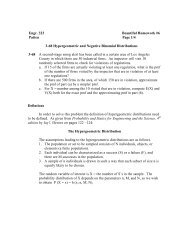
Capillary size:
50 × 2 × 0.1mm
Oxygen concentration in band:
0.3 − 0.5µM
Band width: 0.2 mm
Time of band formation:
50 sec - 3 min
Spatial assay

Capillary size:
50 × 2 × 0.1mm
Oxygen concentration in band:
0.3 − 0.5µM
Band width: 0.2 mm
Time of band formation:
50 sec - 3 min
Spatial assay

8
7
6
5
4
3
2
1
0
−1
Dashed line:path of bacteria
Solid line: turning frequency
−2
0 1 2 3 4 5 6 7 8 9 10
Time
Monte-Carlo simulation

8
7
6
5
4
3
2
1
0
−1
Dashed line:path of bacteria
Solid line: turning frequency
−2
0 1 2 3 4 5 6 7 8 9 10
Time
Monte-Carlo simulation
constant velocity, v
turning frequency
in band: σ = 0
cell leaves band
at random time, τ
outside the band
σ jumps to c
characteristic time
of adaptation: ta
adaptation: σ = ce −t−τ
ta

Modeling goals and assumptions
Goal: create a mathematical model which reproduces sharp
aerotactic band formation in spatial assays with Azospirillum
brazilense

Modeling goals and assumptions
Goal: create a mathematical model which reproduces sharp
aerotactic band formation in spatial assays with Azospirillum
brazilense
Assumptions:
• bacterial swimming is one-dimensional
and it has constant velocity

Modeling goals and assumptions
Goal: create a mathematical model which reproduces sharp
aerotactic band formation in spatial assays with Azospirillum
brazilense
Assumptions:
• bacterial swimming is one-dimensional
and it has constant velocity
• no bacterial reproduction

Modeling goals and assumptions
Goal: create a mathematical model which reproduces sharp
aerotactic band formation in spatial assays with Azospirillum
brazilense
Assumptions:
• bacterial swimming is one-dimensional
and it has constant velocity
• no bacterial reproduction
• oxygen concentration is fixed at the open end of the capillary

Modeling goals and assumptions
Goal: create a mathematical model which reproduces sharp
aerotactic band formation in spatial assays with Azospirillum
brazilense
Assumptions:
• bacterial swimming is one-dimensional
and it has constant velocity
• no bacterial reproduction
• oxygen concentration is fixed at the open end of the capillary
• no slow adaptation

∂r
∂t
∂l
∂t
Our model
= −v ∂r
∂x − frlr + flrl
= v ∂l
∂x + frlr − flrl

∂r
∂t
∂l
∂t
Our model
= −v ∂r
∂x − frlr + flrl
= v ∂l
∂x + frlr − flrl
∂L
∂t = D∂2 L
− k(r + l)
∂x2

∂r
∂t
∂l
∂t
Our model
= −v ∂r
∂x − frlr + flrl
= v ∂l
∂x + frlr − flrl
∂L
∂t = D∂2 L
− k(r + l)
∂x2 r(0, t) = l(0, t)
r(l, t) = l(l, t)
L(0, t) = L0
∂L
�
�
� = 0
∂x x=l

Proton Motive Force (PMF)
High left−to−right
turning rate
~
Lmin No turning
L min
L max
~
Lmax Turning rates
High right−to−left
turning rate

Proton Motive Force (PMF)
High left−to−right
turning rate
~
Lmin No turning
L min
L max
~
Lmax Turning rates
High right−to−left
turning rate
~
L max
L max
L min
~
L min
C c c C
C C c c
C
C
flr
frl

Proton Motive Force (PMF)
High left−to−right
turning rate
~
Lmin No turning
L min
L max
frl =
~
Lmax Turning rates
High right−to−left
turning rate
⎧
⎪⎨
⎪⎩
~
L max
L max
L min
~
L min
C c c C
C C c c
C, L < ˜ Lmin
c, ˜ Lmin < L < Lmin
c, Lmin < L < Lmax
C, Lmax < L < ˜ Lmax
C, ˜ Lmax < L
C
C
flr
frl

Parameters and nondimensionalization
Measurement Dim. quantity Non-dim. value
Length 2 mm 1
Time 10 sec 1
Oxygen conc. 1 µM
Bacterial conc.
ml
2 · 10
1
7cells
Speed
ml
40
1
µm
0.2
sec
−9 m2
sec
Diffusion coeff. 2 · 10 0.01
Turning frequency 1sec−1 10
4 · 10−3 Rate of O2 consump. 3 · 10 −11 µM
(cell)(sec)

Numerical results
Invasion of oxygen: x � √ Dt, Escape of bacteria: x � vt

Numerical results
Invasion of oxygen: x � √ Dt, Escape of bacteria: x � vt
t � D
v 2 � 5 sec, x � vt0 � 100µm → ∆x = 50µm, ∆t = 0.01

2.5
2
1.5
1
0.5
Bacteria: solid line, oxygen: dotted line, t=0 s
0
0 5 10 15 20 25 30 35 40
Numerical results
Invasion of oxygen: x � √ Dt, Escape of bacteria: x � vt
t � D
v 2 � 5 sec, x � vt0 � 100µm → ∆x = 50µm, ∆t = 0.01

2.5
2
1.5
1
0.5
Bacteria: solid line, oxygen: dotted line, t=0 s
0
0 5 10 15 20 25 30 35 40
Numerical results
0
0 5 10 15 20 25 30 35 40
Invasion of oxygen: x � √ Dt, Escape of bacteria: x � vt
t � D
v 2 � 5 sec, x � vt0 � 100µm → ∆x = 50µm, ∆t = 0.01
3.5
3
2.5
2
1.5
1
0.5
Bacteria: solid line, oxygen: dotted line, t=5 s

7
6
5
4
3
2
1
Bacteria: solid line, oxygen: dotted line, t=15 s
0
0 5 10 15 20 25 30 35 40

7
6
5
4
3
2
1
Bacteria: solid line, oxygen: dotted line, t=15 s
0
0 5 10 15 20 25 30 35 40
14
12
10
8
6
4
2
Bacteria: solid line, oxygen: dotted line, t=50 s
0
0 5 10 15 20 25 30 35 40

7
6
5
4
3
2
1
Bacteria: solid line, oxygen: dotted line, t=15 s
0
0 5 10 15 20 25 30 35 40
18
16
14
12
10
8
6
4
2
Bacteria: solid line, oxygen: dotted line, t=180 s
0
0 5 10 15 20 25 30 35 40
14
12
10
8
6
4
2
Bacteria: solid line, oxygen: dotted line, t=50 s
0
0 5 10 15 20 25 30 35 40

Numerical experiments with ˜ Lmax and ˜ Lmin
10
8
6
4
2
10
8
6
4
2
~
L max
~
L max
=4%
=7%
~
Lmin
=0%
0.5 1 1.5 2
~
Lmin
=0.5%
~
Lmin
=0%
~
L max
=7%
0.5 1 1.5 2

10
9
8
7
6
5
4
3
2
1
d
Quasi steady state solution
h
0.5 1 1.5 2
B
b 0
� L0
kb0
• d ≈
d ≈ 0.8 mm for L0 = 0.2 and
d ≈ 1.7 mm for L0 = 1
• h ≈ 2Lmax
�
kb0
kb0 L0
h ≈ 0.4mm for L0 = 0.2 and
h ≈ 0.2mm for L0 = 1

Summary of results
• model supports the notion of a novel gradient sensing mechanism

Summary of results
• model supports the notion of a novel gradient sensing mechanism
• distance between the band and the meniscus, d is predicted to
depend on external oxygen concentration, L0

Summary of results
• model supports the notion of a novel gradient sensing mechanism
• distance between the band and the meniscus, d is predicted to
depend on external oxygen concentration, L0
• width of bacterial band, h, is independent of L0 in steady state and
dependent on L0 in the quasi steady state

Summary of results
• model supports the notion of a novel gradient sensing mechanism
• distance between the band and the meniscus, d is predicted to
depend on external oxygen concentration, L0
• width of bacterial band, h, is independent of L0 in steady state and
dependent on L0 in the quasi steady state
• numerical values of d, h, bacterial density and time of pattern
formation agrees with experimental values

Summary of results
• model supports the notion of a novel gradient sensing mechanism
• distance between the band and the meniscus, d is predicted to
depend on external oxygen concentration, L0
• width of bacterial band, h, is independent of L0 in steady state and
dependent on L0 in the quasi steady state
• numerical values of d, h, bacterial density and time of pattern
formation agrees with experimental values
• model allows estimates for ˜ Lmax and ˜ Lmin which are experimentally
difficult to obtain

Slow adaptation
Fast adapation
Chemotactic models
Keller−Segel equation
Advection equation
Small spatial gradient
No tractable model
Our model
Large spatial gradient

z
z
Receptor model
Taylor and Johnson
(1998)
fast
slow
PMF
PMF

Thank you!
Bori Mazzag
Mathematics Department
Humboldt State University
1 Harpst St, Arcata CA 95521
(707) - 826 5349
bcm9@humboldt.edu

Equilibrium position for fast moving part: ˜zf = z0 f + c1p
For slow moving part: ˜zs = z0 s + c1p = z0 f − ∆z + c1p
Proton motive force: p = ±kt + c0

Equilibrium position for fast moving part: ˜zf = z0 f + c1p
For slow moving part: ˜zs = z0 s + c1p = z0 f − ∆z + c1p
Proton motive force: p = ±kt + c0
System of equations describing position of parts:
dzs
dt
zf ≈ ˜zf(p(t))
= 1
τ (˜zs(p(t) − zs)

Equilibrium position for fast moving part: ˜zf = z0 f + c1p
For slow moving part: ˜zs = z0 s + c1p = z0 f − ∆z + c1p
Proton motive force: p = ±kt + c0
System of equations describing position of parts:
Solution:
dzs
dt
zf ≈ ˜zf(p(t))
= 1
τ (˜zs(p(t) − zs)
zf = z 0 f + c0c1 ± c1kt
zs = z 0 f + c1c0 − ∆z ± c1k(t − τ) + z0e −t/τ
z 0 f : ground state (fast) z0 s: ground state (slow) τ: adaptation time