Surface-consistent Gabor deconvolution
Surface-consistent Gabor deconvolution
Surface-consistent Gabor deconvolution

Create successful ePaper yourself
Turn your PDF publications into a flip-book with our unique Google optimized e-Paper software.
<strong>Surface</strong>-<strong>consistent</strong><br />
<strong>Surface</strong> <strong>consistent</strong><br />
<strong>Gabor</strong> <strong>deconvolution</strong><br />
Carlos A. Montaña, Monta , Gary F. Margrave,<br />
and Dave Henley
Outline<br />
Why could we need SCGABOR?<br />
Overview of <strong>Gabor</strong> <strong>deconvolution</strong><br />
A surface <strong>consistent</strong> <strong>Gabor</strong><br />
algorithm<br />
Example<br />
Conclusions
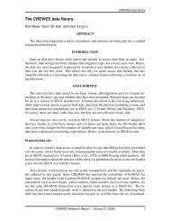
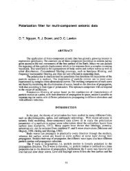
DIVETSCO TESTS<br />
(From Perz et al., 2005, CSEG meeting)
Outline<br />
Why could we need SCGABOR?<br />
Overview of <strong>Gabor</strong> <strong>deconvolution</strong><br />
A surface <strong>consistent</strong> <strong>Gabor</strong><br />
algorithm<br />
Example<br />
Conclusions
t<br />
From Wiener to <strong>Gabor</strong><br />
1. Constant Q theory 3. <strong>Gabor</strong> transform<br />
W matrix Q matrix r s<br />
τ τ<br />
t<br />
G<br />
τ t<br />
[] s ( τ , f ) ∫<br />
2. Nonstationary convolutional model<br />
<br />
s(<br />
f )<br />
∞<br />
− 2π<br />
ift<br />
= s ( t ) g ( t − τ ) e dt<br />
− ∞<br />
∞<br />
<br />
−2πifτ<br />
= w(<br />
f ) ∫α<br />
Q(<br />
f , τ ) r(<br />
τ ) e dτ<br />
−∞
Fourier of<br />
the<br />
wavelet<br />
<strong>Gabor</strong> of<br />
the trace<br />
Nonstationary conv. conv.<br />
Model<br />
in the <strong>Gabor</strong> domain<br />
Factorization of the nonstationary<br />
convolutional model<br />
<br />
s(<br />
f<br />
)<br />
∞<br />
<br />
−2πifτ<br />
= w(<br />
f ) ∫α<br />
Q ( f , τ ) r(<br />
τ ) e dτ<br />
−∞<br />
Approximated<br />
factorization<br />
<br />
G Q τ<br />
[] s ( τ , f ) ≈ w(<br />
f ) α ( τ , f ) G[]<br />
r ( , f )<br />
≈<br />
Attenuation<br />
function<br />
<strong>Gabor</strong> of the<br />
reflectivity
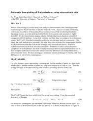
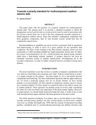
<strong>Gabor</strong> <strong>deconvolution</strong><br />
Time<br />
<strong>Gabor</strong> transform of the trace<br />
Frequency<br />
Deconvolutional operator:<br />
- smoothing<br />
-phase:<br />
using Hilbert<br />
transform<br />
Estimate of the<br />
<strong>Gabor</strong> reflectivity<br />
Wavelet removal and compensation for attenuation are simultaneous
Φ(f)<br />
Minimum phase, linearity,<br />
causality and Hilbert<br />
transform.<br />
Minimum phase<br />
– Explosive sources<br />
are also minimum<br />
phase.<br />
f<br />
A(f)<br />
=H(log( )<br />
f<br />
Futterman (1962) showed that<br />
wave attenuation in a causal,<br />
linear theory is always<br />
minimum phase.
Outline<br />
Why could we need SCGABOR?<br />
Overview of <strong>Gabor</strong> <strong>deconvolution</strong><br />
A surface <strong>consistent</strong> <strong>Gabor</strong><br />
algorithm<br />
Example<br />
Conclusions
=<br />
)<br />
( t<br />
σ<br />
σ(t)<br />
<strong>Surface</strong> Consistency<br />
<strong>Surface</strong> Consistency<br />
)<br />
,<br />
(<br />
)<br />
,<br />
( t<br />
s<br />
a<br />
t<br />
s =<br />
σ<br />
)<br />
,<br />
(<br />
)<br />
,<br />
(<br />
)<br />
,<br />
(<br />
)<br />
,<br />
(<br />
)<br />
,<br />
,<br />
,<br />
,<br />
(<br />
)<br />
,<br />
(<br />
)<br />
,<br />
(<br />
)<br />
,<br />
(<br />
)<br />
,<br />
(<br />
)<br />
,<br />
,<br />
,<br />
,<br />
(<br />
ω<br />
ω<br />
ω<br />
ω<br />
ω<br />
σ<br />
σ<br />
h<br />
D<br />
x<br />
C<br />
r<br />
B<br />
s<br />
A<br />
h<br />
x<br />
r<br />
s<br />
t<br />
h<br />
d<br />
t<br />
x<br />
c<br />
t<br />
r<br />
b<br />
t<br />
s<br />
a<br />
t<br />
h<br />
x<br />
r<br />
s<br />
=<br />
⊗<br />
⊗<br />
⊗<br />
=<br />
<br />
s<br />
)<br />
,<br />
(<br />
)<br />
,<br />
(<br />
)<br />
,<br />
,<br />
( t<br />
r<br />
b<br />
t<br />
s<br />
a<br />
t<br />
r<br />
s ⊗<br />
=<br />
σ<br />
r<br />
)<br />
,<br />
(<br />
)<br />
,<br />
(<br />
)<br />
,<br />
(<br />
)<br />
,<br />
,<br />
,<br />
( t<br />
x<br />
c<br />
t<br />
r<br />
b<br />
t<br />
s<br />
a<br />
t<br />
x<br />
r<br />
s ⊗<br />
⊗<br />
=<br />
σ<br />
x<br />
)<br />
,<br />
(<br />
)<br />
,<br />
(<br />
)<br />
,<br />
(<br />
)<br />
,<br />
(<br />
)<br />
,<br />
,<br />
,<br />
,<br />
( t<br />
h<br />
d<br />
t<br />
x<br />
c<br />
t<br />
r<br />
b<br />
t<br />
s<br />
a<br />
t<br />
h<br />
x<br />
r<br />
s ⊗<br />
⊗<br />
⊗<br />
=<br />
σ<br />
h
<strong>Surface</strong>-<strong>consistent</strong> <strong>Surface</strong> <strong>consistent</strong> <strong>Gabor</strong><br />
<strong>deconvolution</strong><br />
<br />
G[] ( τ , f ) ≈ w(<br />
f ) α ( τ , f ) G[]<br />
Q ρ ( τ , f )<br />
σ<br />
≈<br />
[ w ( f , s)<br />
][ α ( f , τ , h)<br />
][ Gρ(<br />
f , τ , h)<br />
][ w ( f , ) ]<br />
G s<br />
Q<br />
r<br />
σ ( f , τ , h,<br />
r,<br />
s)<br />
=<br />
r<br />
h, r, s: midpoint, receiver and source coordinates respectively
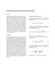
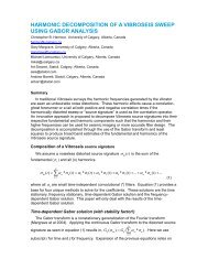
<strong>Surface</strong>-<strong>consistent</strong> <strong>Surface</strong> <strong>consistent</strong> <strong>Gabor</strong> algorithm<br />
For the i, j, k trace: ith midpoint, jth receiver and kth source indexes<br />
≈<br />
s 1 s 2 s 3 … s k .. s Ns w<br />
Sources array<br />
r 1 r 2 r 3 … r i .. r Nr<br />
Receivers array<br />
h 1 h 2 h 3 … h i .. h Nm<br />
Midpoints array
<strong>Surface</strong>-<strong>consistent</strong> <strong>Surface</strong> <strong>consistent</strong> <strong>Gabor</strong> algorithm<br />
For the i, j, k trace: ith midpoint, jth receiver and kth source indexes<br />
≈<br />
s 1 s 2 s 3 … s k .. s Ns<br />
( w )<br />
s<br />
r 1 r 2 r 3 … r i .. r Nr<br />
j<br />
=<br />
M j<br />
∑<br />
m=<br />
1<br />
w ( f , s )<br />
s<br />
M<br />
j<br />
m<br />
j<br />
( w )<br />
r<br />
k<br />
N k<br />
∑<br />
n=<br />
wr<br />
f rn<br />
=<br />
N<br />
1<br />
( , )<br />
k<br />
ijk<br />
k<br />
m 1 m 2 m 3 … m i .. m Nm<br />
Li<br />
∑<br />
l=<br />
i<br />
Ai<br />
=<br />
f x<br />
L<br />
1<br />
α(<br />
, τ ,<br />
i<br />
[ ( w ) ] . ( w )<br />
θ<br />
( f , τ ) = A * * *<br />
l i<br />
s<br />
j<br />
[ ]<br />
r<br />
k
Outline<br />
Why could we need SCGABOR?<br />
Overview of <strong>Gabor</strong> <strong>deconvolution</strong><br />
A surface <strong>consistent</strong> <strong>Gabor</strong><br />
algorithm<br />
Example<br />
Conclusions
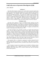
Synthetic raw data<br />
(Courtesy DIVESTCO)<br />
The dataset is made up of 78 shots,<br />
96 channels per shot<br />
Q=40, sample rate=2ms, length=2 sec.<br />
Station interval=34 m.<br />
Brute stack
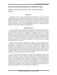
Synthetic raw data<br />
(Courtesy DIVESTCO)<br />
Q=40<br />
⊗<br />
s<br />
⊗<br />
r<br />
V=3500<br />
Strong attenuation Surf. Consist. wavelets Strong random noise
After single channel <strong>Gabor</strong>
After Surf. Cons. <strong>Gabor</strong>
Conclusions<br />
A poor S/N could harm the estimation of the<br />
minimum phase <strong>Gabor</strong> <strong>deconvolution</strong> operator,<br />
introducing undesirables artefacts<br />
The <strong>Surface</strong>-Consistent <strong>Surface</strong> Consistent implementation of<br />
<strong>Gabor</strong> <strong>deconvolution</strong> allows a robust estimation<br />
of the minimum phase <strong>deconvolution</strong> operator<br />
in the presence of<br />
– Strong random noise<br />
– Strong variations of the near-surface near surface features
Acknowledgements<br />
CREWES sponsors<br />
POTSI sponsors<br />
MITACS<br />
NSERC<br />
Mike Perz