Chernoff bound, Cramer's Theorem

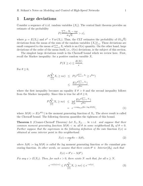
R. Srikant’s Notes on Modeling and Control of High-Speed Networks 1
1 Large deviations
Consider a sequence of i.i.d. random variables {Xi}. The central limit theorem provides an
estimate of the probability
ni=1 Xi − nµ
P (
σ √ > x),
n
where µ = E(X1) and σ 2 = V ar(X1). Thus, the CLT estimates the probability of O( √ n)
deviations from the mean of the sum of the random variables {Xi} n i=1. These deviations are
small compared to the mean of n i=1 Xi which is an O(n) quantity. On the other hand, large
deviations of the order of the mean itself, i.e., O(n) deviations, is the subject of this section.
The simplest large deviations result is the Chernoff bound which we review here. First,
recall the Markov inequality: for a positive random varaible X,
For θ ≥ 0,
P (
n
i=1
P (X ≥ ɛ) ≤ E(X)
.
ɛ
Xi ≥ nx) ≤ P (e θ n
i=1 Xi ≥ e θnx )
≤ E(eθ n i=1 Xi )
eθnx .
where the first inequality becomes an equality if θ > 0 and the second inequality follows
from the Markov inequality. Since this is true for all θ ≥ 0,
P (
n
i=1
Xi ≥ nx) ≤ inf
θ≥0
E(e θ n
i=1 Xi )
e θnx
= e −n sup θ≥0 {θx−log M(θ)} , (1)
where M(θ) := E(e θX1 ) is the moment generating function of X1. The above result is called
the Chernoff bound. The following theorem quantifies the tightness of this bound.
Theorem 1 (Cramer-Chernoff Theorem) Let X1, X2, . . . be i.i.d. and suppose that their
common moment generating function M(θ) < ∞ all θ in some neighborhood B0 of θ = 0.
Further suppose that the supremum in the following definition of the rate function I(x) is
obtained at some interior point in this neighborhood:
I(x) = sup θx − Λ(θ), (2)
θ
where Λ(θ) := log M(θ) is called the log moment generating function or the cumulant generating
function. In other words, we assume that there exists θ ∗ ∈ Interior(B0) such that
I(x) = θ ∗ x − Λ(θ ∗ ).
Fix any x > E(X1). Then, for each ɛ > 0, there exists N such that, for all n ≥ N,
e −n(I(x)+ɛ) ≤ P (
n
Xi ≥ nx) ≤ e −nI(x) . (3)
i=1

R. Srikant’s Notes on Modeling and Control of High-Speed Networks 2
(Note: Another way to state the result of the above theorem is
1
lim
n→∞ n
log P (
n
Xi ≥ nx) = −I(x).) (4)
i=1
Proof: We first prove the upper bound and then, the lower bound.
The upper bound in (3): This follows from the Chernoff bound if we show that the value
of the supremum in (1) does not change if we relax the condition θ ≥ 0 and allow θ to take
negative values. Since e θx is a convex function of x, by Jensen’s inequality, we have
M(θ) ≥ e θµ .
If θ < 0, since x − µ > 0, then e −θ(x−µ) > 1. Thus,
Taking the logarithm of both sides yields
M(θ)e −θ(x−µ) ≥ e θµ .
θx − Λ(θ) ≤ 0.
Noting that θx − Λ(θ) = 0 when θ = 0, we have
where
sup
θ
θx − Λ(θ) = sup θx − Λ(θ).
θ≥0
The lower bound in (3): Let p(x) be the pdf of X1. Then, for any δ > 0,
n
P ( Xi ≥ nx)
i=1
=
n
n
p(xi)dxi
xi ≥ nx i=1
≥
i=1
n
n
p(xi)dxi
nx ≤ xi ≤ n(x + δ) i=1
i=1
= M n (θ∗ )
enθ∗(x+δ)
e
n
nx ≤ xi ≤ n(x + δ)
i=1
nθ∗ (x+δ)
M n (θ∗ n
p(xi)dxi
) i=1
≥ M n (θ∗ )
enθ∗(x+δ)
n e
n
nx ≤ xi ≤ n(x + δ) i=1
i=1
θ∗xip(xi) M(θ∗ ) dxi
= M n (θ∗ )
enθ∗(x+δ)
n
n
q(xi)dxi,
nx ≤ xi ≤ n(x + δ) i=1
i=1
(5)
q(y) := eθ∗ y p(y)
M(θ ∗ ) .

R. Srikant’s Notes on Modeling and Control of High-Speed Networks 3
Note that ∞
−∞ q(y)dy = 1. Thus, q(y) is a pdf. Let Y be a random variable with q(y) as its
pdf. The moment generating function of Y is given by
Thus,
∞
MY (θ) =
−∞
e θy q(y)dy = M(θ + θ∗ )
M(θ∗ .
)
E(Y ) = dMY (θ)
|θ=0 =
dθ
M ′ (θ∗ )
M(θ∗ ) .
From the assumptions of the theorem θ ∗ achieves the supremum in (2). Thus,
d
θx − log M(θ) = 0
dθ
at θ = θ∗ . From this, we obtain x = M ′ (θ∗ )
M(θ∗ . Therefore, E(Y ) = x. In other words, the pdf q(y)
)
defines a set of i.i.d. random variables Yi, each with mean x. Thus, from (5), the probability
of a large deviation of the sum n i=1 Xi can be lower bounded by probability that n i=1 Yi is
near its mean nx as follows:
By the central limit theorem,
P (nx ≤
n
P ( Xi ≥ nx) ≥ e
i=1
−nI(x) e −nθ∗ n
δ
P (nx ≤ Yi ≤ n(x + δ)).
i=1
n
Yi ≤ n(x + δ)) = P (0 ≤
i=1
Given ɛ > 0, choose N (dependent on δ) such that
and
P (nx ≤
n
i=1
ni=1(Yi − x)
√ n
Yi ≤ n(x + δ)) ≥ 1
4
≤ √ n δ) n→∞
−→ 1
2 .
e −nθ∗ δ 1
4 ≥ e−nɛ .
Thus, the theorem is proved. ⋄
Remark 1 The key idea in the proof of the above theorem is the definition of a new pdf
q(y) under which the random variable has a mean at x, instead of at µ. This changes the
nature of the deviation from the mean to a small deviation, as opposed to a large deviation
and thus, allows the use of the central limit theorem to complete the proof. Changing the pdf
from p(y) to q(y) is called a change of measure. The new distribution x
−∞ q(y)dy is called
the twisted distribution or exponentially tilted distribution. ⋄
Remark 2 The theorem is also applicable when x < E(X1). To see this, define Yi = −Xi,
and consider
n
P ( Yi > −nx).
i=1

R. Srikant’s Notes on Modeling and Control of High-Speed Networks 4
Note that M(−θ) be the moment generating function of Y. Further,
I(x) = sup
θ
θx − Λ(θ) = sup −θx − Λ(−θ).
θ
Thus, the rate function is the same for Y. Since −x > E(Y1), the theorem applies to {Yi}. ⋄
Remark 3 It should be noted that the proof of the theorem can be easily modified to yield
the following result: for any δ > 0,
1
n
lim log P nx ≤ Xi ≤ n(x + δ) = −I(x).
n→∞ n
i=1
Noting that, for small δ, P (nx ≤ n i=1 Xi ≤ n(x+δ)) can be interpreted as P ( n i=1 Xi ≈ nx),
this result states that the probability that the sum of the random variables exceeds nx is
approximately equal (up to logarithmic equivalence) to the probability that the sum is “equal”
to x. ⋄
Properties of the rate function:
Lemma 1 I(x) is a convex function.
Proof:
I(αx1 + (1 − α)x2) = sup θ(αx1 + (1 − α)x2) − Λ(θ)
θ
= sup θαx1 − αΛ(θ) + θ(1 − α)x2 − (1 − α)Λ(θ)
θ
≤ sup
θ
θαx1 − αΛ(θ) + sup θ(1 − α)x2 − (1 − α)Λ(θ)
θ
= αI(x1) + (1 − α)I(x2).
Lemma 2 Let I(x) be the rate function of a random variable X with mean µ. Then,
Proof: Recall that
Thus,
By Jensen’s inequality,
Thus,
⇒
I(x) ≥ I(µ) = 0.
I(x) = sup θx − Λ(θ).
θ
I(x) ≥ 0 · x − Λ(0) = 0.
M(θ) = E(e θX ) ≥ e θµ .
Λ(θ) = log M(θ) ≥ θµ,
θµ − Λ(θ) ≤ 0
⇒
I(µ) = sup θµ − Λ(θ) ≤ 0.
θ
Since we have shown that I(x) ≥ 0 ∀x, we have the desired result. ⋄
⋄

R. Srikant’s Notes on Modeling and Control of High-Speed Networks 5
Lemma 3
Λ(θ) = sup θx − I(x).
x
Proof: We will prove this under the assumption that all functions of interest are differentiable.
From the definition of I(x) and the convexity of Λ(θ),
where θ ∗ solves
I(x) = θ ∗ x − Λ(θ ∗ ), (6)
Λ ′ (θ ∗ ) = x. (7)
Since I(x) is convex, it is enough to show that, for each θ, there exists an x ∗ such that
Λ(θ) = θx ∗ − I(x ∗ ) (8)
and θ = I ′ (x ∗ ). We claim that such an x ∗ is given by x ∗ = Λ ′ (θ). To see this, we note from
(6)-(7) that
I(x ∗ ) = θx ∗ − Λ(θ)
which verifies (8). ⋄