Chapter 5. The Second Fundamental Form
Chapter 5. The Second Fundamental Form
Chapter 5. The Second Fundamental Form

Create successful ePaper yourself
Turn your PDF publications into a flip-book with our unique Google optimized e-Paper software.
<strong>Chapter</strong> <strong>5.</strong> <strong>The</strong> <strong>Second</strong> <strong>Fundamental</strong> <strong>Form</strong><br />
Directional Derivatives in IR 3 .<br />
Let f : U ⊂ IR 3 → IR be a smooth function defined on an open subset of IR 3 .<br />
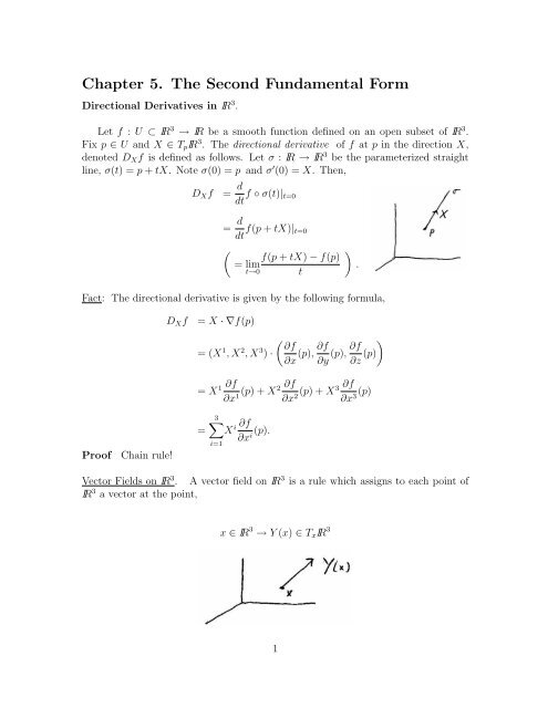
Fix p ∈ U and X ∈ TpIR 3 . <strong>The</strong> directional derivative of f at p in the direction X,<br />
denoted DXf is defined as follows. Let σ : IR → IR 3 be the parameterized straight<br />
line, σ(t) = p + tX. Note σ(0) = p and σ ′ (0) = X. <strong>The</strong>n,<br />
DXf = d<br />
f ◦ σ(t)|t=0<br />
dt<br />
= d<br />
f(p + tX)|t=0<br />
dt<br />
<br />
<br />
f(p + tX) − f(p)<br />
= lim<br />
.<br />
t→0 t<br />
Fact: <strong>The</strong> directional derivative is given by the following formula,<br />
Proof Chain rule!<br />
DXf = X · ∇f(p)<br />
= (X 1 , X 2 , X 3 ) ·<br />
= X<br />
=<br />
<br />
∂f ∂f ∂f<br />
(p), (p),<br />
∂x ∂y ∂z (p)<br />
<br />
1 ∂f ∂f ∂f<br />
(p) + X2 (p) + X3<br />
∂x1 ∂x2 ∂x<br />
3<br />
X<br />
i=1<br />
i ∂f<br />
(p).<br />
∂xi Vector Fields on IR 3 . A vector field on IR 3 is a rule which assigns to each point of<br />
IR 3 a vector at the point,<br />
x ∈ IR 3 → Y (x) ∈ TxIR 3<br />
1<br />
3 (p)
Analytically, a vector field is described by a mapping of the form,<br />
Y : U ⊂ IR 3 → IR 3 ,<br />
Y (x) = (Y 1 (x), Y 2 (x), Y 3 (x)) ∈ TxIR 3 .<br />
Components of Y : Y i : U → IR, i = 1, 2, 3.<br />
Ex. Y : IR 3 → IR 3 , Y (x, y, z) = (y + z, z + x, x + y). E.g., Y (1, 2, 3) = (5, 4, 3), etc.<br />
Y 1 = y + z, Y 2 = z + x, and Y 3 = x + y.<br />
<strong>The</strong> directional derivative of a vector field is defined in a manner similar to the<br />
directional derivative of a function: Fix p ∈ U, X ∈ TpIR 3 . Let σ : IR → IR 3 be the<br />
parameterized line σ(t) = p + tX (σ(0) = p, σ ′ (0) = X). <strong>The</strong>n t → Y ◦ σ(t) is a<br />
vector field along σ in the sense of the definition in <strong>Chapter</strong> 2. <strong>The</strong>n, the directional<br />
derivative of Y in the direction X at p, is defined as,<br />
DXY = d<br />
Y ◦ σ(t)|t=0<br />
dt<br />
I.e., to compute DXY , restrict Y to σ to obtain a vector valued function of t, and<br />
differentiate with respect to t.<br />
In terms of components, Y = (Y 1 , Y 2 , Y 3 ),<br />
DXY = d<br />
dt (Y 1 ◦ σ(t), Y 2 ◦ σ(t), Y 3 ◦ σ(t))|t=0<br />
<br />
d<br />
=<br />
dt Y 1 ◦ σ(t)|t=0 , d<br />
dt Y 2 ◦ σ(t)|t=0 , d<br />
dt Y 3 <br />
◦ σ(t)|t=0<br />
= (DXY 1 , DXY 2 , DXY 3 ).<br />
2
Directional derivatives on surfaces.<br />
Let M be a surface, and let f : M → IR be a smooth function on M. Recall, this<br />
means that ˆ f = f ◦ x is smooth for all proper patches x : U → M in M.<br />
Def. For p ∈ M, X ∈ TpM, the directional derivative of f at p in the direction X,<br />
denoted ∇Xf, is defined as follows. Let σ : (−ɛ, ɛ) → M ⊂ IR 3 be any smooth curve<br />
in M such that σ(0) = p and σ ′ (0) = X. <strong>The</strong>n,<br />
∇Xf = d<br />
f ◦ σ(t)|t=0<br />
dt<br />
I.e., to compute ∇Xf, restrict f to σ and differentiate with respect to parameter t.<br />
Proposition. <strong>The</strong> directional derivative is well-defined, i.e. independent of the<br />
particular choice of σ.<br />
Proof. Let x : U → M be a proper patch containing p. Express σ in terms of<br />
coordinates in the usual manner,<br />
By the chain rule,<br />
σ(t) = x(u 1 (t), u 2 (t)) .<br />
dσ<br />
dt = dui<br />
dt xi<br />
<br />
xi = ∂x<br />
<br />
∂ui<br />
X ∈ TpM ⇒ X = Xixi. <strong>The</strong> initial condition, dσ<br />
(0) = X then implies<br />
dt<br />
Now,<br />
du i<br />
dt (0) = Xi , i = 1, 2.<br />
f ◦ σ(t) = f(σ(t)) = f(x(u 1 (t), u 2 (t))<br />
= f ◦ x(u 1 (t), u 2 (t))<br />
= ˆ f(u 1 (t), u 2 (t)).<br />
3
Hence, by the chain rule,<br />
<strong>The</strong>refore,<br />
or simply,<br />
d<br />
dt f ◦ σ(t) = ∂ ˆ f<br />
∂u1 du1 dt + ∂ ˆ f<br />
∂u2 du2 dt<br />
= ∂ ˆ f<br />
∂ui ∇Xf = d<br />
f ◦ σ(t)|t=0<br />
dt<br />
= <br />
i<br />
i<br />
du i<br />
dt<br />
= <br />
i<br />
du i<br />
dt<br />
∂ ˆ f<br />
.<br />
∂ui du i<br />
dt (0) ∂ ˆ f<br />
∂u i (u1 , u 2 ) , (p = x(u 1 , u 2 ))<br />
∇Xf = <br />
Xi ∂ ˆ f<br />
∂ui (u1 , u2 ) ,<br />
i<br />
∇Xf = X i ∂ ˆ f<br />
∂u i<br />
= X1 ∂ ˆ f<br />
∂u1 + X2 ∂ ˆ f<br />
. (∗)<br />
∂u2 Ex. Let X = x1. Since x1 = 1 · x1 + 0 · x2, X1 = 1 and X2 = 0. Hence the above<br />
equation implies, ∇x1f = ∂ ˆ f<br />
∂u1 . Similarly, ∇x2f = ∂ ˆ f<br />
. I.e.,<br />
∂u2 ∇xif = ∂ ˆ f<br />
, i = 1, 2.<br />
∂ui <strong>The</strong> following proposition summarizes some basic properties of directional derivatives<br />
in surfaces.<br />
Proposition<br />
(1) ∇(aX+bY )f = a∇Xf + b∇Y f<br />
(2) ∇X(f + g) = ∇Xf + ∇Xg<br />
(3) ∇Xfg = (∇Xf)g + f(∇Xg)<br />
4
Exercise <strong>5.</strong>1. Prove this proposition.<br />
Vector fields along a surface.<br />
A vector field along a surface M is a rule which assigns to each point of M a<br />
vector at that point,<br />
N.B. Y (x) need not be tangent to M.<br />
x ∈ M → Y (x) ∈ TxIR 3<br />
Analytically vector fields along a surface M are described by mappings.<br />
Y : M → IR 3<br />
Y (x) = (Y 1 (x), Y 2 (x), Y 3 (x)) ∈ TxIR 3<br />
Components of Y : Y i : M → IR, i = 1, 2, 3. We say Y is smooth if its component<br />
functions are smooth.<br />
<strong>The</strong> directional derivative of a vector field along M is defined in a manner similar<br />
to the directional derivative of a function defined on M.<br />
Given a vector field along M, Y : M → IR 3 , for p ∈ M, X ∈ TpM, the directional<br />
derivative of Y in the direction X, denoted ∇XY , is defined as,<br />
∇XY = d<br />
Y ◦ σ(t)|t=0<br />
dt<br />
where σ : (−ɛ, ɛ) → M is a smooth curve in M such that σ(0) = p and dσ<br />
(0) = X.<br />
dt<br />
5
I.e. to compute ∇XY , restrict Y to σ to obtain a vector valued function of t - then<br />
differentiate with respect to t.<br />
Fact If Y (x) = (Y 1 (x), Y 2 (x), Y 3 (x)) then,<br />
Proof: Exercise.<br />
∇XY = (∇XY 1 , ∇XY 2 , ∇XY 3 )<br />
Surface Coordinate Expression. Let x : U → M be a proper patch in M containing<br />
p. Let X ∈ TpM, X = <br />
xixi. An argument like that for functions on M shows,<br />
i<br />
∇XY =<br />
2<br />
i=1<br />
X i ∂ ˆ Y<br />
∂u i (u1 , u 2 ) , (p = x(u 1 , u 2 ))<br />
where ˆ Y = Y ◦ x : U → IR 3 is Y expressed in terms of coordinates.<br />
Exercise <strong>5.</strong>2. Derive the expression above for ∇XY . In particular, show<br />
∇xiY = ∂ ˆ Y<br />
, i = 1, 2 .<br />
∂ui Some basic properties are described in the following proposition.<br />
Proposition<br />
(1) ∇aX+bY Z = a∇XZ + b∇Y Z<br />
(2) ∇X(Y + Z) = ∇XY + ∇XZ<br />
(3) ∇X(fY ) = (∇Xf)Y + f∇XY<br />
(4) ∇X〈Y, Z〉 = 〈∇XY, Z〉 + 〈Y, ∇XZ〉<br />
6
<strong>The</strong> Weingarten Map and the 2nd <strong>Fundamental</strong> <strong>Form</strong>.<br />
We are interested in studying the shape of surfaces in IR 3 . Our approach (essentially<br />
due to Gauss) is to study how the unit normal to the surface “wiggles” along<br />
the surface.<br />
<strong>The</strong> objects which describe the shape of M are:<br />
1. <strong>The</strong> Weingarten Map, or shape operator. For each p ∈ M this is a certain linear<br />
transformation L : TpM → TpM.<br />
2. <strong>The</strong> second fundamental form. This is a certain bilinear form L : TpM ×TpM →<br />
IR associated in a natural way with the Weingarten map.<br />
We now describe the Weingarten map. Fix p ∈ M. Let n : W → IR 3 , p ∈ W →<br />
n(p) ∈ TpIR 3 , be a smooth unit normal vector field defined along a neighborhood W<br />
of p.<br />
Remarks<br />
1. n can always be constructed by introducing a proper patch x : U → M, x =<br />
x(u 1 , u 2 ) containing p:<br />
ˆn = x1 × x2<br />
|x1 × x2| ,<br />
ˆn : U → IR 3 , ˆn = ˆn(u 1 , u 2 ). <strong>The</strong>n, n = ˆn ◦ x −1 : x(U) → IR 3 is a smooth unit normal<br />
v.f. along x(U).<br />
2. <strong>The</strong> choice of n is not quite unique: n → −n; choice of n is unique “up to sign”<br />
7
3. A smooth unit normal field n always exists in a neighborhood of any given point<br />
p, but it may not be possible to extend n to all of M. This depends on whether or<br />
not M is an orientable surface.<br />
Ex. Möbius band.<br />
Lemma. Let M be a surface, p ∈ M, and n be a smooth unit normal vector field<br />
defined along a neighborhood W ⊂ M of p. <strong>The</strong>n for any X ∈ TpM, ∇Xn ∈ TpM.<br />
Proof. It suffices to show that ∇Xn is perpendicular to n. |n| = 1 ⇒ 〈n, n〉 = 1 ⇒<br />
and hence ∇Xn ⊥ n.<br />
∇X〈n, n〉 = ∇X1<br />
〈∇Xn, n〉 + 〈n, ∇Xn〉 = 0<br />
2〈∇Xn, n〉 = 0<br />
Def. Let M be a surface, p ∈ M, and n be a smooth unit normal v.f. defined<br />
along a nbd W ⊂ M of p. <strong>The</strong> Weingarten Map (or shape operator) is the map<br />
L : TpM → TpM defined by,<br />
L(X) = −∇Xn .<br />
Remarks<br />
1. <strong>The</strong> minus sign is a convention – will explain later.<br />
2. L(X) = −∇Xn = − d<br />
n ◦ σ(t)|t=0<br />
dt<br />
8
Lemma: L : TpM → TpM is a linear map, i.e.,<br />
for all X, Y, ∈ TpM, a, b ∈ IR.<br />
L(aX + bY ) = aL(X) + bL(Y ) .<br />
Proof. Follows from properties of directional derivative,<br />
Ex. Let M be a plane in IR 3 :<br />
L(aX + bY ) = −∇aX+bY n<br />
= −[a∇Xn + b∇Y n]<br />
= a(−∇Xn) + b(−∇Y n)<br />
= aL(X) + bL(Y ).<br />
M : ax + by + cz = d<br />
Determine the Weingarten Map at each point of M. Well,<br />
(a, b, c)<br />
n = √<br />
a2 + b2 + c2 =<br />
<br />
a b c<br />
, , ,<br />
λ λ λ<br />
where λ = √ a 2 + b 2 + c 2 . Hence,<br />
L(X) = −∇Xn = −∇X<br />
<br />
= −<br />
∇X<br />
<strong>The</strong>refore L(X) = 0 ∀ X ∈ TpM, i.e. L ≡ 0.<br />
<br />
a b c<br />
, ,<br />
λ λ λ<br />
<br />
a b c<br />
, ∇X , ∇X = 0.<br />
λ λ λ<br />
Ex. Let M = S 2 r be the sphere of radius r, let n be the outward pointing unit<br />
normal. Determine the Weingarten map at each point of M.<br />
9
Fix p ∈ S 2 r , and let X ∈ TpS 2 r . Let σ : (−ε, ε) → S 2 r be a curve in S 2 r such that<br />
σ(0) = p, dσ<br />
(0) = X<br />
dt<br />
<strong>The</strong>n,<br />
But note, n ◦ σ(t) = n(σ(t)) = σ(t)<br />
|σ(t)|<br />
L(X) = −∇Xn = − d<br />
dt n ◦ σ(t)|t=0 .<br />
L(X) = − d σ(t)<br />
dt<br />
σ(t)<br />
= . Hence,<br />
r<br />
r |t=0 = − 1<br />
r<br />
dσ<br />
dt |t=0<br />
L(X) = − 1<br />
X .<br />
r<br />
for all X ∈ TpM. Hence, L = − 1<br />
r id, where id : TpM → TpM is the identity map,<br />
id(X) = X.<br />
Remark. If we had taken the inward pointing normal then L = 1<br />
r id.<br />
Def. For each p ∈ M, the second fundamental form is the bilinear form<br />
L = TpM × TpM → IR defined by,<br />
L is indeed bilinear, e.g.,<br />
Ex. M = plane, L ≡ 0:<br />
L(X, Y ) = 〈L(X), Y 〉<br />
= −〈∇Xn, Y 〉.<br />
L(aX + bY, Z) = 〈L(aX + bY ), Z〉<br />
= 〈aL(X) + bL(Y ), Z〉<br />
= a〈L(X), Z〉 + b〈L(Y ), Z〉<br />
= aL(X, Z) + bL(Y, Z).<br />
L(X, Y ) = 〈L(X), Y 〉 = 〈0, Y 〉 = 0.<br />
Ex. <strong>The</strong> sphere S 2 r of radius r, L : TpS 2 r × TpS 2 r → IR,<br />
L(X, Y ) = 〈L(X), Y 〉<br />
= 〈− 1<br />
X, Y 〉<br />
r<br />
= − 1<br />
〈X, Y 〉<br />
r<br />
10
Hence, L = − 1<br />
〈 , 〉. Multiple of the first fundamental form!<br />
r<br />
Coordinate expressions<br />
Let x : U → M be a patch containing p ∈ M. <strong>The</strong>n {x1, x2} is a basis for TpM.<br />
We express L : TpM → TpM and L : TpM × TpM → R with respect to this basis.<br />
Since L(xj) ∈ TpM, we have,<br />
L(xj) = L 1 jx1 + L 2 jx2 , j = 1, 2<br />
=<br />
2<br />
i=1<br />
L i jxi .<br />
<strong>The</strong> numbers L i j, 1 ≤ i, j ≤ 2, are called the components of L with respect to the<br />
coordinate basis {x1, x2}. <strong>The</strong> 2 × 2 matrix [L i j] is the matrix representing the linear<br />
map L with respect to the basis {x1, x2}.<br />
<br />
Exercise <strong>5.</strong>3 Let X ∈ TpM and let Y = L(X).<br />
j<br />
In terms of components, X =<br />
Xjxj and Y = <br />
i Y ixi. Show that<br />
Y i = <br />
L i jX j , i = 1, 2 ,<br />
which in turn implies the matrix equation,<br />
<br />
1 Y<br />
Y 2<br />
<br />
= L i <br />
j<br />
X1 X2 <br />
.<br />
j<br />
This is the Weingarten map expressed as a matrix equation.<br />
Introduce the unit normal field along W = x(U) with respect to the patch x :<br />
U → M,<br />
<strong>The</strong>n by Exercise <strong>5.</strong>2,<br />
Setting nj = ∂ˆn<br />
∂u j we have<br />
nj = −L(xj)<br />
nj = − <br />
i<br />
ˆn = x1 × x2<br />
|x1 × x2| , ˆn = ˆn(u1 , u 2 ) ,<br />
n = ˆn ◦ x −1 : W → R .<br />
L(xj) = −∇xj<br />
∂ˆn<br />
n = − .<br />
∂uj L i jxi , j = 1, 2 (<strong>The</strong> Weingarten equations.)<br />
11
<strong>The</strong>se equations can be used to compute the components of the Weingarten map.<br />
However, in practice it turns out to be more useful to have a formula for computing<br />
the components of the second fundamental form.<br />
Components of L:<br />
<strong>The</strong> components of L with respect to {x1, x2} are defined as,<br />
Lij = L(xi, xj) , 1 ≤ i, j ≤ 2 .<br />
By bilinearity, the components completely determine L,<br />
L(X, Y ) = L( <br />
X i xi, <br />
Y j xj)<br />
= <br />
i,j<br />
= <br />
i,j<br />
i<br />
X i Y j L(xi, xj)<br />
LijX i Y j .<br />
<strong>The</strong> following proposition provides a useful formula for computing the Lij’s.<br />
Proposition. <strong>The</strong> components Lij of L are given by,<br />
where xij = ∂2x ∂uj .<br />
∂ui Lij = 〈ˆn, xij〉 ,<br />
Remark. Henceforth we no longer distinguish between n and ˆn, i.e., lets agree to<br />
drop the “ ˆ ”, then,<br />
Lij = 〈n, xij〉 ,<br />
Proof:<br />
12<br />
j
Along x(U) we have, 〈n, ∂x<br />
∂u j 〉 = 0, and hence,<br />
∂ ∂x<br />
〈n,<br />
∂ui ∂u<br />
j 〉 = 0<br />
〈 ∂n ∂x<br />
,<br />
∂ui ∂uj 〉 + 〈n, ∂2x ∂ui 〉 = 0<br />
∂uj or, using shorthand notation,<br />
But,<br />
〈 ∂n ∂x<br />
,<br />
∂ui ∂uj 〉 = −〈n, ∂2x ∂ui∂uj 〉 = −〈n, ∂2x ∂uj 〉 ,<br />
∂ui 〈ni, xj〉 = −〈n, xij〉 .<br />
Lij = L(xi, xj) = 〈L(xi), xj〉<br />
= −〈ni, xj〉 ,<br />
and hence Lij = 〈n, xij〉. ✷<br />
Observe,<br />
In other words, L(xi, xj) = L(xj, xi).<br />
Lij = 〈n, xij〉<br />
= 〈n, xji〉 (mixed partials equal!)<br />
Lij = Lji , 1 ≤ i, j ≤ 2 .<br />
Proposition. <strong>The</strong> second fundamental form L : TpM × TpM → IR is symmetric,<br />
i.e.<br />
L(X, Y ) = L(Y, X) ∀ X, Y ∈ TpM .<br />
Exercise <strong>5.</strong>4 Prove this proposition by showing L is symmetric iff Lij = Lji for all<br />
1 ≤ i, j ≤ 2.<br />
Relationship between L i j and Lij<br />
Lij = L(xi, xj) = L(xj, xi)<br />
= 〈L(xj), xi〉 = 〈 <br />
Lk jxk, xi, 〉<br />
= <br />
Lk j〈xk, xi〉<br />
k<br />
Lij = <br />
k<br />
gikL k j, 1 ≤ i, j ≤ 2<br />
13<br />
k
Classical tensor jargon: Lij obtained from L k j by “lowering the index k with the<br />
metric”. <strong>The</strong> equation above implies the matrix equation<br />
[Lij] = [gij][L i j] .<br />
Geometric Interpretation of the 2nd <strong>Fundamental</strong> <strong>Form</strong><br />
Normal Curvature. Let s → σ(s) be a unit speed curve lying in a surface M. Let<br />
p be a point on σ, and let n be a smooth unit normal v.f. defined in a nbd W of p.<br />
<strong>The</strong> normal curvature of σ at p, denoted κn, is defined to be the component of the<br />
curvature vector σ ′′ = T ′ along n, i.e.,<br />
κn = normal component of the curvature vector<br />
= 〈σ ′′ , n〉<br />
= 〈T ′ , n〉<br />
= |T ′ | |n| cos θ<br />
= κ cos θ ,<br />
where θ is the angle between the curvature vector T ′ and the surface normal n. If<br />
κ = 0 then, recall, we can introduce the principal normal N to σ, by the equation,<br />
T ′ = κN; in this case θ is the angle beween N and n.<br />
Remark: κn gives a measure of how much σ is bending in the direction perpendicular<br />
to the surface; it neglects the amount of bending tangent to the surface.<br />
Proposition. Let M be a surface, p ∈ M. Let X ∈ TpM, |X| = 1 (i.e. X is a<br />
unit tangent vector). Let s → σ(s) be any unit speed curve in M such that σ(0) = p<br />
and σ ′ (0) = X. <strong>The</strong>n<br />
L(X, X) = normal curvature of σ at p<br />
= 〈σ ′′ , n〉.<br />
14
Proof. Along σ,<br />
At s = 0,<br />
〈σ ′ (s), n ◦ σ(s)〉 = 0 , for all s<br />
d<br />
ds 〈σ′ , n ◦ σ〉 = 0<br />
〈σ ′′ , n ◦ σ〉 + 〈σ ′ , d<br />
n ◦ σ〉 = 0 .<br />
ds<br />
〈σ ′′ , n〉 + 〈X, ∇Xn〉 = 0<br />
〈σ ′′ , n〉 = −〈X, ∇Xn〉<br />
κn = 〈X, L(X)〉<br />
κn = 〈L(X), X〉<br />
= L(X, X).<br />
Remark: the sign convention used in the definition of the Weingarten map ensures<br />
that L(X, X) = +κn (rather than −κn).<br />
Corollary. All unit speed curves lying in a surface M which pass through p ∈ M<br />
and have the same unit tangent vector X at p, have the same normal curvature at p.<br />
That is, the normal curvature depends only on the tangent direction X.<br />
Thus it makes sense to say:<br />
L(X, X) is the normal curvature in the direction X .<br />
Given a unit tangent vector X ∈ TpM, there is a distinguished curve in M, called<br />
the normal section at p in the direction X. Let,<br />
Π = plane through p spanned by n and X.<br />
Π cuts M in a curve σ. Parameterize σ wrt arc length, s → σ(s), such that σ(0) = p<br />
and dσ<br />
(0) = X :<br />
ds<br />
15
By definition, σ is the normal section at p in the direction X. By the previous<br />
proposition,<br />
L(X, X) = normal curvature of the normal section σ<br />
= 〈σ ′′ , n〉 = 〈T ′ , n〉<br />
= κ cos θ ,<br />
where θ is the angle between n and T ′ . Since σ lies in Π, T ′ is tangent to Π, and<br />
since T ′ is also perpendicular to X, it follows that T ′ is a multiple of n. Hence, θ = 0<br />
or π, which implies that L(X, X) = ±κ.<br />
Thus we conclude that,<br />
L(X, X) = signed curvature of the normal section at p in the direction X.<br />
Principal Curvatures.<br />
<strong>The</strong> set of unit tangent vectors at p, X ∈ TpM, |X| = 1, forms a circle in the<br />
tangent plane to M at p. Consider the function from this circle into the reals,<br />
X → normal curvature in direction X<br />
X → L(X, X).<br />
<strong>The</strong> principal curvatures of M at p, κ1 = κ1(p) and κ2 = κ2(p), are defined as<br />
follows,<br />
κ1 = the maximum normal curvature at p<br />
= max L(X, X)<br />
|X|=1<br />
κ2 = the minimum normal curvature at p<br />
= min L(X, X)<br />
|X|=1<br />
This is the geometric characterization of principal curvatures. <strong>The</strong>re is also an<br />
important algebraic characterization.<br />
16
Some Linear Algebra<br />
Let V be a vector space over the reals, and let 〈 , 〉 : V × V → IR be an<br />
inner product on V ; hence V is an inner product space. Let L : V → V be a linear<br />
transformation. Our main application will be to the case: V = TpM, 〈 , 〉 = induced<br />
metric, and L = Weingarten map.<br />
L is said to be self adjoint provided<br />
〈L(v), w〉 = 〈v, L(w)〉 ∀ v, w ∈ V .<br />
Remark. Let V = IR n , with the usual dot product, and let L : IR n → IR n be<br />
a linear map. Let [L i j] = matrix representing L with respect to the standard basis,<br />
e1 : (1, 0, ..., 0), etc. <strong>The</strong>n L is self-adjoint if and only if [L i j] is symmetric [L i j] = [L j i].<br />
Proposition. <strong>The</strong> Weingarten map L : TpM → TpM is self adjoint, i.e.<br />
where 〈 , 〉 = 1st fundamental form.<br />
Proof. We have,<br />
〈L(X), Y 〉 = 〈X, L(Y )〉 ∀ X, Y ∈ TpM,<br />
〈L(X), Y 〉 = L(X, Y ) = L(Y, X)<br />
= 〈L(Y ), X〉 = 〈X, L(Y )〉.<br />
Self adjoint linear transformations have very nice properties, as we now discuss.<br />
For this discussion, we restrict attention to 2-dimensional vector spaces, dim V = 2.<br />
A vector v ∈ V, v = 0, is called an eigenvector of L if there is a real number λ<br />
such that,<br />
L(v) = λv .<br />
λ is called an eigenvalue of L. <strong>The</strong> eigenvalues of L can be determined by solving<br />
det(A − λI) = 0<br />
where A is a matrix representing L and I = identity matrix. <strong>The</strong> equation (∗) is<br />
a quadratic equation in λ, and hence has at most 2 real roots; it may have no real<br />
roots.<br />
<strong>The</strong>orem (<strong>Fundamental</strong> <strong>The</strong>orem of Self Adjoint Operators) Let V be a 2-dimensional<br />
inner product space. Let L : V → V be a self-adjoint linear map. <strong>The</strong>n V admits an<br />
orthonormal basis consisting of eigenvectors of L. That is, there exists an orthonormal<br />
basis {e1, e2} of V and real numbers λ1, λ2, λ1 ≥ λ2 such that<br />
L(e1) = λ1e1, L(e2) = λ2e2,<br />
17<br />
(∗)
i.e., e1 and e2 are eigenvectors of L and λ1, λ2 are the corresponding eigenvalues.<br />
Moreover the eigenvalues are given by<br />
Proof. See handout from Do Carmo.<br />
λ1 = max〈L(v),<br />
v〉<br />
|v|=1<br />
λ2 = min〈L(v),<br />
v〉 .<br />
|v|=1<br />
Remark on orthogonality of eigenvectors. Let e1, e2 be eigenvectors with eigenvalues<br />
λ1, λ2. If λ1 = λ2, then e1 and e2 are necessarily orthogonal, as seen by the following,<br />
λ1〈e1, e2〉 = 〈L(e1), e2〉 = 〈e1, L(e2)〉 = λ2〈e1, e2〉 ,<br />
⇒ (λ1 − λ2)〈e1, e2〉 = 0 ⇒ 〈e1, e2〉 = 0. On the other hand, if λ1 = λ2 = λ then<br />
L(v) = λv for all v. Hence any o.n. basis is a basis of eigenvectors.<br />
We now apply these facts to the Weingarten map,<br />
L : TpM → TpM ,<br />
L : TpM × TpM → IR, L(X, Y ) = 〈L(X), Y 〉 .<br />
Since L is self adjoint, and, by definition,<br />
we obtain the following.<br />
κ1 = max<br />
|X|=1<br />
κ2 = min<br />
|X|=1<br />
L(X, X) = max〈L(X),<br />
X〉<br />
|X|=1<br />
L(X, X) = min 〈L(X), X〉 ,<br />
|X|=1<br />
<strong>The</strong>orem. <strong>The</strong> principal curvatures κ1, κ2 of M at p are the eigenvalues of the<br />
Weingarten map L : TpM → TpM. <strong>The</strong>re exists an orthonormal basis {e1, e2} of<br />
TpM such that<br />
L(e1) = κ1e1, L(e2) = κ2e2 ,<br />
i.e., e1, e2 are eigenvectors of L associated with the eigenvalues κ1, κ2, respectively.<br />
<strong>The</strong> eigenvectors e1 and e2 are called principal directions.<br />
Observe that,<br />
κ1 = κ1〈e1, e1〉 = 〈L(e1), e1〉 = L(e1, e1)<br />
κ2 = κ2〈e2, e2〉 = 〈L(e2), e2〉 = L(e2, e2) ,<br />
i.e., the principal curvature κ1 is the normal curvature in the principal direction e1,<br />
and similarly for κ2.<br />
18
Now, let A be the matrix associated to the Weingarten map L with respect to the<br />
orthonormal basis {e1, e2}; thus,<br />
which implies,<br />
<strong>The</strong>n,<br />
L(e1) = κ1e1 + 0e2<br />
L(e2) = 0e1 + κ2e2<br />
<br />
κ1 0<br />
A =<br />
0 κ2<br />
<br />
.<br />
det L = det A = κ1κ2<br />
tr L = tr A = κ1 + κ2 .<br />
Definition. <strong>The</strong> Gaussian curvature of M at p, K = K(p), and the mean curvature<br />
of M at p, H = H(p) are defined as follows,<br />
K = det L = κ1κ2<br />
H = tr L = κ1 + κ2 .<br />
Remarks. <strong>The</strong> Gaussian curvature is the more important of the two curvatures; it<br />
is what is meant by the curvature of a surface. A famous discovery by Gauss is that<br />
it is intrinsic – in fact can be computed in terms of the gij’s (This is not obvious!).<br />
<strong>The</strong> mean curvature (which has to do with minimal surface theory) is not intrinsic.<br />
This can be easily seen as follows. Changing the normal n → −n changes the sign of<br />
the Weingarten map,<br />
L−n = −Ln .<br />
This in turn changes the sign of the principal curvatures, hence H = κ1 + κ2 changes<br />
sign, but K = κ1κ2 does not change sign.<br />
19
Some Examples<br />
Ex. For S 2 r = sphere of radius r, compute κ1, κ2, K, H (Use outward normal).<br />
Geometrically: p ∈ S 2 r , X ∈ TpM, |X| = 1,<br />
<strong>The</strong>refore<br />
L(X, X) = ± curvature of normal section in direction X<br />
= −curvature of great circle<br />
= − 1<br />
r .<br />
κ1 = max L(X, X) = −<br />
|X|=1<br />
1<br />
r ,<br />
κ2 = min L(X, X) = −<br />
|X|=1<br />
1<br />
r ,<br />
K = κ1κ2 = 1<br />
r 2 > 0, H = κ1 + κ2 = − 2<br />
r .<br />
Algebraically: Find eigenvalues of Weingarten map: L : TpM → TpM. We showed<br />
previously,<br />
L = − 1<br />
id, i.e.,<br />
r<br />
L(X) = − 1<br />
X for all X ∈ TpM.<br />
r<br />
Thus, with respect to any orthonormal basis {e1, e2} of TpM,<br />
L(ei) = − 1<br />
r ei i = 1, 2.<br />
20
<strong>The</strong>refore, κ1 = κ2 = − 1 1<br />
, K = , H = −2<br />
r r2 r .<br />
Ex. Let M be the cylinder of radius a: x 2 + y 2 = a 2 . Compute κ1, κ2, K, H. (Use<br />
the inward pointing normal)<br />
Geometrically:<br />
L(X1, X1) = ± curvature of normal section in direction X1<br />
= + curvature of circle of radius a<br />
= 1<br />
a ,<br />
L(X2, X2) = ± curvature of normal section in direction X2<br />
= curvature of line<br />
= 0 .<br />
In general, for X = X1, X2,<br />
L(X, X) = curvature of ellipse through p .<br />
<strong>The</strong> curvature is between 0 and 1,<br />
and thus,<br />
a<br />
0 ≤ L(X, X) ≤ 1<br />
a .<br />
21
We conclude that,<br />
κ1 = max L(X, X) = L(X1, X1) =<br />
|X|=1<br />
1<br />
a ,<br />
κ2 = min L(X, X) = L(X2, X2) = 0 .<br />
|X|=1<br />
Thus, K = 0 (cylinder is flat!) and H = 1<br />
a .<br />
Algebraically: Determine the eigenvalues of the Weingarten map. By a rotation and<br />
translation we may take p to be the point p = (a, 0, 0). Let e1, e2 ∈ TpM be the<br />
tangent vectors e1 = (0, 1, 0) and e2 = (0, 0, 1).<br />
To compute L(e1), consider the circle,<br />
Note that σ(0) = p and σ ′ (0) = e1. Thus,<br />
. But,<br />
σ(s) = (a cos( s s<br />
), a sin( ), 0)<br />
a a<br />
L(e1) = −∇e1n<br />
= − d<br />
ds n(σ(s))|s=0<br />
n(σ(s)) = n(σ(s)) = σ(s) σ(s)<br />
=<br />
|σ(s)| a<br />
=<br />
<br />
s<br />
<br />
s<br />
<br />
− cos , sin , 0<br />
a a<br />
22
<strong>The</strong>refore,<br />
L(e1) = d<br />
<br />
cos<br />
ds<br />
= 1<br />
<br />
− sin<br />
a<br />
= 1<br />
(0, 1, 0)<br />
a<br />
L(e1) = 1<br />
a e1<br />
<br />
s<br />
<br />
, sin<br />
a<br />
Thus, e1 is an eigenvector with eigenvalue 1<br />
a<br />
<br />
s<br />
<br />
, cos<br />
a<br />
L(e2) = 0 = 0 · e2<br />
<br />
s<br />
<br />
, 0 |s=0<br />
a<br />
<br />
s<br />
<br />
, 0 |s=0<br />
a<br />
. Similarly (exercise!),<br />
i.e., e2 is an eigenvector with eigenvalue 0. (Note; e2 is tangent to a vertical line in<br />
the surface, along which n is constant.)<br />
We conclude that, κ1 = 1<br />
a , κ2 = 0, K = 0, H = 1<br />
a .<br />
Ex. Consider the saddle surface, M: z = y 2 − x 2 , Compute κ1, κ2, K, H at<br />
p = (0, 0, 0).<br />
L(e1, e1) = ± curvature of normal section in direction of e1<br />
= + curvature of z = y 2<br />
<strong>The</strong> curvature is given by,<br />
κ =<br />
<br />
<br />
<br />
d<br />
<br />
2z dy2 <br />
<br />
<br />
<br />
= 2<br />
2<br />
3/2<br />
dz<br />
1 +<br />
dy<br />
23
and so, L(e1, e1) = 2. Similarly, L(e2, e2) = −2. Observe,<br />
L(e2, e2) ≤ L(X, X) ≤ L(e1, e1)<br />
<strong>The</strong>refore, κ1 = 2, κ2 = −2, K = −4, and H = 0 at (0, 0, 0).<br />
Exercise <strong>5.</strong><strong>5.</strong> For the saddle surface M above, consider the Weingarten map L :<br />
TpM → TpM at p = (0, 0, 0). Compute L(e1) and L(e2) directly from the definition<br />
of the Weingarten map to show,<br />
L(e1) = 2e1 and L(e2) = −2e2 .<br />
Hence, −2 and 2 are the eigenvalues of L, which means κ1 = 2 and κ2 = −2.<br />
Remark. We have computed the quantities κ1, κ2, K, and H of the saddle surface<br />
only at a single point. To compute these quantities at all points, we will need to<br />
develop better computational tools.<br />
Significance of the sign of Gaussian Curvature<br />
We have,<br />
K = det L = κ1κ2.<br />
1. K > 0 ⇐⇒ κ1 and κ2 have the same sign ⇐⇒ the normal sections in the principal<br />
directions e1, e2 both bend in the same direction,<br />
K > 0 at p.<br />
Ex. z = ax 2 +by 2 , a, b have the same sign (elliptic paraboloid). At p = (0, 0, 0), K =<br />
4ab > 0.<br />
2. K < 0 ⇐⇒ κ1 and κ2 have opposite signs ⇐⇒ normal sections in principle<br />
directions e1 and e2 bend in opposite directions,<br />
K < 0 at p.<br />
Ex. z = ax 2 + by 2 , a, b have opposite sign (hyperbolic paraboloid). At p = (0, 0, 0),<br />
K = 4ab < 0.<br />
24
Thus, roughly speaking,<br />
K > 0 at p ⇒ surface is “bowl-shaped” near p<br />
K < 0 at p ⇒ surface is “saddle-shaped” near p<br />
This rough observation can be made more precise, as we now show. Let M be a<br />
surface, p ∈ M. Let e1, e2 be principal directions at p. Choose e1, e2 so that {e1, e2, n}<br />
is a positively oriented orthonornal basis.<br />
By a translation and rotation of the surface, we can assume, (see the figure),<br />
(1) p = (0, 0, 0)<br />
(2) e1 = (1, 0, 0), e2 = (0, 1, 0), n = (0, 0, 1) at p<br />
(3) Near p = (0, 0, 0), the surface can be described by an equation of form, z =<br />
f(x, y), where f : U ⊂ IR 2 → IR is smooth and f(0, 0) = 0.<br />
Claim:<br />
z = 1<br />
2 κ1x 2 + 1<br />
2 κ2y 2 + higher order terms<br />
Proof. Consider the Taylor series about (0, 0) for functions of two variables,<br />
z = f(0, 0) + fx(0, 0)x + fy(0, 0)y + 1<br />
2 fxx(0, 0)x2 + fxy(0, 0)xy + 1<br />
2 fyy(0, 0)y2 + higher order terms .<br />
We must compute 1st and 2nd order partial derivatives of f at (0, 0). Introduce the<br />
Monge patch,<br />
x = u<br />
x : y = v<br />
z = f(u, v)<br />
i.e. x(u, v) = (u, v, f(u, v)).<br />
25
We have,<br />
x1 = xu = (1, 0, fu) ,<br />
x2 = xv = (0, 1, fv) ,<br />
n = x1 × x2<br />
|x1 × x2| = xu × xv<br />
|xu × xv|<br />
= (−fu, −fv, 1)<br />
1 + f 2 u + f 2 v<br />
At (u, v) = (0, 0): n = (0, 0, 1) ⇒ fu = fv = 0, ⇒ x1 = (1, 0, 0) = e1 and<br />
x2 = (0, 1, 0) = e2.<br />
Recall, the components of the 2nd fundamental form Lij = L(xi, xj) may be<br />
computed from the formula,<br />
Lij = 〈n, xij〉, xij = ∂2x ∂uj .<br />
∂ui In particular, L11 = 〈n, x11〉, where x11 = xuu = (0, 0, fuu).<br />
At (u, v) = (0, 0): L11 = 〈n, x11〉 = (0, 0, 1) · (0, 0, fuu(0, 0)) = fuu(0, 0) .<br />
<strong>The</strong>refore, fuu(0, 0) = L11 = L(x1, x1) = L(e1, e1) = κ1. Similarly,<br />
fvv(0, 0) = L(e2, e2) = κ2<br />
fuv(0, 0) = L(e1, e2) = 〈L(e1), e2〉 = λ1(e1, e2) = 0.<br />
Thus, setting x = u, y = v, we have shown,<br />
fx(0, 0) = fy(0, 0) = 0<br />
fxx(0, 0) = κ1, fyy(0, 0) = κ2, fxy(0, 0) = 0,<br />
which, substituting in the Taylor expansion, implies,<br />
z = 1<br />
2 κ1x 2 + 1<br />
2 κ2y 2 + higher order terms.<br />
Computational <strong>Form</strong>ula for Gaussian Curvature.<br />
We have,<br />
K = Gaussian curvature<br />
= det L = det[L i j].<br />
26<br />
.
From the equation at the top of p. 14,<br />
Hence,<br />
Further,<br />
since L12 = L21, and similarly,<br />
Thus,<br />
[Lij] = [gij][L i j],<br />
det[Lij] = det[gij] det[L i j]<br />
= det[gij] · K<br />
K = det[Lij]<br />
det[gij] , gij = 〈xi, xj〉, Lij = 〈n, xij〉 .<br />
<br />
L11 L12<br />
det[Lij] = det<br />
L21 L22<br />
= L11L22 − L 2 12 ,<br />
det[gij] = g11, g22 − g 2 12 .<br />
K = L11L22 − L 2 12<br />
g11g22 − g 2 12<br />
Ex. Compute the Gaussian curvature of the saddle surface z = y 2 − x 2 .<br />
Introduce the Monge patch, x(u, v) = (u, v, v 2 − u 2 ).<br />
Compute metric components gij:<br />
Similarly,<br />
Thus,<br />
xu = (1, 0, −2u), xv = (0, 1, 2v) ,<br />
guu = 〈xu, xu〉 = (1, 0, −2u) · (1, 0, −2u)<br />
= 1 + 4u 2 .<br />
gvv = 〈xv, xv〉 = 1 + 4v 2 ,<br />
guv = 〈xu, xv〉 = −4uv .<br />
det[gij] = guugvv − g 2 uv<br />
= (1 + 4u 2 )(1 + 4v 2 ) − 16u 2 v 2<br />
= 1 + 4u 2 + 4v 2 .<br />
27<br />
.
Compute the second fundamental form components Lij:<br />
and,<br />
<strong>The</strong>n,<br />
Thus,<br />
We use, Lij = 〈n, xij〉. We have,<br />
and therefore,<br />
n = xu × xv<br />
|xu × xv|<br />
= (2u, −2v, 1)<br />
√ 1 + 4u 2 + 4v 2 ,<br />
xuu = (0, 0, −2), xvv = (0, 0, 2), xuv = (0, 0, 0) .<br />
Luu = 〈n, xuu〉 =<br />
Lvv = 〈n, xvv〉 =<br />
Luv = 〈n, xuv〉 = 0.<br />
det[Lij] = LuuLvv − L 2 uv =<br />
K(u, v) = det[Lij]<br />
det[gij] =<br />
K(u, v) =<br />
−4<br />
(1 + 4u 2 + 4v 2 ) 2<br />
−2<br />
√ 1 + 4u 2 + 4v 2<br />
2<br />
√ 1 + 4u 2 + 4v 2<br />
−4<br />
1 + 4u2 ·<br />
+ 4v2 −4<br />
1 + 4u2 ,<br />
+ 4v2 1<br />
1 + 4u 2 + 4v 2<br />
Hence the saddle surface z = y 2 − x 2 has Gaussian curvature function,<br />
Observe that K < 0 and, K =<br />
K(x, y) =<br />
from the z-axis. As r → ∞, K → 0 rapidly.<br />
−4<br />
(1 + 4x2 + 4y2 .<br />
) 2<br />
−4<br />
(1 + 4r2 1<br />
∼<br />
) 2 r4 , where r = x2 + y2 is the distance<br />
Exercise <strong>5.</strong>6. Consider the surface M which is the graph of z = f(x, y). Show<br />
that the Gaussian curvature K = K(x, y) is given by,<br />
where fx = ∂f<br />
∂x , fxx = ∂2f , etc.<br />
∂x2 K(x, y) = fxxfyy − f 2 xy<br />
(1 + f 2 x + f 2 y ) 2<br />
28<br />
.
Exercise <strong>5.</strong>7. Let M be the torus of large radius R and small radius r described<br />
in Exercise 3.3. Using the parameterization,<br />
x(t, θ) = ((R + r cos t) cos θ, (R + r cos t) sin θ, r sin t)<br />
show that the Gaussian curvature K = K(t, θ) is given by,<br />
K =<br />
cos t<br />
r(R + r cos t) .<br />
Where on the torus is the Gaussian curvature negative? Where is it positive?<br />
Exercise <strong>5.</strong>8. Derive the following expression for the mean curvature H,<br />
H = g11L22 − 2g12L12 + g22L11<br />
g11g22 − g 2 12<br />
<strong>The</strong> principal curvatures κ1 and κ2 at a point p ∈ M are the normal curvatures<br />
in the principal directions e1 and e2. <strong>The</strong> normal curvature in any direction X is<br />
determined by κ1 and κ2 as follows.<br />
If X ∈ TpM, |X| = 1 then X can be expressed as (see the figure),<br />
X = cos θe1 + sin θe2 .<br />
Proposition (Euler’s formula). <strong>The</strong> normal curvature in the direction X is given<br />
by,<br />
L(X, X) = κ1 cos 2 θ + κ2 sin 2 θ ,<br />
where κ1, κ2 are the principal curvatures, and θ is the angle between X and the<br />
principal direction e1.<br />
Proof. Use the shorthand, c = cos θ, s = sin θ. <strong>The</strong>n X = ce1 + se2, and<br />
L(X) = L(ce1 + se2)<br />
= cL(e1) + sL(e2)<br />
= cκ1e1 + sκ2e2.<br />
29
<strong>The</strong>refore,<br />
L(X, X) = 〈L(X), X〉<br />
= 〈cκ1e1 + sκ2e2, ce1 + se2〉<br />
= c 2 κ1 + s 2 κ2.<br />
Exercise <strong>5.</strong>9. Assuming κ1 > κ2, determine where (i.e., for which values of θ) the<br />
function,<br />
κ(θ) = κ1 cos 2 θ + κ2 sin 2 θ, 0 ≤ θ ≤ 2π<br />
achieves its maximum and minimum. <strong>The</strong> answer shows that the principal directions<br />
e1, e2 are unique, up to sign, in this case.<br />
Gauss <strong>The</strong>orema Egregium<br />
<strong>The</strong> Weingarten map,<br />
L(X) = −∇Xn<br />
is an extrinsically defined object - it involves the normal to the surface. <strong>The</strong>re is no<br />
reason to suspect that the determinant of L, the Gaussian curvature, is intrinsic, i.e.<br />
can be computed from measurements taken in the surface. But Gauss carried out<br />
some courageous computations and made the extraordinary discovery that, in fact,<br />
the Gaussian curvature K is intrinsic - i.e., can be computed from the gij’s. This is<br />
the most important result in the subject - albeit not the prettiest! If this result were<br />
not true then the subject of differential geometry, as we know it, would not exist.<br />
We now embark on the same path - courageously carrying out the same computation.<br />
Some notation. Introduce the “inverse” metric components, g ij , 1 ≤ i, j ≤ 2, by<br />
[g ij ] = [gij] −1 ,<br />
i.e. gij is the i-jth entry of the inverse of the matrix [gij]. Using the formula,<br />
<br />
a<br />
c<br />
−1 <br />
b 1 d<br />
=<br />
d ad − bc −c<br />
<br />
−b<br />
a<br />
we can express g ij explicitly in terms of the gij, e.g.<br />
g 11 =<br />
g22<br />
g11g22 − g 2 12<br />
, etc.<br />
Note, in an orthogonal coordinate system, i.e., a proper patch in which g12 = 〈x1, x2〉 =<br />
0, we have simply,<br />
g 11 = 1<br />
, g 22 = 1<br />
, g 12 = g 21 = 0 .<br />
g11<br />
g22<br />
30
By definition of inverse, we have<br />
[gij][g ij ] = I<br />
where I = identity matrix = [δi j ], where δi j is the Kronecker delta (cf., <strong>Chapter</strong> 1),<br />
and so,<br />
δi j =<br />
0 , i = j<br />
1, i = j ,<br />
[gij][g ij ] = [δi j ] .<br />
<strong>The</strong> product formula for matrices then implies,<br />
<br />
or, by the Einstein summation convention,<br />
k<br />
gikg kj = δi j<br />
gikg kj = δ j<br />
i .<br />
Now, let M be a surface and x : U ⊂ IR 2 → M ⊂ IR 3 be any proper patch in M.<br />
<strong>The</strong>n,<br />
x = x(u 1 , u 2 ) = (x(u 1 , u 2 ), y(u 1 , u 2 ), z(u 1 , u 2 )) ,<br />
xi = ∂x<br />
<br />
∂x<br />
=<br />
∂ui ∂u<br />
xij =<br />
∂2x ∂uj =<br />
∂ui ∂y ∂z<br />
, , i ∂ui ∂ui <br />
,<br />
∂ 2 x<br />
∂u j ∂u i , ∂2 y<br />
∂u j ∂u i , ∂2 z<br />
∂u j ∂u i<br />
We seek useful expressions for these second derivatives. At any point p ∈ x(U),<br />
{x1, x2, n} form a basis for TpIR 3 . Since at p, xij ∈ TpIR 3 , we can write,<br />
xij = Γ 1 ijx1 + Γ 2 ijx2 + λijn ,<br />
xij =<br />
2<br />
ℓ=1<br />
Γ ℓ ijxℓ + λijn .<br />
or, making use of the Einstein summation convention,<br />
xij = Γ ℓ ijxℓ + λijn . (∗)<br />
31<br />
<br />
.
We obtain expressions for λij, Γ ℓ ij. Dotting (∗) with n gives,<br />
Dotting (∗) with xk gives,<br />
Solving for Γ ℓ ij,<br />
Thus,<br />
〈xij, n〉 = Γ ℓ ij〈xℓ, n〉 + λij〈n, n〉<br />
⇒ λij = 〈xij, n〉 = 〈n, xij〉<br />
λij = Lij .<br />
〈xij, xk〉 = Γ ℓ ij〈xℓ, xk〉 + λij〈n, xk〉<br />
〈xij, xk〉 = Γ ℓ ijgℓk .<br />
〈xij, xk〉g km = Γ ℓ ijgℓkg km<br />
= Γ ℓ ijδ m ℓ<br />
〈xij, xk〉g km = Γ m ij<br />
Γ ℓ ij = g kℓ 〈xij, xk〉<br />
Claim. <strong>The</strong> quantity 〈xij, xk〉 is given by,<br />
〈xij, xk〉 = 1<br />
<br />
∂gik<br />
2 ∂u<br />
∂u<br />
∂u k<br />
∂gjk ∂gij<br />
+ − j i<br />
= 1<br />
2 (gik,j + gjk,i − gij,k)<br />
Proof of Claim. We use Gauss’ trick of permuting indices.<br />
gij,k = ∂<br />
∂u k gij = ∂<br />
∂u k 〈xi, xj〉<br />
= 〈 ∂xi<br />
∂uk , xj〉 + 〈xi, ∂xj<br />
〉<br />
∂uk (1) gij,k = 〈xik, xj〉 + 〈xi, xjk〉<br />
(j ↔ k) (2) gik,j = 〈xij, xk〉 + 〈xi, xkj〉<br />
(i ↔ j) (3) gjk,i = 〈xji, xk〉 + 〈xj, xki〉<br />
32<br />
<br />
.
<strong>The</strong>n (2) + (3) − (1) gives:<br />
Thus,<br />
gik,j + gjk,i − gij,k = 2〈xij, xk〉<br />
Γ ℓ ij = 1<br />
2 gkℓ (gik,j + gjk,i − gij,k) .<br />
Remark. <strong>The</strong>se are known as the Christoffel symbols.<br />
Summarizing, we have,<br />
xij = Γ ℓ ijxℓ + Lijn, Gauss <strong>Form</strong>ula<br />
where Lij are the components of the 2nd fundamental form and Γ ℓ ij are the Christoffel<br />
symbols as given above. Let us also recall the Weingarten equations (p. 11),<br />
nj = −L i jxi<br />
Remark. <strong>The</strong> vector fields x1, x2, n, play a role in surface theory roughly analogous<br />
to the Frenet frame for curves. <strong>The</strong> two formulas above for the partial derivatives of<br />
x1, x2, n then play a role roughly analogous to the Frenet formulas.<br />
Now, Gauss takes things one step further and computes the 3rd derivatives,<br />
xijk = ∂<br />
xij:<br />
∂uk Thus,<br />
xijk = ∂<br />
∂uk (Γℓijxℓ + Lijn) = ∂<br />
∂uk Γℓijxℓ + ∂<br />
Lijn<br />
∂uk = Γ ℓ ij,k xℓ + Γ ℓ ijxℓk + Lij,kn + Lijnk<br />
= Γ ℓ ij,k xℓ + Γ ℓ ij(Γ m ℓk xm + Lℓkn) + Lij,kn + Lij(−L ℓ kxℓ)<br />
= Γℓ ij,kxℓ + Γ ℓ ijΓ m ℓkxm<br />
<br />
Γm ij Γℓ mkxℓ +Γℓ ijLℓkn + Lij,kn − LijLℓ kxℓ<br />
xijk = (Γ ℓ ij,k + Γ m ij Γ ℓ mk − LijL ℓ k)xℓ + (Lij,k + Γ ℓ ijLℓk)n ,<br />
and interchanging indices (j ↔ k),<br />
Now, xikj = xijk implies<br />
xikj = (Γ ℓ ik,j + Γ m ikΓ ℓ mj − LikL ℓ j)xℓ + (Lik,j + Γ ℓ ikLℓj)n .<br />
Γ ℓ ik,j + Γ m ikΓ ℓ mj − LikL ℓ j = Γ ℓ ij,k + Γ m ij Γ ℓ mk − LijL ℓ k =<br />
33
or,<br />
Γ ℓ ik,j − Γ ℓ ij,k + Γ m ikΓ ℓ mj − Γ m ij Γ ℓ mk<br />
<br />
Rℓ = LikL<br />
ijk<br />
ℓ j − LijL ℓ k .<br />
<strong>The</strong>se are the components of the famous Riemann curvature tensor. Observe: R ℓ ijk<br />
are intrinsic, i.e. can be computed from the gij’s (involve 1st and 2nd derivatives of<br />
the gij’s).<br />
We arrive at,<br />
R ℓ ijk = LikL ℓ j − LijL ℓ k<br />
<strong>The</strong> Gauss Equations .<br />
Gauss’ <strong>The</strong>orem Egregium. <strong>The</strong> Gaussian curvature of a surface is intrinsic,<br />
i.e. can be computed in terms of the gij’s.<br />
Proof. This follows from the Gauss equations. Multiply both sides by gmℓ,<br />
But recall (see p. 13),<br />
Hence,<br />
Setting i = k = 1, m = j = 2 we obtain,<br />
Thus,<br />
gmℓR ℓ ijk = LikgmℓL ℓ j − LijgmℓL ℓ k.<br />
Lmj = gmℓL ℓ j .<br />
gmℓR ℓ ijk = LikLmj − LijLmk .<br />
g2ℓR ℓ 121 = L11L22 − L12L21<br />
K = det[Lij]<br />
det[gij]<br />
= det[Lij] .<br />
K = g2ℓRℓ 121<br />
, g = det[gij]<br />
g<br />
Comment. Gauss’ <strong>The</strong>orema Egregium can be interpreted in a slightly different<br />
way in terms of isometries. We discuss this point here very briefly and very informally.<br />
Let M and N be two surfaces. A one-to-one, onto map f : M → N that preserves<br />
lengths and angles is called an isometry. (This may be understood at the level of<br />
tangent vectors: f takes curves to curves, and hence velocity vectors to velocity<br />
vectors. f is an isometry ⇔ f preserves angle between velocity vectors and preserve<br />
length of velocity vectors.)<br />
34<br />
✷
Ex. <strong>The</strong> process of wrapping a piece of paper into a cylinder is an isometry.<br />
<strong>The</strong>orem Gaussian curvature is a bending invariant, i.e. is invariant under<br />
isometries, by which we mean: if f : M → N is an isometry then<br />
KN(f(p)) = KM(p) ,<br />
i.e., the Gaussian curvature is the same at corresponding points.<br />
Proof f preserves lengths and angles. Hence, in appropriate coordinate systems,<br />
the metric components for M and N are the same. By the formula for K above, the<br />
Gaussian curvature will be the same at corresponding points.<br />
Application 1. <strong>The</strong> cylinder has Gaussian curvature K = 0 (because a plane has<br />
zero Gaussian curvature).<br />
Application 2. No piece of a plane can be bent into a piece of a sphere without<br />
distorting lengths (because Kplane = 0, Ksphere = 1<br />
, r =radius).<br />
r2 <strong>The</strong>orem (Riemann). Let M be a surface with vanishing Gaussian curvature,<br />
K = 0. <strong>The</strong>n each p ∈ M has a neighborhood which is isometric to an open set in<br />
the Euclidean plane.<br />
Exercise <strong>5.</strong>10. Although <strong>The</strong> Gaussian curvature K is a “bending invariant”, show<br />
that the principal curvatures κ1, κ2 are not. I.e., show that the principle curvatures<br />
are not in general invariant under an isometry. (Hint: Consider the bending of a<br />
rectangle into a cylinder).<br />
35