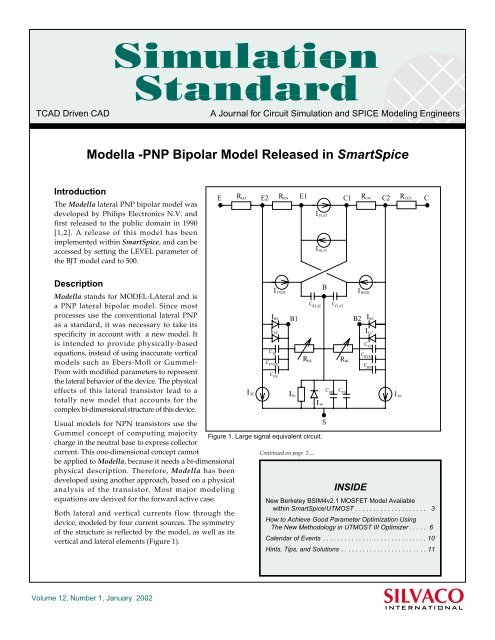
Modella -PNP Bipolar Model Released in SmartSpice - Silvaco

TCAD Driven CAD A Journal for Circuit Simulation and SPICE Modeling Engineers 

Introduction 

Modella -PNP Bipolar Model Released in SmartSpice 

The Modella lateral PNP bipolar model was 

developed by Philips Electronics N.V. and 

first released to the public domain in 1990 

[1,2]. A release of this model has been 

implemented within SmartSpice, and can be 

accessed by setting the LEVEL parameter of 

the BJT model card to 500. 

Description 

Modella stands for MODEL-LAteral and is 

a PNP lateral bipolar model. Since most 

processes use the conventional lateral PNP 

as a standard, it was necessary to take its 

specificity in account with a new model. It 

is intended to provide physically-based 

equations, instead of using inaccurate vertical 

models such as Ebers-Moll or Gummel- 

Poon with modified parameters to represent 

the lateral behavior of the device. The physical 

effects of this lateral transistor lead to a 

totally new model that accounts for the 

complex bi-dimensional structure of this device. 

Usual models for NPN transistors use the 

Gummel concept of computing majority 

charge in the neutral base to express collector 

current. This one-dimensional concept cannot 

be applied to Modella, because it needs a bi-dimensional 

physical description. Therefore, Modella has been 

developed using another approach, based on a physical 

analysis of the transistor. Most major modeling 

equations are derived for the forward active case. 

Both lateral and vertical currents flow through the 

device, modeled by four current sources. The symmetry 

of the structure is reflected by the model, as well as its 

vertical and lateral elements (Figure 1). 

Volume 12, Number 1, January 2002 

E 

REEX E2 REIN E1 

C1 RCIN C2 RCEX C 

I SE 

I FVER 

IRE 

I LE 

CTE 

CFVER 

CFN 

ISE 

R BE 

Continued on page 2.... 

I FLAT 

I RLAT 

I SF 

Figure 1. Large signal equivalent circuit. 

B 

CRLAT CFLAT 

B1 B2 

S 

RBC 

CSD CTS 

I RVER 

INSIDE 

IRC 

I LC 

CTC 

CRVER 

CRN 

New Berkeley BSIM4v2.1 MOSFET Model Available 

within SmartSpice/UTMOST . . . . . . . . . . . . . . . . . . . . 3 

How to Achieve Good Parameter Optimization Using 

The New Methodology in UTMOST III Optimizer . . . . . 6 

Calendar of Events . . . . . . . . . . . . . . . . . . . . . . . . . . . . . 10 

Hints, Tips, and Solutions . . . . . . . . . . . . . . . . . . . . . . . . 11 

I SC 

SILVACO 

INTERNATIONAL

Figure 2. Forward IC vs Vce characteristics. 

Modeled effects are : 

● Temperature (without self-heating) 

● Charge storage 

● Excess phase shift for current and storage charges 

● High-injection 

● Built-in electric field in base region 

● Bias-dependent Early effect 

● Low-level non-ideal base currents 

● Hard and quasi-saturation 

● Weak avalanche 

● Current crowding (DC, AC and 

transient) and conductivity modulation 

for base resistance 

● Hot carrier effects in the collector epilayer 

● Explicit modeling of inactive regions 

● Split base-collector depletion capacitance 

Validation 

In order to validate SmartSpice results, 

values were compared with Philips own 

in-house simulator output. PStar was used 

with test circuits for operating point, DC 

and AC analysis. Outputs for DC simulations 

match between PStar and SmartSpice. 

References 

Examples 

Modella is more complex than Gummel- 

Poon models, because it is composed of 

as much as 6 internal nodes. However 

its symmetry and the nature of the equations 

used lead to convergence with the same 

performance as other models do. 

Typical characteristics for the Modella 

device are presented in Figure 2. 

Modella also accounts for advanced 

effects, such as excess phase. 

The basic Gummel-Poon model is a 

one-pole model, but in fact a bipolar 

device has two poles. This results in 

simulation errors, estimating cutoff 

frequency and gain too high and also 

predicting smaller phase shift. The 

EXPHI parameter of the Modella model 

allows the designer to add the second 

pole phase contribution, expressed in 

radians. Figure 3 presents the small-signal 

gain hFE for an inverter circuit using one 

Modella device. 

[1] ‘Nat. lab Unclassified Report No. 2001/804, Physically 

based compact modeling of lateral PNP transistors.’ F.G. 

O’Hara B.E. 

[2] ‘Nat. lab Unclassified Report No. 6131, A new physical 

compact model for lateral PNP transistors’, F.G. O’Hara, 

J.J.H. van den Biesen, H.C. de Graaff and J.B. Foley. 

Figure 3. Forward current gain vs. frequency and excess-phase 

The Simulation Standard Page 2 January 2002

New Berkeley BSIM4v2.1 MOSFET Model Available Within 

SmartSpice/UTMOST III 

1. Introduction 

So far the BSIM3v3.2 MOSFET model, developed by 

UC-Berkeley, has been considered as the industry 

standard model for deep-submicron CMOS design. It 

was rapidly adopted by IC companies and foundries 

for modeling devices down to 0.25 . However, for 

device scale down to 0.10 , some physical mechanisms 

need to be better characterized. 

BSIM4 model is developed to explicitly address the 

following issues, for which BSIM3v3 was found lacking 

and inaccurate: 

● Modeling of sub-0.13 microns MOSFET devices 

● High-frequency analog and high-speed digital 

CMOS circuit simulation 

● Layout-dependent parasitics model 

UC-Berkeley officially released BSIM4v0.0 for the first 

time on March 24, 2000. Later versions BSIM4v1.0, 

BSIM4v2.0 and BSIM4v2.1 were released on October 11, 

2000, on April, 06 2001 and on October 05, 2001, 

respectively. They account for user’s feedback and 

provide bug fixes over earlier versions. 

This article is intended to give an overview of the 

implementation of BSIM4 within Silvaco products. 

Further details and up-to-date information may be 

found in SmartSpice/UTMOST Modeling Manuals and 

SmartSpice Release Notes. 

Readers interested in obtaining more detail about 

BSIM4 may refer to the Berkeley documentation and 

source code, available for download at: 

http://www-device.eecs.berkeley.edu/~bsim3/bsim4.html 

2. Fundamental Improvements Over 

BSIM3v3.2 

Like BSIM3v3.2, BSIM4 accounts for major physical effects: 

● Short/Narrow channel effects on threshold voltage 

● Non-uniform doping effects 

● Mobility reduction due to vertical field 

● Bulk charge effect 

● Carrier velocity saturation 

● Drain induced barrier lowering (DIBL) 

● Channel length modulation (CLM) 

● Source/Drain parasitic resistances 

● Substrate current induced body effect (SCBE) 

● Quantum mechanic charge thickness model 

● Unified flicker noise model 

Figure 1. BSIM4 DC characteristics. 

BSIM4 has the following major improvements and 

additions over BSIM3v3.2: 

● an accurate new model of the intrinsic input resistance 

for both RF, high-frequency analog and high-speed 

digital applications 

● flexible substrate resistance network for RF modeling 

● a new accurate channel thermal noise model and a 

noise partition model for the induced gate noise 

● a non-quasi-static (NQS) model that is consistent 

with the Rg-based RF model and a consistent AC 

model that accounts for the NQS effect in both 

transconductances and capacitances 

● an accurate gate direct tunneling model 

● a comprehensive and versatile geometry-dependent 

parasitics model for various source/drain 

connections and multi-finger devices 

● improved model for steep vertical retrograde 

doping profiles 

● better model for pocket-implanted devices in Vth, 

bulk charge effect model, and Rout 

● asymmetrical and bias-dependent source/drain 

resistance, either internal or external to the intrinsic 

MOSFET at the user’s discretion 

● acceptance of either the electrical or physical gate 

oxide thickness as the model input at the user’s 

choice in a physically accurate manner 

● the quantum mechanical charge-layer-thickness 

model for both IV and CV 

● a more accurate mobility model for predictive modeling 

January 2002 Page 3 The Simulation Standard

Figure 2. BSIM4 RF/High-Speed model: digital ring oscillator. 

● a gate-induced drain leakage (GIDL) current model, 

available in BSIM for the first time 

● an improved unified flicker (1/f) noise model, which 

is smooth over all bias regions and considers the bulk 

charge effect 

● different diode IV and CV characteristics for source 

and drain junctions 

● junction diode breakdown with or without current 

limiting 

● dielectric constant of the gate dielectric as a model 

parameter 

3. Silvaco Implementation 

The Silvaco implementation of BSIM4 is based on the 

official Berkeley releases. BSIM4 is currently accessible 

within SmartSpice/UTMOST by specifying the model 

selector LEVEL=14. The alias LEVEL=54 is also 

supported for HSpice compatibility. 

The most recent version (BSIM4v2.1) is selected by 

default but older versions may be invoked by specifying 

the model parameter VERSION=0.0, 1.0 or 2.0. In the 

Silvaco implementation, VERSION is a real value and 

not a string, as in the Berkeley code. Consequently, the 

Berkeley syntax VERSION=4.2.1 corresponds to 

VERSION=2.1 in SmartSpice/UTMOST III. A warning 

message is issued when an invalid VERSION number is 

given. It is recommended to systematically use the most 

recent version to benefit from the last Berkeley bug fixes 

and improvements. 

The structure of the original Berkeley code has been 

modified. These changes do not directly involve equations, 

except minor bug fixes in derivatives. So they do not 

affect the accuracy of results but may significantly 

improve convergence. The Silvaco implementation 

offers the best performances regarding speed and 

convergence without any loss of accuracy. 

3.1 Differences Between BSIM4v2.1 and BSIM4v2.0 

BSIM4v2.1 provides bug fixes over its previous version, 

BSIM4v2.0. Most of them were already included in the 

Silvaco implementation of BSIM4v2.0 when UC-Berkeley 

released the new version. Consequently, only the 

changes listed below have been incorporated. They are 

active only if VERSION=2.1 is selected: 

● Gate Induced Source Leakage (GISL) is added to give an 

enormous improvement in simulation convergence. 

Together with GIDL, it makes the gate induced leakage 

component of the substrate current symmetric 

● The warning limits for effective channel length, 

channel width and gate oxide thickness (Leff, 

LeffCV, Weff, WeffCV, Toxe, Toxp and Toxm) are 

substantially decreased to avoid a large number of 

warnings when BSIM4 is used beyond its design 

region. For meaningful results, it is still recommended 

to keep these variables/ parameters within the 

BSIM4 design region. This change is intended only to 

allow users to extend the model beyond this region 

with fewer warnings. 

● The model parameter ACDE is now checked only 

when CAPMOD=3 to avoid useless warning messages 

● The 1/f noise bug fix avoids negative DelClm when 

calculating noise density by turning off the second 

part of the noise density equation 

● In addition, this version adds many variables as output 

such as some of the current components (igs, igd, igb, 

igcs, igcd, isub, igidl, igisl) to ease the model verifications 

3.2 Differences Between BSIM4v2.0 and BSIM4v1.0 

The improvements incorporated into BSIM4v2.0 are 

bug fixes and two new model parameters XL and XW. 

XL and XW are geometry offset parameters due to 

mask/etch effect with default values of 0.0. With these 

changes, the BSIM3 parasitic resistance model file 

becomes a compatible subset of the BSIM4 parasitic 

resistance model. 

In versions 0.0 and 1.0, the value of the intrinsic capacitance 

cbdb of the CAPMOD=0 capacitance model was wrong. 

This has been corrected in version 2.0. 

Also, the computation efficiency is enhanced due to a 

better extraneous node allocation strategy. In version 

2.0, internal drain and source nodes are created only if 

access resistances have non-zero values or if a noise 

analysis is performed with the holistic thermal noise 

model selected (TNOIMOD=1). When extraneous nodes 

collapse, the size of the matrix is reduced, leading to a 

significant gain of speed, especially with large circuits. 


3.3 Differences between BSIM4v1.0 and BSIM4v0.0 

The improvements of BSIM4.1.0 over BSIM4.0.0 are bug 

fixes and an analytical equation for the model parameter 

PIGCD when it is not specified. The relevant changes are: 

● Gate Tunneling Currents: in BSIM4.0.0, PIGCD is set 

to a constant value (1.0) if unspecified. In BSIM4.1.0, 

its default value is given by an analytical equation: 

B ⋅ TOXE 

PIGCD = ----------------------- ⋅ ⎛1– ---------------------- ⎞ 

2 ⎝ 2 ⋅ V ⎠ 

gsteff 

V gsteff 

V dseff 

where B is a constant, set to 7.45669e11 for NMOS or 

to 1.16645e12 for PMOS, and TOXE is a model parameter 

(Electrical gate equivalent oxide thickness). 

● Thermal Noise Charge Based Model (TNOIMOD=0): 

in BSIM4.0.0, the inversion charge Qinv used in the 

thermal noise current formulation depends on the 

effective saturation voltage calculated for the drain 

current equation, which causes a current spike. In 

BSIM4.1.0, this bug has been fixed by replacing the 

original value of Vdsat by a simple expression, 

corresponding to a long-channel saturation voltage: 

V dsat 

V gsteff 

= --------------- 

Abulk ● Parameter checking: in BSIM4.0.0, the maximum 

number of device fingers (NF) is limited to 500. In 

BSIM4.1.0, this limit is removed and if NF is too large 

and makes the effective width (Weff) to be lower 

than or equal to zero, a fatal error will be issued. 

3.4 Silvaco Specific Features 

The following SmartSpice-specific features have been 

added to the original Berkeley implementation, for all 

BSIM4 versions: 

● The BSIM4 code has been optimized to benefit from 

SmartSpice multi-threading capabilities. A gain of 

speed of 30% or more may be observed on 2-processors 

machines, especially when running large circuits 

● The VZERO and BYPASS options are fully supported. 

Specifying VZERO=2 and/or BYPASS=1 on 

.OPTION lines may significantly speed-up computation 

for transient analysis. The original Berkeley BYPASS 

criterion has been modified to ensure accuracy and 

for HSpice compatibility 

● The SmartSpice standard multiplier, useful to put 

several identical transistors in parallel, is supported 

as a BSIM4 instance parameter M. This parameter is 

not equivalent to the instance parameter NF (number 

of fingers) introduced in BSIM4 by Berkeley to 

account for devices in parallel. Please refer to 

Berkeley documentation for further details on this 

new parameter 

● In SmartSpice, it is possible to specify the temperature 

of each device using the standard instance parameters 

TEMP and DTEMP. They are also supported for 

BSIM4 instances. TEMP has the highest priority and 

correspond to the temperature of the device in. If TEMP 

is unspecified and DTEMP is specified, the instance 

temperature is evaluated by adding DTEMP to the 

circuit temperature. If none of these parameters are 

specified the circuit temperature is used, which defaults 

to 27 if unspecified with .OPTION or .TEMP statements 

● The original Berkeley BSIM4 parameter checking 

scheme has been modified to avoid the same warning 

message be issued several times when a parameter is 

out of range. In the Silvaco implementation, instance 

and model parameters are separately tested. As the 

main consequence, each warning message is now 

issued only once 

● The implementation of NQS models has been 

optimized so that related matrix elements are created 

only when TRNQSMOD or ACNQSMOD selector 

are set to 1. That fixes a singular matrix error when 

TRNQSMOD=1 and ACNQSMOD=0 

● The SmartSpice standard conductances GMIN/ 

DCGMIN have been added. They are connected in 

parallel with bulk junction diodes and between internal 

drain and source nodes. They account for the instance 

multiplier (M) and the number of device fingers (NF) 

● The CAPTAB and DCCAP options are supported. 

● The terminal currents and charges can be printed, 

plotted or saved for DC, TRAN and AC analysis using 

the SmartSpice syntax @instance_name[variable_name]. 

The related variable names are listed in Table 1 

Variable name (alias) Definition 

id (cd) Drain terminal current 

cs Source terminal current 

cg Gate terminal current 

cb Bulk terminal current 

*qdrain Intrinsic drain charge 

*qbulk Intrinsic bulk charge 

*qgate Intrinsic gate charge 

*qd Total drain charge 

*qb Total bulk charge 

*qg Total gate charge 

*cqd Total drain capacitance current 

*cqb Total bulk capacitance current 

*cqg Total gate capacitance current 

Table 1. BSIM4 extra output variables added in SmartSpice. 

The variables marked with an asterisk are systematically 

computed after transient and small-signal analysis. For 

DC analysis, they are computed only if DCCAP option 

is turned on. 


How to Achieve Good Parameter Optimization Using The 

New Methodology in UTMOST III Optimizer 

1.Introduction 

What is the goal of optimization? 

The optimization is the task of finding the 

absolute best set of admissible conditions to 

achieve your objective, formulated in 

mathematical terms. The goal of optimization 

is, given a system, to find the setting of it’s 

parameters so that to obtain the optimal 

performance. The performance of the system 

is given by an evaluation function. 

Optimization problems are commonly found 

in a wide range of fields, and it is also of 

central concern to many problems. 

The basic approach in all cases is usually the 

same: User selects or designs a “merit-function” 

that measures the agreement between the 

data and the model with a particular choice 

of parameters. The merit function is generally 

designed so that small values represent close 

agreement. The parameters and the model 

are then adjusted to achieve a minimum in 

the merit function, yielding best-parameters 

set. The adjustment process is thus a problem 

in minimization in many dimensions. The 

computational wish is always the same: do it 

quickly and cheaply. Often the computational effort is 

dominated by the cost of evaluating the merit function 

(and perhaps its partial derivatives). In such cases, the 

wishes are sometimes replaced by a simple goal: 

Evaluate the merit-function as few times as possible. 

Finding a global extremum is, in general, a very difficult 

problem. 

Two standard methods are widely used: 

● find local extrema starting from widely varying 

starting values of the independent variables and then 

pick the most extreme of these 

● perturb a local extremum by taking a finite amplitude 

step away from it, and then see if your method 

returns you a better point, or always to the same one 

(Simulated Annealing)[1] 

Unfortunately, there is no perfect optimization algorithm. 

and the choice of the optimization method is based on 

the following consideration: A selection must be made 

between methods that need only evaluations of the 

“merit-function “to minimize and those that also require 

evaluations of the derivatives of that functions. 

Algorithms using the derivative are somewhat more 

powerful than those using only the function, but not 

always enough so as to compensate for the additional 

calculations of derivatives. 

Successive Line 

Optimization 

(Direction Set) 

No Gradient 

Computation 

Powell s 

Method 

Conjugate Gradient 

Method 

Multidimensional Optimization 

Gradient 

Computation 

Quasi Newton 

Method 

Figure 1. The basic optimization methods. 

General 

(No direction set) 

Downhill Simplex 

Levenberg-Marquardt Simulated Annealing 

Figure 1 describes the two different basic optimization 

methods. One is based on direction-set, the other not. 

The well known Levenberg-Marquardt[2] method is 

associated to the direction-set, the Downhill Simplex 

method and the Simulated annealing are issued from 

the no-direction set way. 

It should take into account that optimization is always a 

question of compromise. The main problem of the 

optimization with spice model is that the cost of an 

evaluation of the merit-function is very high (i.e. it’s 

very long). The Levenberg-Marquardt method 

implemented for many years in UTMOST optimizer 

limit the number of evaluation of the merit-function but 

also computes the derivatives. Now available, the 

Downhill Simplex method does not not compute the 

derivatives. In fact, our goal is to make available 

the Simulated Annealing method in which have 

demonstrated important successes on a variety of global 

optimization problems[3]. 

Reading the following pages you will find an 

explanation of the two optimization methods now 

available in UTMOST. The goal of explanations is to 

give a reader the bases of optimization theory in order 

to perform better optimizations using the two methods. 


2. The Levenberg-Marquardt Method 

2.1 Basic Theory 

The Levenberg-Marquardt method is a standard of 

non-linear least-squares optimization routines[4] 

It defines a merit function and determines the best fit 

parameters by it’s minimization. Given a trial values for 

the parameters the procedure improves the trial 

solution and is repeated until stop decreasing. 

Basically the model to be fitted is y = y(x;a) (2.1) 

where a is the set of parameters and the χ 2 merit function is: 

The basic idea is to take a step down the gradient 

(steepest descent method), that we can write as: 

Where λ is defined as a constant (the step). 

It is conventional to define 

and 

Supposing that the merit function χ 2 (a) is well 

approached by is quadratic form (sufficiently close to the 

minimum) and regarding the equation 2.3 we can write 

This set is solved for the increment δal 

that, added to the current approximation, 

gives the next approximation. 

Given an initial guess for the set of parameters 

a, the Levenberg-Marquardt 

method is as follows: 

(1): compute χ 2 (a) 

N 

χ2( a) 

= yi – y( xi; a) 

∑ ---------------------------σ 

i = 1 i 

anext = acur – λ∇χ2( 2.3) 

α kl 

β k 

(2): Pick a modest value of λ 

1 

-- 

2 

χ2 ∂ 

= -------- ( 2.4) 

∂pk 

(3): Solve the system (2.6) for δa and 

evaluate χ 2 (a +δa) 

= 

2 

1 ∂ 

-- χ2 ( 2.5) 

2∂ak 

∂al 

N 

∑ αklδal l = 1 

= βk ( 2.6) 

(4): If χ 2 (a +δa) ≥χ 2 (a) increase λ by a factor 

f and go back to (3) 

(5): If χ 2 ((a +δa) ≤χ 2 (a)), decrease λ, by a 

factor f, update the trial solution 

a←a+δa and go back to (3) 

( 2.2) 

Also necessary is a condition for stopping and this is 

the goal of the following paragraph that will explain the 

start and stop criteria available in UTMOST. 

2.2. Application 

As you can see in Figure 2 there are many parameters 

that you can change in the UTMOST Optimizer Setup. 

All the optimizer parameters are interrelated. The stop 

criteria that can be specified is present to prevent the 

optimizer from performing unnecessary calculations 

when the convergence is not possible, or that the 

number of calculations needed to reach convergence is 

excessive. The termination code indicates the reason 

why the optimizer stops. If you are not satisfied with a 

optimization result, it will indicate which optimization 

parameters you may change. 

Now, we can explain some of them. 

Marquardt parameter, Marquardt scaling: These 

parameters are the λ (Marquardt parameter) and the 

factor f (Marquardt scaling) that are used in the previous 

chapter. They are the most important parameter the 

methods used. In fact, when an optimization is 

performed the Marquardt parameters decrease or 

increase depending of the result of χ 2 (a +δa). 

If the Marquardt parameters decrease, the optimizer is 

going to converge, this is an iter-pass. On the otherhand, 

if it increases, the optimizer is not on the right track and 

this is an iter-fail.To prevent it from performing unnecessary 

calculations, you can limit the number of maximum 

iter-fail (last row of the stop criteria column) or the 

Marquardt parameter (first row of the stop-criteria 

column). The number of iterations depends on the 

number of Spice parameters the user wants to optimize. 

If n is this number of parameters, a number of n 2 iterations 

is a minimum. 

Figure 2. Optimizer Setup / Status screen (Levenberg-Marquardt) 


In most general cases, when the results of 

the optimization are not convenient, one 

solution is to increase the Marquardt 

parameter value (this value can not be 

higher than 1) and at the same time to 

decrease the Marquardt scaling (that can 

never be lower than 1.2) before starting a 

new optimization. 

3. The Downhill Simplex Method 

3.1 Theory 

The simplex optimization method is easy 

to understand (easier than Levenberg- 

Marquardt) and use. Trials are successively 

performed of a direction of improvement 

until the optimum solution is reached. 

The simplex methods can handle many 

variables with only a few trials, and does 

not require any calculation of derivatives. 

The simplex method is based on an initial 

design of k+1 trials, where k is the number 

of variables. A k+1 geometric figure in a 

k-dimensional space is called a simplex. 

The corners of this figure are called the 

vertices. With two variables the first 

simplex design is based on three trials, for 

three variables it is four trials, etc. This 

number of trials is also the minimum for 

defining a direction of improvement. 

Therefore, it is a timesaving and economical 

way to start an optimization project. After 

the initial trials the simplex process is sequential, with 

the addition and evaluation of one new trial at a time. 

The simplex searches systematically for the best levels 

of the control variables. The optimization process ends 

when the optimization objective is reached or when the 

responses cannot be improved further[5]. 

The algorithm is intended to make is own way downhill 

through the complexity of an N-dimensional topography 

until it encounters a (local, at least) minimum. 

The downhill simplex method must be started not just 

with a single point, but with N+1 points, defining the 

initial simplex. Consider P0 as your starting point, you 

can take the other N points to be 

P i = P 0 + λe i. 

The e i’s are N unit vectors and λ is a constant which is 

the problem’s characteristic length scale. In the 

UTMOST optimization method, this value is not a constant 

but dependent on the initial, the maximum and the minimum 

values of each parameter. Thus, this purely mathematical 

method keeps the physical meaning of the spice model. 

The method takes a series of steps, moving the points of 

the simplex where the function is largest, through the 

opposite face of the simplex to a lower point. These 

BEGINNING 

EXPANSION 

Figure 3. The basic moves of the simplex. 

REFLECTION 

CONTRACTION 

steps are called reflections, and they are constructed to 

conserve the volume of the simplex (maintain in non 

degeneracy). Next the method takes the simplex in 

another direction to make a larger step, and find a 

minimum, it contracts itself in all directions, pulling 

itself in around its lowest (best) point. 

The basic moves are shown in Figure 3. In this figure, it 

shows the possible moves for a step in the downhill 

Simplex method. The simplex, at the beginning of the 

step is a tetrahedron. The simplex, at each step, can be a 

reflection, and expansion or a contraction away from 

the high point. The sequence of such steps will always 

converge to the minimum of the function. 

The basic simplex algorithm consists of a few rules. The 

first rule is to reject the trial with the least favorable 

response value in the current simplex. A new set of 

control variable levels is calculated, by reflection into 

the control variable space opposite the undesirable 

result. This new trial replaces the least favorable trial in 

the simplex. This leads to a new least favorable 

response in the simplex that, in turn, leads to another 

new trial, and so on. At each step you move away from 

the least favorable conditions. 

By that the simplex will move steadily towards more 

favorable conditions. The second rule is never to return 

to control variable levels that have just been rejected. 


Figure 4. Optimizer Setup / Status screen (downhill Simplex). 

The calculated reflection in the control variables can 

also produce a least favorable result. Without this 

second rule the simplex would just oscillate between 

the two control variable levels. 

3.2 Application 

Contrary to the Levenberg-Marquardt method, you can 

see on the Figure 4 that there are only a few parameters 

to control with the downhill simplex method. 

You find the classical error stop criteria (rms, average 

and max error) and the maximum number of function 

evaluation. This stop criteria allows you to limit the 

optimization time. Then the algorithm make is own way 

through the complexity of an N dimensional topography. 

The “merit-function” used in our algorithm is the rms 

(root mean square) error, which is the most commonly used. 

With this method, there is no necessity to define iteration 

fail or iteration pass, the control parameter is the number 

of function evaluations shown in the status column. To 

reduce the optimization time, the best way is to 

decrease the maximum function evaluation in the stop 

criteria column. To perform better optimization, the 

best way is to increase the maximum allowed function 

evaluation, what will also increase the optimization time. 

4. Conclusion 

This article, which will allow users to perform better 

optimization, also presents the new optimization 

method now available in UTMOST. It makes the 

comparison between these two optmization methods, 

which have more advantages than drawbacks. 

References 

The Levenberg-Marquardt method is very 

powerful but is not very useful to use 

when the optimizer is not converged. This 

article, which give the basics of the theory 

also explains what parameters to change 

in the optimizer in order to help it to converge. 

On the otherhand, the Downhill Simplex 

method is very easy to use and preserves 

the physical meaning of the spice 

parameters. As it is based on a very simple 

theory, it is very easy to understand and 

does not have any parameters to tune so 

complicated as in the Levenberg- 

Marquardt method. 

One efficient solution is to use the both 

methods when the first selection does not 

give acceptable results.This is a new 

feature that will allow to perform better 

and faster optimizations. 

The Simulated Annealing method, which 

has demonstrated important successes on 

a variety of global optimization problems will 

be the next step of the UTMOST optimizer. 

This method is based on a modified 

Downhill Simplex method. Simulated 

annealing is a global optimization method 

that distinguishes between different local 

optima. Starting from an initial point, the 

algorithm takes a step and the function is 

evaluated. When minimizing a function, 

any downhill step is accepted and the 

process repeats from this new point. 

[1] S. Kirkpatrick, “Optimization by Simulated Annealing.” 

Science, 220, pp. 671-680, 1983. 

[2] JJ. Moré “Lecture Notes in mathematics”, Numerical 

Analysis, vol 630, pp. 105-116. 

[3] R. Desai, “Combining Simulated Annealing and local 

optimization for efficient global optimization.”, proceeding 

of the 9th Florida AI research symposium, pp. 233-237, 

June 1996. 

[4] Numerical recipes, the art of scientific computing, 1992. 

[5] www.multisimplex.com 


January 

1 

2 

3 

4 

5 

6 

7 

8 

9 

10 

11 

12 

13 

14 

15 

16 

17 

18 

19 

20 

21 

22 

23 

24 

25 

26 

27 

28 

29 

30 ASP DAC - Yokohama,Japan 

31 ASP DAC - Yokohama,Japan 

Calendar of Events 

February 

1 TCAD W/S - Scottsdale, AZ 

EDS Techno Fair-Yokohama 

ASP DAC - Yokohama,Japan 

2 EDS Techno Fair-Yokohama 

ASP DAC - Yokohama,Japan 

3 

4 

5 

6 

7 

8 

9 

10 

11 

12 

13 Int’l Conf. on Microelectronics 

and Interface - Santa Clara, CA 

14 Int’l Conf. on Microelectronics 

and Interface - Santa Clara, CA 

15 Expert W/S - Scottsdale, AZ 

16 

17 

18 

19 

20 

21 TCAD W/S- Chelmsford, MA 

Int’l Forum On Semicon Tech - 

Yokohama - Japan 

22 Int’l Forum On Semicon Tech - 

Yokohama - Japan 

23 

24 

25 Compound Semiconductor 

Outlook - San Mateo, CA 





28 

For more information on any of our workshops, please check our web site at http://www.silvaco.com 

Bulletin Board 

We Have a New Website 

We invite you to check out the new Silvaco website 

fully reconstructed for easier navigation and 

use. We have developed a new products page 

that is much easier to navigate and check up on 

all the latest product releases and updates. You 

can check out news articles and recent events 

pertaining to Silvaco and all of its partners and 

corporate ventures. Silvaco’s web site is still the 

place to come for your generic questions and 

answers to common problems. We hope you 

will visit the new site and feel free to offer any 

suggestions you may have. 

Silvaco Supports University Development 

Silvaco International is proud to provide professional 

grade, full versioned EDA tools to 

Universities nation wide. Universities contribute 

significantly to the development of 

process, device and circuit simulation and are 

funded primarily by the Semiconductor 

Research Corporation (SRC). As an affiliate and 

strong supporter of the SRC, Silvaco provides its 

complete, extensive line of technology at a substantial 

educational discount. The program supports 

the use of semiconductor technology CAD 

by students and faculty, for both education and 

research purposes. The Silvaco University program 

is in part a way of saying “Thank You” for 

all of the academic research that has contributed 

directly to the capabilities of Silvaco Software. 

Default Prove-Up Hearing 

Set for Feb 6, 2002 

Default hearing in Silvaco/Avant case is set for 

Feb. 6, 2002 for two counts, defamation and 

interference. Silvaco is seeking damage of $20M 

plus $6M in interest. The case is a retrial of the 

old Meta case, after the Appeals court remanded 

the case to the Superior Court to fix several 

mistakes from the first trail held in 1997. 

The Simulation Standard, circulation 18,000 Vol. 12, No. 1, January 2002 is copyrighted by Silvaco International. If you, or someone you know wants a subscription 

to this free publication, please call (408) 567-1000 (USA), (44) (1483) 401-800 (UK), (81)(45) 820-3000 (Japan), or your nearest Silvaco distributor. 

Simulation Standard, TCAD Driven CAD, Virtual Wafer Fab, Analog Alliance, Legacy, ATHENA, ATLAS, MERCURY, VICTORY, VYPER, ANALOG EXPRESS, 

RESILIENCE, DISCOVERY, CELEBRITY, Manufacturing Tools, Automation Tools, Interactive Tools, TonyPlot, TonyPlot3D, DeckBuild, DevEdit, DevEdit3D, 

Interpreter, ATHENA Interpreter, ATLAS Interpreter, Circuit Optimizer, MaskViews, PSTATS, SSuprem3, SSuprem4, Elite, Optolith, Flash, Silicides, MC 

Depo/Etch, MC Implant, S-Pisces, Blaze/Blaze3D, Device3D, TFT2D/3D, Ferro, SiGe, SiC, Laser, VCSELS, Quantum2D/3D, Luminous2D/3D, Giga2D/3D, 

MixedMode2D/3D, FastBlaze, FastLargeSignal, FastMixedMode, FastGiga, FastNoise, Mocasim, Spirt, Beacon, Frontier, Clarity, Zenith, Vision, Radiant, 

TwinSim, , UTMOST, UTMOST II, UTMOST III, UTMOST IV, PROMOST, SPAYN, UTMOST IV Measure, UTMOST IV Fit, UTMOST IV Spice Modeling, 

SmartStats, SDDL, SmartSpice, FastSpice, Twister, Blast, MixSim, SmartLib, TestChip, Promost-Rel, RelStats, RelLib, Harm, Ranger, Ranger3D Nomad, QUEST, 

EXACT, CLEVER, STELLAR, HIPEX-net, HIPEX-r, HIPEX-c, HIPEX-rc, HIPEX-crc, EM, Power, IR, SI, Timing, SN, Clock, Scholar, Expert, Savage, Scout, 

Dragon, Maverick, Guardian, Envoy, LISA, ExpertViews and SFLM are trademarks of Silvaco International. 


Mustafa Taner, Applications and Support Engineer 

Q. How can I extract BSIM4 parameters 

using UTMOST III ? 

A. The BSIM4_FI routine in UTMOST III 

MOS module should be used for data collection 

and BSIM4 SPICE model parameter 

extraction. The BSIM4_FI routine features 

are similar to the BSIM3_MG routine. The 

BSIM4_FI routine will collect four types of 

measured data curves from each device: 

1) IDS/VGS @ low VDS bias. 

2) IDS/VDS @ VBS=0V. 

3) IDS/VGS @ High VDS bias. 

4) IDS/VDS @ High VBS bias. 

After the data collection is completed the 

menu item "Measure&extract" in the Fit 

Variables screen should be set to "1". This 

will enable the automatic parameter extraction 

and refinement process. (Figure 1.) 

If the "Measure&extract" flag is set to "1" the extraction 

will start after the measurement is completed or after 

Figure 1. BSIM4_FI routine "Fitting Variables" screen. 

Hints, Tips and Solutions 

Figure 2. Local Optimization Strategy#51 : idvg_large_bsim4 

loading the log file and pressing the "Measure" button 

will start the extraction. The BSIM4_FI routine is very easy 

to use and the routine will extract and refine BSIM4 

parameters with user inputting only few process related 

parameters (TOX, XJ, NCH) in to the fit and opt 

columns of the parameters screen. The extracted parameters 

will be copied into the parameters screen. 

The BSIM4_FI routine is an automatic parameter extraction 

and refinement routine. The simulation and 

local/Global optimization should be performed using 

the ALL_DC routines. The measured data collected with 

BSIM4_FI routine can be shared by any ALL_DC routine. 

After the parameter extraction is completed the quality 

of the fits should be examined by running the SPICE 

simulation against the measured data in ALL_DC 

routine. The further fine tuning of the parameters can 

be achieved by using the Local optimization strategies. 

The local optimization strategies between Satrtegy#51 

and Strategy#60 are developed by Silvaco specifically 

for the BSIM4 model parameter optimization. (Figure 2.) 

Call for Questions 

If you have hints, tips, solutions or questions to contribute, please 

contact our Applications and Support Department 

Phone: (408) 567-1000 Fax: (408) 496-6080 

e-mail: support@silvaco.com 

Hints, Tips and Solutions Archive 

Check our our Web Page to see more details of this example 

plus an archive of previous Hints, Tips, and Solutions 

www.silvaco.com 


Your Investment in Silvaco is 

SOLID as a Rock!! 

While others faltered, Silvaco stood SOLID for 

15 years. Silvaco is NOT for sale and will 

remain fiercely independent. Don’t lose sleep, 

as your investment and 

partnership with Silvaco will only grow. 

SILVACO 

INTERNATIONAL 

USA HEADQUARTERS 

Silvaco International 

4701 Patrick Henry Drive 

Building 2 

Santa Clara, CA 95054 

USA 

Phone: 408-567-1000 

Fax: 408-496-6080 

sales@silvaco.com 

www.silvaco.com 

Products Licensed through Silvaco or e*ECAD 

CONTACTS: 

Silvaco Japan 

jpsales@silvaco.com 

Silvaco Korea 

krsales@silvaco.com 

Silvaco Taiwan 

twsales@silvaco.com 

Silvaco Singapore 

sgsales@silvaco.com 

Silvaco UK 

uksales@silvaco.com 

Silvaco France 

frsales@silvaco.com 

Silvaco Germany 

desales@silvaco.com 

Vendor Partner

Modella -PNP Bipolar Model Released in SmartSpice - Silvaco

You also want an ePaper? Increase the reach of your titles

Delete template?

Save as template?