SPEJBL – THE BIPED WALKING ROBOT Marek Peca, Michal Sojka ...

SPEJBL – THE BIPED WALKING ROBOT
Marek Peca, Michal Sojka, Zdeněk Hanzálek
Department of Control Engineering
Faculty of Electrical Engineering
Czech Technical University in Prague, Czech Republic
Abstract: Construction of a biped walking robot, its hardware, basic software
and control design is presented. Primary goal achieved is a static walking with
non-instantaneous double support phase and fixed trajectory in joint coordinates.
The robot with two legs and no upper body is capable to walk with fixed,
manually created, static trajectory using simple SISO proportional controller, yet
it is extendable to use MIMO controllers, flexible trajectory, and dynamic gait.
Distributed servo motor control over a CAN fieldbus is used. Important points in
construction and kinematics, motor current cascaded control and fieldbus timing
are emphasized. The project is open and full documentation is available.
Keywords: biped robot, feedback control, static gait, cascaded controller, inverse
kinematics
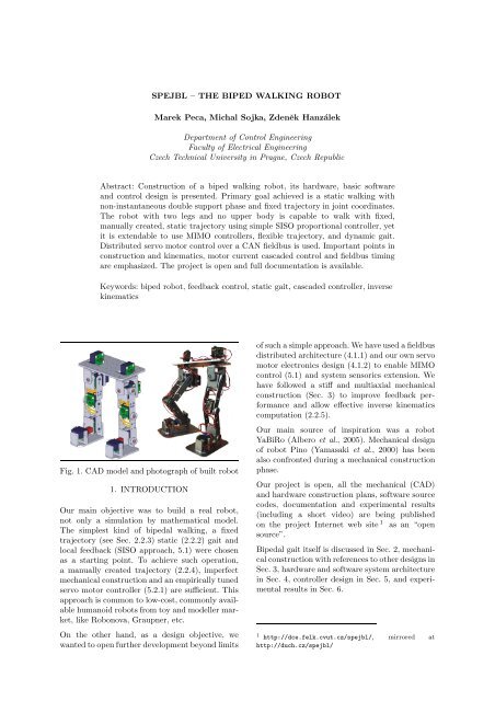
Fig. 1. CAD model and photograph of built robot
1. INTRODUCTION
Our main objective was to build a real robot,
not only a simulation by mathematical model.
The simplest kind of bipedal walking, a fixed
trajectory (see Sec. 2.2.3) static (2.2.2) gait and
local feedback (SISO approach, 5.1) were chosen
as a starting point. To achieve such operation,
a manually created trajectory (2.2.4), imperfect
mechanical construction and an empirically tuned
servo motor controller (5.2.1) are sufficient. This
approach is common to low-cost, commonly available
humanoid robots from toy and modeller market,
like Robonova, Graupner, etc.
On the other hand, as a design objective, we
wanted to open further development beyond limits
of such a simple approach. We have used a fieldbus
distributed architecture (4.1.1) and our own servo
motor electronics design (4.1.2) to enable MIMO
control (5.1) and system sensorics extension. We
have followed a stiff and multiaxial mechanical
construction (Sec. 3) to improve feedback performance
and allow effective inverse kinematics
computation (2.2.5).
Our main source of inspiration was a robot
YaBiRo (Albero et al., 2005). Mechanical design
of robot Pino (Yamasaki et al., 2000) has been
also confronted during a mechanical construction
phase.
Our project is open, all the mechanical (CAD)
and hardware construction plans, software source
codes, documentation and experimental results
(including a short video) are being published
on the project Internet web site 1 as an “open
source”.
Bipedal gait itself is discussed in Sec. 2, mechanical
construction with references to other designs in
Sec. 3, hardware and software system architecture
in Sec. 4, controller design in Sec. 5, and experimental
results in Sec. 6.
1 http://dce.felk.cvut.cz/spejbl/, mirrored at
http://duch.cz/spejbl/

2.1 Definition
2. BIPEDAL GAIT
Bipedal walking is a motion, where at least one of
the feet stays at the floor at any time. The phase,
when a robot stays on only one foot is called
single-support phase, and the other, when the
robot stays on both legs is called double-support
phase. The question is to specify, what does it
mean to stay. For example, we do not accept
gliding as valid element of walking. The foot
should be fixed at the floor by foot-floor friction
forces, eliminating reactional forces, induced by
the motion of the robot.
There are two distinct bipedal gait models: walking
with instantaneous and non-instantaneous
double-support phase. The instantaneous one is a
“limit case” of walking, being close to running
(a motion, where at maximum one of the feet
stays at the floor at any point). It also implies
dynamic gait (see 2.2.2), because the transition
of the centre of gravity (COG) between footprints
can not be done in infinitesimally short time. This
approach is the base idea of many theoretical
biped models (Chevallereau et al., 2004). However,
no real biped using this approach to be able
to walk without external help 2 is known to us at
the moment.
Our concept is to use non-instantaneous double
support phase, although the instantaneous is (at
least theoretically) possible with our robot. The
non-instantaneous one enables static gait (2.2.2)
and will be assumed further.
2.2 Trajectory of gait
2.2.1. Definition Let us define, what we mean
by the trajectory. During the motion of the robot,
each part (rigid body) is moved by forces along
some path in the space, following laws of mechanics.
The robot appears as a serial manipulator with
12 revolute joints (see Sec. 3). It has 12 degrees
of freedom (DOF) in these joints, plus additional
6 DOF, since it is free in the space, ie. it has
no “grounded” link. It means that trajectories
(in world, global sense) of all points of the robot
are fully determined by vector function of dimension
18. However, we work with somewhat
simpler trajectory, which describes only relative
positioning of robot links to each other. It carries
no information about global robot position, so it
stands for 12 DOF. This is the trajectory and it is
2 The robot Rabbit is able to walk, but it requires a
guideline to keep lateral balance (lateral motion has not
been solved intentionally by its team).
defined by displacements (angles) at n = 12 joints,
q(t) : 〈0, tF 〉 → Q, (q1, q2, . . .qn) ∈ Q, where t is
time, tF is walk duration and qk is k-th joint angle,
Q is the space of all possible joint configurations.
It is a trajectory in joint coordinate space Q.
It must be kept in mind, that this 12 DOF trajectory
description is not complete, because actual
position of the robot depends also on impact of
external forces. Eg. robot walking on the floor
is pushed forward by frictional reactional force
of the floor, but if executing the same trajectory
while robot is hanging above the floor, no forward
motion will appear.
This trajectory can be a sufficient description in
the case, when all external forces have known
properties (floor friction, sense of gravity) and
they are homogenous (floor is planar, but can be
inclined). This will be taken in the assumption
in further text, where also a horizontal floor is
mostly assumed. Influence of any differences, as
roughness or inclination of real floor, are regarded
as external disturbance forces.
2.2.2. Static vs. dynamic gait Distinction between
static and dynamic kind of trajectory is a
general issue known from mobile robotics (Choset
et al., 2005). The trajectory can be decomposed
to a path q(s) : 〈0, 1〉 → Q, a continuous function,
giving a curve in Q parametrized by s, and a
time scaling s(t) : 〈0, tF 〉 → 〈0, 1〉, ˙s ≥ 0, so the
trajectory q(t) = q(s(t)).
Given a path q(s), several admissible time scalings
may or may not exist. The time scaling is admissible,
if there exists a function of applied torques
u(t) = (u1, u2, . . . un) satisfying actuator limits
|uk(t)| ≤ ukmax, which produces trajectory q(t).
Assuming the path, a state space of the system
is reduced to scalar position s and velocity ˙s. Actuator
limits together with system dynamics give
constraint on acceleration L(s, ˙s) ≤ ¨s ≤ U(s, ˙s).
A curve in (s, ˙s) satisfying this condition gives
admissible time scaling for given path.
The path is static, if a curve ˙s = 0, s ∈ 〈0, 1〉
gives admissible time scaling. It means, the robot
can stand in any position q(s) without falling,
without any motion. Robot can follow this path
arbitrarily slowly. At each point q(s), the robot
satisfies a condition of statical stability. Trajectory
scaled along this path by s(t) so that ˙s approaches
zero, is called a static trajectory. If a time scaling
with ˙s = 0 is not admissible, but another one with
˙s > 0 is, the result is a dynamic trajectory.
If static or dynamic trajectory together with external
forces form a gait (see 2.1), it is then called
a static gait or dynamic gait, respectively. Further,
a static gait will be assumed, although most of the
rest can be applied for the dynamic gait as well.

trajectory reference
feet
T pelvis reference
COG ref.
COG
+
+
C 2 ∆x, ∆y
flexible trajectory
balancing controller
IK
inverse
kinematic
positional
controller
q(t)
C 1
S
joint angles
COG estimate
Fig. 2. flexible trajectory controller example
2.2.3. Fixed vs. flexible trajectory We distinguish
between fixed and flexible trajectory control.
In fixed trajectory control, q(t) is given and system
is controlled to follow this trajectory. The
operation is reduced to control of dynamic system.
In flexible trajectory control, q(t) is specified partially,
leaving a room for ad hoc trajectory adaptation
to instant situation, by means of disturbance
rejection. This flexibility adds effectively feedback
to the system. If the motors are already enclosed
in positional feedback loop, then the flexible trajectory
generator is an outer feedback loop, forming
together a cascaded controller.
Flexible trajectory control can provide better
rejection of strong disturbances, such as varying
plane inclination or payload consequences on
COG position. Simple example of such a controller
is on Fig. 2. Trajectory is given in carthesian
coordinates of feet and pelvis. Real position of
COG is estimated from sensors (inclinometry, feet
pressure or motor current). It is compared with
reference position of COG and the error is fed back
by a controller to displace pelvis by some ∆x, ∆y
correction. Pelvis then moves aside to balance a
disturbance. To control by displacement in other
than joint coordinates, a real-time computation of
inverse kinematics is needed (see 2.2.5).
The most complicated way of flexible trajectory
adaptation is to change it completely, eg. to place
feet intentionally to prevent falling etc. There
are no implementations of such bipeds known to
us. Implementation of this behaviour for other
walking robots, quadrupeds, has been developped
eg. by (Boston Dynamics, n.d.).
Further, only the fixed trajectory control is assumed.
2.2.4. Trajectory creation The trajectory of
static gait can be divided into two parts: displacement
of COG from above one footprint to another,
and displacement of disengaged foot to another
place. Then, the same but mirrored sequence follows
with feet exchanged.
The trajectory creation can be done manually by
“animation”. Several points q(sk), k = 1 . . .m are
sampled, ie. the robot is “frozen” by feedback at
q(sk) = const., and if this position is statically
stable (see 2.2.2), it can become a point of the
whole trajectory. Then, an interpolation of sampled
points in joint coordinates is done. There
are two factors, which can make the resulting
trajectory flawed:
• sampling is too sparse – points between the
interpolated ones are not guaranteed to satisfy
the condition of static stability;
• speed is too high – validity of static trajectory
is guaranteed only for infinitesimal
speeds and can be broken at higher speed by
robot inertia.
A helpful tool for trajectory creation is an inverse
kinematics solver, see 2.2.5. The inverse kinematics
can be used together with manual animation
to set particular samples, while maintaining user
constraints, eg. feet to lie in planes parallel to
pelvis and to each other, feet to be parallel to
each other, etc.
2.2.5. Inverse kinematics The inverse kinematics
allows to calculate joint angles (q1, q2, . . .qn)
from given relative coordinates between pelvis and
feet. Our robot, when in single-support phase, can
be regarded consisting of two 6 revolute joint (6R)
serial manipulators 3 . Pelvis forms a base link of
these manipulators, and feet form their two end
effectors.
Given a position of the foot relative to pelvis in
carthesian coordinates and some representation
of 3D rotation (eg. Euler angles), the inverse
kinematic solver calculates 6 joint angles to reach
this position. In the case of unconstrained joints
(free 360 ◦ motion), there are up to 2 3 solutions
(2 knee configurations and ambiguity of hip and
ankle angles).
For the 6 joint serial manipulator, containing
3-axes joint, the inverse kinematics can always
be solved analytically (see (Slotine and Asada,
1992)). The implementation is fast and numerically
well-conditioned. The complete set of solutions
is calculated using following floating point
math function calls: 5× atan2 4 , 5× sin and cos,
2× sqrt 5 , 1× acos, 25× multiplication, several
additions or subtractions, no division. One particular
solution is computed, then all 7 remaining
solutions are obtained by additions and subtractions.
In case of position being out of range, the
solution is clamped to straight leg towards the
desired position.
The set of 8 solutions is pruned by application
of joint angle constraints, then an arbitrary one
3 This is exact during single-support phase; however, during
double-support phase, the robot becomes a parallel
manipulator.
4 generalized arctangent, see C language math library
5 square root

solution is chosen. In more advanced approach, a
collision detection could be used to prune the set.
The implemented algorithm works in constant and
reasonably short time, that allows to use it in realtime,
such as in controller feedback, as shown in
Fig. 2.
3. MECHANICAL CONSTRUCTION
Mechanical construction of the biped robot is
inspired by composition and motion capabilities of
human legs (see Sec. 1). The robot is composed of
two legs, each with 6 DOF. No body above a pelvis
is present, nor any additional DOF. Inspiration to
this kind of biped, unable to balance by swinging a
upper body, was taken mainly from robot YABiRo
(Albero et al., 2005).
Each leg is composed of a large, stable foot. It
enables a static gait, maintaining COG above a
footprint of the particular leg or in between them.
It is in contrast to point-like feet of walking multipeds
(quadruped (Ridderström et al., 2000), or
very common hexapods) or exclusively dynamically
walking bipeds (Chevallereau et al., 2004).
Although the large foot is present, a dynamic gait
is also possible.
Each foot is linked to a shank by 2-axis ankle
joint, the shank is linked to a thigh by single
axis knee joint and the thigh is linked to a pelvis
plate, linking both legs, by a 3-axis hip joint. The
multiaxis joints (ankle and hip), are composed of
multiple single axis joints with axes intersecting
in one point and perpendicular to each other. The
multiaxis joints are present to simplify kinematic
description of the robot, in particular to enable
qualitatively simpler inverse kinematics computation
(see 2.2.5). This is not respected in many
modeller biped designs as well as in robot Pino
(Yamasaki et al., 2000).
Each axis is actuated by the same type of servo
motor. The motor is a modeller servo motor
HSR-5995TG by HiTec company, with original
electronics replaced with our own design (see
4.1.2). This servo motor was chosen because of its
compact dimensions and ability to draw a torque
of 2.4 Nm. Modeller servo motor case served as a
base for mechanical construction concept. All axes
are actuated directly by a motor shaft, no rods
have been used, in order to eliminate actuator
springiness. This approach is common to modeller
biped designs and Pino (Yamasaki et al., 2000)
and differs from YaBiRo (Albero et al., 2005),
which uses rods.
Most of the mechanical parts have been designed
to be cut by CNC laser from duraluminium
sheets (AlCu4Mg) of thicknesses 2 mm, 5 mm and
CAN bus
servo
motors
main
control
computer
M
SPEJBL
ARM
SPEJBL
ARM
M
SPEJBL
ARM
time-trigger
Fig. 3. network block diagram
M
SPEJBL
ARM
SPEJBL
ARM
additional
sensors
M
SPEJBL
ARM
SPEJBL
ARM
10 mm. Other parts are: brass distance spacers
with inner M3 thread, bearings DIN 625, special
tiny spindles, ankle blocks and metric screws M3,
M2.5, M2 a M1.6. The overall weight of the robot
is about 2.5 kg.
4.1 Hardware
4. ARCHITECTURE
Each of 12 servo motors is equipped with computer
board “SPEJBL-ARM”, containing 32-bit
microcontroller Philips LPC2119 with ARM CPU
core, and with a CAN (Controller Area Network)
bus interface led out. The board was designed
specifically to fit onto a servo motor case in restricted
space (37 ×28 ×6.5 mm including connectors).
The CPU runs at clock speed up to 60 MHz,
ARM7TDMI core supports 32-bit computation in
integer arithmetics. This gives reasonably strong
computing power for implementation of local motor
controllers. Although it may seem to be an
overkill to use such a strong CPU for each motor,
it must be seen, that commercial price of an 8-bit
microcontroller equipped by CAN was equal to a
price of LPC2119 at the time of design.
4.1.1. Network Servo motor SPEJBL-ARM
boards form 12 nodes on CAN bus network (Fig.
3), representing actuators as well as position sensors
at every DOF. Additional sensors, such as
accelerometers or feet pressure sensors, could be
appended to the system. There is a main control
computer, connected to the CAN bus as well,
gathering measured position data from the servo
motor boards (eventually from other sensors) and
distributing commands to the servo motor boards
for actuation. Currently, the IBM PC is used as
control computer, however it is ready to be replaced
by more handy RISC computer board.
The robot strongly benefits from the usage of a
fieldbus, mainly because of
• the measured analogue values are not led
for a long distances in the neighbourhood of
large actuation pulse currents;
• simple overall cabling, consisting only of 4
wires (2 for power and 2 for CAN bus), allows

great freedom of motion without considerable
collisions between mechanical parts and cabling;
• flexibility in addition of new sensors;
• flexibility in choice of control computer system.
CAN bus has been chosen because of its availability,
reasonable component prices, hardware
support in microcontrollers and great software
support by OCERA LinCAN driver (Píˇsa and
Vacek, 2003).
One additional SPEJBL-ARM board has been
used to serve as a time trigger for the CAN bus
communication, being a bus master for all obeying
nodes, including the control computer. This role
could be played by any other node present, which
has the timing exact enough. As the main control
computer does not provide this functionality, it
has to fulfill much less hard real-time requirements
now. The time-trigger board generates a “tick”
message at the frequency of 250 Hz, which serves
as a global synchronization clock instant to allow
synchronous timing by means of discrete control.
The robot is powered by a cable, because of high
power requirements (it is being powered from
7 V, 10 A supply). Powering from lithium based
accumulator batteries is theoretically possible,
but we have not focused on fully autonomous
operation. According to this, the control computer
is a stationary system and it is connected to the
robot body by a CAN bus cable.
4.1.2. Servo motor electronics Original modeller
servo electronics have not satisfied our needs,
especially for
• lack of suitable interface (CAN or any other
multinode network);
• impossibility of our own motor controller
implementation;
• design flaws regarding current limits (power
transistors caught fire under heavy loads of
motor shaft),
so we have replaced it with our own design. The
electric motor is a DC brushed, coreless one, with
unknown parameters. Operating voltage, according
to HiTec datasheet, ranges between 4.8–7.4 V.
The position (angle) is sensed by potentiometer
(at gear output). The motor is actuated from computer
board by PWM (pulse-width modulation)
switched hard voltage source, and actual current
and position are measured by a 10-bit ADC (analog
to digital converter), contained on LPC2119
chip. Frequency of PWM has been chosen to lie
outside of the human acoustic band, 20 kHz.
Servo motor electronic has been designed with
hardware simplicity in mind, leaving most of the
t k
T
T
T
measured
x 1 x 2 x 3
gathered values
tick msg.
x 12
computation
time
4 ms
Fig. 4. traffic during a CAN bus cycle
t
actuation msgs. k+1
xw1 . . . xw12
T
T
T
actuated
operation up to software. The PWM H-bridge
driver dead time is software defined (4 wire connection).
The sensed current, suffering from high
content of high frequency spurious signals, is filtered
by simple first order RC low pass, followed
by oversampling and averaging.
The current sensing circuitry is a fundamental
part of motor control, as it allows efficient software
defined current limitation using cascaded controller
with software saturation, beside it allows
estimation of external load torque, what may be
used to estimate orientation of gravitation.
4.2 Software
4.2.1. Timing and network SPEJBL-ARM
boards, controlling servo motors, are running
in system-less (without an operating system),
interrupt-driven mode. They execute fast local
control loops, in particular the current control
loop (see 5.2.2), position and current sensing, and
CAN communication with main control computer.
Actually, they do current sampling at 120 kHz,
position sampling and current feedback loop at
20 kHz, what is also the base frequency of PWM.
Currently, the local loop clock runs asynchronously
to the global CAN bus clock (time-trigger). It
causes a sampling jitter, which is considered to be
negligible, as it is in the case of 20 kHz to 250 Hz
ratio less than or equal to 1.25% of longer period.
The main control computer is running Linux 2.6
operating system, in experiments used with no
real-time extensions. Thanks to external timetrigger
and one-period (CAN period, ie. 4 ms) delay
between sampling and actuation, there are relatively
soft real-time requirements imposed on the
main control computer. For jitter-less operation, it
is sufficient if actuation values are computed and
sent between last measurement of k-th period and
time trigger message of (k + 1)-th period arrival,
what is approximately 68% of the CAN period, ie.
about 2.72 ms.
The traffic on the CAN bus during a CAN timetrigger
period is shown on Figure 4. Time-trigger
board sends periodically “tick” messages, containing
8-bit timestamp to allow overrun detection. At
the instant of tick message arrival, servo motor
potentiometers (eventually also other sensors) are
sampled (or recently sensed values are taken).

Gathered values are sent over the CAN bus to the
main control computer, each device naturally uses
its own CAN identifier. Then, the main control
computer determines next values for actuation.
They may or may not depend on gathered values,
depending whether the controller follows MIMO
or SISO approach, respectively (see 5.1). Actuation
values are sent to servo motor computer
boards. To save CAN bus traffic, there are less
actuation messages than motors, as one message
carries values for several motors (now there are 4
16-bit values in 1 actuation message).
The CAN bus is operated at maximum transfer
speed of 1 Mb/s. The period of time-trigger has
been determined from throughput at reasonable
bus load. To estimate maximum network load,
a case of total bit-stuffing ( 6
5
length of stuffable
area) has been considered. Given 1 time-trigger
1-byte message, 12 messages, one from each servo
motor board, 2-byte each (position only sensing),
and 3 actuation messages of 8-bytes, the CAN bus
load at 4 ms time-trigger period is up to 33.2%,
if servo motor sensing messages are extended
to 6-byte (including information about voltage,
cureent and position), the load is up to 44.6%.
SPEJBL-ARM board is equipped with a CAN
bootloader firmware. After the robot is switched
on, its SPEJBL-ARM boards are loaded on-the-fly
by the controller software from the main control
computer.
4.2.2. User software The user software, executed
on the main control computer, is used to
control the robot and to create gait trajectories.
The first version was a simple batch program
with textual input/output, in the present version,
the user software is based on a combination of
graphical user interface (GUI) with text editor of
the trajectory file. The software allows to:
• play a trajectory from text file, using linear
interpolation between points in joint coordinate
space, allowing to change playback
speed and to pause playback;
• record a trajectory or its part in real-time,
allowing fully manual “animation” of the
robot like a marionette, when the motors are
powered-off and only a position is sensed;
• position arbitrary joint by mouse, keyboard
tap or keyboard number input;
• freeze arbitrary subset of joint motors, allowing
to position manually the rest of them.
With SISO control approach (5.1), the user software
acts as a sequencer of trajectory values.
With MIMO approach, the controller is a part of
the user software, operating with base sampling
frequency equal to CAN bus time-trigger period
(see 5.2.2).
C1 M
T
1
a) b)
c)
T C
C 2 M 2
Cn Mn
C 1 M 1
C 2 M 2
Cn Mn
T C
M 1
M 2
Mn
T – trajectory generator
(produces xwk = q k )
C, C 1 . . . Cn – controllers
M 1 . . . Mn – DC motors
Fig. 5. a) SISO, b) MIMO, c) MIMO-SISO cascaded
The software will be integrated with inverse kinematic
solver (see 2.2.5) and OpenGL visualization,
allowing smooth transition between positioning
in joint and world coordinates.
5. CONTROL DESIGN
The robot is regarded as a mechanical system
consisting of rigid bodies, springiness of the motor
shafts is neglected. According to Lagrange formulation,
a state vector contains 12 (angle) positions
and 12 (angular) velocities, giving the system of
order 24. The input forces to the system are internal:
12 motor torques and joint friction, and
external: floor reaction, friction, gravitation and
disturbances. The output is 12 joint positions xk,
desired to approach reference trajectory xwk = qk.
5.1 SISO vs. MIMO approach
There are two base concepts of a biped trajectory
controller. The simpler one is composed by multiple
SISO (single-input, single-output) controllers,
one controller per one servo motor. Each motor
is controlled independently by its dedicated controller
(Fig. 5a). A disadvantage of this approach
is, that mutual dynamics between robot parts is
ignored, controllers are unable to “cooperate”.
The advantage is a simplicity.
In SISO approach, each controller can be tuned
separately, depending on its position (joint, where
it does act), also the online parameter change
could be performed during distinct gait phases.
However, for the maximum simplicity, all controllers
can be identical, robust enough to achieve
stability for all joints and gait phases, at the cost
of a lower control performance. Typically, a PID
or a cascaded PID controller is a suitable choice
for this kind of controller.
On the other hand, a single MIMO (multipleinput,
multiple-output) controller can be em-

xw
z −1
250 Hz
ZOH +
−
C
u
1 kHz
S
Fig. 6. block diagram of type P controller
ployed instead (Fig. 5b). Command signal is a
vector, whose components are fed to all motors.
All measured positions are returned to the controller
as a measured system output, and could be
accompanied by measurements from other sensors
(gravitational inclinometry, feet pressure sensors)
to refine position estimation in MIMO controller.
The command signal can in theory set directly
the PWM (voltage) value to motor. In practice, at
least a current controller should enclose the motor
to protect it against overcurrent destruction,
forming together a MIMO-SISO cascaded control
system (Fig. 5c).
The advantage of the MIMO approach is that
it can reflect interacting system dynamics and
that it allows a sensor fusion of servo motor
potentiometers combined with other sensors. The
controllers suitable for this design are eg. LQG,
general observer-feedback controller, designed eg.
by pole-placement, maybe also a native nonlinear
controller (designed eg. by exact linearization).
5.2 Controllers implemented
5.2.1. SISO, simple type P The first controller
used in our robot was the simplest type P (proportional
only) controller, taking position as a
system output and voltage (PWM) as a command
variable, see Fig. 6. Plant S, consisting of a DC
motor linked to rigid mass, with output position
(angle) x controlled by C outputting voltage u.
Sample rate transition is done by zero-order hold
(ZOH), inherent one-sample delay of CAN bus
traffic z −1 lies outside of the loop.
K
DC motor transfer function S(s) = s(1+sTm) is
assumed, time constant has been identified with
no mass linked to as Tm = 0.014 s. Feedback loop
is closed locally in software of the servo motor
control board. Sampling frequency of this loop
has been chosen to be fs1 = 1 kHz. The CAN
bus is used only to deliver reference value xw
to the controller and its sampling frequency is
fs2 = 250 Hz.
5.2.2. SISO, cascaded PID-PI The second controller
has been designed to enable current limitation
in servo motors and to close positional
feedback through the CAN bus, allowing SISO
to be then replaced by MIMO in control design
(leaving inner current controller loops in all servo
x
z
+
ZOH C1 S1 S2 −
−1
xw + iw
C2 u i x
−
↓D
MA
250 Hz 20 kHz
Fig. 7. block diagram of cascaded PID-PI controller
motors). Cascaded controller topology has been
used, see Fig. 7.
DC motor model is split into two parts: S1,
producing winding current i as a response to drive
voltage (PWM) u, and S2, producing position
(angle) x as a response to current i. Measured
electric admittance of the DC motor is fairly close
to DC conductance up to order of 105 Hz, so
the electric dynamics is neglected and subsystem
modelled statically as S1(s) = K1. The motion
K2
equation of the motor gives S2(s) = s(1+sTm) .
The inner loop contains current controller C1 with
limitation, implemented as a software saturation
imposed on the reference current variable iw (iw
is clamped to not exceed maximum allowable absolute
value of the current). Controller of type PI
has been used. Integral action has been employed
to assure rejection of constant load disturbance.
Derivative action is not present, because dynamics
of the inner loop is much faster than of the
mechanical part of the system.
C2 is a positional controller with current iw as
a command variable. A full PID controller has
been used. Integral action allows to follow a ramp
with zero steady-state error and to reject constant
load disturbance. Inner current loop runs at the
sampling frequency of fs1 = 20 kHz, synchronous
with PWM, outer loop is closed through a CAN
bus at the sampling frequency of fs2 = 250 Hz.
Inherent one-sample delay of CAN bus z −1 lies
inside of the outer loop. Sample rate transition is
done by ZOH and decimation ↓D. Measured value
x is filtered by moving average filter (MA) to suppress
a noise. Both elements, z −1 and MA, have
significant impact on phase response of controlled
system.
6. EXPERIMENT
6.1 Experiment with SISO, type P controller
Reference and measured trajectories of the first
walk, controlled by SISO type P controller, are on
Fig. 8, detailed plot of left lateral hip axis joint is
on Fig. 9. At some joints, especially lateral ankle
and hip joints, relatively large steady state error
is observed. It is caused by strong gravitation load
disturbance.

ight̷hip
transversal
right̷hip
lateral
right̷hip
sagittal
right̷knee
(sagittal)
right̷ankle
sagittal
ankle
lateral
left̷hip
transversal
left̷hip
lateral
left̷hip
sagittal
left̷knee
(sagittal)
left̷ankle
sagittal
left̷ankle
lateral
0
1
2
3
4
5 6
t̷[s]
Fig. 8. trajectory of one step
x L5 ̷[deg.]
̷15
̷0
-15
-30
-45
0
1
2
3
4
5 6
t̷[s]
Fig. 9. detailed trajectory of left lateral hip joint
during one step
The steady state error together with mechanical
hysteresis of hip joint in the first version of robot
mechanics made trajectory creation difficult. If a
measured position was to be “frozen”, an error in
actual configuration occured. The hysteresis was
a severe fault, and has been corrected by bearing
redesign. The steady state error of plain P type
controller is eliminated by use of integral action.
Under inadvisable conditions (heavy loads, mechanical
short circuit), the hard voltage drive of
the motors caused an overcurrent, followed sometimes
by burn down of power H-bridge stage. This
led us to implementation of the current limiting
controller.
7. CONCLUSION
This paper presented a fully operational walking
biped robot built in our laboratory. It is designed
as an open experimental system to test various
controllers. As a first step, it has been experimentally
proven, that a 12 DOF walk is possible using
simple proportional controller and fixed, manually
created trajectory. The ultimate goal is to develop
more advanced MIMO controllers, and automatic
and flexible trajectory generation.
7
7
8
8
9
9
x w
x
x wx
10
10
11
11
We have been convinced of the importance of a
good mechanical construction. The stiffness and
minimal hysteresis are crucial to a successful use
of feedback. Construction of complicated multiaxis
joints allowed us to compute the inverse kinematics
effectively. Use of current limiting inner
loop controller has been considered to be necessary.
Our current and future work includes: automatic
trajectory generation based on COG computation,
Lagrangian model identification, MIMO controller
design, addition of sensors of pressure or
inclination, flexible trajectory control.
The project is open, future collaboration on the
control design and experiments is welcome. This
work was supported by Academy of Science of
the Czech Republic under Project 1ET400750406
and by the Ministry of Industry and Trade under
Project RPN/57/06.
REFERENCES
Albero, M., F. Blanes, G. Benet, P. Perez, J. E.
Simo and J. Coronel (2005). Distributed
real time architecture for small biped robot
YaBiRO. In: IEEE Intl. Symposium on Computational
Intelligence in Robotics and Automation.
Boston Dynamics, Inc. (n.d.). The ”BigDog”
robot, http://www.bdi.com/content/
sec.php?section=bigdog.
Chevallereau, C., E. R. Westervelt and J. W. Grizzle
(2004). Asymptotic stabilization of a fivelink,
four-actuator, planar bipedal runner. In:
43th IEEE Conference on Decision and Control.
Paradise Island, Bahamas.
Choset, H., K. M. Lynch, S. Hutchinson, G. Kantor,
W. Burgard, L. E. Kavraki and S. Thrun
(2005). Principles of robot motion: theory,
algorithms, and implementation. MIT Press.
London, England.
Píˇsa, P. and F. Vacek (2003). Open source components
for the CAN bus. In: Proceedings of
the 5th Real-Time Linux Workshop. Valencia,
Spain.
Ridderström, C., J. Ingvast, F. Hardarson,
M. Gudmundsson, M. Hellgren, J. Wikander,
T. Wadden and H. Rehbinder (2000). The basic
design on the quadruped robot Warp1.
In: Intl. Conference on Climbing and Walking
Robots. Madrid, Spain.
Slotine, Jean-Jacques E. and H. Asada (1992).
Robot Analysis and Control. John Wiley &
Sons. New York, USA.
Yamasaki, F., T. Miyashita, T. Matsui and H. Kitano
(2000). Pino the humanoid: A basic
architecture. In: 4th Intl. Workshop on
RoboCup. Melbourne, Australia.