Feature-guided Image Stippling - Postech Computer Graphics ...

Eurographics Symposium on Rendering 2008 

Steve Marschner and Michael Wimmer 

(Guest Editors) 

Feature-guided Image Stippling 

Dongyeon Kim 1 , Minjung Son 1 , Yunjin Lee 2 , Henry Kang 3 , and Seungyong Lee 1 

1 POSTECH, Korea 2 Ajou University, Korea 3 University of Missouri, St. Louis, USA 

Volume 27 (2008), Number 4 

Abstract 

This paper presents an automatic method for producing stipple renderings from photographs, following the style 

of professional hedcut illustrations. For effective depiction of image features, we introduce a novel dot placement 

algorithm which adapts stipple dots to the local shapes. The core idea is to guide the dot placement along ‘feature 

flow’ extracted from the feature lines, resulting in a dot distribution that conforms to feature shapes. The sizes of 

dots are adaptively determined from the input image for proper tone representation. Experimental results show 

that such feature-guided stippling leads to the production of stylistic and feature-emphasizing dot illustrations. 

Categories and Subject Descriptors (according to ACM CCS): I.3.3 [Picture/Image Generation]: Display algorithms; 

I.3.4 [Graphics Utilities]: Paint systems 

1. Introduction 

Describing a scene with a set of points has been an important 

and challenging issue in many areas of computer graphics, 

such as non-photorealistic rendering (NPR), visualization, 

and digital halftoning. In this paper, we focus on pointbased 

scene stylization, in particular, the problem of generating 

stylistic stipple illustrations from photographs. 

Many of the previous stippling algorithms were developed 

and presented in the context of sampling. Assisted by 

carefully designed dot spacing schemes, they produce a dot 

distribution with reduced visual artifacts, such as aliasing. 

When used for image-based stippling, these algorithms fill 

the image with well-spaced dots that properly describe the 

local tone. However, they do not in general take into account 

the shape or directionality of image features. 

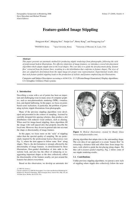
In this paper, we focus more on the ‘style’ of stippling 

rather than the spectral quality of sampling. We are particularly 

inspired by the professional hedcut illustrations (see 

Fig. 1), where the dots appear to follow some ‘flow’ along 

shapes. That is, the dot formation is strongly affected by the 

directionality of image features. As demonstrated by these 

illustrations, flow-guided distribution of dots adds to the 

stylistic look, and also has the effect of enhancing or exaggerating 

important shapes as the dots collectively reflect 

the directionality of the features nearby, not just around the 

features but almost everywhere. 

Based on this observation, we develop an automatic dot 

c○ 2008 The Author(s) 

Journal compilation c○ 2008 The Eurographics Association and Blackwell Publishing Ltd. 

Published by Blackwell Publishing, 9600 Garsington Road, Oxford OX4 2DQ, UK and 

350 Main Street, Malden, MA 02148, USA. 

Figure 1: Hedcut illustrations created by Randy Glass 

(www.randyglassstudio.com) 

placing algorithm that adapts dots to the surrounding shape. 

The core idea of our approach is to create ‘feature flow’ by 

extracting a distance field and offset lines from image features, 

with which to guide the dot placing along shapes. We 

thus call it feature-guided stippling. Fig. 2 shows some of 

our stipple rendering results. 

1.1. Contributions 

Unlike previous stippling algorithms, we pursue a new style 

of stippling where stipple dots collectively follow the near

D. Kim, M. Son, Y. Lee, H. Kang, & S. Lee / Feature-guided Image Stippling 

est image feature direction. To the best of our knowledge, the 

concept of ‘directional stippling’ is new in the field and has 

not been attempted. Imitating the visual quality of hedcut illustrations 

is particularly challenging as it demands artistic 

intuition and finesse in creating flow as well as in arranging 

dots. As a computerized solution, we propose a constrained 

Lloyd algorithm that uses a set of lines offset from the feature 

lines. We also provide adaptive control of the influence 

from offset lines to the Voronoi cells with respect to the distances 

from the feature lines. In addition, our method allows 

for an intuitive control of rendering style with just a few parameters. 

2. Related Work 

2.1. Digital image halftoning 

Image halftoning refers to a technique that approximates the 

original image with a limited number of intensity levels, typically 

black and white [FS76,Ost01,PQW ∗ 08]. Since an output 

of halftoning is often a collection of black dots (pixels) 

on a white image, it may be viewed as a kind of stipple 

illustration. While halftoning is a visual approximation 

technique, stippling is more of an artform. In general, more 

freedom is given to stippling in controlling the size, density, 

shape, style, orientation, and intensity of the dots. Deussen 

et al. [DHVOS00] also pointed out that additional lines (such 

as feature lines) are often used in stippling to allow dots to 

interact with those lines. 

2.2. Stippling 

Salisbury et al. [SWHS97] presented a pen-and-ink illustration 

technique, which is capable of producing stipple illustrations 

when pen strokes are replaced with dots. They 

use a difference image algorithm to produce a roughly 

even dot distribution in local neighborhood. Deussen et 

Figure 2: Stipple illustrations created by our method 

(a) Non-directional (b) Directional (our method) 

Figure 3: Non-directional vs. Directional dot placing. (a) 

produced by the method of [Kopf et al. 2006]. (b) our 

method. In both figures, the same line drawing is superimposed 

onto the output of stippling. 

al. [DHVOS00] presented a stipple drawing method based 

on Lloyd algorithm (i.e., construction of a centroidal 

Voronoi diagram) for more rigorous dot spacing, resulting 

in an exquisite illustration. Secord [Sec02] later modified 

this algorithm to produce a weighted centroidal Voronoi diagram 

that protects image features better than the constantweighted 

version. 

Stippling algorithms often rely on sophisticated sampling 

principles. In particular, many of them reduce aliasing artifacts 

by seeking a sampling property known as blue noise 

spectral characteristics. A dart throwing algorithm [Coo86] 

is a simple method to generate such point sets. Cohen et 

al. [CSHD03] presented a Wang-tile-based method to produce 

blue noise dot distribution, assisted by Lloyd relaxation. 

Kopf et al. [KCODL06] later proposed a recursive 

Wang tiling method for dynamic control of the point set den- 


Journal compilation c○ 2008 The Eurographics Association and Blackwell Publishing Ltd.


Distance field 

Offset lines 

FEATURE FLOW 

CONSTRUCTION 

Initial dots 

Optimized dots 

DOT 

OPTIMIZATION 

Rendered dots 

Input image Output image 

Line map 

RENDERING 

Figure 4: Process overview: For better visualization, in the dot optimization step, the dots in the background are not shown. 

sity. Ostromoukhov et al. [ODJ04] introduced a fast blue 

noise sampling algorithm based on Penrose tiling, which 

was later improved by Ostromoukhov [Ost07] using rectifiable 

polyominoes for better spectral quality. These latter 

algorithms [KCODL06,ODJ04,Ost07] are all very fast, producing 

millions of dots per second, as the Lloyd relaxation 

step is preprocessed. Mould [Mou07] recently presented a 

stippling algorithm based on graph search (instead of Lloyd 

relaxation) for improved protection of image features such 

as edges. 

While all of these cited algorithms are capable of producing 

high-quality stipple illustrations, they do not provide an 

important characteristic we are looking for – the collective 

dot alignment with local shapes. That is, they basically take 

into account the tone but not the shape of the surrounding region, 

and thus the resulting dots do not by themselves reveal 

any sense of directedness. This is illustrated in Fig. 3. While 

some algorithms [DHVOS00, Sec02, Mou07] do protect image 

features, they do not go as far as guiding all of the dots 

along some smooth feature flow. 

2.3. Tile mosaics 

Hausner [Hau01] showed that the centroidal Voronoi diagram, 

when computed with Manhattan distance metric, can 

constrain rectangular tiles to align with some user-defined 

feature lines and the associated direction field. While our 

problem is similar to that of tile mosaics, distributing dots as 

in hedcut illustrations requires much more rigor and finesse 

as it calls for strict alignment of dots almost everywhere (see 

Fig. 1). 

We thus build on Hausner’s constrained Lloyd algorithm 

and adapt it to handle the feature-guided distribution of circular 

dots, rather than rectangular tiles. In particular, we incorporate 

a new set of constraints based on offset lines, to 



enable tight alignment of dots which directly improves the 

quality of the resulting illustration. 

2.4. Engraving 

Ostromoukhov [Ost99] addressed the problem of featuredriven 

tone representation in the context of facial line engraving. 

While his system generates a beautiful set of engraving 

lines flowing across the facial surface, it requires 

considerable user interaction as the line directions are determined 

by the user’s interpretation of the facial structure. 

We aim to build an automatic and general method that can 

handle images of arbitrary scenes. 

3. Overall Process 

Fig. 4 illustrates the overview of our stippling scheme. We 

first process the input image to get it ready for the main stippling 

procedure. This initial process includes tone map and 

line map creation. The tone map controls the tone-related dot 

attribute, i.e., the size, while the line map dictates the shaperelated 

dot attribute, i.e., the location. In the next step, we 

form a feature flow by extracting a distance field and a set 

of offset lines from the line map. The system then optimizes 

the regularly sampled initial dots using a constrained Lloyd 

algorithm, for which we use offset lines as constraints so that 

the dots can closely follow the feature flow. Upon computing 

the sizes of dots, the system produces the target illustration 

by rendering dots together with the feature lines. 

4. Preprocessing 

4.1. Tone map construction 

We use a grayscale image I(x) as input, where x = (x,y) denotes 

an image pixel. In case I is too dark or of low contrast,


we perform brightness adjustment and/or contrast stretching 

on I. The resulting image is denoted T (x), which we call 

a tone map. We let T (x) range in [0,1], where 0 represents 

black. The tone map is used to control the tone-related attribute 

of dots, which is the size (see Sec. 7). 

4.2. Line map construction 

From T (x), we derive a set of feature lines that will be used 

to guide stippling. For feature line detection, we employ the 

line drawing method presented by Kang et al. [KLC07]. The 

method uses the flow-based difference of Gaussians (FDoG) 

filter steered by the edge tangent flow (ETF) field, and produces 

stylistic and coherent lines from important features 

while suppressing noise. Fig. 5 shows an example input and 

the resulting line drawing image. The resulting black-andwhite 

line map is denoted by L(x) ∈ {0,1}, where 0 (black) 

represents line. 

(a) Input (b) Line map 

Figure 5: Line map construction 

5. Feature Flow Construction 

By a ‘feature flow’, we mean a smoothly varying vector field 

that describes the direction of the nearest feature for each 

pixel. To obtain a feature flow, we perform distance transform 

from the feature lines. A distance field can be viewed as 

a vector field, where each pixel x is associated with a vector 

pointing to the neighboring pixel that has the same distance 

value. This vector represents the nearest feature direction at 

x. The constructed distance field is then smoothed to reduce 

potential visual artifacts in the rendering result. Finally, we 

extract offset lines from the smoothed distance field. 

5.1. Distance transform 

The line map L(x) may contain some isolated black pixels 

due to image noise. We first remove these noise pixels by 

binary morphological opening on L(x) with a circular structuring 

element of radius 3. 

We then apply jump flooding method [RT06] to construct 

a distance field, denoted by D(x), using the black pixels in 

L(x) as seeds (zero distance). Jump flooding is so named as 

it propagates information in the manner of ‘jumping’ from 

pixel to pixel. Let k denote the jump (step) size. In each 

round of jumping, each pixel x = (x,y) inspects nine pixels 

located at (x+i,y+ j) where i, j ∈ {−k,0,k}, and computes 

distances to their associated seeds. The minimum of these 

distances and the corresponding seed are recorded at D(x). 

This jumping is repeated by halving k in each round. Therefore, 

the distance field is completed after logn rounds for an 

image of size n × n. 

We can use other distance transform algorithms 

[FCTB08] for constructing a distance field from feature 

lines. However, since jump flooding operates locally on each 

pixel, it can be dramatically accelerated when implemented 

on a GPU. More importantly, it provides constant time 

complexity, regardless of the number of seeds. For more 

details of the algorithm, readers are referred to [RT06]. 

Fig. 6b shows a distance field computed by jump flooding. 

(a) Input (b) Distance field (c) Offset lines 

Figure 6: Feature flow construction. In (c), the feature lines 

and smoothed offset lines are drawn in black. 

5.2. Distance field smoothing 

When we obtain an offset line image, a crude distance field 

may result in some undesirable visual artifacts such as wobbly 

lines and sharp corners. It is desirable to reduce such 

artifacts as they may become noticeable in the final rendering 

and hence divert the viewer’s attention. We resolve this 

by obtaining offset lines from the low-pass filtered distance 

field. We use the Gaussian filter of kernel size σ (by default, 

σ = 5). The filtered distance field results in smooth offset 

lines with rounded corners (see Fig. 6c), which could help 

reduce visual artifacts in the final stipple illustrations. 

5.3. Offset line extraction 

Given the smoothed distance field, the offset lines are extracted 

by regularly sampling the distance values. Let m denote 

the sampling interval, and l denote the desired width of 

each offset line. To create an offset line image, we mark a 

pixel x if its distance D(x) satisfies i · m ≤ D(x) 

where i is a non-negative integer. Typical values we use are 

m = 6 and l = 4. As shown in Fig. 6c, the collection of offset 

lines clearly describe the feature flow. Such an offset line 

image is used to line up dots within the set of white lanes, 

called offset lanes. The width of each offset lane, denoted by 

o, is obtained as o = m − l. The use of a smaller o results in 

stricter alignment of dots. 



6. Dot Optimization 


Given the offset lines and feature lines, the system now performs 

actual stippling. We first scatter the initial distribution 

of dots, which is then optimized by the Lloyd relaxation. 

Here we use the offset lines to constrain the Lloyd algorithm 

so that the dots strictly follow the feature flow. 

6.1. Dot initialization 

For fast initialization, we regularly sample the image pixels 

in both x and y directions, except on the feature lines 

where no dots are sampled. The sampling interval, denoted 

by r, is automatically computed using m, the distance between 

the adjacent offset lane centers. To fill the entire image, 

except on the feature lines, with a disjoint set of circles 

of diameter m, we set r = m. By matching the sampling interval 

of dots with that of the offset lanes, we can force the 

distances between the adjacent dots to be roughly identical 

in both intra-lane and inter-lane directions, after relaxation. 

The intra-lane direction corresponds to the feature flow direction, 

and the inter-lane direction refers to its perpendicular 

direction. 

6.2. Constrained Lloyd relaxation 

The initial dots then go through the Lloyd relaxation. That 

is, we iterate the process of (1) constructing a Voronoi diagram 

from dots, (2) moving dots to the updated centroids of 

Voronoi cells. 

6.2.1. Constructing a Voronoi diagram 

For constructing a Voronoi diagram, we again use the jump 

flooding algorithm, this time however with respect to the 

dots as seeds. Note the jump flooding algorithm creates not 

only a distance field but also a Voronoi diagram as it records 

which seed is associated with each pixel. As opposed to the 

conventional polygon-based z-buffering algorithm for constructing 

a Voronoi diagram [HKL ∗ 99], jump flooding provides 

constant time complexity regardless of the number of 

dots. We use the Euclidean distance in creating a Voronoi 

diagram with jump flooding. 

6.2.2. Updating centroids 

The centroid c of a Voronoi cell is computed as follows; 

c = 1 

ρ ∑ i 

wi · xi 

where xi denotes the i-th pixel in the cell, wi associated 

weight, and ρ = ∑i wi a weight normalization term. In the 

basic Lloyd algorithm, wi = 1 for all pixels in the cell. 

In our approach, we use offset lines as constraints so as the 

Voronoi cells to line up with those lines (see Fig. 7). For this, 

we modify Hausner’s idea which was used to push rectangular 

tiles away from the feature lines [Hau01]. When a part of 



(1) 

a Voronoi cell is occluded by an offset line, we remove the 

part in computing the updated centroid of the cell. We can 

easily achieve this by setting wi = 0 in Eq. 1 for all the pixels 

within offset lines. If a Voronoi cell is divided by an offset 

line, the resulting non-occluded pieces may occupy different 

offset lanes. Among the pieces, we select the closest one 

to the previous centroid, then compute the new centroid of 

the cell using this selected piece only. However, this case of 

multiple pieces rarely happens in our setting where the dot 

sampling interval r is the same as the offset line sampling 

interval m. 

(a) (b) (c) 

Figure 7: Voronoi cell alignment using offset lines. Constrained 

Lloyd relaxation pushes each cell’s centroid towards 

the center of its associated offset lane, as shown from 

(a) to (c). For visualization purpose, the offset lines are 

drawn thinner than they actually are. 

This strategy has the effect of moving a Voronoi cell centroid 

towards the center of an offset lane. It also ensures that 

once the centroid moves into a particular offset lane, it stays 

in there. Fig. 8 shows the evolution of an entire Voronoi diagram, 

constrained by the offset lines. Note our offset-linebased 

constraint is stronger than Hausner’s in that it ‘strictly’ 

aligns dots with the nearest feature lines (see Fig. 9 for comparison). 

(a) Input (b) Initial configuration (c) Final configuration 

Figure 8: Evolution of a dot distribution. See how the constrained 

Lloyd algorithm re-organizes the initial dots to follow 

the feature flow. 

We provide an additional control to prevent the dots from 

looking ‘too structured’ especially in the middle of an area 

away from the feature lines. We accomplish this by weakening 

the offset-line constraints as the distance from the feature 

lines increases (see Fig. 10). We compute the centroids 

c1 and c2 with and without the offset line constraints, respectively, 

and interpolate them using the distance from feature 

lines. That is, the updated centroid c is determined by 

c = (1 − α) · c1 + α · c2 

(2)

(a) Hausner’s method (b) Our method 


Figure 9: Comparison with Hausner’s method. Our method 

produces a more strictly aligned dot distribution. 

where α = min{D(c0)/Dw,1}. Dw is the minimum distance 

for which the offset-line constraints have no effects (by default, 

Dw = 100). c0 is the current centroid before update. 

(a) No control (b) Control with distance 

Figure 10: Adaptive control of the influence of offset lines 

Besides the offset lines, we use the feature lines (i.e., 

black lines in L(x)) as constraints. In addition, with the extraction 

process in Sec. 5.3, offset lines include the areas enclosing 

feature lines, where D(x) < l. As a result, the dots 

do not directly overlap with the feature lines and thus we can 

protect the features better. 

6.2.3. Iteration 

We typically iterate the Lloyd algorithm t1 times without 

offset-line constraints, then t2 times by alternating Lloyd algorithm 

with/without constraints (by default t1 = 5,t2 = 20). 

The first t1 iterations is for spreading the initial set of dots 

over the image. The reason for toggling the constraints on 

and off afterwards is similar; to avoid clustering and spread 

the dots more evenly across the image while following the 

feature flow. 

7. Rendering 

Once the locations of dots have been finalized, they are rendered 

as black circles, together with the feature lines. The 

dot size is inversely proportional to T (x), meaning small 

dots are placed on a bright area, and big dots on a dark area. 

The dot size s at pixel x is thus a function of T (x), which we 

define as follows; 

s(x) = smax · (1 − T (x)) 1/γ 

where smax is the maximum possible dot size and depends 

on the rendered image size. γ is used to incorporate gamma 

(3) 

correction for tone control. With a larger value of γ, we can 

have higher contrast of tones in the stippled image (γ = 1.3 

by default). In the brightest area, where s(x) is less than a 

small threshold, no dot is drawn. 

To improve the quality for printing, it is often a good idea 

to use a set of huge dots rendered in an expanded image 

space and scale down the rendered image. We typically render 

on an image which is six times bigger than the input in 

both horizontal and vertical directions. 

8. Results 

In Fig. 11, we show that a variety of results can be obtained 

from an input image using different values of parameters 

m (offset lane sampling interval) and γ (gamma correction 

value). For the offset line width, we used l = m/2. The results 

demonstrate that the overall stipple density and tone 

contrast can be intuitively controlled by m and γ, respectively, 

while preserving the feature-guidance of the stipple 

distribution. 

(a) m = 5, γ = 1.3 (b) m = 6, γ = 1.3 (c) m = 7, γ = 1.3 

(d) γ = 1.0, m = 6 (e) γ = 1.5, m = 6 (f) γ = 2.0, m = 6 

Figure 11: Parameter control 

Fig. 13 shows the stipple illustrations we produced from 

the photographs in Fig. 12. Note the stipple dots are clearly 

shown to align with the feature flow, while the sizes of dots 

gradually vary according to the tone. 

We implemented our system on a Pentium 4 PC with an 

nVIDIA GeForce 8800 GT graphics card. For a 640 × 480 

image, it takes about one and a half minutes to create a stipple 

illustration (using CPU implementation of jump flooding). 

With default parameters, typically 8,000 ∼ 12,000 dots 

are created for a 640×480 image. The number of dots, however, 

does not directly affect the performance of stippling, 

largely due to the use of jump flooding for distance computation. 




Figure 12: Input photographs 

9. Discussion and Future work 

When artists create hedcut illustrations, they often use an 

imaginary 3D surface wrapping around the target shape, and 

place dots along the feature-following contours regularly 

sampled on the surface (see Fig. 1). Similarly, the engraving 

scheme of Ostromoukhov [Ost99] allows users to create, deform, 

and place uv-parametric surfaces such that they fit the 

given facial structure, then the system automatically places 

engraving lines along u-contours and v-contours of the surfaces 

(Fig. 14b illustrates this scenario for a cone). In this 

case, the directions of lines (or dots) are more faithful to the 

3D geometry of the face, and thus the resulting illustration 

provides a more convincing look. 

As our method does not rely on any 3D information, the 

resulting dots may not properly reflect the actual 3D structure 

of the surface, especially when the surface does not have 

any interior texture or features lines (see Fig. 14c). Along 

with this issue, a quantitative analysis of our result in comparison 

with professional hedcut illustrations and other computerized 

stipple renderings could make a valuable theme for 

future research, as exemplified by the recent work of Maciejewski 

et al. [MIA ∗ 08]. 

For a good-quality print, the stipple illustration must be 

generated using an appropriate number of dots with proper 

size and density, so that it fits the size and resolution of the 

printing area. Otherwise its aesthetic merit (as a dot illustration) 

could be diminished. One way to resolve this is to support 

resolution independence (i.e., progressive zoom-in and 

zoom-out while maintaining the apparent dot size and density) 

as in [KCODL06]. In our case, we should also maintain 

the directionality of dots, for which some hierarchical structuring 

of feature flow is in order. 

Another possible future work may involve extension of 

our scheme to 3D objects or video. 3D feature-guided stippling 

calls for the development of an algorithm to create 

a feature flow field on an object surface, as in 3D hatching 

[HZ00,ZISS04]. Video stippling is a non-trivial problem 



(a) Input (b) Wire-frame (c) Our result 

Figure 14: Lacking the sense of 3D. Our stippling result may 

not properly reflect the 3D geometry of the surface. 

as it poses a different set of challenges often seen in strokebased 

animation, such as providing temporal coherence of 

dots between frames, as well as avoiding temporal artifacts 

including shower door effect, flickering, and swimming dots. 

Acknowledgements 

We thank Randy Glass (www.randyglassstudio.com) for 

permission to use his drawings in Fig. 1. We also thank 

numerous flickr (www.flickr.com) members for allowing 

us to use their images through creative commons rights 

(www.creativecommons.org). This work was supported by 

the IT R&D program of MKE/IITA (2008-F-031-01). 

References 

[Coo86] COOK R. L.: Stochastic sampling in computer graphics. 

ACM Trans. Graphics 5, 1 (1986), 51–72. 

[CSHD03] COHEN M. F., SHADE J., HILLER S., DEUSSEN O.: 

Wang tiles for image and texture generation. In Proc. ACM SIG- 

GRAPH (2003), pp. 287–294. 

[DHVOS00] DEUSSEN O., HILLER S., VAN OVERVELD K., 

STROTHOTTE T.: Floating points: A method for computing stipple 

drawings. Computer Graphics Forum 19, 3 (2000), 40–51. 

[FCTB08] FABBRI R., COSTA L. D. F., TORELLI J. C., BRUNO 

O. M.: 2D Euclidean distance transform algorithms: A comparative 

survey. ACM Computing Surveys 40, 1 (2008). 

[FS76] FLOYD R., STEINBERG L.: An adaptive algorithm for 

spatial grey scale. Proc. Society for Information Display 17, 2 

(1976), 75–77. 

[Hau01] HAUSNER A.: Simulating decorative mosaics. In Proc. 

ACM SIGGRAPH (2001), pp. 573–578. 

[HKL ∗ 99] HOFF K., KEYSER J., LIN M., MANOCHA D., CUL- 

VER T.: Fast computation of generalized Voronoi diagrams using 

graphics hardware. In Proc. ACM SIGGRAPH (1999), pp. 277– 

286. 

[HZ00] HERTZMANN A., ZORIN D.: Illustrating smooth surfaces. 

In Proc. ACM SIGGRAPH (2000), pp. 517–526. 

[KCODL06] KOPF J., COHEN-OR D., DEUSSEN O., LISCHIN- 

SKI D.: Recursive wang tiles for real-time blue noise. In Proc. 


[KLC07] KANG H., LEE S., CHUI C. K.: Coherent line drawing. 

In Proc. Non-Photorealistic Animation and Rendering (2007), 

pp. 43–50.


[MIA ∗ 08] MACIEJEWSKI R., ISENBERG T., ANDREWS W., 

EBERT D., SOUSA M., CHEN W.: Measuring stipple aesthetics 

in hand-drawn and computer-generated images. IEEE Computer 

Graphics and Applications 28, 2 (2008), 62–74. 

[Mou07] MOULD D.: Stipple placement using distance in a 

weighted graph. In Proc. Computational Aesthetics (2007), 

pp. 45–52. 

[ODJ04] OSTROMOUKHOV V., DONOHUE C., JODOIN P.: Fast 

hierarchical importance sampling with blue noise properties. In 

Proc. ACM SIGGRAPH (2004), pp. 488–495. 

[Ost99] OSTROMOUKHOV V.: Digital facial engraving. In Proc. 


[Ost01] OSTROMOUKHOV V.: A simple and efficient errordiffusion 

algorithm. In Proc. ACM SIGGRAPH (2001), pp. 567– 

572. 

Figure 13: Our stippling results 

[Ost07] OSTROMOUKHOV V.: Sampling with polyominoes. In 

Proc. ACM SIGGRAPH (2007). Article No. 78. 

[PQW ∗ 08] PANG W.-M., QU Y., WONG T.-T., COHEN-OR D., 

HENG P.-A.: Structure-aware halftoning. In Proc. ACM SIG- 

GRAPH (2008). 

[RT06] RONG G., TAN T.: Jump flooding in GPU with applications 

to Voronoi diagram and distance transform. In Proc. Symp. 

Interactive 3D Graphics and Games (2006), pp. 109–116. 

[Sec02] SECORD A.: Weighted voronoi stippling. In Proc. Non- 

Photorealistic Animation and Rendering (2002), pp. 37–43. 

[SWHS97] SALISBURY M., WONG M., HUGHES J., SALESIN 

D.: Orientable textures for image-based pen-and-ink illustration. 

In Proc. ACM SIGGRAPH (1997), pp. 401–406. 

[ZISS04] ZANDER J., ISENBERG T., SCHLECHTWEG S., 

STROTHOTTE T.: High quality hatching. In Proc. Eurographics 

(2004), pp. 421–430.

Feature-guided Image Stippling - Postech Computer Graphics ...

You also want an ePaper? Increase the reach of your titles

Delete template?

Save as template?