Celestial Mechanics — Exercises - Astrophysikalisches Institut und ...

Solutions to Unit 7
Problem 7.1
The semilatus rectum is defined through
Celestial Mechanics — Exercises
A. V. Krivov & C. Schüppler
Astrophysikalisches Institut und Universitätssternwarte Jena
2013-01-09
and accordingly, its first derivative with respect to time through
Using the known Gauss perturbation equations for ˙a and ˙e,
we find
Problem 7.2
p = a(1 − e 2 ), (1)
˙p = ˙a(1 − e 2 ) − 2ae ˙e = ˙a p
− 2ae ˙e. (2)
a
˙a = 2a 2 esinθ S ′ + (1 + ecosθ)T ′ , (3)
˙e = psinθ S ′ + p · (cosθ + cosE)T ′ , (4)
˙p = 2ap(1 − ecosE)T ′ = 2prT ′ . (5)
Since the orbital motion is assumed to be circular, we can neglect the radial part of the drag force, S, and
the Gauss perturbation equation for the semimajor axis reduces to
where
and the tangential part of the specific drag force, T , is given by
Therefore,
˙a = 2a 2 T ′ , (6)
T ′ = T
κ √ , (7)
p
T = ¨x = − Cdσρ ˙x 2
. (8)
2m
˙a = −a 2Cdσρ ˙x 2
mκ √ , (9)
a
where we used the fact that p = a for e = 0. In addition, we know that the velocity ˙x equals the Keplerian
velocity:
We obtain
˙a = − Cdσρκ √ a
m
˙x = κ √ a . (10)
= − Cdσρ √ GM⊕a
m
. (11)
1

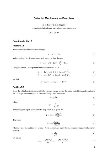
We know that a = 340km+6373km ≈ 7× 10 8 cm, ρ ≈ 10 −14 g cm −3 , and κ 2 = GM⊕ = 4×10 20 cm 3 s −2 ,
and we can estimate Cd ∼ 1, σ ∼ 50 × 50m 2 ≈ 3 × 10 7 cm 2 , and m ∼ 400t ≈ 4 × 10 8 g. (Don’t worry if
you took, say, σ = 1000m 2 and m = 100t — it’s fine for a rough estimate.) Substituting the numbers
into Eq. (11), we find
˙a ≈ −4 × 10 −1 cm s −1 ,
which translates to an altitude loss of roughly 400 meters per day or about 10 kilometers per month.
Figure 1 shows the real evolution of the ISS’s altitude, with the height loss (between the reboosts) being
consistent with our estimate.
Figure 1: “ This plot shows the orbital height of the ISS over one year. Clearly visible are the re-boosts
which suddenly increase the height, and the gradual decay in between. The height is averaged over one
orbit, and the gradual decrease is caused by atmospheric drag. As can be seen from the plot, the rate
of descent is not constant and this variation is caused by changes in the density of the tenuous outer
atmosphere due mainly to solar activity. ” (Source: www.heavens-above.com, 2011-12-07)
From our estimate, it follows that if the air density were by two orders of magnitude higher (ρ ∼
10 −12 g cm −3 ), the loss rate would be on order of hundreds of kilometers per month — comparable
with the altitude itself. Obviously, space flight at atmospheric layers that thick would no longer be possible.
Figure 2 shows the output of a commonly used average model for Earth’s atmosphere (Source:
http://modelweb.gsfc.nasa.gov/). The critical density of ρ ≈ 10 −12 g cm −3 discussed above
is reached at an altitude of ≈ 170km. There are indeed no satellites flying closer to the Earth surface
than that.
2
Density [g/cm 3 ]
0.01
1e-04
1e-06
1e-08
1e-10
1e-12
1e-14
1e-16
Atmospheric mass density
1e-18
0 200 400 600 800 1000
Altitude [km]
Figure 2: Average mass density of the atmosphere against altitude.