Game Theory: Repeated Games - Branislav L. Slantchev (UCSD)

Game Theory:
Repeated Games
Branislav L. Slantchev
Department of Political Science, University of California – San Diego
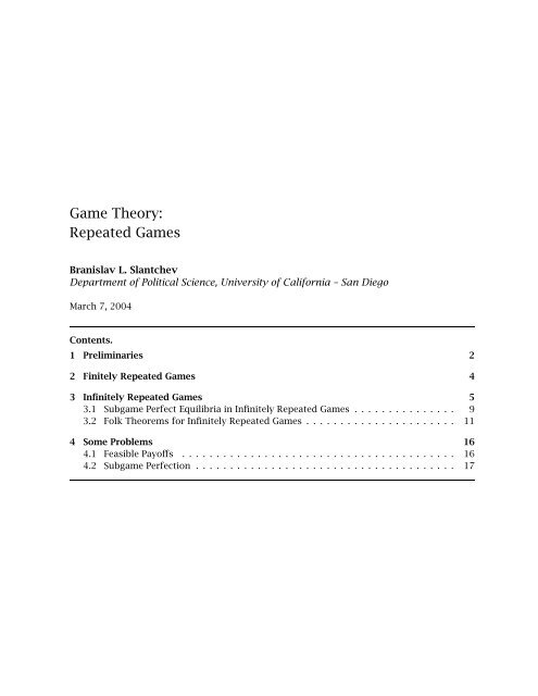
March 7, 2004
Contents.
1 Preliminaries 2
2 Finitely Repeated Games 4
3 Infinitely Repeated Games 5
3.1 SubgamePerfectEquilibriainInfinitelyRepeatedGames............... 9
3.2 FolkTheoremsforInfinitelyRepeatedGames...................... 11
4 Some Problems 16
4.1 FeasiblePayoffs ........................................ 16
4.2 SubgamePerfection...................................... 17

We have already seen an example of a finitely repeated game (recall the multi-stage game
where a static game with multiple equilibria was repeated twice). Generally, we would like
to be able to model situations where players repeatedly interact with each other. In such
situations, a player can condition his behavior at each point in the game on the other players’
past behavior. We have already seen what this possibility implies in extensive form games
(and we have obtained quite a few somewhat surprising results). We now take a look at a
class of games where players repeatedly engage in the same strategic game.
When engaged in a repeated situation, players must consider not only their short-term
gains but also their long-term payoffs. For example, if a Prisoner’s Dilemma is played once,
both players will defect. If, however, it is repeatedly played by the same two players, then
maybe possibilities for cooperation will emerge. The general idea of repeated games is that
players may be able to deter another player from exploiting his short-term advantage by
threatening punishment that reduces his long-term payoff.
We shall consider two general classes of repeated games: (a) games with finitely many
repetitions, and (b) games with infinite time horizons. Before we jump into theory, we need
to go over several mathematical preliminaries involving discounting.
1 Preliminaries
Let G =〈N,(Ai), (gi)〉 be an n-player normal form game. This is the building block of a
repeated game and is the game that is repeated. We shall call G the stage game. This can
be any normal form game, like Prisoner’s Dilemma, Battle of the Sexes, or anything else you
might conjure up. As before, assume that G is finite: that is it has a finite number of players
i, each with finite action space Ai, and a corresponding payoff function gi : A → R, where
A =△Ai.
The repeated game is defined in the following way. First, we must specify the players’
strategy spaces and payoff functions. The stage game is played at each discrete time period
t = 0, 1, 2,...,T and at the end of each period, all players observe the realized actions. The
game is finitely repeated if T

is any history of infinite length. Every nonterminal history begins a subgame in the repeated
game.
After any nonterminal history, all players i ∈ N simultaneously choose actions ai ∈ Ai.
Because every player observes h t ,apure strategy for player i in the repeated game is a
sequence of functions, si(h t ) : H t → Ai, that assign possible period-t histories h t ∈ H t to
actions ai ∈ Ai. That is, si(h t ) denotesanactionai for player i after history h t . So, a
strategy for player i is just
si =
si(h 0 ), si(h 1 ),...,si(h T
)
where it may well be the case that T =∞. For example, in the RPD game, a strategy may
specify
si(h 0 ) = C
si(h t ⎧
⎪⎨ C if a
) =
⎪⎩
τ
j = C,j ≠ i, for τ = 0, 1,...,t− 1
D otherwise
This strategy will read: “begin by cooperating in the first period, then cooperate as long as
the other player has cooperated in all previous periods, defect otherwise.” (This strategy is
called the grim-trigger strategy because even one defection triggers a retaliation that lasts
forever.)
Denote the set of strategies for player i by Si and the set of all strategy profiles by S =△Si.
A mixed (behavior) strategy σi for player i is a sequence of functions, σi(ht ) : Ht →Ai,
that map possible period-t histories to mixed actions αi ∈Ai (where Ai is the space of
probability distributions over Ai). It is important to note that a player’s strategy cannot
depend on past values of his opponent’s randomizing probabilities but only on the past
values of a−i. Note again that each period begins a new subgame and because all players
choose actions simultaneously, these are the only proper subgames. This fact will be useful
when testing for subgame perfection.
We now define the players’ payoff functions for infinitely repeated games (for finitely repeated
games, the payoffs are usually taken to be the time average of the per-period payoffs).
Since the only terminal histories are the infinite ones and because each period’s payoff is
the payoff from the stage game, we must describe how players evaluate infinite streams of
payoffs of the form gi(a0 ), gi(a1
),... . There are several alternative specifications in the
literature but we shall focus on the case where players discount future utilities using a discount
factor δ ∈ (0, 1). Player i’s payoff for the infinite sequence a0 ,a1
,... is given by the
discounted sum of per-period payoffs:
ui = gi(a 0 ) + δgi(a 1 ) + δ 2 gi(a 2 ) +···+δ t gi(a t ∞
) +···= δ t gi(a t )
For any δ ∈ (0, 1), the constant stream of payoffs (c,c,c,...) yields the discounted sum1 ∞
δ t c = c
1 − δ
t=0
1 It is very easy to derive the formula. First, note that we can factor out c because it’s a constant. Second, let
z = 1 + δ + δ 2 + δ 3 + ... denote the sum of the infinite series. Now, δz = δ + δ 2 + δ 3 + δ 4 + ..., and therefore
z − δz = 1. But this now means that z = 1/(1 − δ), yielding the formula. Note that we had to use the fact that
δ ∈ (0, 1) to make this work.
3
t=0

If the player’s preferences are represented by the discounted sum of per-period payoffs, then
they are also represented by the discounted average of per-period payoffs:
ui = (1 − δ)
∞
δ t gi(a t ).
The normalization factor (1 − δ) serves to measure the repeated game payoffs and the stage
game payoffs in the same units. In the example with the constant stream of payoffs, the
normalized sum will be c, which is directly comparable to the payoff in a single period.
To be a little more precise, in the game denoted by G(δ), player i’s payoff function is to
maximize the normalized sum
ui = Eσ (1 − δ)
t=0
∞
δ t gi(σ (h t )),
t=0
where Eσ denotes the expectation with respect to the distribution over infinite histories generated
by the strategy profile σ . For example, since gi(C, C) = 2, the payoff to perpetual
cooperation is given by
ui = (1 − δ)
∞
t=0
δ t (2) = (1 − δ) 2
= 2.
1 − δ
This is why averaging makes comparisons easier: the payoff of the overall game G(δ) is
directly comparable to the payoff from the constituent (stage) game G because it is expressed
in the same units.
To recapitulate the notation, ui, si, andσi denote the payoffs, pure strategies, and mixed
strategies for player i in the overall game, while gi, ai, andαi denote the payoffs, pure
strategies, and mixed strategies in the stage game.
Finally, recall that each history starts a new proper subgame. This means that for any
strategy profile σ and history h t , we can compute the players’ expected payoffs from period
t onward. We shall call these the continuation payoffs, and re-normalize so that the
continuation payoffs from time t are measured in time-t units:
ui(σ |h t ) = (1 − δ)
∞
δ τ−t gi(σ (h t )).
With this re-normalization, the continuation payoff of a player who will receive a payoff of 1
per period from period t onward is 1 for any period t.
2 Finitely Repeated Games
These games represent the case of a fixed time horizon T

C D
C 2,2 0,3
D 3,0 1,1
Figure 1: The Stage Game: Prisoner’s Dilemma.
how the payoffs vary with different time horizons, we normalize them in units used for the
per-period payoffs. The average discounted payoff is
ui =
1 − δ
1 − δT +1
T
δ t gi(a t ).
To see how this works, consider the payoff from both players cooperating for all T periods.
The discounted sum without the normalization is
T
δ t (2) =
t=0
t=0
1 − δT +1
1 − δ (2),
while with the normalization, the average discounted sum is simply 2.
Let’s now find the subgame perfect equilibrium (equilibria?) of the Finitely Repeated Prisoner’s
Dilemma (FRPD) game. Since the game has a finite time horizon, we can apply backward
induction. In period T , the only Nash equilibrium is (D, D), and so both players defect.
Since both players will defect in period T , the only optimal action in period T − 1 is to defect
as well. Thus, the game unravels from its endpoint, and the only subgame perfect equilibrium
is the strategy profile where each player always defects. The outcome in every period
of the game is (D, D), and the payoffs in the FRPD are (1, 1).
With some more work, it is possible to show that every Nash equilibrium of the FRPD
generates the always defect outcome. To see this, let σ ∗ denote some Nash equilibrium.
Both players will defect in the last period T for any history h T that has positive probability
under σ ∗ because doing so increases their period-T payoff and because there are no future
periods in which they might be punished. Since players will always defect in the last period
along the equilibrium path, if player i conforms to his equilibrium strategy in period T − 1,
his opponent will defect at time T , and therefore player i has no incentive not to defect in
T − 1. An induction argument completes the proof.
Although there are several applications of finitely repeated games, the “unraveling” effect
makes them less suitable for modeling repeated situations than the games we now turn to.
3 Infinitely Repeated Games
These games represent the case of an infinite time horizon T =∞and are meant to model
situations where players are unsure about when precisely the game will end. The set of
equilibria of an infinitely repeated game can be very different from that of the corresponding
finitely repeated game because players can use self-enforcing rewards and punishments that
do not unravel from the terminal date. In particular, because there is no fixed last period of
the game, in which both players will surely defect, in the Repeated Prisoner’s Dilemma (RPD)
game players may be able to sustain cooperation by the threat of “punishment” in case of
defection.
5

While in the finitely repeated games case a strategy can explicitly state what to do in each
of the T periods, specifying strategies for infinitely repeated games is trickier because it must
specify actions after all possible histories, and there is an infinite number of these. Here are
the specifications of several common strategies.
• Always Defect (ALL-D). This strategy prescribes defecting after every history no matter
what the other player has done. So, si(h t ) = D for all t = 0, 1,....
• Always Cooperate (ALL-C). This strategy prescribes cooperating after every history no
matter what the other player has done. So, si(h t ) = C for all t = 0, 1,....
• Naïve Grim Trigger (N-GRIM). This strategy prescribes cooperating while the other
player cooperates and, should the other player defect even once, defect forever thereafter:
si(h t ⎧
⎪⎨
C if t = 0
) = C if a
⎪⎩
τ
j = C,j ≠ i, for τ = 0, 1,...,t− 1
D otherwise
This is a very unforgiving strategy that punishes a single deviation forever. However, it
only punishes deviations by the other player. The following strategy punishes even the
player’s own past deviations.
• Grim Trigger (GRIM). This strategy prescribes cooperating in the initial period and then
cooperating as long as both players cooperated in all previous periods:
si(h t ⎧
⎪⎨
C if t = 0
) = C if a
⎪⎩
τ = (C, C) for τ = 0, 1,...,t− 1
D otherwise
Unlike N-GRIM, this strategy “punishes” the player for his own deviations, not just the
deviations of the other player.
• Tit-for-Tat (TFT). This strategy prescribes cooperation in the first period and then playing
whatever the other player did in the previous period: defect if the other player
defected, and cooperate if the other player cooperated:
si(h t ⎧
⎪⎨
C if t = 0
) = C if a
⎪⎩
t−1
j = C,j ≠ i
D otherwise
This is the most forgiving retaliatory strategy: it punishes one defection with one defection
and restores cooperation immediately after the other player has resumed cooperating.
• Limited Retaliation (LR-K). This strategy, also known as Forgiving Trigger, prescribes
cooperation in the first period, and then k periods of defection for every defection of
any player, followed by reverting to cooperation no matter what has occurred during
the punishment phase:
6

1. Phase A: cooperate and switch to Phase B
2. Phase B: cooperate unless some player has defected in the previous period, in
which case switch to Phase C and set τ = 0;
3. Phase C: if τ ≤ k, setτ = τ + 1 and defect, otherwise switch to Phase A.
This retaliatory strategy fixes the number of periods with which to punish defection
but this is independent of the behavior of the other player. (In TFT, on the other hand,
the length of punishment depends on what the other player does while he is being
punished.)
• Pavlov (WS-LS). Also called, win-stay, lose-shift, this strategy prescribes cooperation in
the first period and then cooperation after any history in which the last outcome was
either (C, C) or (D, D) and defection otherwise:
si(h t ⎧
⎪⎨
C if t = 0
) = C if a
⎪⎩
t−1
∈ (C, C), (D, D)
D otherwise
This strategy chooses the same action if the last outcome was relatively good and
switches action if the last outcome was relatively bad for the player.
• Deviate Once (DEV1L). This strategy prescribes TFT until period L, then deviating in
period L, cooperating in period L + 1, and playing TFT thereafter.
si(h t ⎧
⎪⎨
C if t = 0ort = L + 1
,t ≠ L, L + 1) = C if a
⎪⎩
t−1
j = C,j ≠ i and t ≠ L
D otherwise
This retaliatory strategy attempts to exploit the opponent just once, if at all possible.
• Grim DEV1L. Play Grim Trigger until period L, then play D in period L and thereafter.
si(h t ⎧
⎪⎨
C if t = 0
,t

Let’s now work our way through a more interesting example. Is (GRIM, GRIM), the strategy
profile where both player use Grim Trigger, a Nash equilibrium? If both players follow GRIM,
the outcome will be cooperation in each period:
whose average discounted value is
(C,C),(C,C),(C,C),...,(C,C),...
∞
(1 − δ) δ t ∞
gi(C, C) = (1 − δ) δ t (2) = 2.
t=0
Consider the best possible deviation for player 1. For such a deviation to be profitable, it
must produce a sequence of action profiles which has defection by some players in some
period. If player 2 follows GRIM, he will not defect until player 1 defects, which implies that
a profitable deviation must involve a defection by player 1. Let τ where τ ∈{0, 1, 2,...}
be the first period in which player 1 defects. Since player 2 follows GRIM, he will play D
from period τ + 1 onward. Therefore, the best deviation for player 1 generates the following
sequence of action profiles: 2
t=0
(C,C),(C,C),...,(C,C) ,(D,C) ,(D,D),(D,D),...,
τ times
period τ
which generates the following sequence of payoffs for player 1:
2, 2,...,2,
3, 1, 1,....
τ times
The average discounted value of this sequence is3
(1 − δ) 2 + δ(2) + δ 2 (2) +···+δ τ−1 (2) + δ τ (3) + δ τ+1 (1) + δ τ+2
(1) +···
= (1 − δ)
= (1 − δ)
T −1
δ t (2) + δ T (3) +
t=0
(1 − δ T )(2)
1 − δ
= 2 + δ T T +1
− 2δ
∞
t=T +1
δ t
(1)
+ δ T (3) + δT +1 (1)
1 − δ
Solving the following inequality for δ yields the discount factor necessary to sustain cooperation:
2 + δ T − 2δ T +1 ≤ 2
δ T T +1
≤ 2δ
δ ≥ 1
2 .
2Note that the first profile is played τ times, from period 0 to period τ − 1 inclusive. That is, if τ = 3, the
(C, C) profile is played in periods 0, 1, and 2 (that is, 3 times). The sum of the payoffs will be τ−1 t=0 δt (2) =
2 t=0 δt (2). That is, notice that the upper limit is τ − 1.
3It might be useful to know that
whenever δ ∈ (0, 1).
T
δ t ∞
= δ t −
t=0
t=0
∞
t=T +1
δ t = 1
1 − δ
8
− δT +1
∞
δ t +1 1 − δT
=
1 − δ
t=0

In other words, for δ ≥ 1 /2, deviation is not profitable. This means that if players are sufficiently
patient (i.e. if δ ≥ 1 /2), then the strategy profile (GRIM, GRIM) is a Nash equilibrium of
the infinitely repeated PD. The outcome is cooperation in all periods.
It is fairly easy to see that the strategy profile in which both players play ALL-C cannot be
Nash equilibrium because each player can gain by deviating to ALL-D, for example.
3.1 Subgame Perfect Equilibria in Infinitely Repeated Games
At this point, it will be useful to recall the One-Shot Deviation Property (OSDP) that we previously
covered. We shall make heavy use of OSDP in the analysis of subgame perfect equilibria
of the RPD. Briefly, recall that a strategy profile (s ∗
i ,s∗ −i ) is a SPE of G(δ) if and only if no
player can gain by deviating once after any history and conform to his strategy thereafter.
1. Naïve Grim Trigger. Let’s check whether (N-GRIM,N-GRIM) is subgame perfect. To do
this, we only need to check whether it satisfies OSDP. Consider the history h 1 = (C, D),
that is, in the initial history, player 2 has defected. If player 2 now continues playing
N-GRIM, the sequence of action profiles will result (player 1 sticks to N-GRIM as well):
(D,C),(D,D),(D,D),...,
for which the payoffs are 0, 1, 1,..., whose discounted average value is δ. If player 2
deviates and plays D instead of C in period 1, he will get a payoff of 1 in every period,
whose discounted average value is 1. Since δt. This generates the following
9

sequence of action profiles:
(C,C),(C,C),...,(C,C) ,(C,D) ,(D,D),...,(D,D) ,(C,D) ,(D,D),(D,D),....
t times
period t T −t−1 times period T
The average discounted sum of this stream is 2 − 2δt + δt+1 + δT (δ − 1). (You should
verify this as well. 4 ) However, since δ − 1 < 0, this is strictly smaller than 2 − 2δt + δt+1 ,
and so such deviation is not profitable.
Because there are no other one-shot deviations to consider, player 1’s strategy is subgame
perfect. Similar calculations show that player 2’s strategy is also optimal, and so
(GRIM,GRIM) is a subgame perfect equilibrium of RPD as long as δ ≥ 1 /2.
The Grim Trigger strategy is very fierce in its punishment. The Limited Retaliation
and Tit-for-Tat strategies are much less so. However, we can show that these, too, can
sustain cooperation.
3. Limited Retaliation. Suppose the game is in the cooperative phase (either no deviations
have occurred or all deviations have been punished). We have to check whether there
exists a profitable one-shot deviation in this phase. Suppose player 2 follows LR-K. If
player 1 follows LR-K as well, the outcome will be (C, C) in every period, which yields
an average discounted payoff of 2. If player 1 deviates to D once and then follows the
strategy, the following sequence of action profiles will result:
(D,C),(D,D),(D,D),...,(D,D) ,(C,C),(C,C),...,
k times
with the following average discounted payoff:
(1 − δ) 3 + δ + δ 2 +···+δ k +
∞
t=k+1
δ t
(2) = 3 − 2δ + δ k+1
Therefore, there will be no profitable one-shot deviation in the cooperation phase if and
only if
3 − 2δ + δ k+1 ≤ 2
δ k+1 − 2δ + 1 ≤ 0
So, if, for example, k = 1, then this condition is (δ−1) 2 ≤ 0, which, of course, can never
be satisfied since δ

We now have to check if there is a profitable one-shot deviation in the punishment
phase. Suppose there are k ′

Definition 1. The payoffs (v1,v2,...,vn) is feasible in the stage game G if they are a convex
combination of the pure-strategy payoffs in G. The set of feasible payoffs is
V = convex hull v|∃a ∈ A with g(a) = v .
In other words, payoffs are feasible if they are a weighted average (the weights are all nonnegative
and sum to 1) of the pure-strategy payoffs. For example, the Prisoner’s Dilemma
in Fig. 1 (p. 5) has four pure-strategy payoffs, (2, 2), (0, 3), (3, 0), and(1, 1). These are all
feasible. Other feasible payoffs include the pairs (v, v) with v = α(1) + (1 − α)(2), with
α ∈ (0, 1), and the pairs (v1,v2) with v1 = α(0) + (1 − α)(3) with v1 + v2 = 3, which result
from averaging the payoffs (0, 3) and (3, 0). There are many other feasible payoffs that result
from averaging more than two pure-strategy payoffs. To achieve a weighted average of purestrategy
payoffs, the players can use a public randomization device. To achieve the expected
payoffs (1.5, 1.5), they could flip a fair coin and play (C, D) if it comes up heads and (D, C)
if it comes up tails.
The convex hull of a set of points is simply the smallest convex set containing all the
points. The set V is easier to illustrate with a picture. Let’s compute V for the stage game
shown to the left in Fig. 2 (p. 12). There are three pure-strategy payoffs in G, soweonly
need consider the convex hull of the set of three points, (−2, 2), (1, −2), and(0, 1), inthe
two-dimensional space.
L R
U −2, 2 1, −2
M 1, −2 −2, 2
D 0, 1 0, 1
v2
✻
(−2,
2)
❍
❙❍
❍
❙ ❍
❍
(0, 1)
❙ ❍
❙ ❇
❙ ❇
❙ ❇
❙ ❇
❙ ❇
❙ ❇
❙ ❇
❙❇ ❙❇
(1, −2)
✲v1
Figure 2: The Game G and the Convex Hull of its Pure-Strategy Payoffs.
As the plot on the right in Fig. 2 (p. 12) makes it clear, all points contained within the
triangle shown are feasible payoffs (the triangle is the convex hull).
Suppose now we consider a simple modification of the stage game, as shown in the payoff
matrix on the left in Fig. 3 (p. 13). In effect, we have added another pure-strategy payoff to
the game: (2, 3). What is the convex hull of these payoffs? As the plot on the right in Fig. 3
(p. 13) makes it clear, it is (again) the smallest convex set that contains all points. Note that
(0, 1) is now inside the set. All payoffs contained within the triangle are feasible payoffs.
We now proceed to define what we mean by “individually rational” payoffs. To do this, we
12

L R
U −2, 2 1, −2
M 1, −2 −2, 2
D 0, 1 2, 3
v2
✻
(2, 3)
(−2, 2)
✘ ❙
❙❙❙❙❙❙❙❙❙❙❙
(0, 1)
(1, −2)
✘✘✘✘✘✘ ✘✘✘✘✘ ☎
☎
☎
☎
☎
☎
☎
☎
☎
☎
☎
☎
☎
☎
✲v1
Figure 3: The Game G 2 and the Convex Hull of Its Pure-Strategy Payoffs.
must recall the minimax payoffs we discussed in the context of zero-sum games. 6 To remind
you, here’s the formal definition.
Definition 2. Player i’s reservation payoff or minimax value is
vi = min
α−i max gi(αi,α−i)
αi .
In other words, vi is the lowest payoff that player i’s opponents can hold him to by any
choice of α−i provided that player i correctly foresees α−i and plays a best response to it.
Let m i
−i be the minimax profile against player i, andletmi i be a strategy for player i such that
gi(m i
i ,mi −i ) = vi. That is, the strategy profile (m i
i ,mi −i ) yields player i’s minimax payoff in
G.
Let’s look closely at the definition. Consider the stage game G illustrated in Fig. 2 (p. 12).
To compute player 1’s minimax value, we first compute the payoffs to his pure strategies as
a function of player 2’s mixing probabilities. Let q be the probability with which player 2
chooses L. Player 1’s payoffs are then vU(q) =−3q +1, vM(q) = 3q −2, and vD(q) = 0. Since
player 1 can always guarantee himself a payoff of 0 by playing D, the question is whether
player 2 can hold him to this payoff by playing some particular mixture. Since q does not
enter vD, we can pick a value that minimizes the maximum of vU and vM, which occurs at
the point where the two expressions are equal, and so −3q + 1 = 3q − 2 ⇒ q = 1 /2. Since
vU( 1 /2) = vM( 1 /2) =−1 /2, player 1’s minimax value is 0. 7
Finding player 2’s minimax value is a bit more complicated because there are three pure
strategies for player 1 to consider. Let pU and pM denote the probabilities of U and M
6Or, as it might be in our case, did not discuss because we did not have time. Take a look at the lecture
notes.
7Note that max vU (q), vM(q) ≤ 0foranyq∈ [1/3, 2/3], so we can take any q in that range to be player
2’s minimax strategy against player 1.
13

espectively. Then, player 2’s payoffs are
vL(pU,pM) = 2(pU − pM) + (1 − pU − pM)
vR(pU,pM) =−2(pU − pM) + (1 − pU − pM),
and player 2’s minimax payoff may be obtained by solving
min max
pU ,pM
vL(pU,pM), vR(pU,pM) .
By inspection we see that player 2’s minimax payoff is 0, which is attained by the profile
1 1
2 , 2 , 0 . Unlike the case with player 1, the minimax profile here is uniquely determined:
If pU > pM, the payoff to L is positive, if pM > pU, the payoff to R is positive, and if
pU = pM < 1
2 , then both L and R have positive payoffs.
The minimax payoffs have special role because they determine the reservation utility of
the player. That is, they determine the payoff that players can guarantee themselves in any
equilibrium.
Observation 2. Player i’s payoff is at least v i in any static equilibrium and in any Nash
equilibrium of the repeated game regardless of the value of the discount factor.
This observation implies that no equilibrium of the repeated game can give player i apayoff
lower than his minimax value. We call any payoffs that Pareto dominate the minimax payoffs
individually rational. In the example game G, the minimax payoffs are (0, 0), and so the set of
individually rational payoffs consists of feasible pairs (v1,v2) such that v1 > 0andv2 > 0.
More formally,
Definition 3. The set of feasible strictly individually rational payoffs is the set
v ∈ V |vi >vi∀i .
In the example in Fig. 2 (p. 12), this set includes all points in the small right-angle triangle
cornered at (0, 0) and (0, 1).
We now state two very important results about infinitely repeated games. Both are called
“folk theorems” because the results were well-known to game theorists before anyone actually
formalized them, and so no one can claim credit. The first folk theorem shows that any
feasible strictly individually rational payoff vector can be supported in a Nash equilibrium of
the repeated game. The second folk theorem demonstrates a weaker result that any feasible
payoff vector that Pareto dominates any static equilibrium payoffs of the stage game can be
supported in a subgame perfect equilibrium of the repeated game.
Theorem 1 (A Folk Theorem). For every feasible strictly individually rational payoff vector
v, there exists a δ < 1 such that for all δ ∈ (δ, 1) there is a Nash equilibrium of G(δ) with
payoffs v.
The intuition of this theorem is simply that when the players are patient, any finite oneperiod
gain from deviation is outweighed by even a small loss in utility in every future period.
The proof constructs strategies that are unrelenting: A player who deviates will be minimaxed
in every subsequent period.
14

Proof. Assume there is a pure strategy profile a such that g(a) = v. 8 Consider the
following strategy for each player i: “Play ai in period 0 and continue to play ai as long
as (i) the realized action profile in the previous period was a, or (ii) the realized action in
the previous period differed from a in two or more components. If in some previous period
player i was the only one not to follow profile a, then each player j plays m i
j for the rest of
the game.”
Can player i gain by deviating from this profile? In the period in which he deviates, he
receives at most maxa gi(a) and since his opponents will minimax him forever after, he will
obtain vi in all periods thereafter. Thus, if player i deviates in period t, he obtains at most
(1 − δ t )vi + δ t (1 − δ) max
a gi(a) + δ t+1 v i.
To make this deviation unprofitable, we must find the value of δ such that this payoff is
strictly smaller than the payoff from following the strategy, which is vi:
(1 − δ t )vi + δ t (1 − δ) max
a gi(a) + δ t+1 v i

This inequality holds strictly at δ = 1, which means it is satisfied for a range of δ

Let p be the probability that player 1 chooses U and q be the probability that he chooses
M. Player 2’s expected payoff from L is p − 3q + 1, and his payoff from R is p + 5q − 3. By
inspection (or equating the payoffs), we find that p = q = 1 /2 is the worst player 1 can do to
player 2, in which case player 2’s minimax payoff is 0. The set of strictly rational payoffs is
the subset of feasible payoffs where u1 ≥− 1 /2 and u2 ≥ 0.
4.2 Subgame Perfection
Consider now an infinitely repeated game G(δ) with the stage game shown in Fig. 5 (p. 17).
C D
C 2,2 0,3
D 3,0 1,1
Figure 5: The Stage Game.
Are the following strategy profiles, as defined in the lecture notes, subgame perfect? Show
your work and calculate the minimum discount factors necessary to sustain the subgame
perfect equilibrium, if any.
• (TFT,TFT). Hint: partition payoffs and try using x = δ2 .
The game has four types of subgames, depending on the realization of the stage game
in the last period. To show subgame perfection, we must make sure neither player has
an incentive to deviate in any of these subgames.
1. The last realization was (C, C). 10 If player 1 follows TFT, then his payoff is
(1 − δ)[2 + 2δ + 2δ 2 + 2δ 3 +···] = 2.
If player 1 deviates, the sequence of outcomes is (D,C),(C,D),(D,C),(C,D),...,
and his payoff will be
(1 − δ)[3 + δ + 3δ 2 + δ 3 + 3δ 4 + δ 5 +···] = 3
1 + δ .
(Here we make use of the hint. The payoff can be partitioned into two sequences,
one in which the per-period payoff is 3, and another where the per-period payoff
is 1. So we have (letting x = δ2 as suggested):
10 This also handles the initial subgame.
3 + 0δ + 3δ 2 + 0δ 3 + 3δ 4 + 0δ 5 + 3δ 6 +···
= 3 + 3δ 2 + 3δ 4 + 3δ 6 +···+0δ + 0δ 3 + 0δ 5 +···
= 3[1 + δ 2 + δ 4 + δ 6 +···] + 0δ[1 + δ 2 + δ 4 +···]
= (3 + 0δ)[1 + δ 2 + δ 4 + δ 6 +···]
= 3[1 + x + x 2 + x 3 + x 4 +···]
1
= 3
1 − x
3
3
= =
1 − δ2 (1 − δ)(1 + δ)
17

Which gives you the result above when you multiply it by (1 − δ) to average it.
I have not gone senile. The reason for keeping the multiplication by 0 above is
just to let you see clearly how you would calculate it if the payoff from (C, D) was
something else.)
Deviation will not be profitable when 2 ≥ 3/(1 + δ), or whenever δ ≥ 1 /2.
2. The last realization was (C, D). If player 1 follows TFT, the resulting sequence of
outcomes will be (D,C),(C,D),(D,C),..., to which the payoff (as we just found
out above) is 3/(1 + δ). If player 1 deviates and cooperates, the sequence will be
(C,C),(C,C),(C,C),..., to which the payoff is 2. So, deviating will not be profitable
as long as 3/(1 + δ) ≥ 2, which means δ ≤ 1 /2. (We are already in hot water here:
Only δ = 1 /2 will satisfy both this condition and the one above!)
3. The last realization was (D, C). If player 1 follows TFT, the resulting sequence of
outcomes will be (C,D),(D,C),(C,D),.... Using the same method as before, we
find that the payoff to this sequence is 3δ/(1+δ). If player 1 deviates, the sequence
of outcomes will be (D,D),(D,D),(D,D),..., to which the payoff is 1. Deviation
will not be profitable whenever 3δ/(1 + δ) ≥ 1, which holds for δ ≥ 1 /2.
4. The last realization was (D, D). If player 1 follows TFT, the resulting sequence
of outcomes will be (D,D),(D,D),(D,D),..., to which the payoff is 1. If he deviates
instead, the sequence will be (C,D),(D,C),(C,D),...,towhichthepayoffis
3δ/(1 + δ). Deviation will not be profitable if 1 ≥ 3δ/(1 + δ), which is true only for
δ ≤ 1 /2.
It turns out that for (TFT,TFT) to be subgame perfect, it must be the case that δ = 1 /2, a
fairly hefty knife-edge requirement. In addition, it is an artifact of the way we specified
the payoffs. For example, changing the payoff from (D, C) to 4 instead of 3 results
in the payoff for the sequence of outcomes (D,C),(C,D),(D,C),... to be 4/(1 + δ).
To prevent deviation in case (a), we now want 2 ≥ 4/(1 + δ), which is only true if
δ ≥ 1, which is not possible. So, with this little change, the SPE disappears. For general
parameters, (TFT,TFT) is not subgame perfect, except for special cases where it may be
for some knife-edge value of δ. Therefore, TFT is not all that is so often cracked up to
be!
• (TFT,GRIM)
We first check the optimality of player 1’s strategy and then the optimality of player 2’s
strategy.
1. No deviations have occurred in the past. If player 1 follows TFT, the result is perpetual
cooperation, and the payoff is 2. If player 1 deviates, the resulting sequence
of outcomes is (D, C), (C, D), (D,D),.... The payoff is (1 − δ)[3 + ∞ t=2 δt ] =
3 − 3δ + δ2 . Deviation is not profitable whenever 1 − 3δ + δ2 ≤ 0, which is true for
any δ ≥ (3 − √ 5)/2.
Similarly, player 2’s payoff from following GRIM is 2. If player 2 deviates, the
sequence is (C,D),(D,D),(D,D),....Thepayoffis(1−δ)[3 + ∞ t=1 δt ] = 3 − 2δ.
This is not profitable for any δ ≥ 1 /2.
2. Player 2 has deviated in the previous period. If player 1 follows TFT, the sequence
of outcomes is perpetual defection, from which the payoff is 1. If player 1 deviates,
18

the sequence is (C,D),(D,D),..., for which the payoff is δ