Computer Models Define Tide Variability - NIWA

FEATURE
Computer Models Define
Tide Variability
by Derek Goring
The tide consists of as many as 600 harmonic constituents.
Of these components, however, eight are
primary tides—four diurnal (once daily) and four semidiurnal
(twice daily). Of these eight, just three semidiurnal
tides comprise more than 90% of the tidal energy in
most places. These three tides are the lunar,
solar, and elliptic, the last arising because the
moon’s orbit is elliptical rather than circular.
For most sites, you can forecast the tide to centimeter
accuracy in height and a few minutes
accuracy in time if you know just the eight primary
tide constituents.
We can accurately identify all eight constituents
by installing a tide gauge and recording
hourly data for 206 days, the time span between the
tides of highest range, called perigean spring tides, which
occur when a full or new moon coincides with the
moon’s closest approach to Earth. Once identified for a
particular location, hydrographers can use the eight constituents
to forecast or hindcast the tide at that site for
decades or even centuries. In some places, however, tides
Solving
complex
forecasting
problems
South
Island
D‘Urville
Island
Marlborough
Sounds
Cook
Strait
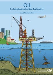
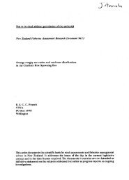
Figure 1. In this cotidal chart of Cook Strait for the primary lunar
semidiurnal tide (M2 ), colors denote the amplitude and lines denote
the time of high tide in hours after midnight on January 1, 1900.
OCTOBER/NOVEMBER 2001 © American Institute of Physics
Kapiti
Island
North
Island
40 km
14 The Industrial Physicist
along a coast can be quite different just short distances
apart. One such place is Cook Strait, between the North
and South Islands of New Zealand (Figure 1).
Along the southwestern coast of North Island, the
time of high tide varies by 3 h within a few kilometers,
although its amplitude is constant and only about 20
cm. However, along the western side of D’Urville Island
to the north of South Island, the time of high tide is constant
but the amplitude varies by 30 cm. This spatial
variability in the time and height of high tide is important
to the whole range of marine stakeholders, from
fishers to yachtsmen and from marine farmers to hydrographers.
Yet deploying tide gauges every few kilometers
along the coast is impractical for a country such as New
Zealand, which has an 11,000-km coastline but only 3.5
million people.
Applying physics
Using the two most basic laws of physics—conservation
of mass and conservation of momentum (Newton’s
second law)—and a lot of modern technology, we can
now solve the problem of defining the spatial
variability of tides.
Applying these two laws to fluid flow results
in a set of partial differential equations: a continuity
equation and the Navier–Stokes equations.
This complicated set of equations must be simplified
for most practical problems. First, we
eliminate turbulence by averaging to give the
Reynolds-averaged Navier–Stokes equations.
Then we apply a shallow-water assumption—the
simplification that the waves under consideration
are very long compared to the water depth.
Using this simplification, we can eliminate
the vertical dimension by integrating velocities
over depth and by assuming that the pressure
distribution over depth will be hydrostatic. This
results in a two-dimensional, time-varying problem
with three equations—a continuity equation
and two momentum equations—and three
unknowns: water surface displacement (η), and
eastward and northward depth-averaged velocities
(u and v). Because we are solving for tides,
which are harmonic, we can eliminate time by
converting all variables into the frequency
domain using Fourier transformation and solve for each
tide with its unique frequency in turn.
Special care must be taken with the two nonlinear

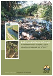
Figure 2. The area of each
triangular element of the
Cook Strait region is proportional
to the average depth
under it; long waves take
the same time to propagate
across all elements.
Figure 3. In this animation
sequence, velocity vectors
are shown for the Cook
Strait primary M2 tide over
selected time intervals.
terms (convective accelerations and
friction) to properly accommodate the
interactions between harmonic components,
because such interactions
generate harmonics at other frequencies.
In addition, for friction, the total velocity
for all tides must be used, not just the velocity
of the particular tide under consideration.
To accommodate these nonlinear effects, we
must iterate several times through the tides
until the solutions for all tides converge.
Transforming from the time domain to the
frequency domain involves substituting each
time-series variable with its harmonic equivalent.
For example, for the eastward velocity
we use u(t)=Ue i(ωt–φ), where t is time, U is
the amplitude, φ is the phase, ω is the angular
frequency of the tide under consideration,
and i = √–1. This makes all the unknown
variables complex with the form u r + iu i,
where u r = U cos φ is the real part and u i =
U sin φ is the imaginary part.
At one time, we would have had to solve
for real and imaginary parts separately, but
modern computer languages easily handle
complex numbers. The resulting problem
consists of three nonlinear, complex partial
differential equations in Cartesian coordinates.
To accommodate the curvature of the
Earth, however, these coordinates must be
transformed into spherical polar coordinates.
We discretize in space—that is, convert
from continuous variables in partial differential
equations to their numerical, or discrete,
equivalent—by using a finite-element
method. In this approach, we divide the geographical
domain of interest into a series of
triangles called “elements” (Figure 2) and
define the tide amplitude and eastward and
South
Island
northward velocities at each node of each triangle. Then,
for each element we evaluate the discretized differential
equations and assemble them into three global matrix
problems in η, u, and v. We solve these problems separately
and iteratively, first solving the continuity equation
for η using u and v from the previous iteration. Then we
solve the momentum equations for u and v using the
newly calculated values for η. We repeat this process
until the changes in the unknowns become negligible.
Boundary conditions
To drive the model, we need to apply boundary conditions,
which are the values of the unknown variables
applied at the boundary of the model domain. For these
conditions, we use results from the work of researchers
who have analyzed data from the U.S.–French oceanographic
satellite TOPEX/Poseidon. The satellite measures
the water surface displacement of the open ocean well
away from the continents. These data have been converted
into tidal constituents at 1º spacing around the globe
and are available to researchers.
Unfortunately, the satellite gives unreliable results
near land, and so we need a model that uses hydrodynamic
equations. Thus, for each of the tides in turn, we
apply the amplitude and phase (converted to complex
numbers) of the water level displacement from
TOPEX/Poseidon at the nodes around the open-ocean
boundary of the model. The solution gives us the amplitude
and phase for the three variables (η, u, and v) at
each of the 32,000 nodes in the model.
We repeat this process for 13 tidal constituents (8
major tides and 5 minor tides). Then, to accommodate the
nonlinear interactions between constituents and friction,
we solve again for the 13 tides using the previous results
15 The Industrial Physicist
North
Island
40 km

1
2
3
4
5
6
7
8
9
10
11
12
13
14
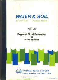
Figure 4. In this animation sequence, the primary M 2
tide amplitude is shown as it rotates counterclockwise
around both islands of New Zealand (red is
high, blue is low, green is zero elevation).
as starting points. We repeat
this iteration until we get
convergence for all 3 variables
at all 32,000 nodes and
for all 13 tides. With modern
computers and an efficient
matrix solver, this process
takes about 12 h on a 600-
MHz personal computer.
To check the results, we
have installed sea-level
recorders at 11 locations
around the New Zealand
coast (Figure 5a). These
highly accurate digital
recorders measure sea level
every 5 min to millimeter
accuracy. The sea-level
record contains information
not only about tides, but
also about storm surges,
tsunami, and long-term sealevel
changes. The recorders
are linked by cellular telephone
to our office, and we
download the data daily to
perform quality assurance
checks and archive the data.
Unlike many sea-level
recorders worldwide that
have been installed to assist
in navigation, this network
was commissioned for purely
scientific purposes. The
recorders have been installed
on the open coast, well away
from ports and harbors.
Thus, dredging or silting
does not affect them. Many
of the recorders are on islands
and must be serviced once or
twice a year by helicopter.
Others are on remote headlands
where overland access
is difficult, such as Anawhata
(Figure 5b), which is also
serviced by helicopter.
We analyze the data from
these 11 sites (and from
another 9 sites run by other
organizations) to generate
16 The Industrial Physicist
the amplitude and phase of the water-level displacement
for the 13 tides used, and we compare the results with
those from the model. When we first made this comparison,
we got a poor fit for some of the constituents. The
reason was that we did not take proper account of the
ocean-loading tide, which is the deflection of Earth’s crust
resulting from the change in the weight of the water above
it caused by the tide. In some places around New Zealand,
this crustal deflection is ±4 cm over a 12-h period and in
others, it is almost zero.
The model also overestimates the amplitude of the tide
at some places because we have not defined the sea-floor
topography or the shoreline accurately enough. This is
particularly true in harbors and estuaries where the tide is
locally amplified but the model tends to overestimate this
amplification if the grid is not fine enough. In most places
on the open coast, the model gets the tides right within
±10 cm in amplitude and ±10º in phase (equivalent to
±20 min for semidiurnal tides). This level of accuracy is
adequate for almost all applications of tide forecasting.
The accuracy of the model’s tidal currents is much
harder to verify. Measuring currents is a difficult task that
requires lowering valuable equipment over the side of a
ship and coming back several months later to recover it,
at which time you hope you can find where you put it
and that nobody has taken it. Furthermore, each current
meter measures the current at only one position in the
depth, but our model gives the average current over the
depth. Nevertheless, some records exist, and our model
provides results that are reasonable considering the simplifications
we have made to the governing equations to
make the problem tractable.
The results of the model are displayed as cotidal
charts (Figure 1) or they are synthesized into time slices
and animated (Figures 3 and 4).
Applications
We are using the model results in a wide range of
applications. One is to assist the police in recovering
bodies or other objects that have been thrown into the
sea. Using the velocities from the model, we can estimate
the journey that an object will undergo over a tidal cycle
(its excursion from one point and back). We plan to
extend this capability to tracking the propagation of oil
spills. Another application of the model is siting oil rigs
in the open ocean, where an accurate knowledge of the
tides greatly assists installation.
We also provide tidal corrections to hydrographers surveying
the bathymetry of the open ocean and coastal seas.
Marine farming of mussels is a booming industry in New
Zealand, and defining the tidal regime for new farms is

a b
important for their design and securing government permits.
We also provide a tide-forecasting service for any
location in the seas around New Zealand; our scientist
colleagues use this service to plan fieldwork and holidays.
Finally, we receive about one inquiry a week from
prospective brides planning a wedding on a remote
beach and trying to decide on which day and at what
time to have it.
Further reading
Cartwright, D. E. Tides: A Scientific History; Cambridge
University Press: Cambridge, England, 1999; 292 pp.
Pugh, D. T. Tides, Surges and Mean Sea-Level; John
Wiley & Sons: Chichester, England, 1987; 472 pp.
Walters, R. A. A model for tides and currents in the
English Channel and North Sea. Advances in Water
Resources 1987, 10, 138–148.
Visit www.amtec.com/contours/issue7/pom.html for
animated tidal-model results. Ω
B B I I O O G G R R A A P P H H Y
Y
Derek Goring is the principal scientist of the Coastal
Hydrodynamics Group of the National Institute of
Water and Atmospheric Research Ltd. in Christchurch,
New Zealand (d.goring@niwa.cri.nz).
Figure 5. A network
of 11 sea-level
recorders proivide
data used to verify
the tide model (a);
many are on islands
and remote headlands
and must be
serviced by helicopter
(b).