Lecture notes on linear algebra - Department of Mathematics ...

<strong>Lecture</strong> <strong>notes</strong> on linear algebra
David Lerner
Department of Mathematics
University of Kansas
These are <strong>notes</strong> of a course given in Fall, 2007 and 2008 to the Honors sections of our
elementary linear algebra course. Their comments and corrections have greatly improved
the exposition.
c○2007, 2008 D. E. Lerner

Contents
1 Matrices and matrix algebra 1
1.1 Examples of matrices . . . . . . . . . . . . . . . . . . . . . . . . . . . . . . . 1
1.2 Operations with matrices . . . . . . . . . . . . . . . . . . . . . . . . . . . . . 2
2 Matrices and systems of linear equations 7
2.1 The matrix form of a linear system . . . . . . . . . . . . . . . . . . . . . . . . 7
2.2 Row operations on the augmented matrix . . . . . . . . . . . . . . . . . . . . . 8
2.3 More variables . . . . . . . . . . . . . . . . . . . . . . . . . . . . . . . . . . . 9
2.4 The solution in vector notation . . . . . . . . . . . . . . . . . . . . . . . . . . 10
3 Elementary row operations and their corresponding matrices 12
3.1 Elementary matrices . . . . . . . . . . . . . . . . . . . . . . . . . . . . . . . . 12
3.2 The echelon and reduced echelon (Gauss-Jordan) form . . . . . . . . . . . . . . 13
3.3 The third elementary row operation . . . . . . . . . . . . . . . . . . . . . . . . 15
4 Elementary matrices, continued 16
4.1 Properties of elementary matrices . . . . . . . . . . . . . . . . . . . . . . . . . 16
4.2 The algorithm for Gaussian elimination . . . . . . . . . . . . . . . . . . . . . . 17
4.3 Observations . . . . . . . . . . . . . . . . . . . . . . . . . . . . . . . . . . . . 18
4.4 Why does the algorithm (Gaussian elimination) work? . . . . . . . . . . . . . . 19
4.5 Application to the solution(s) of Ax = y . . . . . . . . . . . . . . . . . . . . . 20
5 Homogeneous systems 23
5.1 Solutions to the homogeneous system . . . . . . . . . . . . . . . . . . . . . . . 23
5.2 Some comments about free and leading variables . . . . . . . . . . . . . . . . . 25
5.3 Properties of the homogenous system for Amn . . . . . . . . . . . . . . . . . . 26
5.4 Linear combinations and the superposition principle . . . . . . . . . . . . . . . . 27
6 The Inhomogeneous system Ax = y, y = 0 29
6.1 Solutions to the inhomogeneous system . . . . . . . . . . . . . . . . . . . . . . 29
6.2 Choosing a different particular solution . . . . . . . . . . . . . . . . . . . . . . 31
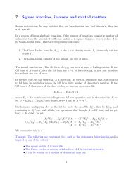
7 Square matrices, inverses and related matters 34
7.1 The Gauss-Jordan form of a square matrix . . . . . . . . . . . . . . . . . . . . 34
7.2 Solutions to Ax = y when A is square . . . . . . . . . . . . . . . . . . . . . . 36
7.3 An algorithm for constructing A −1 . . . . . . . . . . . . . . . . . . . . . . . . 36
i

8 Square matrices continued: Determinants 38
8.1 Introduction . . . . . . . . . . . . . . . . . . . . . . . . . . . . . . . . . . . . 38
8.2 Aside: some comments about computer arithmetic . . . . . . . . . . . . . . . . 38
8.3 The formal definition of det(A) . . . . . . . . . . . . . . . . . . . . . . . . . . 40
8.4 Some consequences of the definition . . . . . . . . . . . . . . . . . . . . . . . 40
8.5 Computations using row operations . . . . . . . . . . . . . . . . . . . . . . . . 41
8.6 Additional properties of the determinant . . . . . . . . . . . . . . . . . . . . . 43
9 The derivative as a matrix 45
9.1 Redefining the derivative . . . . . . . . . . . . . . . . . . . . . . . . . . . . . . 45
9.2 Generalization to higher dimensions . . . . . . . . . . . . . . . . . . . . . . . . 46
10 Subspaces 49
11 Linearly dependent and independent sets 53
11.1 Linear dependence . . . . . . . . . . . . . . . . . . . . . . . . . . . . . . . . . 53
11.2 Linear independence . . . . . . . . . . . . . . . . . . . . . . . . . . . . . . . . 54
11.3 Elementary row operations . . . . . . . . . . . . . . . . . . . . . . . . . . . . . 55
12 Basis and dimension of subspaces 56
12.1 The concept of basis . . . . . . . . . . . . . . . . . . . . . . . . . . . . . . . . 56
12.2 Dimension . . . . . . . . . . . . . . . . . . . . . . . . . . . . . . . . . . . . . 59
13 The rank-nullity (dimension) theorem 60
13.1 Rank and nullity of a matrix . . . . . . . . . . . . . . . . . . . . . . . . . . . . 60
13.2 The rank-nullity theorem . . . . . . . . . . . . . . . . . . . . . . . . . . . . . . 62
14 Change of basis 64
14.1 The coordinates of a vector . . . . . . . . . . . . . . . . . . . . . . . . . . . . 65
14.2 Notation . . . . . . . . . . . . . . . . . . . . . . . . . . . . . . . . . . . . . . 66
15 Matrices and Linear transformations 70
15.1 m × n matrices as functions from R n to R m . . . . . . . . . . . . . . . . . . . 70
15.2 The matrix of a linear transformation . . . . . . . . . . . . . . . . . . . . . . . 73
15.3 The rank-nullity theorem - version 2 . . . . . . . . . . . . . . . . . . . . . . . . 74
15.4 Choosing a useful basis for A . . . . . . . . . . . . . . . . . . . . . . . . . . . 75
16 Eigenvalues and eigenvectors 77
16.1 Definition and some examples . . . . . . . . . . . . . . . . . . . . . . . . . . . 77
16.2 Computations with eigenvalues and eigenvectors . . . . . . . . . . . . . . . . . 78
16.3 Some observations . . . . . . . . . . . . . . . . . . . . . . . . . . . . . . . . . 80
16.4 Diagonalizable matrices . . . . . . . . . . . . . . . . . . . . . . . . . . . . . . 81
17 Inner products 84
17.1 Definition and first properties . . . . . . . . . . . . . . . . . . . . . . . . . . . 84
17.2 Euclidean space . . . . . . . . . . . . . . . . . . . . . . . . . . . . . . . . . . 86
ii

18 Orthonormal bases and related matters 89
18.1 Orthogonality and normalization . . . . . . . . . . . . . . . . . . . . . . . . . . 89
18.2 Orthonormal bases . . . . . . . . . . . . . . . . . . . . . . . . . . . . . . . . . 90
19 Orthogonal projections and orthogonal matrices 93
19.1 Orthogonal decompositions of vectors . . . . . . . . . . . . . . . . . . . . . . . 93
19.2 Algorithm for the decomposition . . . . . . . . . . . . . . . . . . . . . . . . . . 94
19.3 Orthogonal matrices . . . . . . . . . . . . . . . . . . . . . . . . . . . . . . . . 96
19.4 Invariance of the dot product under orthogonal transformations . . . . . . . . . 97
20 Projections onto subspaces and the Gram-Schmidt algorithm 99
20.1 Construction of an orthonormal basis . . . . . . . . . . . . . . . . . . . . . . . 99
20.2 Orthogonal projection onto a subspace V . . . . . . . . . . . . . . . . . . . . . 100
20.3 Orthogonal complements . . . . . . . . . . . . . . . . . . . . . . . . . . . . . 102
20.4 Gram-Schmidt - the general algorithm . . . . . . . . . . . . . . . . . . . . . . . 103
21 Symmetric and skew-symmetric matrices 105
21.1 Decomposition of a square matrix into symmetric and skew-symmetric matrices . 105
21.2 Skew-symmetric matrices and infinitessimal rotations . . . . . . . . . . . . . . . 106
21.3 Properties of symmetric matrices . . . . . . . . . . . . . . . . . . . . . . . . . 107
22 Approximations - the method of least squares 111
22.1 The problem . . . . . . . . . . . . . . . . . . . . . . . . . . . . . . . . . . . . 111
22.2 The method of least squares . . . . . . . . . . . . . . . . . . . . . . . . . . . . 112
23 Least squares approximations - II 115
23.1 The transpose of A . . . . . . . . . . . . . . . . . . . . . . . . . . . . . . . . 115
23.2 Least squares approximations – the Normal equation . . . . . . . . . . . . . . . 116
24 Appendix: Mathematical implications and notation 119
iii

To the student
These are lecture <strong>notes</strong> for a first course in linear algebra; the prerequisite is a good course
in calculus. The <strong>notes</strong> are quite informal, but they have been carefully read and criticized by
two sections of honors students, and their comments and suggestions have been incorporated.
Although I’ve tried to be careful, there are undoubtedly some errors remaining. If you find
any, please let me know.
The material in these <strong>notes</strong> is absolutely fundamental for all mathematicians, physical scientists,
and engineers. You will use everything you learn in this course in your further studies.
Although we can’t spend too much time on applications here, three important ones are
treated in some detail — the derivative (Chapter 9), Helmholtz’s theorem on infinitessimal
deformations (Chapter 21) and least squares approximations (Chapters 22 and 23).
These are <strong>notes</strong>, and not a textbook; they correspond quite closely to what is actually said
and discussed in class. The intention is for you to use them instead of an expensive textbook,
but to do this successfully, you will have to treat them differently:
• Before each class, read the corresponding lecture. You will have to read it carefully,
and you’ll need a pad of scratch paper to follow along with the computations. Some
of the “easy” steps in the computations are omitted, and you should supply them. It’s
not the case that the “important” material is set off in italics or boxes and the rest can
safely be ignored. Typically, you’ll have to read each lecture two or three times before
you understand it. If you’ve understood the material, you should be able to work most
of the problems. At this point, you’re ready for class. You can pay attention in class
to whatever was not clear to you in the <strong>notes</strong>, and ask questions.
• The way most students learn math out of a standard textbook is to grab the homework
assignment and start working, referring back to the text for any needed worked examples.
That won’t work here. The exercises are not all at the end of the lecture; they’re
scattered throughout the text. They are to be worked when you get to them. If you
can’t work the exercise, you don’t understand the material, and you’re just kidding
yourself if you go on to the next paragraph. Go back, reread the relevant material and
try again. Work all the unstarred exercises. If you can’t do something, get help,
or ask about it in class. Exercises are all set off by “ ♣ Exercise: ”, so they’re easy to
find. The ones with asterisks (*) are a bit more difficult.
• You should treat mathematics as a foreign language. In particular, definitions must
be memorized (just like new vocabulary words in French). If you don’t know what
the words mean, you can’t possibly do the math. Go to the bookstore, and get yourself
a deck of index cards. Each time you encounter a new word in the <strong>notes</strong> (you can tell,
because the new words are set off by “ Definition: ”), write it down, together
with its definition, and at least one example, on a separate index card. Memorize
the material on the cards. At least half the time when students make a mistake, it’s
because they don’t really know what the words in the problem mean.
• There’s an appendix on proofs and symbols; it’s not really part of the text, but you
iv

may want to check there if you come upon a symbol or some form of reasoning that’s
not clear.
• Along with definitions come proofs. Doing a proof is the mathematical analog of
going to the physics lab and verifying, by doing the experiment, that the period of
a pendulum depends in a specific way on its length. Once you’ve done the proof or
experiment, you really know it’s true; you’re not taking someone else’s word for it.
The proofs in this course are (a) relatively easy, (b) unsurprising, in the sense that the
subject is quite coherent, and (c) useful in practice, since the proof often consists of
an algorithm which tells you how to do something.
This may be a new approach for some of you, but, in fact, this is the way the experts learn
math and science: we read books or articles, working our way through it line by line, and
asking questions when we don’t understand. It may be difficult or uncomfortable at first,
but it gets easier as you go along. Working this way is a skill that must be mastered by any
aspiring mathematician or scientist (i.e., you).
v

To the instructor
These are lecture <strong>notes</strong> for our 2-credit introductory linear algebra course. They correspond
pretty closely to what I said (or should have said) in class. Two of our Math 291 classes
have gone over the <strong>notes</strong> rather carefully and have made many useful suggestions which have
been happily adopted. Although the <strong>notes</strong> are intended to replace the standard text for this
course, they may be somewhat abbreviated for self-study.
How to use the <strong>notes</strong>: The way I’ve used the <strong>notes</strong> is simple: For each lecture, the students’
homework was to read the section (either a chapter or half of one) of the text that would
be discussed in class. Most students found this difficult (and somewhat unpleasant) at first;
they had to read the material three or four times before it began to make sense. They also
had to work (or at least attempt) all the unstarred problems before class. For most students,
this took between one and three hours of real work per class. During the actual class period,
I answered questions, worked problems, and tried to lecture as little as possible. This worked
quite well for the first half of the course, but as the material got more difficult, I found myself
lecturing more often - there were certain things that needed to be emphasized that might
not come up in a discussion format.
The students soon became accustomed to this, and even got to like it. Since this is the
way real scientists learn (by working though papers on their own), it’s a skill that must be
mastered — and the sooner the better.
Students were required to buy a 3 ×5 inch deck of index cards, to write down each definition
on one side of a card, and any useful examples or counterexamples on the back side. They
had to memorize the definitions: at least 25% of the points on each exam were definitions.
The only problems collected and graded were the starred ones. Problems that caused trouble
(quite a few) were worked out in class. There are not many standard “drill” problems.
Students were encouraged to make them up if they felt they needed practice.
Comments on the material: Chapters 1 through 8, covering the solution of linear algebraic
systems of equations, contains material the students have, in principle, seen before. But
there is more than enough new material to keep everyone interested: the use of elementary
matrices for row operations and the definition of the determinant as an alternating form are
two examples.
Chapter 9 (optional but useful) talks about the derivative as a linear transformation.
Chapters 10 through 16 cover the basic material on linear dependence, independence, basis,
dimension, the dimension theorem, change of basis, linear transformations, and eigenvalues.
The learning curve is fairly steep here; and this is certainly the most challenging part of the
course for most students. The level of rigor is reasonably high for an introductory course;
why shouldn’t it be?
Chapters 17 through 21 cover the basics of inner products, orthogonal projections, orthonormal
bases, orthogonal transformations and the connection with rotations, and diagonalization
of symmetric matrices. Helmholtz’s theorem (optional) on the infinitessimal motion of
a non-rigid body is used to motivate the decomposition of the derivative into its symmetric
vi

and skew-symmetric pieces.
Chapters 22 and 23 go over the motivation and simple use of the least squares approximation.
Most of the students have heard about this, but have no idea how or why it works. It’s a nice
application which is both easily understood and uses much of the material they’ve learned
so far.
Other things: No use was made of graphing calculators. The important material can all be
illustrated adequately with 2×2 matrices, where it’s simpler to do the computations by hand
(and, as an important byproduct, the students actually learn the algorithms). Most of our
students are engineers and have some acquaintance with MatLab, which is what they’ll use
for serious work, so we’re not helping them by showing them how to do things inefficiently.
In spite of this, every student brought a graphing calculator to every exam. I have no idea
how they used them.
No general definition of vector space is given. Everything is done in subspaces of R n , which
seems to be more than enough at this level. The disadvantage is that there’s no discussion
of vector space isomorphisms, but I felt that the resulting simplification of the exposition
justified this.
There are some shortcomings: The level of exposition probably varies too much; the demands
on the student are not as consistent as one would like. There should be a few more figures.
Undoubtedly there are typos and other minor errors; I hope there are no major ones.
vii

Chapter 1
Matrices and matrix algebra
1.1 Examples of matrices
Definition: A matrix is a rectangular array of numbers and/or variables. For instance
⎛
4 −2 0 −3
⎞
1
A = ⎝ 5 1.2 −0.7 x 3 ⎠
π −3 4 6 27
is a matrix with 3 rows and 5 columns (a 3 × 5 matrix). The 15 entries of the matrix are
referenced by the row and column in which they sit: the (2,3) entry of A is −0.7. We may
also write a23 = −0.7, a24 = x, etc. We indicate the fact that A is 3 × 5 (this is read as
”three by five”) by writing A3×5. Matrices can also be enclosed in square brackets as well as
large parentheses. That is, both
2 4
1 −6
and
are perfectly good ways to write this 2 × 2 matrix.
Real numbers are 1 × 1 matrices. A vector such as
⎛ ⎞
x
v = ⎝ y ⎠
z
2 4
1 −6
is a 3 × 1 matrix. We will generally use upper case Latin letters as symbols for general
matrices, boldface lower case letters for the special case of vectors, and ordinary lower case
letters for real numbers.
Definition: Real numbers, when used in matrix computations, are called scalars.
Matrices are ubiquitous in mathematics and the sciences. Some instances include:
1

• Systems of linear algebraic equations (the main subject matter of this course) are
normally written as simple matrix equations of the form Ax = y.
• The derivative of a function f : R 3 → R 2 is a 2 × 3 matrix.
• First order systems of linear differential equations are written in matrix form.
• The symmetry groups of mathematics and physics, some of which we’ll look at later,
are groups of matrices.
• Quantum mechanics can be formulated using infinite-dimensional matrices.
1.2 Operations with matrices
Matrices of the same size can be added or subtracted by adding or subtracting the corresponding
entries:
⎛ ⎞
2 1
⎛ ⎞
6 −1.2
⎛
8
⎞
−0.2
⎝ −3 4 ⎠ + ⎝ π x ⎠ = ⎝ π − 3 4 + x ⎠ .
7 0 1 −1 8 −1
Definition: If the matrices A and B have the same size, then their sum is the matrix A+B
defined by
(A + B)ij = aij + bij.
Their difference is the matrix A − B defined by
.
(A − B)ij = aij − bij
Definition: A matrix A can be multiplied by a scalar c to obtain the matrix cA, where
(cA)ij = caij.
This is called scalar multiplication. We just multiply each entry of A by c. For example
1 2 −3 −6
−3 =
3 4 −9 −12
Definition: The m × n matrix whose entries are all 0 is denoted 0mn (or, more often, just
by 0 if the dimensions are obvious from context). It’s called the zero matrix.
Definition: Two matrices A and B are equal if all their corresponding entries are equal:
A = B ⇐⇒ aij = bij for all i, j.
2

Definition: If the number of columns of A equals the number of rows of B, then the product
AB is defined by
k
(AB)ij = aisbsj.
s=1
Here k is the number of columns of A or rows of B.
If the summation sign is confusing, this could also be written as
Example:
1 2 3
−1 0 4
⎛
⎝
−1 0
4 2
1 3
⎞
(AB)ij = ai1b1j + ai2b2j + · · · + aikbkj.
⎠ =
1 · −1 + 2 · 4 + 3 · 1 1 · 0 + 2 · 2 + 3 · 3
−1 · −1 + 0 · 4 + 4 · 1 −1 · 0 + 0 · 2 + 4 · 3
=
10 13
5 12
If AB is defined, then the number of rows of AB is the same as the number of rows of A,
and the number of columns is the same as the number of columns of B:
Am×nBn×p = (AB)m×p.
Why define multiplication like this? The answer is that this is the definition that corresponds
to what shows up in practice.
Example: Recall from calculus (Exercise!) that if a point (x, y) in the plane is rotated
counterclockwise about the origin through an angle θ to obtain a new point (x ′ , y ′ ), then
x ′ = x cosθ − y sin θ
y ′ = x sin θ + y cos θ.
In matrix notation, this can be written
′ x
y ′
cosθ − sin θ
=
sin θ cosθ
x
y
If the new point (x ′ , y ′ ) is now rotated through an additional angle φ to get (x ′′ , y ′′ ), then
x ′′
y ′′
=
=
=
=
.
′
cosφ − sin φ x
sin φ cos φ y ′
cosφ − sin φ cosθ − sin θ
x
sin φ cosφ sin θ cosθ y
cosθ cosφ − sin θ sin φ −(cos θ sin φ + sin θ cosφ)
cosθ sin φ + sin θ cosφ cosθ cosφ − sin θ sin φ
cos(θ + φ) − sin(θ + φ) x
sin(θ + φ) cos(θ + φ) y
3
x
y

This is obviously correct, since it shows that the point has been rotated through the total
angle of θ +φ. So the right answer is given by matrix multiplication as we’ve defined it, and
not some other way.
Matrix multiplication is not commutative: in English, AB = BA, for arbitrary matrices
A and B. For instance, if A is 3 × 5 and B is 5 × 2, then AB is 3 × 2, but BA is not
defined. Even if both matrices are square and of the same size, so that both AB and BA
are defined and have the same size, the two products are not generally equal.
♣ Exercise: Write down two 2 × 2 matrices and compute both products. Unless you’ve been
very selective, the two products won’t be equal.
Another example: If
then
A =
AB =
2
3
2 4
3 6
, and B = 1 2 ,
, while BA = (8).
Two fundamental properties of matrix multiplication:
1. If AB and AC are defined, then A(B + C) = AB + AC.
2. If AB is defined, and c is a scalar, then A(cB) = c(AB).
♣ Exercise: * Prove the two properties listed above. (Both these properties can be proven by
showing that, in each equation, the (i, j) entry on the right hand side of the equation is equal
to the (i, j) entry on the left.)
Definition: The transpose of the matrix A, denoted At , is obtained from A by making the
first row of A into the first column of At , the second row of A into the second column of At ,
and so on. Formally,
= aji.
So ⎛
⎝
1 2
3 4
5 6
⎞
⎠
a t ij
t
=
1 3 5
2 4 6
Here’s one consequence of the non-commutatitivity of matrix multiplication: If AB is defined,
then (AB) t = B t A t (and not A t B t as you might expect).
Example: If
then
A =
AB =
2 1
3 0
2 7
−3 6
.
−1 2
, and B =
4 3
,
, so (AB) t
2 −3
=
7 6
4
.

And
as advertised.
B t A t =
−1 4
2 3
2 3
1 0
=
2 −3
7 6
♣ Exercise: ** Can you show that (AB) t = B t A t ? You need to write out the (i, j) th entry of
both sides and then observe that they’re equal.
Definition: A is square if it has the same number of rows and columns. An important
instance is the identity matrix In, which has ones on the main diagonal and zeros elsewhere:
Example:
⎛
I3 = ⎝
1 0 0
0 1 0
0 0 1
Often, we’ll just write I without the subscript for an identity matrix, when the dimension is
clear from the context. The identity matrices behave, in some sense, like the number 1. If
A is n × m, then InA = A, and AIm = A.
Definition: Suppose A and B are square matrices of the same dimension, and suppose that
AB = I = BA. Then B is said to be the inverse of A, and we write this as B = A−1 .
Similarly, B−1 = A. For instance, you can easily check that
2 1
1 1
1 −1
−1 2
=
⎞
⎠.
1 0
0 1
and so these two matrices are inverses of one another:
−1
2 1 1 −1 1 −1
= and
1 1 −1 2 −1 2
,
−1
Example: Not every square matrix has an inverse. For instance
3 1
A =
3 1
has no inverse.
=
2 1
1 1
♣ Exercise: * Show that the matrix A in the above example has no inverse. Hint: Suppose that
a b
B =
c d
is the inverse of A. Then we must have BA = I. Write this out and show that the equations
for the entries of B are inconsistent.
5
.

♣ Exercise: Which 1 × 1 matrices are invertible, and what are their inverses?
♣ Exercise: Show that if
a b
A =
c d
, and ad − bc = 0, then A −1 =
1
d −b
ad − bc −c a
Hint: Multiply A by the given expression for A −1 and show that it equals I. If ad − bc = 0,
then the matrix is not invertible. You should probably memorize this formula.
♣ Exercise: * Show that if A has an inverse that it’s unique; that is, if B and C are both
inverses of A, then B = C. (Hint: Consider the product BAC = (BA)C = B(AC).)
6
.

Chapter 2
Matrices and systems of linear equations
2.1 The matrix form of a linear system
You have all seen systems of linear equations such as
3x + 4y = 5
2x − y = 0. (2.1)
This system can be solved easily: Multiply the 2nd equation by 4, and add the two resulting
equations to get 11x = 5 or x = 5/11. Substituting this into either equation gives y = 10/11.
In this case, a solution exists (obviously) and is unique (there’s just one solution, namely
(5/11, 10/11)).
We can write this system as a matrix equation, in the form Ax = y:
3 4 x 5
= . (2.2)
2 −1 y 0
Here
x =
x
y
is called the coefficient matrix.
5
, and y =
0
3 4
, and A =
2 −1
This formula works because if we multiply the two matrices on the left, we get the 2 × 1
matrix equation 3x + 4y
2x − y
=
And the two matrices are equal if both their entries are equal, which holds only if both
equations in (2.1) are satisfied.
7
5
0
.

2.2 Row operations on the augmented matrix
Of course, rewriting the system in matrix form does not, by itself, simplify the way in which
we solve it. The simplification results from the following observation:
The variables x and y can be eliminated from the computation by simply writing down a
matrix in which the coefficients of x are in the first column, the coefficients of y in the second,
and the right hand side of the system is the third column:
3 4 5
2 −1 0
. (2.3)
We are using the columns as ”place markers” instead of x, y and the = sign. That is, the
first column consists of the coefficients of x, the second has the coefficients of y, and the
third has the numbers on the right hand side of (2.1).
We can do exactly the same operations on this matrix as we did on the original system 1 :
3 4 5
8 −4 0
3 4 5
11 0 5
3 4 5
5 1 0 11
: Multiply the 2nd eqn by 4
: Add the 1st eqn to the 2nd
: Divide the 2nd eqn by 11
The second equation now reads 1 · x + 0 · y = 5/11, and we’ve solved for x; we can now
substitute for x in the first equation to solve for y as above.
Definition: The matrix in (2.3) is called the augmented matrix of the system, and can
be written in matrix shorthand as (A|y).
Even though the solution to the system of equations is unique, it can be solved in many
different ways (all of which, clearly, must give the same answer). For instance, start with
the same augmented matrix 3 4 5
2 −1 0
1 5 5
2 −1 0
1 5 5
0 −11 −10
1 5 5
0 1 10
11
.
: Replace eqn 1 with eqn 1 - eqn 2
: Subtract 2 times eqn 1 from eqn 2
: Divide eqn 2 by -11 to get y = 10/11
1 The purpose of this lecture is to remind you of the mechanics for solving simple linear systems. We’ll
give precise definitions and statements of the algorithms later.
8

The second equation tells us that y = 10/11, and we can substitute this into the first equation
x + 5y = 5 to get x = 5/11. We could even take this one step further:
5 1 0 11
0 1 10
: We added -5(eqn 2) to eqn 1
11
The complete solution can now be read off from the matrix. What we’ve done is to eliminate
x from the second equation, (the 0 in position (2,1)) and y from the first (the 0 in position
(1,2)).
♣ Exercise: What’s wrong with writing the final matrix as
1 0 0.45
0 1 0.91
The system above consists of two linear equations in two unknowns. Each equation, by itself,
is the equation of a line in the plane and so has infinitely many solutions. To solve both
equations simultaneously, we need to find the points, if any, which lie on both lines. There
are 3 possibilities: (a) there’s just one (the usual case), (b) there is no solution (if the two
lines are parallel and distinct), or (c) there are an infinite number of solutions (if the two
lines coincide).
♣ Exercise: (Do this before continuing with the text.) What are the possibilities for 2 linear
equations in 3 unknowns? That is, what geometric object does each equation represent, and
what are the possibilities for solution(s)?
2.3 More variables
Let’s add another variable and consider two equations in three unknowns:
?
2x − 4y + z = 1
4x + y − z = 3 (2.4)
Rather than solving this directly, we’ll work with the augmented matrix for the system which
is 2 −4 1 1
4 1 −1 3
We proceed in more or less the same manner as above - that is, we try to eliminate x from
the second equation, and y from the first by doing simple operations on the matrix. Before
we start, observe that each time we do such an operation, we are, in effect, replacing the
original system of equations by an equivalent system which has the same solutions. For
instance, if we multiply the first equation by the number 2, we get a ”new” equation which
has exactly the same solutions as the original.
♣ Exercise: * This is also true if we replace, say, equation 2 with equation 2 plus some multiple
of equation 1. Why?
9
.

So, to business:
1 1 1 −2 2 2
4 1 −1 3
1 1 1 −2 2 2
0 9 −3 1
1 1 1 −2 2 2
0 1 −1
1
3 9
1 1 0 −
6
0 1 −1 3
13
18
1
9
: Mult eqn 1 by 1/2
: Mult eqn 1 by -4 and add it to eqn 2
: Mult eqn 2 by 1/9 (2.5)
: Add (2)eqn 2 to eqn 1 (2.6)
The matrix (2.5) is called an echelon form of the augmented matrix. The matrix (2.6) is
called the reduced echelon form. (Precise definitions of these terms will be given in the
next lecture.) Either one can be used to solve the system of equations. Working with the
echelon form in (2.5), the two equations now read
x − 2y + z/2 = 1/2
y − z/3 = 1/9.
So y = z/3 + 1/9. Substituting this into the first equation gives
x = 2y − z/2 + 1/2
= 2(z/3 + 1/9) − z/2 + 1/2
= z/6 + 13/18
♣ Exercise: Verify that the reduced echelon matrix (2.6) gives exactly the same solutions. This
is as it should be. All equivalent systems of equations have the same solutions.
2.4 The solution in vector notation
We see that for any choice of z, we get a solution to (2.4). Taking z = 0, the solution is
x = 13/18, y = 1/9. But if z = 1, then x = 8/9, y = 4/9 is the solution. Similarly for any
other choice of z which for this reason is called a free variable. If we write z = t, a more
familiar expression for the solution is
⎛
⎝
x
y
z
⎞
⎛
⎠ = ⎝
t 13 + 6 18
t 1
+ 3 9
t
⎞
⎛
⎠ = t ⎝
1
6
1
3
1
⎞
⎛
⎠ + ⎝
13
18 1
9
0
⎞
⎠ . (2.7)
This is of the form r(t) = tv + a, and you will recognize it as the (vector) parametric form
of a line in R 3 . This (with t a free variable) is called the general solution to the system
(??). If we choose a particular value of t, say t = 3π, and substitute into (2.7), then we have
a particular solution.
♣ Exercise: Write down the augmented matrix and solve these. If there are free variables, write
your answer in the form given in (2.7) above. Also, give a geometric interpretation of the
solution set (e.g., the common intersection of three planes in R 3 .)
10

1.
2.
3.
3x + 2y − 4z = 3
−x − 2y + 3z = 4
2x − 4y = 3
3x + 2y = −1
x − y = 10
x + y + 3z = 4
It is now time to think about what we’ve just been doing:
• Can we formalize the algorithm we’ve been using to solve these equations?
• Can we show that the algorithm always works? That is, are we guaranteed to get all
the solutions if we use the algorithm? Alternatively, if the system is inconsistent (i.e.,
no solutions exist), will the algorithm say so?
Let’s write down the different ‘operations’ we’ve been using on the systems of equations and
on the corresponding augmented matrices:
1. We can multiply any equation by a non-zero real number (scalar). The corresponding
matrix operation consists of multiplying a row of the matrix by a scalar.
2. We can replace any equation by the original equation plus a scalar multiple of another
equation. Equivalently, we can replace any row of a matrix by that row plus a multiple
of another row.
3. We can interchange two equations (or two rows of the augmented matrix); we haven’t
needed to do this yet, but sometimes it’s necessary, as we’ll see in a bit.
Definition: These three operations are called elementary row operations.
In the next lecture, we’ll assemble the solution algorithm, and show that it can be reformulated
in terms of matrix multiplication.
11

Chapter 3
Elementary row operations and their
corresponding matrices
3.1 Elementary matrices
As we’ll see, any elementary row operation can be performed by multiplying the augmented
matrix (A|y) on the left by what we’ll call an elementary matrix. Just so this doesn’t
come as a total shock, let’s look at some simple matrix operations:
• Suppose EA is defined, and suppose the first row of E is (1, 0, 0, . . ., 0). Then the first
row of EA is identical to the first row of A.
• Similarly, if the i th row of E is all zeros except for a 1 in the i th slot, then the i th row
of the product EA is identical to the i th row of A.
• It follows that if we want to change only row i of the matrix A, we should multiply A
on the left by some matrix E with the following property:
Every row except row i should be the i th row of the corresponding identity matrix.
The procedure that we illustrate below is used to reduce any matrix to echelon form (not
just augmented matrices). The way it works is simple: the elementary matrices E1, E2, . . .
are formed by (a) doing the necessary row operation on the identity matrix to get E, and
then (b) multiplying A on the left by E.
Example: Let
A =
3 4 5
2 −1 0
1. To multiply the first row of A by 1/3, we can multiply A on the left by the elementary
matrix
1
E1 = 3 0
.
0 1
12
.

(Since we don’t want to change the second row of A, the second row of E1 is the same
as the second row of I2.) The first row is obtained by multiplying the first row of I by
1/3. The result is
4 5 1
E1A = 3 3
2 −1 0
You should check this on your own. Same with the remaining computations.
2. To add -2(row1) to row 2 in the resulting matrix, multiply it by
E2 =
1 0
−2 1
The general rule here is the following: To perform an elementary row operation on
the matrix A, first perform the operation on the corresponding identity matrix
to obtain an elementary matrix; then multiply A on the left by this elementary
matrix.
3.2 The echelon and reduced echelon (Gauss-Jordan) form
Continuing with the problem, we obtain
1
E2E1A =
.
4 5
3
0 −
3
11
3 −10
3
Note the order of the factors: E2E1A and not E1E2A!
Now multiply row 2 of E2E1A by −3/11 using the matrix
yielding the echelon form
E3 =
1 0
0 − 3
11
4 1
E3E2E1A = 3
,
5
3
0 1 10
11
Last, we clean out the second column by adding (-4/3)(row 2) to row 1. The corresponding
elementary matrix is
4
1 −
E4 = 3 .
0 1
Carrying out the multiplication, we obtain the Gauss-Jordan form of the augmented matrix
E4E3E2E1A =
13
1 0 5
11
0 1 10
11
.
.
.
.

Naturally, we get the same result as before, so why bother? The answer is that we’re
developing an algorithm that will work in the general case. So it’s about time to formally
identify our goal in the general case. We begin with some definitions.
Definition: The leading entry of a matrix row is the first non-zero entry in the row,
starting from the left. A row without a leading entry is a row of zeros.
Definition: The matrix R is said to be in echelon form provided that
1. The leading entry of every non-zero row is a 1.
2. If the leading entry of row i is in position k, and the next row is not a row of zeros,
then the leading entry of row i + 1 is in position k + j, where j ≥ 1.
3. All zero rows are at the bottom of the matrix.
The following matrices are in echelon form:
⎛ ⎞
1 ∗ ∗
1 ∗
, ⎝ 0 0 1 ⎠ , and
0 1
0 0 0
⎛
⎝
0 1 ∗ ∗ ∗
0 0 1 ∗ ∗
0 0 0 1 ∗
Here the asterisks (*) stand for any number at all, including 0.
Definition: The matrix R is said to be in reduced echelon form if (a) R is in echelon
form, and (b) each leading entry is the only non-zero entry in its column. The reduced
echelon form of a matrix is also called the Gauss-Jordan form.
The following matrices are in reduced row echelon form:
⎛ ⎞ ⎛
1 ∗ 0 ∗ 0 1 0 0 ∗
1 0
, ⎝ 0 0 1 ∗ ⎠, and ⎝ 0 0 1 0 ∗
0 1
0 0 0 0 0 0 0 1 ∗
♣ Exercise: Suppose A is 3 × 5. What is the maximum number of leading 1’s that can appear
when it’s been reduced to echelon form? Same questions for A5×3. Can you generalize your
results to a statement for Am×n?. (State it as a theorem.)
Once a matrix has been brought to echelon form, it can be put into reduced echelon form
by cleaning out the non-zero entries in any column containing a leading 1. For example, if
⎛ ⎞
1 2 −1 3
R = ⎝ 0 1 2 0 ⎠,
0 0 0 1
which is in echelon form, then it can be reduced to Gauss-Jordan form by adding (-2)(row
2) to row 1, and then (-3)(row 3) to row 1. Thus
⎛ ⎞⎛
⎞
1 −2 0 1 2 −1 3
⎛ ⎞
1 0 −5 3
⎝ 0 1 0 ⎠⎝
0 1 2 0 ⎠ = ⎝ 0 1 2 0 ⎠.
0 0 1 0 0 0 1 0 0 0 1
14
⎞
⎠ .
⎞
⎠ .

and ⎛
⎝
1 0 −3
0 1 0
0 0 1
⎞⎛
⎠⎝
1 0 −5 3
0 1 2 0
0 0 0 1
⎞
⎛
⎠ = ⎝
1 0 −5 0
0 1 2 0
0 0 0 1
Note that column 3 cannot be ”cleaned out” since there’s no leading 1 there.
3.3 The third elementary row operation
There is one more elementary row operation and corresponding elementary matrix we may
need. Suppose we want to reduce the following matrix to Gauss-Jordan form
⎛
A = ⎝
2 2 −1
0 0 3
1 −1 2
Multiplying row 1 by 1/2, and then adding -row 1 to row 3 leads to
⎛
E2E1A = ⎝
1 0 0
0 1 0
−1 0 1
⎞ ⎛ ⎞ ⎛
1 0 0 2
⎠ ⎝ 0 1 0 ⎠ ⎝
0 0 1
⎞
⎠.
2 2 −1
0 0 3
1 −1 2
⎞
⎛
⎞
⎠.
1 1 − 1
2
5
2
⎞
⎠ = ⎝ 0 0 3 ⎠.
0 −2
Now we can clearly do 2 more operations to get a leading 1 in the (2,3) position, and another
leading 1 in the (3,2) position. But this won’t be in echelon form (why not?) We need to
interchange rows 2 and 3. This corresponds to changing the order of the equations, and
evidently doesn’t change the solutions. We can accomplish this by multiplying on the left
with a matrix obtained from I by interchanging rows 2 and 3:
⎛
E3E2E1A = ⎝
1 0 0
0 0 1
0 1 0
⎞ ⎛
1 1 −
⎠ ⎝
1 ⎞ ⎛
1 1 − 2
0 0 3 ⎠ = ⎝
0 −2
1 ⎞
2
5 0 −2 ⎠. 2
0 0 3
♣ Exercise: Without doing any written computation, write down the Gauss-Jordan form for
this matrix.
♣ Exercise: Use elementary matrices to reduce
2 1
A =
−1 3
to Gauss-Jordan form. You should wind up with an expression of the form
5
2
Ek · · ·E2E1A = I.
What is another name for the matrix B = Ek · · ·E2E1?
15

Chapter 4
Elementary matrices, continued
We have identified 3 types of row operations and their corresponding elementary matrices.
To repeat the recipe: These matrices are constructed by performing the given row operation
on the identity matrix:
1. To multiply rowj(A) by the scalar c use the matrix E obtained from I by multiplying
j th row of I by c.
2. To add (c)(rowj(A)) to rowk(A), use the identity matrix with its k th row replaced by
(. . .,c, . . ., 1, . . .). Here c is in position j and the 1 is in position k. All other entries
are 0
3. To interchange rows j and k, use the identity matrix with rows j and k interchanged.
4.1 Properties of elementary matrices
1. Elementary matrices are always square. If the operation is to be performed on
Am×n, then the elementary matrix E is m × m. So the product EA has the same
dimension as the original matrix A.
2. Elementary matrices are invertible. If E is elementary, then E −1 is the matrix
which undoes the operation that created E, and E −1 EA = IA = A; the matrix
followed by its inverse does nothing to A:
Examples:
•
E =
1 0
−2 1
adds (−2)(row1(A)) to row2(A). Its inverse is
E −1
1 0
=
2 1
16
,

♣ Exercise:
which adds (2)(row1(A)) to row2(A). You should check that the product of these
two is I2.
• If E multiplies the second row of a 2 × 2 matrix by 1,
then 2
E −1
1 0
= .
0 2
• If E interchanges two rows, then E = E−1 . For instance
0 1 0 1
= I
1 0 1 0
1. If A is 3 × 4, what is the elementary matrix that (a) subtracts (7)(row3(A)) from
row2(A)?, (b) interchanges the first and third rows? (c) multiplies row1(A) by 2?
2. What are the inverses of the matrices in exercise 1?
3. (*)Do elementary matrices commute? That is, does it matter in which order they’re
multiplied? Give an example or two to illustrate your answer.
4. (**) In a manner analogous to the above, define three elementary column operations
and show that they can be implemented by multiplying Am×n on the right by elementary
n × n column matrices.
4.2 The algorithm for Gaussian elimination
We can now formulate the algorithm which reduces any matrix first to row echelon form,
and then, if needed, to reduced echelon form:
1. Begin with the (1, 1) entry. If it’s some number a = 0, divide through row 1 by a to
get a 1 in the (1,1) position. If it is zero, then interchange row 1 with another row to
get a nonzero (1, 1) entry and proceed as above. If every entry in column 1 is zero,
go to the top of column 2 and, by multiplication and permuting rows if necessary, get
a 1 in the (1, 2) slot. If column 2 won’t work, then go to column 3, etc. If you can’t
arrange for a leading 1 somewhere in row 1, then your original matrix was the zero
matrix, and it’s already reduced.
2. You now have a leading 1 in some column. Use this leading 1 and operations of the
type (a)rowi(A) + rowk(A) → rowk(A) to replace every entry in the column below the
location of the leading 1 by 0. When you’re done, the column will look like
⎛ ⎞
1
⎜ 0.
⎟
⎜ ⎟
⎝ ⎠
0
.
17

3. Now move one column to the right, and one row down and attempt to repeat the
process, getting a leading 1 in this location. You may need to permute this row with
a row below it. If it’s not possible to get a non-zero entry in this position, move right
one column and try again. At the end of this second procedure, your matrix might
look like ⎛
⎝
1 ∗ ∗ ∗
0 0 1 ∗
0 0 0 ∗
where the second leading entry is in column 3. Notice that once a leading 1 has been
installed in the correct position and the column below this entry has been zeroed out,
none of the subsequent row operations will change any of the elements in the column.
For the matrix above, no subsequent row operations in our reduction process will
change any of the entries in the first 3 columns.
4. The process continues until there are no more positions for leading entries – we either
run out of rows or columns or both because the matrix has only a finite number of
each. We have arrived at the row echelon form.
The three matrices below are all in row echelon form:
⎛ ⎞
⎛ ⎞
1 ∗ ∗
⎛
1 ∗ ∗ ∗ ∗ ⎜ 0 0 1 ⎟
⎝ 0 0 1 ∗ ∗ ⎠ , or ⎜ 0 0 0 ⎟
⎟,
or ⎝
0 0 0 1 ∗ ⎝ 0 0 0 ⎠
0 0 0
⎞
⎠ ,
1 ∗ ∗
0 1 ∗
0 0 1
Remark: The description of the algorithm doesn’t involve elementary matrices. As a
practical matter, it’s much simpler to just do the row operation directly on A, instead of
writing down an elementary matrix and multiplying the matrices. But the fact that we could
do this with the elementary matrices turns out to be quite useful theoretically.
♣ Exercise: Find the echelon form for each of the following:
⎛ ⎞
1 2
⎜ 3 4 ⎟
⎝ 5 6 ⎠
7 8
,
0 4
, (3, 4),
7 −2
3 2 −1 4
2 −5 2 6
4.3 Observations
(1) The leading entries progress strictly downward, from left to right. We could just as easily
have written an algorithm in which the leading entries progress downward as we move from
right to left, or upwards from left to right. Our choice is purely a matter of convention, but
this is the convention used by most people.
Definition: The matrix A is upper triangular if any entry aij with i > j satisfies aij = 0.
18
⎞
⎠

(2) The row echelon form of the matrix is upper triangular
(3) To continue the reduction to Gauss-Jordan form, it is only necessary to use each leading
1 to clean out any remaining non-zero entries in its column. For the first matrix in (4.2)
above, the Gauss-Jordan form will look like
⎛
⎝
1 ∗ 0 0 ∗
0 0 1 0 ∗
0 0 0 1 ∗
Of course, cleaning out the columns may lead to changes in the entries labelled with *.
4.4 Why does the algorithm (Gaussian elimination) work?
Suppose we start with the system of equations Ax = y. The augmented matrix is (A|y),
where the coefficients of the variable x1 are the numbers in col1(A), the ‘equals’ sign is
represented by the vertical line, and the last column of the augmented matrix is the right
hand side of the system.
If we multiply the augmented matrix by the elementary matrix E, we get E(A|y). But this
can also be written as (EA|Ey).
Example: Suppose
(A|y) =
a b c
d e f
and we want to add two times the first row to the second, using the elementary matrix
The result is
E(A|y) =
E =
1 0
2 1
.
⎞
⎠
,
a b c
2a + d 2b + e 2c + f
But, as you can easily see, the first two columns of E(A|y) are just the entries of EA, and the
last column is Ey, so E(A|y) = (EA|Ey), and this works in general. (See the appropriate
problem.)
So after multiplication by E, we have the new augmented matrix (EA|Ey), which corresponds
to the system of equations EAx = Ey. Now suppose x is a solution to Ax = y.
Multiplication of this equation by E gives EAx = Ey, so x solves this new system. And
conversely, since E is invertible, if x solves the new system, EAx = Ey, multiplication by
E −1 gives Ax = y, so x solves the original system. We have just proven the
Theorem: Elementary row operations applied to either Ax = y or the corresponding augmented
matrix (A|y) don’t change the set of solutions to the system.
19
.

The end result of all the row operations on Ax = y takes the form
EkEk−1 · · ·E2E1Ax = Ek · · ·E1y,
or equivalently, the augmented matrix becomes
(EkEk−1 · · ·E2E1A|EkEk−1 · · ·E1y) = R,
where R is an echelon form of (A|y). And if R is in echelon form, we can easily work out
the solution.
4.5 Application to the solution(s) of Ax = y
Definition: A system of equations Ax = y is consistent if there is at least one solution x.
If there is no solution, then the system is inconsistent.
Suppose that we have reduced the augmented matrix (A|y) to either echelon or Gauss-Jordan
form. Then
1. If there is a leading 1 anywhere in the last column, the system Ax = y is inconsistent.
Why?
2. If there’s no leading entry in the last column, then the system is consistent. The
question then becomes “How many solutions are there?” The answer to this question
depends on the number of free variables:
Definition: Suppose the augmented matrix for the linear system Ax = y has been brought
to echelon form. If there is a leading 1 in any column except the last, then the corresponding
variable is called a leading variable. For instance, if there’s a leading 1 in column 3, then
x3 is a leading variable.
Definition: Any variable which is not a leading variable is a free variable.
Example: Suppose the echelon form of (A|y) is
1 3 3 −2
0 0 1 4
Then the original matrix A is 2 ×3, and if x1, x2, and x3 are the variables in the
original equations, we see that x1 and x3 are leading variables, and x2 is a free
variable. By definition, the number of free variables plus the number of leading
variables is equal to the number of columns of the matrix A.
20
.

• If the system is consistent and there are no free variables, then the solution
is unique — there’s just one. Here’s an example of this:
⎛ ⎞
1 ∗ ∗ ∗
⎜ 0 1 ∗ ∗ ⎟
⎝ 0 0 1 ∗ ⎠
0 0 0 0
• If the system is consistent and there are one or more free variables, then
there are infinitely many solutions.
⎛ ⎞
1 ∗ ∗ ∗
⎝ 0 0 1 ∗ ⎠
0 0 0 0
Here x2 is a free variable, and we get a different solution for each of the infinite number
of ways we could choose x2.
• Just because there are free variables does not mean that the system is
consistent. Suppose the reduced augmented matrix is
⎛ ⎞
1 ∗ ∗
⎝ 0 0 1 ⎠
0 0 0
Here x2 is a free variable, but the system is inconsistent because of the leading 1 in
the last column. There are no solutions to this system.
♣ Exercise: Reduce the augmented matrices for the following systems far enough so that you
can tell if the system is consistent, and if so, how many free variables exist. Don’t do any
extra work.
1.
2.
2x + 5y + z = 8
3x + y − 2z = 7
4x + 10y + 2z = 20
2x + 5y + z = 8
3x + y − 2z = 7
4x + 10y + 2z = 16
21

3.
4.
2x + 5y + z = 8
3x + y − 2z = 7
2x + 10y + 2z = 16
2x + 3y = 8
x − 4y = 7
Definition: A matrix A is lower triangular if all the entries above the main diagonal
vanish, that is, if aij = 0 whenever i < j.
♣ Exercise:
1. The elementary matrices which add k · rowj(A) to rowi(A), j < i are lower triangular.
Show that the product of any two 3 × 3 lower triangular matrices is again lower
triangular.
2. (**) Show that the product of any two n × n lower triangular matrices is lower triangular.
22

Chapter 5
Homogeneous systems
Definition: A homogeneous (ho-mo-jeen ′ -i-us) system of linear algebraic equations is one
in which all the numbers on the right hand side are equal to 0:
a11x1 + . . . + a1nxn = 0
. .
am1x1 + . . . + amnxn = 0
In matrix form, this reads Ax = 0, where A is m × n,
⎛ ⎞
and 0 is n × 1.
x =
⎜
⎝
x1
.
xn
⎟
⎠
n×1
5.1 Solutions to the homogeneous system
The homogenous system Ax = 0 always has the solution x = 0. It follows that any
homogeneous system of equations is consistent
Definition: Any non-zero solutions to Ax = 0, if they exist, are called non-trivial solutions.
These may or may not exist. We can find out by row reducing the corresponding augmented
matrix (A|0).
Example: Given the augmented matrix
⎛
1
⎞
2 0 −1 0
(A|0) = ⎝ −2 −3 4 5 0 ⎠ ,
2 4 0 −2 0
23
,

ow reduction leads quickly to the echelon form
⎛
⎞
1 2 0 −1 0
⎝ 0 1 4 3 0 ⎠ .
0 0 0 0 0
Observe that nothing happened to the last column — row operations do nothing to a column
of zeros. Equivalently, doing a row operation on a system of homogeneous equations doesn’t
change the fact that it’s homogeneous. For this reason, when working with homogeneous
systems, we’ll just use the matrix A, rather than the augmented matrix. The echelon form
of A is
⎛
⎝
1 2 0 −1
0 1 4 3
0 0 0 0
Here, the leading variables are x1 and x2, while x3 and x4 are the free variables, since there
are no leading entries in the third or fourth columns. Continuing along, we obtain the Gauss-
Jordan form (You should be working out the details on your scratch paper as we go along
....)
⎛
⎝
1 0 −8 −7
0 1 4 3
0 0 0 0
No further simplification is possible because any new row operation will destroy the structure
of the columns with leading entries. The system of equations now reads
⎞
⎠ .
⎞
⎠ .
x1 − 8x3 − 7x4 = 0
x2 + 4x3 + 3x4 = 0,
In principle, we’re finished with the problem in the sense that we have the solution in hand.
But it’s customary to rewrite the solution in vector form so that its properties are more
evident. First, we solve for the leading variables; everything else goes on the right hand side:
x1 = 8x3 + 7x4
x2 = −4x3 − 3x4.
Assigning any values we choose to the two free variables x3 and x4 gives us one the many
solutions to the original homogeneous system. This is, of course, why the variables are
called ”free”. For example, taking x3 = 1, x4 = 0 gives the solution x1 = 8, x2 = −4. We
can distinguish the free variables from the leading variables by denoting them as s, t, u,
24

etc. This is not logically necessary; it just makes things more transparent. Thus, setting
x3 = s, x4 = t, we rewrite the solution in the form
x1 = 8s + 7t
x2 = −4s − 3t
x3 = s
x4 = t
More compactly, the solution can also be written in matrix and set notation as
⎧⎛
⎪⎨ ⎜
xH = ⎜
⎝
⎪⎩
x1
x2
x3
x4
⎞
⎟
⎠ = s
⎛
⎜
⎝
8
−4
1
0
⎞
⎟
⎠ + t
⎛
⎜
⎝
7
−3
0
1
⎞
⎟
⎠
⎫
⎪⎬
: for all s, t ∈ R
⎪⎭
The curly brackets { } are standard notation for a set or collection of objects.
Definition: xH is called the general solution to the homogeneous equation.
(5.1)
Notice that xH is an infinite set of objects (one for each possible choice of s and t) and not
a single vector. The notation is somewhat misleading, since the left hand side xH looks like
a single vector, while the right hand side clearly represents an infinite collection of objects
with 2 degrees of freedom. We’ll improve this later.
5.2 Some comments about free and leading variables
Let’s go back to the previous set of equations
x1 = 8x3 + 7x4
x2 = −4x3 − 3x4.
Notice that we can rearrange things: we could solve the second equation for x3 to get
x3 = − 1
4 (x2 + 3x4),
and then substitute this into the first equation, giving
x1 = −2x2 + x4.
Now it looks as though x2 and x4 are the free variables! This is perfectly all right: the
specific algorithm (Gaussian elimination) we used to solve the original system leads to the
form in which x3 and x4 are the free variables, but solving the system a different way (which
is perfectly legal) could result in a different set of free variables. Mathematicians would
say that the concepts of free and leading variables are not invariant notions. Different
computational schemes lead to different results.
25

BUT ...
What is invariant (i.e., independent of the computational details) is the number of free
variables (2) and the number of leading variables (also 2 here). No matter how you solve the
system, you’ll always wind up being able to express 2 of the variables in terms of the other
2! This is not obvious. Later we’ll see that it’s a consequence of a general result called the
dimension or rank-nullity theorem.
The reason we use s and t as the parameters in the system above, and not x3 and x4 (or
some other pair) is because we don’t want the notation to single out any particular variables
as free or otherwise – they’re all to be on an equal footing.
5.3 Properties of the homogenous system for Amn
If we were to carry out the above procedure on a general homogeneous system Am×nx = 0,
we’d establish the following facts:
♣ Exercise:
• The number of leading variables is ≤ min(m, n).
• The number of non-zero equations in the echelon form of the system is equal to the
number of leading entries.
• The number of free variables plus the number of leading variables = n, the number of
columns of A.
• The homogenous system Ax = 0 has non-trivial solutions if and only if there are free
variables.
• If there are more unknowns than equations, the homogeneous system always has nontrivial
solutions. (Why?) This is one of the few cases in which we can tell something
about the solutions without doing any work.
• A homogeneous system of equations is always consistent (i.e., always has at least one
solution).
1. What sort of geometric object does xH represent?
2. Suppose A is 4 × 7. How many leading variables can Ax = 0 have? How many free
variables?
3. (*) If the Gauss-Jordan form of A has a row of zeros, are there necessarily any free
variables? If there are free variables, is there necessarily a row of zeros?
26

5.4 Linear combinations and the superposition principle
There are two other fundamental properties of the homogeneous system:
1. Theorem: If x is a solution to Ax = 0, then so is cx for any real number c.
Proof: x is a solution means Ax = 0. But A(cx) = c(Ax) = c0 = 0, so cx is
also a solution.
2. Theorem: If x and y are two solutions to the homogeneous equation, then so is x + y.
Proof: A(x + y) = Ax + Ay = 0 + 0 = 0, so x + y is also a solution.
These two properties constitute the famous principle of superposition which holds for
homogeneous systems (but NOT for inhomogeneous ones).
Definition: If x and y are vectors and s and t are scalars, then sx + ty is called a linear
combination of x and y.
Example: 3x − 4πy is a linear combination of x and y.
We can reformulate this as:
Superposition principle: if x and y are two solutions to the homogenous equation Ax =
0, then any linear combination of x and y is also a solution.
Remark: This is just a compact way of combining the two properties: If x and y are solutions,
then by property 1, sx and ty are also solutions. And by property 2, their sum sx + ty is a
solution. Conversely, if sx + ty is a solution to the homogeneous equation for all s, t, then
taking t = 0 gives property 1, and taking s = t = 1 gives property 2.
You have seen this principle at work in your calculus courses.
Example: Suppose φ(x, y) satisfies LaPlace’s equation
We write this as
∂2φ ∂x2 + ∂2φ = 0.
∂y2 ∆φ = 0, where ∆ = ∂2 ∂2
+
∂x2 ∂y2. The differential operator ∆ has the same property as matrix multiplication, namely: if
φ(x, y) and ψ(x, y) are two differentiable functions, and s and t are any two real numbers,
then
∆(sφ + tψ) = s∆φ + t∆ψ.
27

♣ Exercise: Verify this. That is, show that the two sides are equal by using properties of the
derivative. The functions φ and ψ are, in fact, vectors, in an infinite-dimensional space called
Hilbert space.
It follows that if φ and ψ are two solutions to Laplace’s equation, then any linear combination
of φ and ψ is also a solution. The principle of superposition also holds for solutions to the
wave equation, Maxwell’s equations in free space, and Schrödinger’s equation in quantum
mechanics. For those of you who know the language, these are all (systems of) homogeneous
linear differential equations.
Example: Start with ‘white’ light (e.g., sunlight); it’s a collection of electromagnetic waves
which satisfy Maxwell’s equations. Pass the light through a prism, obtaining red, orange,
..., violet light; these are also solutions to Maxwell’s equations. The original solution (white
light) is seen to be a superposition of many other solutions, corresponding to the various
different colors (i.e. frequencies). The process can be reversed to obtain white light again
by passing the different colors of the spectrum through an inverted prism. This is one of the
experiments Isaac Newton did when he was your age.
Referring back to the example (see Eqn (5.1)), if we set
x =
⎛
⎜
⎝
8
−4
1
0
⎞
⎛
⎞
7
⎟ ⎜
⎟
⎠ , and y = ⎜ −3 ⎟
⎝ 0 ⎠
1
,
then the susperposition principle tells us that any linear combination of x and y is also a
solution. In fact, these are all of the solutions to this system, as we’ve proven above.
28

Chapter 6
The Inhomogeneous system Ax = y, y = 0
Definition: The system Ax = y is inhomogeneous if it’s not homogeneous.
Mathematicians love definitions like this! It means of course that the vector y is not the zero
vector. And this means that at least one of the equations has a non-zero right hand side.
6.1 Solutions to the inhomogeneous system
As an example, we can use the same system as in the previous lecture, except we’ll change
the right hand side to something non-zero:
x1 + 2x2 − x4 = 1
−2x1 − 3x2 + 4x3 + 5x4 = 2
2x1 + 4x2 − 2x4 = 3
Those of you with sharp eyes should be able to tell at a glance that this system is inconsistent
— that is, there are no solutions. Why? We’re going to proceed anyway because this is hardly
an exceptional situation.
The augmented matrix is
⎛
(A|y) = ⎝
1 2 0 −1 1
−2 −3 4 5 2
2 4 0 −2 3
We can’t discard the 5th column here since it’s not zero. The row echelon form of the
augmented matrix is ⎛
⎞
1 2 0 −1 1
⎝ 0 1 4 3 4 ⎠ .
0 0 0 0 1
29
.
⎞
⎠ .

And the reduced echelon form is ⎛
⎝
1 0 −8 −7 0
0 1 4 3 0
0 0 0 0 1
The third equation, from either of these, now reads
⎞
⎠ .
0x1 + 0x2 + 0x3 + 0x4 = 1, or 0 = 1.
This is false! How can we wind up with a false statement? The actual reasoning that
led us here is this: If the original system has a solution, then performing elementary row
operations will give us an equivalent system with the same solution. But this equivalent
system of equations is inconsistent. It has no solutions; that is no choice of x1, . . ., x4
satisfies the equation. So the original system is also inconsistent.
In general: If the echelon form of (A|y) has a leading 1 in any position of the last column,
the system of equations is inconsistent.
Now it’s not true that any inhomogenous system with the same matrix A is inconsistent. It
depends completely on the particular y which sits on the right hand side. For instance, if
⎛ ⎞
1
y = ⎝ 2 ⎠ ,
2
then (work this out!) the echelon form of (A|y) is
and the reduced echelon form is
⎛
⎝
⎛
⎝
1 2 0 −1 1
0 1 4 3 4
0 0 0 0 0
1 0 −8 −7 −7
0 1 4 3 4
0 0 0 0 0
Since this is consistent, we have, as in the homogeneous case, the leading variables x1 and x2,
and the free variables x3 and x4. Renaming the free variables by s and t, and writing out
the equations solved for the leading variables gives us
⎞
⎠
x1 = 8s + 7t − 7
x2 = −4s − 3t + 4
x3 = s
x4 = t
30
⎞
⎠ .
.

This looks like the solution to the homogeneous equation found in the previous section except
for the additional scalars −7 and + 4 in the first two equations. If we rewrite this using
vector notation, we get
⎧⎛
⎪⎨ ⎜
xI = ⎜
⎝
⎪⎩
x1
x2
x3
x4
⎞
⎟
⎠ = s
⎛
⎜
⎝
8
−4
1
0
⎞
⎟
⎠ + t
⎛
⎜
⎝
7
−3
0
1
⎞
⎟
⎠ +
⎛
⎜
⎝
−7
4
0
0
⎞
⎟
⎠
⎫
⎪⎬
: ∀s, t ∈ R
⎪⎭
(The symbol ∀ is mathematical shorthand for the words for all or, equivalently, for any, or
for each, or for every).
Definition: xI is called the general solution to the inhomogeneous equation.
Compare this with the general solution xH to the homogenous equation found before. Once
again, we have a 2-parameter family (or set) of solutions. We can get a particular solution
by making some specific choice for s and t. For example, taking s = t = 0, we get the
particular solution
xp =
⎛
⎜
⎝
We can get other particular solutions by making other choices. Observe that the general
solution to the inhomogeneous system worked out here can be written in the form xI =
xH + xp. In fact, this is true in general:
Theorem: Let xp and ˆxp be two solutions to Ax = y. Then their difference xp − ˆxp is a solution
to the homogeneous equation Ax = 0. The general solution to Ax = y can be written as
xI = xp + xH where xH de<strong>notes</strong> the general solution to the homogeneous system.
Proof: Since xp and ˆxp are solutions, we have A(xp − ˆxp) = Axp − Aˆxp = y − y = 0. So
their difference solves the homogeneous equation. Conversely, given a particular solution
xp, then the entire set xp + xH consists of solutions to Ax = y: if z belongs to xH, then
A(xp + z) = Axp + Az = y + 0 = y and so xp + z is a solution to Ax = y.
−7
4
0
0
⎞
⎟
⎠ .
6.2 Choosing a different particular solution
Going back to the example, suppose we write the general solution to Ax = y in the vector
form
where
xI = {sv1 + tv2 + xp, ∀s, t ∈ R},
31

v1 =
⎛
⎜
⎝
8
−4
1
0
⎞
⎟
⎠ , v2 =
⎛
⎜
⎝
7
−3
0
1
⎞
⎟
⎠ , and xp =
Any different choice of s, t, for example taking s = 1, t = 1, gives another solution:
We can rewrite the general solution as
ˆxp =
⎛
⎜
⎝
8
−3
1
1
⎞
⎟
⎠ .
⎛
⎜
⎝
xI = (s − 1 + 1)v1 + (t − 1 + 1)v2 + xp
= (s − 1)v1 + (t − 1)v2 + ˆxp
= ˆsv1 + ˆtv2 + ˆxp
As ˆs and ˆt run over all possible pairs of real numbers we get exactly the same set of solutions
as before. So the general solution can be written as ˆxp +xH as well as xp +xH! This is a bit
confusing unless you recall that these are sets of solutions, rather than single solutions; (ˆs, ˆt)
and (s, t) are just different sets of coordinates. But running through either set of coordinates
(or parameters) produces the same set.
Remarks
• Those of you taking a course in differential equations will encounter a similar situation:
the general solution to a linear differential equation has the form y = yp + yh, where
yp is any particular solution to the DE, and yh de<strong>notes</strong> the set of all solutions to the
homogeneous DE.
• We can visualize the general solutions to the homogeneous and inhomogeneous equations
we’ve worked out in detail as follows. The set xH is a 2-plane in R 4 which goes
through the origin since x = 0 is a solution. The general solution to Ax = y is obtained
by adding the vector xp to every point in this 2-plane. Geometrically, this gives
another 2-plane parallel to the first, but not containing the origin (since x = 0 is not
a solution to Ax = y unless y = 0). Now pick any point in this parallel 2-plane and
add to it all the vectors in the 2-plane corresponding to xH. What do you get? You
get the same parallel 2-plane! This is why xp + xH = ˆxp + xH.
♣ Exercise: Using the same example above, let ˜xp be the solution obtained by taking s = 2, t =
−1. Verify that both xp − ˜xp and ˆxp − ˜xp are solutions to the homogeneous equation.
32
−7
4
0
0
.
⎞
⎟
⎠

xp
0
xp + z
Figure 6.1: The lower plane (the one passing through
0) represents xH; the upper is xI. Given the particular
solution xp and a z in xH, we get another solution to the
inhomogeneous equation. As z varies in xH, we get all
the solutions to Ax = y.
33
z
xH

Chapter 7
Square matrices, inverses and related matters
7.1 The Gauss-Jordan form of a square matrix
Square matrices are the only matrices that can have inverses, and for this reason, they are
a bit special.
In a system of linear algebraic equations, if the number of equations equals the number of
unknowns, then the associated coefficient matrix A is square. If we row reduce A to its
Gauss-Jordan form, there are two possible outcomes:
1. The Gauss-Jordan form for An×n is the n × n identity matrix In (commonly written
as just I).
2. The Gauss-Jordan form for A has at least one row of zeros.
The second case is clear: The GJ form of An×n can have at most n leading entries. If the
GJ form of A is not I, then the GJ form has n − 1 or fewer leading entries, and therefore
has at least one row of zeros.
In the first case, we can show that A is invertible. To see this, remember that A is reduced
to GJ form by multiplication on the left by a finite number of elementary matrices. If the
GJ form is I, then when all the dust settles, we have an expression like
EkEk−1 . . .E2E1A = I,
where Ek is the matrix corresponding to the k th row operation used in the reduction. If we
set B = EkEk−1 . . .E2E1, then clearly BA = I and so B = A −1 .
Furthermore, multiplying BA on the left by (note the order!!!) E −1
k
continuing to E −1
1
, then by E−1
k−1 , and
, we undo all the row operations that brought A to GJ form, and we get
back A. In detail, we get
(E −1
1 E −1
2 . . .E −1
k−1E−1 k
)BA = (E−1 1 E −1
2 . . .E −1
k−1E−1 k
(E −1
1 E−1 2 . . .E −1
k−1E−1 k )(EkEk−1 . . .E2E1)A = E −1
1 E−1 2 . . .E −1
k−1E−1 k
34
A = E −1
1 E −1
2 . . .E −1
k−1 E−1
k
)I or

We summarize this in a
Theorem: The following are equivalent (i.e., each of the statements below implies and is implied
by any of the others)
• The square matrix A is invertible.
• The Gauss-Jordan or reduced echelon form of A is the identity matrix.
• A can be written as a product of elementary matrices.
Example: - (fill in the details on your scratch paper)
We start with
A =
2 1
1 2
We multiply row 1 by 1/2 using the matrix E1:
E1A =
1
2 0
0 1
We now add -(row 1) to row 2, using E2:
1 0
E2E1A =
−1 1
Now multiply the second row by 2
3 :
1 0
E3E2E1A =
0 2
3
And finally, add − 1
2
So
♣ Exercise:
(row 2) to row 1:
E4E3E2E1A =
1 − 1
2
0 1
A =
.
1 1
2
1 2
1 1
2
0 3
2
1 1
2
1 2
=
1 1
2
0 1
=
.
1 1
2
0 3
2
=
A −1 = E4E3E2E1 = 1
2 −1
3 −1 2
1 1
2
0 1
.
1 0
0 1
• Check the last expression by multiplying the elementary matrices together.
• Write A as the product of elementary matrices.
• The individual factors in the product of A −1 are not unique. They depend on how we
do the row reduction. Find another factorization of A −1 . (Hint: Start things out a
different way, for example by adding -(row 2) to row 1.)
• Let
A =
1 1
2 3
Express both A and A −1 as the products of elementary matrices.
35
.
.
.
.

7.2 Solutions to Ax = y when A is square
• If A is invertible, then the equation Ax = y has the unique solution A −1 y for any right
hand side y. For,
Ax = y ⇐⇒ A −1 Ax = A −1 y ⇐⇒ x = A −1 y.
In this case, the solution to the homogeneous equation is also unique - it’s the trivial
solution x = 0.
• If A is not invertible, then there is at least one free variable (why?). So there are nontrivial
solutions to Ax = 0. If y = 0, then either Ax = y is inconsistent (the most
likely case) or solutions to the system exist, but there are infinitely many.
♣ Exercise: * If the square matrix A is not invertible, why is it ‘likely’ that the inhomogeneous
equation is inconsistent? ‘Likely’, in this context, means that the system should be
inconsistent for a y chosen at random.
7.3 An algorithm for constructing A −1
The work we’ve just done leads immediately to an algorithm for constructing the inverse
of A. (You’ve probably seen this before, but now you know why it works!). It’s based on
the following observation: suppose Bn×p is another matrix with the same number of rows as
An×n, and En×n is an elementary matrix which can multiply A on the left. Then E can also
multiply B on the left, and if we form the partitioned matrix
C = (A|B)n×(n+p),
Then, in what should be an obvious notation, we have
where EA is n × n and EB is n × p.
EC = (EA|EB)n×n+p,
♣ Exercise: Check this for yourself with a simple example. (*) Better yet, prove it in general.
The algorithm consists of forming the partitioned matrix C = (A|I), and doing the row
operations that reduce A to Gauss-Jordan form on the larger matrix C. If A is invertible,
we’ll end up with
Ek . . .E1(A|I) = (Ek . . .E1A|Ek . . .E1I)
= (I|A−1 .
)
In words: the same sequence of row operations that reduces A to I will convert I to A −1 .
The advantage to doing things this way is that we don’t have to write down the elementary
matrices. They’re working away in the background, as we know from the theory, but if all
we want is A −1 , then we don’t need them explicitly; we just do the row operations.
36

Example:
Then row reducing (A|I), we get
So,
(A|I) =
⎛
Let A = ⎝
r1 ↔ r2
do col 1
do column 2
and column 3
⎛
A −1 ⎜
= ⎜
⎝
⎛
⎝
⎛
⎝
⎛
⎝
1 2 3
1 0 −1
2 3 1
⎞
⎠ .
1 2 3 1 0 0
1 0 −1 0 1 0
2 3 1 0 0 1
1 0 −1 0 1 0
1 2 3 1 0 0
2 3 1 0 0 1
⎞
⎠
⎞
⎠
1 0 −1 0 1 0
0 2 4 1 −1 0
0 3 3 0 −2 1
⎞
⎠
⎛
1 0 −1 0 1 0
⎜ 1
⎜
0 1 2
⎜
2
⎝
−1
2 0
0 0 −3 − 3
2 −1
2 1
⎞
⎟
⎠
⎛
1 7
⎜
1 0 0
⎜ 2 6
⎜
⎝
−1
3
0 1 0 − 1
2 −5
2
6 3
1 1
0 0 1
2 6 −1
⎞
⎟
⎠
3
1
2
− 1
2 −5
6
1
2
7
6 −1
3
2
3
1
6 −1
3
♣ Exercise: Write down a 2 × 2 matrix and do this yourself. Same with a 3 × 3 matrix.
37
⎞
⎟ .
⎟
⎠

Chapter 8
Square matrices continued: Determinants
8.1 Introduction
Determinants give us important information about square matrices, and, as we’ll soon see, are
essential for the computation of eigenvalues. You have seen determinants in your precalculus
courses. For a 2 × 2 matrix
the formula reads
For a 3 × 3 matrix ⎛
⎝
A =
a b
c d
,
det(A) = ad − bc.
a11 a12 a13
a21 a22 a23
a31 a32 a33
life is more complicated. Here the formula reads
det(A) = a11a22a33 + a13a21a32 + a12a23a31 − a12a21a33 − a11a23a32 − a13a22a31.
Things get worse quickly as the dimension increases. For an n × n matrix A, the expression
for det(A) has n factorial = n! = 1 · 2 · . . .(n − 1) · n terms, each of which is a product of n
matrix entries. Even on a computer, calculating the determinant of a 10 × 10 matrix using
this sort of formula would be unnecessarily time-consuming, and doing a 1000 ×1000 matrix
would take years!
8.2 Aside: some comments about computer arithmetic
It is often the case that the simple algorithms and definitions we use in class turn out to be
cumbersone, inaccurate, and impossibly time-consuming when implemented on a computer.
There are a number of reasons for this:
38
⎞
⎠,

1. Floating point arithmetic, used on computers, is not at all the same thing as working
with real numbers. On a computer, numbers are represented (approximately!) in the
form
x = (d1d2 · · ·dn) × 2 a1a2···am ,
where n and m might be of the order 50, and d1 . . . am are binary digits (either 0 or1).
This is called the floating point representation (It’s the “decimal” point that floats -
you can represent the number 8 as 1000 × 2 0 , as 10 × 2 2 , etc.) As a simple example of
what goes wrong, suppose that n = 5. Then 19 = 1·2 4 +0·2 3 +0·2 2 +1·2 1 +1·2 0 , and
therefore has the binary representation 10011. Since it has 5 digits, it’s represented
correctly in our system. So is the number 9, represented by 1001. But the product
19 × 9 = 171 has the binary representation 10101011, which has 8 digits. We can only
keep 5 significant digits in our (admittedly primitive) representation. So we have to
decide what to do with the trailing 011 (which is 3 in decimal). We can round up
or down: If we round up we get 10111000 = 10110 × 2 3 = 176, while rounding down
gives 10101 × 2 3 = 168. Neither is a very good approximation to 171. Certainly a
modern computer does a better job than this, and uses much better algorithms, but
the problem, which is called roundoff error still remains. When we do a calculation
on a computer, we almost never get the right answer. We rely on something called
the IEEE standard to prevent the computer from making truly silly mistakes, but this
doesn’t always work.
2. Most people know that computer arithmetic is approximate, but they imagine that
the representable numbers are somehow distributed “evenly” along the line, like the
rationals. But this is not true: suppose that n = m = 5 in our little floating point
system. Then there are 2 5 = 32 floating point numbers between 1 = 2 0 and 2 = 2 1 .
They have binary representations of the form 1.00000 to 1.11111. (Note that changing
the exponent of 2 doesn’t change the number of significant digits; it just moves the
decimal point.) Similarly, there are precisely 32 floating point numbers between 2 and
4. And between 2 11110 = 2 30 (approximately 1 billion) and 2 11111 = 2 31 (approximately
2 billion)! The floating point numbers are distributed logarithmically which is quite
different from the even distribution of the rationals. Any number ≥ 2 31 or ≤ 2 −31 can’t
be represented at all. Again, the numbers are lots bigger on modern machines, but the
problem still remains.
3. A frequent and fundamental problem is that many computations don’t scale the way
we’d like them to. If it takes 2 msec to compute a 2 × 2 determinant, we’d like it to
take 3 msec to do a 3×3 one, ..., and n seconds to do an n×n determinant. In fact, as
you can see from the above definitions, it takes 3 operations (2 multiplications and one
addition) to compute the 2 ×2 determinant, but 17 operations (12 multiplications and
5 additions) to do the 3 × 3 one. (Multiplying 3 numbers together, like xyz requires 2
operations: we multiply x by y, and the result by z.) In the 4 × 4 case (whose formula
is not given above), we need 95 operations (72 multiplications and 23 additions). The
evaluation of a determinant according to the above rules is an excellent example of
something we don’t want to do. Similarly, we never solve systems of linear equations
using Cramer’s rule (except in some math textbooks!).
39

4. The study of all this (i.e., how to do mathematics correctly on a computer) is an active
area of current mathematical research known as numerical analysis.
Fortunately, as we’ll see below, computing the determinant is easy if the matrix happens to
be in echelon form. You just need to do a little bookkeepping on the side as you reduce the
matrix to echelon form.
8.3 The formal definition of det(A)
Let A be n × n, and write r1 for the first row, r2 for the second row, etc.
Definition: The determinant of A is a real-valued function of the rows of A which we
write as
det(A) = det(r1,r2, . . .,rn).
It is completely determined by the following four properties:
1. Multiplying a row by the constant c multiplies the determinant by c:
det(r1,r2, . . .,cri, . . .,rn) = c det(r1,r2, . . .,ri, . . .,rn)
2. If row i is the sum of the two row vectors x and y, then the determinant is
the sum of the two corresponding determinants:
det(r1,r2, . . .,x + y, . . .,rn) = det(r1,r2, . . .,x, . . .,rn) + det(r1,r2, . . .,y, . . .,rn)
(These two properties are summarized by saying that the determinant is a linear
function of each row.)
3. Interchanging any two rows of the matrix changes the sign of the determinant:
det(. . .,ri, . . .,rj . . .) = − det(. . .,rj, . . .,ri, . . .)
4. The determinant of any identity matrix is 1.
8.4 Some consequences of the definition
Proposition 1: If A has a row of zeros, then det(A) = 0: Because if A = (. . .,0, . . .), then
A also = (. . .,c0, . . .) for any c, and therefore, det(A) = c det(A) for any c (property
1). This can only happen if det(A) = 0.
Proposition 2: If ri = rj, i = j, then det(A) = 0: Because then det(A) = det(. . .,ri, . . .,rj, . . .) =
− det(. . .,rj, . . .,ri, . . .), by property 3, so det(A) = − det(A) which means det(A) = 0.
40

Proposition 3: If B is obtained from A by replacing ri with ri+crj, then det(B) = det(A):
det(B) = det(. . .,ri + crj, . . .,rj, . . .)
= det(. . .,ri, . . .,rj, . . .) + det(. . .,crj, . . .,rj, . . .)
= det(A) + c det(. . . ,rj, . . .,rj, . . .)
= det(A) + 0
The second determinant vanishes because both the i th and j th rows are equal to rj.
These properties, together with the definition, tell us exactly what happens to det(A) when
we perform row operations on A.
Theorem: The determinant of an upper or lower triangular matrix is equal to the product of the
entries on the main diagonal.
Proof: Suppose A is upper triangular and that none of the entries on the main diagonal is
0. This means all the entries beneath the main diagonal are zero. This means we can clean
out each column above the diagonal by using a row operation of the type just considered
above. The end result is a matrix with the original non zero entries on the main diagonal
and zeros elsewhere. Then repeated use of property 1 gives the result. A similar proof works
for lower triangular matrices. For the case that one or more of the diagonal entries is 0, see
the exercise below.
Remark: This is the property we use to compute determinants, because, as we know, row
reduction leads to an upper triangular matrix.
♣ Exercise: ** If A is an upper triangular matrix with one or more 0s on the main diagonal,
then det(A) = 0. (Hint: show that the GJ form has a row of zeros.)
8.5 Computations using row operations
Examples:
1. Let
A =
2 1
3 −4
41
.

Note that r1 = (2, 1) = 2(1, 1
), so that, by property 1 of the definition,
2
⎛
⎜
1
det(A) = 2 det ⎝
⎞
1
2 ⎟
⎠ .
3 −4
⎛
1
1
⎜
And by proposition 3, this = 2 det
2
⎝
0 − 11
⎞
⎟
⎠ .
⎛2
⎜
1
) det ⎝
1
⎞
2 ⎟
⎠ ,
0 1
and by the theorem, this = −11
Using property 1 again gives = (2)(− 11
2
♣ Exercise: Evaluate det(A) for
Justify all your steps.
A =
2 −1
3 4
2. We can derive the formula for a 2 × 2 determinant in the same way: Let
a b
A =
c d
♣ Exercise:
.
And suppose that a = 0. Then
⎛ ⎞
b
⎜
1
det(A) = a det⎝
a ⎟
⎠
c d
⎛
b
1
⎜
= det
a
⎝
0 d − bc
⎞
⎟
⎠
a
= a(d − bc
) = ad − bc
a
• (*)Suppose a = 0 in the matrix A. Then we can’t divide by a and the above computation
won’t work. Show that it’s still true that det(A) = ad − bc.
• Show that the three types of elementary matrices all have nonzero determinants.
42

• Using row operations, evaluate the determinant of the matrix
⎛ ⎞
1 2 3 4
⎜
A = ⎜ −1 3 0 2 ⎟
⎝ 2 0 1 4 ⎠
0 3 1 2
• (*) Suppose that rowk(A) is a linear combination of rows i and j, where i = j = k: So
rk = ari + brj. Show that det(A) = 0.
8.6 Additional properties of the determinant
There are two other important properties of the determinant, which we won’t prove here.
• The determinant of A is the same as that of its transpose A t .
♣ Exercise: *** Prove this. Hint: suppose we do an elementary row operation on A,
obtaining EA. Then (EA) t = A t E t . What sort of column operation does E t do on
A t ?
• If A and B are square matrices of the same size, then
det(AB) = det(A) det(B)
♣ Exercise: *** Prove this. Begin by showing that for elementary matrices, det(E1E2) =
det(E1) det(E2). There are lots of details here.
From the second of these, it follows that if A is invertible, then det(AA −1 ) = det(I) = 1 =
det(A) det(A −1 ), so det(A −1 ) = 1/ det(A).
Definition: If the (square) matrix A is invertible, then A is said to be non-singular.
Otherwise, A is singular.
♣ Exercise:
• (**)Show that A is invertible ⇐⇒ det(A) = 0. (Hint: use the properties of determinants
together with the theorem on GJ form and existence of the inverse.)
• (*) A is singular ⇐⇒ the homogeneous equation Ax = 0 has nontrivial solutions.
(Hint: If you don’t want to do this directly, make an argument that this statement is
logically equivalent to: A is non-singular ⇐⇒ the homogeneous equation has only
the trivial solution.)
43

• Compute the determinants of the following matrices using the properties of the determinant;
justify your work:
⎛ ⎞
⎛ ⎞ 1 2 −3 0 ⎛ ⎞
1 2 3 ⎜
⎝ 1 0 −1 ⎠, ⎜ 2 6 0 1 ⎟ 1 0 0
⎟
⎝ 1 4 3 1 ⎠ , and ⎝ π 4 0 ⎠
2 3 1
3 7 5
2 4 6 8
• (*) Suppose
a =
are two vectors in the plane. Let
a1
a2
A = (a|b) =
and b =
a1 b1
a2 b2
b1
Show that det(A) equals ± the area of the parallelogram spanned by the two vectors.
When is the sign ‘plus’?
44
b2
.

Chapter 9
The derivative as a matrix
9.1 Redefining the derivative
Matrices appear in many situations in mathematics, not just when we need to solve a system
of linear equations. An important instance is linear approximation. Recall from your calculus
course that a differentiable function f can be expanded about any point a in its domain using
Taylor’s theorem. We can write
f(x) = f(a) + f ′ (a)(x − a) + f ′′ (c)
(x − a)
2!
2 ,
where c is some point between x and a. The remainder term f ′′ (c)
2! (x − a)2 is the “error”
made by using the linear approximation to f at x = a,
f(x) ≈ f(a) + f ′ (a)(x − a).
That is, f(x) minus the approximation is exactly equal to the error (remainder) term. In
fact, we can write Taylor’s theorem in the more suggestive form
f(x) = f(a) + f ′ (a)(x − a) + ǫ(x, a),
where the remainder term has now been renamed the error term ǫ(x, a) and has the important
property
ǫ(x, a)
lim = 0.
x→a x − a
(The existence of this limit is another way of saying that the error term “looks like” (x−a) 2 .)
This observation gives us an alternative (and in fact, much better) definition of the derivative:
Definition: The real-valued function f is said to be differentiable at x = a if there exists
a number A and a function ǫ(x, a) such that
f(x) = f(a) + A(x − a) + ǫ(x, a),
45

where
lim
x→a
ǫ(x, a)
x − a
Remark: the error term ǫ = f ′′ (c)
2 (x − a) 2 just depends on the two variables x and a. Once
these are known, the number c is determined.
= 0.
Theorem: This is equivalent to the usual calculus definition.
Proof: If the new definition holds and we compute f ′ (x) in the usual way, we find
lim
x→a
f(x) − f(a)
x − a
= A + lim
x→a
ǫ(x, a)
x − a
= A + 0 = A,
and A = f ′ (a) according to the standard definition. Conversely, if the standard definition
of differentiability holds, then we can define ǫ(x, a) to be the error made in the linear
approximation:
ǫ(x, a) = f(x) − f(a) − f ′ (a)(x − a).
Then
ǫ(x, a) f(x) − f(a)
lim = lim
x→a x − a x→a x − a
so f can be written in the new form, with A = f ′ (a).
− f ′ (a) = f ′ (a) − f ′ (a) = 0,
Example: Let f(x) = 4 + 2x − x 2 , and let a = 2. So f(a) = f(2) = 4, and f ′ (a) = f ′ (2) =
2 − 2a = −2.. Now subtract f(2) + f ′ (2)(x − 2) from f(x) to get
4 + 2x − x 2 − (4 − 2(x − 2)) = −4 + 4x − x 2 = −(x − 2) 2 .
This is the error term, which is quadratic in x − 2, as advertised. So 8 − 2x ( = f(2) +
f ′ (2)(x − 2)) is the correct linear approximation to f at x = 2.
Suppose we try some other linear approximation - for example, we could try f(2)−4(x−2) =
12 − 4x. Subtracting this from f(x) gives −8 + 6x − x 2 = −2(x − 2) − (x − 2) 2 , which is our
new error term. But this won’t work, since
−2(x − 2) − (x − 2)
lim
x→2
2
(x − 2)
= −2,
which is clearly not 0. The only “linear approximation” that leaves a purely quadratic
remainder as the error term is the one formed in the usual way, using the derivative.
♣ Exercise: Interpret this geometrically in terms of the slope of various lines passing through
the point (2, f(2)).
9.2 Generalization to higher dimensions
Our new definition of derivative is the one which generalizes to higher dimensions. We start
with an
46

Example: Consider a function from R 2 to R 2 , say
f(x) = f
x
y
=
u(x, y)
v(x, y)
2 2
2 + x + 4y + 4x + 5xy − y
=
1 − x + 2y − 2x 2 + 3xy + y 2
By inspection, as it were, we can separate the right hand side into three parts. We have
2
f(0) =
1
and the linear part of f is the vector
x + 4y
−x + 2y
which can be written in matrix form as
1 4
Ax =
−1 2
,
x
y
By analogy with the one-dimensional case, we might guess that
where A is the matrix
And this suggests the following
.
f(x) = f(0) + Ax + an error term of order 2 in x, y.
⎛
⎜
A = ⎜
⎝
∂u
∂x
∂v
∂x
∂u
∂y
∂v
∂y
⎞
⎟ (0, 0).
⎠
Definition: A function f : R n → R m is said to be differentiable at the point x = a ∈ R n
if there exists an m × n matrix A and a function ǫ(x,a) such that
where
f(x) = f(a) + A(x − a) + ǫ(x,a),
ǫ(x,a)
lim = 0.
x→a ||x − a||
The matrix A is called the derivative of f at x = a, and is denoted by Df(a).
Generalizing the one-dimensional case, it can be shown that if
⎛ ⎞
u1(x)
⎜ ⎟
f(x) = ⎝ . ⎠,
um(x)
47

is differentiable at x = a, then the derivative of f is given by the m × n matrix of partial
derivatives
⎛
∂u1 ∂u1
⎜
· · ·
∂x1 ∂xn
⎜
Df(a) = ⎜ . . .
⎝ ∂um
· · ·
∂x1
∂um
⎞
⎟
⎟(a).
⎠
∂xn m×n
Conversely, if all the indicated partial derivatives exist and are continuous at x = a, then
the approximation
f(x) ≈ f(a) + Df(a)(x − a)
is accurate to the second order in x − a.
♣ Exercise: Find the derivative of the function f : R2 → R3 at a = (1, 2) t , where
⎛ ⎞
f(x) = ⎝
(x + y) 3
x 2 y 3
y/x
♣ Exercise: * What goes wrong if we try to generalize the ordinary definition of the derivative
(as a difference quotient) to higher dimensions?
48
⎠

Chapter 10
Subspaces
Now, we are ready to start the course. From this point on, the material will be new to
most of you. This means that most of you will not “get it” at first. You may have to read
each lecture a number of times before it makes sense; fortunately the chapters are short!
Your intuition is often a good guide: if you have a nagging suspicion that you don’t quite
understand something, then you’re probably right and should ask a question. If you “sort
of” think you understand it, that’s the same thing as having a nagging suspicion that you
don’t. And NO ONE understands mathematics who doesn’t know the definitions! With this
cheerful, uplifting message, let’s get started.
Definition: A linear combination of the vectors v1,v2, . . .,vm is any vector of the form
c1v1 + c2v2 + . . . + cmvm, where c1, . . .,cm are any two scalars.
Definition: A subset V of R n is a subspace if, whenever v1,v2 belong to V , and c1, and c2
are any real numbers, the linear combination c1v1 + c2v2 also belongs to V .
Remark: Suppose that V is a subspace, and that x1,x2, . . .,xm all belong to V . Then
c1x1 + c2x2 ∈ V . Therefore, (c1x1 + c2x2) + c3x3 ∈ V . Similarly, (c1x1 + . . .cm−1xm−1) +
cmxm ∈ V . We say that a subspace is closed under linear combinations. So an alternative
definition of a subspace is
Definition: A subspace V of R n is a subset of R n which is closed under linear combinations.
Examples:
1. For an m × n matrix A, the set of all solutions to the homogeneous equation Ax = 0
is a subspace of R n .
Proof: Suppose x1 and x2 are solutions; we need to show that c1x1 + c2x2 is also a
solution. Because x1 is a solution, Ax1 = 0. Similarly, Ax2 = 0. Then for any scalars
c1, c2, A(c1x1+c2x2) = c1Ax1+c2Ax2 = c10+c20 = 0. So c1x1+c2x2 is also a solution.
The set of solutions is closed under linear combinations and so it’s a subspace.
Definition: This important subspace is called the null space of A, and is denoted
Null(A).
49

For example, if A = (1, −1, 3), then the null space of A consists of all solutions to
Ax = 0. If
⎛ ⎞
x
x = ⎝ y ⎠,
z
then x ∈ Null(A) ⇐⇒ x −y +3z = 0. The matrix A is already in Gauss-Jordan form,
and we see that there are two free variables. Setting y = s, and z = t, we have
⎧
⎨
Null(A) =
⎩ s
⎛ ⎞ ⎛ ⎞
⎫
1 −3
⎬
⎝ 1 ⎠ + t ⎝ 0 ⎠ , where s, t ∈ R
⎭
0 1
.
2. The set consisting of the single vector 0 is a subspace of R n for any n: any linear
combination of elements of this set is a multiple of 0, and hence equal to 0 which is in
the set.
3. R n is a subspace of itself since any linear combination of vectors in the set is again in
the set.
4. Take any finite or infinite set S ⊂ R n
Definition: The span of S is the set of all finite linear combinations of elements of S:
span(S) = {x : x =
n
civi, where vi ∈ S, and n < ∞}
i=1
♣ Exercise: Show that span(S) is a subspace of R n .
Definition: If V = span(S), then the vectors in S are said to span the subspace V .
(So the word “span” is used in 2 ways, as a noun and a verb.)
Example: Referring back to the example above, suppose we put
⎛ ⎞ ⎛ ⎞
1
−3
v1 = ⎝ 1 ⎠ , and v2 = ⎝ 0 ⎠ .
0
1
Then
Null(A) = {sv1 + tv2, t, s ∈ R}.
So Null(A) = span(v1,v2). And, of course, Null(A) is just what we called xH in
previous lectures. (We will not use the obscure notation xH for this subspace any
longer.)
How can you tell if a particular vector belongs to span(S)? You have to show that you can
(or cannot) write it as a linear combination of vectors in S.
50

Example:
in the span of ⎧⎛ ⎨
⎝
⎩
1
0
1
⎞
⎠,
⎛
Is v = ⎝
⎛
⎝
2
−1
2
1
2
3
⎞
⎠
⎞⎫
⎬
⎠ = {x1,x2}?
⎭
Answer: It is if there exist numbers c1 and c2 such that v = c1x1 + c2x2. Writing this
out gives a system of linear equations:
⎛ ⎞
1
⎛ ⎞
1
⎛ ⎞
2
v = ⎝ 2 ⎠ = c1 ⎝ 0 ⎠ + c2 ⎝ −1 ⎠.
3 1 2
In matrix form, this reads
⎛
⎝
1 2
0 −1
1 2
⎞
⎠
c1
c2
⎛
= ⎝
As you can (and should!) verify, this system is inconsistent. No such c1, c2 exist. So
v is not in the span of these two vectors.
5. The set of all solutions to the inhomogeneous system Ax = y, y = 0 is not a subspace.
To see this, suppose that x1 and x2 are two solutions. We’ll have a subspace if any
linear combination of these two vectors is again a solution. So we compute
1
2
3
⎞
⎠
A(c1x1 + c2x2) = c1Ax1 + c2Ax2
= c1y + c2y
= (c1 + c2)y,
Since for general c1, c2 the right hand side is not equal to y, this is not a subspace.
NOTE: To determine whether V is a subspace does not, as a general rule, require any
prodigious intellectual effort. Just assume that x1,x2 ∈ V , and see if c1x1 + c2x2 ∈ V
for arbitrary scalars c1, c2. If so, it’s a subspace, otherwise no. The scalars must be
arbitrary, and x1,x2 must be arbitrary elements of V . (So you can’t pick two of your
favorite vectors and two of your favorite scalars for this proof - that’s why we always
use ”generic” elements like x1, and c1.)
6. In addition to the null space, there are two other subspaces determined by the m × n
matrix A:
Definition: The m rows of A form a subset of R n ; the span of these vectors is called
the row space of the matrix A.
Definition: Similarly, the n columns of A form a set of vectors in R m , and the space
they span is called the column space of the matrix A.
51

♣ Exercise:
Example: For the matrix
⎛
A = ⎝
1 0 −1 2
3 4 6 −1
2 5 −9 7
the row space of A is span{(1, 0, −1, 2) t , (3, 4, 6, −1) t , (2, 5, −9, 7) t } 1 , and the column
space is
⎧⎛
⎨
span ⎝
⎩
1
3
2
⎞
⎠ ,
⎛
⎝
0
4
5
⎞
⎠ ,
⎛
⎝
−1
6
−9
⎞
⎞
⎠ ,
⎠ ,
⎛
⎝
2
−1
7
⎞⎫
⎬
⎠
⎭
• A plane through 0 in R 3 is a subspace of R 3 . A plane which does not contain the origin
is not a subspace. (Hint: what are the equations for these planes?)
• Which lines in R 2 are subspaces of R 2 ?
• Show that any subspace must contain the vector 0. It follows that if 0 /∈ V , then V
cannot be a subspace.
• ** Let λ be a fixed real number, A a square n × n matrix, and define
Eλ = {x ∈ R n : Ax = λx}.
Show that Eλ is a subspace of R n . (Eλ is called the eigenspace corresponding to the
eigenvalue λ. We’ll learn more about this later.)
1 In many texts, vectors are written as row vectors for typographical reasons (it takes up less space). But
for computations the vectors should always be written as colums, which is why the symbols for the transpose
appear here
52

Chapter 11
Linearly dependent and independent sets
11.1 Linear dependence
Definition: A finite set S = {x1,x2, . . .,xm} of vectors in R n is said to be linearly
dependent if there exist scalars (real numbers) c1, c2, . . .,cm, not all of which are 0, such
that c1x1 + c2x2 + . . . + cmxm = 0.
Examples:
1. The vectors
⎛
x1 = ⎝
1
1
1
⎞
⎛
⎠ , x2 = ⎝
1
−1
2
are linearly dependent because 2x1 + x2 − x3 = 0.
⎞
⎛
⎠, and x3 = ⎝
2. Any set containing the vector 0 is linearly dependent, because for any c = 0, c0 = 0.
3. In the definition, we require that not all of the scalars c1, . . ., cn are 0. The reason for
this is that otherwise, any set of vectors would be linearly dependent.
4. If a set of vectors is linearly dependent, then one of them can be written as a linear
combination of the others: (We just do this for 3 vectors, but it is true for any number).
Suppose {x1,x2,x3} are linearly dependent. Then there exist scalars c1, c2, c3 such
that c1x1 + c2x2 + c3x3 = 0, where at least one of the ci = 0 If, say, c2 = 0, then we
can solve for x2:
x2 = (−1/c2)(c1x1 + c3x3).
So x2 can be written as a linear combination of x1 and x3. And similarly if some other
coefficient is not zero.
5. In principle, it is an easy matter to determine whether a finite set S is linearly dependent:
We write down a system of linear algebraic equations and see if there are
53
3
1
4
⎞
⎠

solutions. (You may be getting the idea that many questions in linear algebra are
answered in this way!) For instance, suppose
⎧⎛
⎞ ⎛ ⎞ ⎛ ⎞⎫
⎨ 1 1 1 ⎬
S = ⎝ 2 ⎠ , ⎝ 0 ⎠, ⎝ 1 ⎠ = {x1,x2,x3}.
⎩
⎭
1 −1 1
By the definition, S is linearly dependent ⇐⇒ we can find scalars c1, c2, and c3, not
all 0, such that
c1x1 + c2x2 + c3x3 = 0.
We write this equation out in matrix form:
⎛
⎝
1 1 1
2 0 1
1 −1 1
⎞ ⎛
⎠ ⎝
c1
c2
c3
⎞
⎛
⎠ = ⎝
Evidently, the set S is linearly dependent if and only if there is a non-trivial solution
to this homogeneous equation. Row reduction of the matrix leads quickly to
⎛ ⎞
1 1 1
⎝ ⎠ .
0 1 1
2
0 0 1
This matrix is non-singular, so the only solution to the homogeneous equation is the
trivial one with c1 = c2 = c3 = 0. So the vectors are not linearly dependent.
11.2 Linear independence
Definition: The set S is linearly independent if it’s not linearly dependent.
What could be clearer? The set S is not linearly dependent if, whenever some linear combination
of the elements of S adds up to 0, it turns out that c1, c2, . . . are all zero. That is,
c1x1 + · · · + cnxn = 0 ⇒ c1 = c2 = · · · = cn = 0. So an equivalent definition is
Definition: The set {x1, . . .,xn} is linearly independent if c1x1 + · · · + cnxn = 0 ⇒ c1 =
c2 = · · · = cn = 0.
In the example above, we assumed that c1x1+c2x2+c3x3 = 0 and were led to the conclusion
that all the coefficients must be 0. So this set is linearly independent.
The “test” for linear independence is the same as that for linear dependence. We set up a
homogeneous system of equations, and find out whether (dependent) or not (independent)
it has non-trivial solutions.
♣ Exercise:
54
0
0
0
⎞
⎠

1. A set S consisting of two different vectors u and v is linearly dependent ⇐⇒ one of
the two is a nonzero multiple of the other. (Don’t forget the possibility that one of
the vectors could be 0). If neither vector is 0, the vectors are linearly dependent if
they are parallel. What is the geometric condition for three nonzero vectors in R 3 to
be linearly dependent?
2. Find two linearly independent vectors belonging to the null space of the matrix
⎛
⎞
3 2 −1 4
A = ⎝ 1 0 2 3 ⎠ .
−2 −2 3 −1
3. Are the columns of A (above) linearly independent in R 3 ? Why? Are the rows of A
linearly independent in R 4 ? Why?
11.3 Elementary row operations
We can show that elementary row operations performed on a matrix A don’t change the row
space. We just give the proof for one of the operations; the other two are left as exercises.
Suppose that, in the matrix A, rowi(A) is replaced by rowi(A)+c·rowj(A). Call the resulting
matrix B. If x belongs to the row space of A, then
x = c1row1(A) + . . . + cirowi(A) + . . . + cjrowj(A) + cmrowm(A).
Now add and subtract c · ci · rowj(A) to get
x = c1row1(A) + . . . + cirowi(A) + c · cirowj(A) + . . . + (cj − ci · c)rowj(A) + cmrowm(A)
= c1row1(B) + . . . + cirowi(B) + . . . + (cj − ci · c)rowj(B) + . . . + cmrowm(B).
This shows that x can also be written as a linear combination of the rows of B. So any
element in the row space of A is contained in the row space of B.
♣ Exercise: Show the converse - that any element in the row space of B is contained in the row
space of A.
Definition: Two sets X and Y are equal if X ⊆ Y and Y ⊆ X.
This is what we’ve just shown for the two row spaces.
♣ Exercise:
1. Show that the other two elementary row operations don’t change the row space of A.
2. **Show that when we multiply any matrix A by another matrix B on the left, the rows
of the product BA are linear combinations of the rows of A.
3. **Show that when we multiply A on the right by B, that the columns of AB are linear
combinations of the columns of A
55

Chapter 12
Basis and dimension of subspaces
12.1 The concept of basis
Example: Consider the set
S =
1
2
0
,
1
2
,
−1
.
♣ Exercise: span(S) = R 2 . In fact, you can show that any two of the elements of S span R 2 .
So we can throw out any single vector in S, for example, the second one, obtaining the set
S =
1
2
,
2
−1
.
And this smaller set S also spans R 2 . (There are two other possibilities for subsets of S that
also span R 2 .) But we can’t discard an element of S and still span R 2 with the remaining
one vector.
Why not? Suppose we discard the second vector of S, leaving us with the set
˜S =
1
2
.
Now span( ˜ S) consists of all scalar multiples of this single vector (a line through 0). But
anything not on this line, for instance the vector
1
v =
0
is not in the span. So ˜ S does not span R 2 .
What’s going on here is simple: in the first instance, the three vectors in S are linearly
dependent, and any one of them can be expressed as a linear combination of the remaining
56

two. Once we’ve discarded one of these to obtain S, we have a linearly independent set, and
if we throw away one of these, the span changes.
This gives us a way, starting with a more general set S, to discard “redundant” vectors one
by one until we’re left with a set of linearly independent vectors which still spans the original
set: If S = {e1, . . .,em} spans the subspace V but is linearly dependent, we can express one
of the elements in S as a linear combination of the others. By relabeling if necessary, we
suppose that em can be written as a linear combination of the others. Then
span(S) = span(e1, . . .,em−1). Why?
If the remaining m−1 vectors are still linearly dependent, we can repeat the process, writing
one of them as a linear combination of the remaining m − 2, relabeling, and then
span(S) = span(e1, . . .,em−2).
We continue this until we arrive at a “minimal” spanning set, say {e1, . . .,ek} which is
linearly independent. No more vectors can be removed from S without changing the span.
Such a set will be called a basis for V :
Definition: The set B = {e1, . . .,ek} is a basis for the subspace V if
• span(B) = V .
• The set B is linearly independent.
Remark: In definitions like that given above, we really should put ”iff” (if and only if) instead
of just ”if”, and that’s the way you should read it. More precisely, if B is a basis, then B
spans V and is linearly independent. Conversely, if B spans V and is linearly independent,
then B is a basis.
Examples:
• In R 3 , the set
is a basis..
Why? (a) Any vector
⎧⎛
⎨
B = ⎝
⎩
1
0
0
⎞
⎠ ,
⎛
⎝
0
1
0
⎞
⎠ ,
⎛
v = ⎝
⎛
⎝
a
b
c
0
0
1
⎞
⎠
⎞⎫
⎬
⎠ = {e1,e2,e3}
⎭
in R 3 can be written as v = ae1 + be2 + ce3, so B spans R 3 . And (b): if c1e1 + c2e2 +
c3e3 = 0, then ⎛
⎝
c1
c2
c3
⎞
⎛
⎠ = ⎝
57
0
0
0
⎞
⎠ ,

♣ Exercise:
which means that c1 = c2 = c3 = 0, so the set is linearly independent.
Definition: The set {e1,e2,e3} is called the standard basis for R 3 .
• The set
S =
1
−2
3
,
1
−1
,
1
is linearly dependent. Any two elements of S are linearly dependent and form a basis
for R 2 . Verify this!
1. The vector 0 is never part of a basis.
2. Any 4 vectors in R 3 are linearly dependent and therefore do not form a basis. You
should be able to supply the argument, which amounts to showing that a certain
homogeneous system of equations has a nontrivial solution.
3. No 2 vectors can span R 3 . Why not?
4. If a set B is a basis for R 3 , then it contains exactly 3 elements. This has mostly been
done in the first two parts, but put it all together.
5. (**) Prove that any basis for R n has precisely n elements.
Example: Find a basis for the null space of the matrix
⎛
⎞
1 0 0 3 2
A = ⎝ 0 1 0 1 −1 ⎠.
0 0 1 2 3
Solution: Since A is already in Gauss-Jordan form, we can just write down the general
solution to the homogeneous equation. These vectors are precisely the elements of the null
space of A. We have, setting x4 = s, and x5 = t,
x1 = −3s − 2t
x2 = −s + t
x3 = −2s − 3t
x4 = s
x5 = t
so the general solution to Ax = 0 is given by Null(A) = {sv1 + tv2 : ∀s, t ∈ R}, where
⎛ ⎞
−3
⎜ −1 ⎟
v1 = ⎜ −2 ⎟
⎝ 1 ⎠
0
, and v2
⎛ ⎞
−2
⎜ 1 ⎟
= ⎜ −3 ⎟
⎝ 0 ⎠
1
.
58
,

It is obvious 1 by inspection of the last two entries in each that the set B = {v1,v2} is linearly
independent. Furthermore, by construction, the set B spans the null space. So B is a basis.
12.2 Dimension
As we’ve seen above, any basis for R n has precisely n elements. Although we’re not going to
prove it here, the same property holds for any subspace of R n : the number of elements
in any basis for the subspace is the same. Given this, we make the following
Definition: Let V = {0} be a subspace of R n for some n. The dimension of V , written
dim(V ), is the number of elements in any basis of V .
Examples:
♣ Exercise:
• dim(R n ) = n. Why?
• For the matrix A above, the dimension of the null space of A is 2.
• The subspace V = {0} is a bit peculiar: it doesn’t have a basis according to our
definition, since any subset of V is linearly independent. We extend the definition of
dimension to this case by defining dim(V ) = 0.
1. (***) Show that the dimension of the null space of any matrix A is equal to the number
of free variables in the echelon form.
2. Show that the dimension of the set
{(x, y, z) such that 2x − 3y + z = 0}
is two by exhibiting a basis for the null space.
1 When we say it’s “obvious” or that something is “clear”, we mean that it can easily be proven; if you
can do the proof in your head, fine. Otherwise, write it out.
59

Chapter 13
The rank-nullity (dimension) theorem
13.1 Rank and nullity of a matrix
Definition: The rank of the matrix A is the dimension of the row space of A, and is denoted
R(A)
Examples: The rank of In×n is n; the rank of 0m×n is 0. The rank of the 3 × 5 matrix
considered above is 3.
Theorem: The rank of a matrix in Gauss-Jordan form is equal to the number of leading variables.
Proof: In the GJ form of a matrix, every non-zero row has a leading 1, which is the only
non-zero entry in its column. No elementary row operation can zero out a leading 1, so these
non-zero rows are linearly independent. Since all the other rows are zero, the dimension of
the row space of the GJ form is equal to the number of leading 1’s, which is the same as the
number of leading variables.
Definition: The nullity of the matrix A is the dimension of the null space of A, and is
denoted by N(A). (This is to be distinguished from Null(A), which is a subspace; the nullity
is a number.)
Examples: The nullity of I is 0. The nullity of the 3 × 5 matrix considered above (Chapter
12) is 2. The nullity of 0m×n is n.
Theorem: The nullity of a matrix in Gauss-Jordan form is equal to the number of free variables.
Proof: Suppose A is m × n, and that the GJ form has j leading variables and k free
variables, where j+k = n. Then, when computing the solution to the homogeneous equation,
we solve for the first j (leading) variables in terms of the remaining k free variables which
we’ll call s1, s2, . . .,sk. Then the general solution to the homogeneous equation, as we know,
60

consists of all linear combinations of the form s1v1 + s2v2 + · · ·skvk, where
⎛
⎜
v1 = ⎜
⎝
∗.
∗
1
0.
0
⎞
⎛
⎟ ⎜
⎟ ⎜
⎟ ⎜
⎟ ⎜
⎟ ⎜
⎟,
. . .,vk = ⎜
⎟ ⎜
⎟ ⎜
⎟ ⎜
⎠ ⎝
and where, in v1, the 1 appears in position j + 1, and so on. The vectors {v1, . . .,vk} are
linearly independent and form a basis for the null space of A. And there are k of them, the
same as the number of free variables.
∗.
∗
0.
0
1
⎞
⎟ ,
⎟
⎠
♣ Exercise: What are the rank and nullity of the following matrices?
⎛ ⎞
1 0
⎜
A = ⎜ 0 1 ⎟ 1 0 3 7
⎝ 3 4 ⎠ , B =
0 1 4 9
7 9
We now have to address the question: how are the rank and nullity of the matrix A related
to those of its Gauss-Jordan form?
Definition: The matrix B is said to be row equivalent to A if B can be obtained from
A by a finite sequence of elementary row operations. If B is row equivalent to A, we write
B ∼ A. In pure matrix terms, B ∼ A ⇐⇒ there exist elementary matrices E1, . . .,Ek such
that
B = EkEk−1 · · ·E2E1A.
If we write C = EkEk−1 · · ·E2E1, then C is invertible. Conversely, if C is invertible, then C
can be expressed as a product of elementary matrices, so a much simpler definition can be
given:
Definition: B is row equivalent to A if B = CA, where C is invertible.
We can now establish two important results:
Theorem: If B ∼ A, then Null(B) =Null(A).
Proof: Suppose x ∈ Null(A). Then Ax = 0. Since B ∼ A, then for some invertible
matrix C B = CA, and it follows that Bx = CAx = C0 = 0, so x ∈ Null(B). Therefore
Null(A) ⊆ Null(B). Conversely, if x ∈ Null(B), then Bx = 0. But B = CA, where C is
invertible, being the product of elementary matrices. Thus Bx = CAx = 0. Multiplying by
C −1 gives Ax = C −1 0 = 0, so x ∈ Null(A), and Null(B) ⊆ Null(A). So the two sets are
equal, as advertised.
Theorem: If B ∼ A, then the row space of B is identical to that of A
Proof: We’ve already done this (see section 11.1). We’re just restating the result in a slightly
different context.
61

Summarizing these results: Row operations change neither the row space nor the null space of
A.
Corollary 1: If R is the Gauss-Jordan form of A, then R has the same null space and row
space as A.
Corollary 2: If B ∼ A, then R(B) = R(A), and N(B) = N(A).
Proof: If B ∼ A, then both A and B have the same GJ form, and hence the same rank
(equal to the number of leading ones) and nullity (equal to the number of free variables).
The following result may be somewhat surprising:
Theorem: The number of linearly independent rows of the matrix A is equal to the number of
linearly independent columns of A. In particular, the rank of A is also equal to the number of
linearly independent columns, and hence to the dimension of the column space of A
Proof (sketch): As an example, consider the matrix
⎛ ⎞
3 1 −1
A = ⎝ 4 2 0 ⎠
2 3 4
Observe that columns 1, 2, and 3 are linearly dependent, with
col1(A) = 2col2(A) − col3(A).
You should be able to convince yourself that doing any row operation on the matrix A
doesn’t affect this equation. Even though the row operation changes the entries of the
various columns, it changes them all in the same way, and this equation continues to hold.
The span of the columns can, and generally will change under row operations (why?), but
this doesn’t affect the result. For this example, the column space of the original matrix has
dimension 2 and this is preserved under any row operation.
The actual proof would consist of the following steps: (1) identify a maximal linearly independent
set of columns of A, (2) argue that this set remains linearly independent if row
operations are done on A. (3) Then it follows that the number of linearly independent
columns in the GJ form of A is the same as the number of linearly independent columns in
A. The number of linearly independent columns of A is then just the number of leading entries
in the GJ form of A which is, as we know, the same as the rank of A.
13.2 The rank-nullity theorem
This is also known as the dimension theorem, and version 1 (we’ll see another later in the
course) goes as follows:
Theorem: Let A be m × n. Then
n = N(A) + R(A),
62

where n is the number of columns of A.
Let’s assume, for the moment, that this is true. What good is it? Answer: You can read
off both the rank and the nullity from the echelon form of the matrix A. Suppose A can be
row-reduced to ⎛
1 ∗ ∗ ∗
⎞
∗
⎝ 0 0 1 ∗ ∗ ⎠.
0 0 0 1 ∗
Then it’s clear (why?) that the dimension of the row space is 3, or equivalently, that the
dimension of the column space is 3. Since there are 5 columns altogether, the dimension
theorem says that n = 5 = 3 + N(A), so N(A) = 2. We can therefore expect to find two
linearly independent solutions to the homogeneous equation Ax = 0.
Alternatively, inspection of the echelon form of A reveals that there are precisely 2 free
variables, x2 and x5. So we know that N(A) = 2 (why?), and therefore, rank(A) = 5−2 = 3.
Proof of the theorem: This is, at this point, almost trivial. We have shown above that the
rank of A is the same as the rank of the Gauss-Jordan form of A which is equal to the
number of leading entries in the Gauss-Jordan form. We also know that the dimension of
the null space is equal to the number of free variables in the reduced echelon (GJ) form of A.
And we know further that the number of free variables plus the number of leading entries is
exactly the number of columns. So
as claimed.
♣ Exercise:
n = N(A) + R(A),
• Find the rank and nullity of the following - do the absolute minimum (zero!) amount
of computation possible:
3 1 2 5 −3
,
−6 −2 1 4 2
• (T/F) For any matrix A, R(A) = R(A t ). Give a proof or counterexample.
• (T/F) For any matrix A, N(A) = N(A t ). Give a proof or counterexample.
63

Chapter 14
Change of basis
When we first set up a problem in mathematics, we normally use the most familiar coordinates.
In R3 , this means using the Cartesian coordinates x, y, and z. In vector terms, this
is equivalent to using what we’ve called the standard basis in R3 ; that is, we write
⎛
⎝
x
y
z
⎞
⎛
⎠ = x ⎝
1
0
0
⎞
⎛
⎠ + y ⎝
where {e1,e2,e3} is the standard basis.
0
1
0
⎞
⎛
⎠ + z ⎝
0
0
1
⎞
⎠ = xe1 + ye2 + ze3,
But, as you know, for any particular problem, there is often another coordinate system that
simplifies the problem. For example, to study the motion of a planet around the sun, we put
the sun at the origin, and use polar or spherical coordinates. This happens in linear algebra
as well.
Example: Let’s look at a simple system of two first order linear differential equations
dx1
dt = 3x1 + x2 (14.1)
dx2
dt = x1 + 3x2.
To solve this, we need to find two functions x1(t), and x2(t) such that both equations hold
simultaneously. Now there’s no problem solving a single differential equation like
dx/dt = 3x.
In fact, we can see by inspection that x(t) = ce 3t is a solution for any scalar c. The difficulty
with the system (1) is that x1 and x2 are ”coupled”, and the two equations must be solved
simulataneously. There are a number of straightforward ways to solve this system which
you’ll learn when you take a course in differential equations, and we won’t worry about that
here.
64

But there’s also a sneaky way to solve (1) by changing coordinates. We’ll do this at the end
of the lecture. First, we need to see what happens in general when we change the basis.
For simplicity, we’re just going to work in R 2 ; generalization to higher dimensions is (really!)
straightforward.
14.1 The coordinates of a vector
Suppose we have a basis {e1,e2} for R 2 . It doesn’t have to be the standard basis. Then, by
the definition of basis, any vector v ∈ R 2 can be written as a linear combination of e1 and e2.
That is, there exist scalars c1, c2 such that v = c1e1 + c2e2.
Definition: The numbers c1 and c2 are called the coordinates of v in the basis {e1,e2}.
And
c1
ve =
is called the coordinate vector of v in the basis {e1,e2}.
Theorem: The coordinates of the vector v are unique.
Proof: Suppose there are two sets of coordinates for v. That is, suppose that v = c1e1+c2e2,
and also that v = d1e1 + d2e2. Subtracting the two expressions for v gives
c2
0 = (c1 − d1)e1 + (c2 − d2)e2.
But {e1,e2} is linearly independent, so the coefficients in this expression must vanish: c1 −
d1 = c2 − d2 = 0. That is, c1 = d1 and c2 = d2, and the coordinates are unique, as claimed.
Example: Let us use the basis
and suppose
{e1,e2} =
1
2
v =
,
3
5
.
−2
3
,
Then we can find the coordinate vector ve in this basis in the usual way, by solving a system
of linear equations. We are looking for numbers c1 and c2 (the coordinates of v in this basis)
such that
In matrix form, this reads
where
A =
c1
1
2
1 −2
2 3
+ c2
−2
3
Ave = v,
3
, v =
5
65
=
3
5
.
c1
, and ve =
c2
.

We solve for ve by multiplying both sides by A −1 :
ve = A −1
3 2
v = (1/7)
−2 1
3
5
19
= (1/7)
−1
=
♣ Exercise: Find the coordinates of the vector v = (−2, 4) t in this basis.
14.2 Notation
19/7
−1/7
In this section, we’ll develop a compact notation for the above computation that is easy to
remember. Start with an arbitrary basis {e1,e2} and an arbitrary vector v. We know that
where c1
v = c1e1 + c2e2,
c2
= ve
is the coordinate vector. We see that the expression for v is a linear combination of two
column vectors. And we know that such a thing can be obtained by writing down a certain
matrix product:
If we define the 2 × 2 matrix E = (e1|e2) then the expression for v can be simply written as
v = E · ve.
Moreover, the coordinate vector ve can be obtained from
ve = E −1 v.
Suppose that {f1,f2} is another basis for R 2 . Then the same vector v can also be written
uniquely as a linear combination of these vectors. Of course it will have different coordinates,
and a different coordinate vector vf. In matrix form, we’ll have
♣ Exercise: Let {f1,f2} be given by
If
1
1
v = F · vf.
,
v =
1
−1
3
5
.
(same vector as above) find vf and verify that v = F · vf = E · ve.
Remark: This works just the same in R n , where E = (e1| · · · |en) is n × n, and ve is n × 1.
66
,

Continuing along with our examples, since E is a basis, the vectors f1 and f2 can each be
written as linear combinations of e1 and e2. So there exist scalars a, b, c, d such that
1 1 −2
f1 = = a + b
1
2
3
1 1 −2
f2 = = c + d
−1 2 3
We won’t worry now about the precise values of a, b, c, d, since you can easily solve for them.
Definition: The change of basis matrix from E to F is
P =
a c
b d
Note that this is the transpose of what you might think it should be; this is because we’re
doing column operations, and it’s the first column of P which takes linear combinations of
the columns of E and replaces the first column of E with the first column of F, and so on.
In matrix form, we have
F = E · P
and, of course, E = F · P −1 .
♣ Exercise: Find a, b, c, d and the change of basis matrix from E to F.
Given the change of basis matrix, we can figure out everything else we need to know.
• Suppose v has the known coordinates ve in the basis E, and F = E · P. Then
.
v = E · ve = F · P −1 ve = F · vf.
Remember that the coordinate vector is unique. This means that
vf = P −1 ve.
If P changes the basis from E to F, then P −1 changes the coordinates from ve to vf 1 .
Compare this with the example at the end of the first section.
• For any nonsingular matrix P, the following holds:
v = E · ve = E · P · P −1 · ve = G · vg,
where P is the change of basis matrix from E to G: G = E · P, and P −1 · ve = vg are
the coordinates of the vector v in this basis.
1 Warning: Some texts use P −1 instead of P for the change of basis matrix. This is a convention, but
you need to check.
67

• This notation is consistent with the standard basis as well. Since
e1 =
we have E = I2, and v = I2 · v
1
0
, and e2 =
Remark: When we change from the standard basis to the basis {e1,e2}, the corresponding
matrices are I (for the standard basis) and E. So according to what’s just
been shown, the change of basis matrix will be the matrix P which satisfies
E = I · P.
0
1
In other words, the change of basis matrix in this case is just the matrix E.
♣ Exercise: Let E = (e1|e2), and F = (f1|f2), where
E =
1 −1
2 1
, and F =
2 1
−2 1
1. Using the technique described in the <strong>notes</strong>, find the change of basis matrix P from E
to F by expressing {f1,f2} as linear combinations of e1 and e2.
2. Now that you know the correct theology, observe that F = EE −1 F, and therefore the
change of basis matrix must, in fact, be given by P = E −1 F. Compute P this way
and compare with (1)
First example, cont’d:
We can write the system of differential equations in matrix form as
dv
dt =
1 3
3 1
v = Av.
We change from the standard basis to F via the matrix
F =
1 1
1 −1
.
Then, according to what we’ve just worked out, we’ll have
vf = F −1 v, and taking derivatives, dvf
dt
,
.
= F −1dv
dt .
So using v = Fvf and substituting into the original differential equation, we find
F dvf
dt = AFvf, or dvf
dt = F −1 AFvf.
68

Now an easy computation (do it!) shows that
F −1
4 0
AF =
0 −2
and in the new coordinates, we have the system
dvf1
dt
dvf2
dt
= 4vf1
= −2vf2
In the new coordinates, the system is now decoupled and easily solved to give
vf1 = c1e 4t
vf2 = c2e −2t ,
where c1, c2 are arbitrary constants of integration. We can now transform back to the original
(standard) basis to get the solution in the original coordinates:
v1 1 1 c1e
v = Fvf = =
1 −1
4t
c2e−2t
c1e
=
4t + c2e−2t c1e4t − c2e−2t
.
v2
A reasonable question at this point is: How does one come up with this new basis F?
Evidently it was not chosen at random. The answer has to do with the eigenvalues and
eigenvectors of the coefficient matrix of the differential equation, namely the matrix
A =
1 3
3 1
.
All of which brings us to the subject of the next lecture.
69
,

Chapter 15
Matrices and Linear transformations
15.1 m × n matrices as functions from R n to R m
We have been thinking of matrices in connection with solutions to linear systems of equations
like Ax = y. It is time to broaden our horizons a bit and start thinking of matrices as
functions.
In general, a function f whose domain is R n and which takes values in R m is a “rule” or
recipe that associates to each x ∈ R n a vector y ∈ R m . We can write either
y = f(x) or, equivalently f : R n → R m .
The first expression is more familiar, but the second is more useful: it tells us something
about the domain and range of the function f (namely that f maps points of R n to points
of R m ).
Examples:
• f : R → R is a real-valued function of one real variable - the sort of thing you studied
in calculus. f(x) = sin(x) + xe x is an example.
• f : R → R 3 defined by
⎛
f(t) = ⎝
x(t)
y(t)
z(t)
⎞
⎛
⎠ = ⎝
t
3t 2 + 1
sin(t)
assigns to each real number t the point f(t) ∈ R 3 ; this sort of function is called a
parametric curve. Depending on the context, it could represent the position or the
velocity of a mass point.
• f : R 3 → R defined by
⎛
f ⎝
x
y
z
⎞
⎠ = (x 2 + 3xyz)/z 2 .
70
⎞
⎠

Since the function takes values in R 1 it is customary to write f rather than f.
• An example of a function from R2 to R3 is
⎛
x
f = ⎝
y
x + y
cos(xy)
x 2 y 2
In this course, we’re primarily interested in functions that can be defined using matrices. In
particular, if A is m × n, we can use A to define a function which we’ll call fA from R n to
R m : fA sends x ∈ R n to Ax ∈ R m . That is, fA(x) = Ax.
Example: Let
If
then we define
fA(x) = Ax =
A2×3 =
⎛
x = ⎝
1 2 3
4 5 6
1 2 3
4 5 6
x
y
z
⎛
⎝
⎞
⎠ ∈ R 3 ,
x
y
z
⎞
⎠ =
.
⎞
⎠
x + 2y + 3z
4x + 5y + 6z
This function maps each vector x ∈ R 3 to the vector fA(x) = Ax ∈ R 2 . Notice that if the
function goes from R 3 to R 2 , then the matrix is 2 × 3 (not 3 × 2).
Definition: A function f : R n → R m is said to be linear if
• f(x1 + x2) = f(x1) + f(x2), and
• f(cx) = cf(x) for all x1,x2 ∈ R n and for all scalars c.
A linear function f is also known as a linear transformation.
Proposition: f : R n → R m is linear ⇐⇒ for all vectors x1,x2 and all scalars c1, c2, f(c1x1 +
c2x2) = c1f(x1) + c2f(x2).
♣ Exercise: Prove this.
Examples:
• Define f : R 3 → R by
⎛
f ⎝
x
y
z
⎞
⎠ = 3x − 2y + z.
71
.

Then f is linear because for any
⎛
we have
x1 = ⎝
⎛
f(x1 + x2) = f ⎝
x1
y1
z1
x1 + x2
y1 + y2
z1 + z2
⎞
⎛
⎠ , and x2 = ⎝
⎞
x2
y2
z2
⎞
⎠ ,
⎠ = 3(x1 + x2) − 2(y1 + y2) + (z1 + z2).
And the right hand side can be rewritten as (3x1 − 2y1 + z1) + (3x2 − 2y2 + z2), which
is the same as f(x1) + f(x2. So the first property holds. So does the second, since
f(cx) = 3cx − 2cy + cz = c(3x − 2y + z) = cf(x).
• Notice that the function f is actually fA for the right A: if A1×3 = (3, −2, 1), then
f(x) = Ax.
• If Am×n is a matrix, then fA : R n → R m is a linear transformation because fA(x1+x2) =
A(x1 + x2) = Ax1 + Ax2 = fA(x1) + fA(x2). And A(cx) = cAx ⇒ fA(cx) = cfA(x).
(These are two fundamental properties of matrix multiplication.)
• It can be shown(next section) that any linear transformation on a finite-dimensional
space can be written as fA for a suitable matrix A.
• The derivative (see Chapter 9) is a linear transformation. Df(a) is the linear approximation
to f(x) − f(a).
• There are many other examples of linear transformations; some of the most interesting
ones do not go from R n to R m :
1. If f and g are differentiable functions, then
d df
(f + g) =
dx dx
Thus the function D(f) = df/dx is linear.
2. If f is continuous, then we can define
If(x) =
dg d
+ , and (cf) = cdf
dx dx dx .
x
0
f(s) ds,
and I is linear, by well-known properties of the integral.
3. The Laplace operator, ∆, defined before, is linear.
4. Let y be twice continuously differentiable and define
L(y) = y ′′ − 2y ′ − 3y.
Then L is linear, as you can (and should!) verify.
72

♣ Exercise:
Linear transformations acting on functions, like the above, are generally known as linear
operators. They’re a bit more complicated than matrix multiplication operators,
but they have the same essential property of linearity.
1. Give an example of a function from R 2 to itself which is not linear.
2. Which of the functions on the first two pages of this chapter are linear? Answer: none.
Be sure you understand why!
3. Identify all the linear transformations from R to R.
Definition: If f : R n → R m is linear then the kernel of f is defined by
Ker(f) := {v ∈ R n such that f(v) = 0}.
Definition: If f : R n → R m , then the range of f is defined by
Range(f) = {y ∈ R m such that y = f(x) for some x ∈ R n }
♣ Exercise: If f : R n → R m is linear then
1. Ker(f) is a subspace of R n .
2. Range(f) is a subspace of R m
15.2 The matrix of a linear transformation
In this section, we’ll show that if f : R n → R m is linear, then there exists an m × n matrix
A such that f(x) = Ax for all x.
Let
⎛ ⎞
1
⎜ 0.
⎟
e1 = ⎜ ⎟
⎝ ⎠
0
n×1
⎛ ⎞
0
⎜ 1.
⎟
,e2 = ⎜ ⎟
⎝ ⎠
0
n×1
be the standard basis for Rn . And suppose x ∈ Rn . Then
⎛ ⎞
⎜
x = ⎜
⎝
x1
x2
.
xn
⎛ ⎞
0
⎜ 0.
⎟
, · · ·, en = ⎜ ⎟
⎝ ⎠
1
⎟
⎠ = x1e1 + x2e2 + · · · + xnen.
73
n×1

If f : R n → R m is linear, then
f(x) = f(x1e1 + x2e2 + · · · + xnen)
= x1f(e1) + x2f(e2) + · · · + xnf(en)
This is a linear combination of {f(e1), . . .,f(en)}.
Now think of f(e1), . . .,f(en) as n column vectors, and form the matrix
A = (f(e1)|f(e2)| · · · |f(en))m×n.
(It’s m × n because each vector f(ei) is a vector in R m , and there are n of these vectors
making up the columns.) To get a linear combination of the vectors f(e1), . . .,f(en), all we
have to do is to multiply the matrix A on the right by a vector. And, in fact, it’s apparent
that
f(x) = x1f(e1) + x2f(e2) + · · · + xnf(en) = (f(e1)| · · · |f(en))x = Ax.
So, given the linear transformation f, we now know how to assemble a matrix A such that
f(x) = Ax. And of course the converse holds: given a matrix Am×n, the function fA : R n →
R m defined by fA(x) = Ax is a linear transformation.
Definition: The matrix A defined above for the function f is called the matrix of f in the
standard basis.
♣ Exercise: * Show that Range(f) is the column space of the matrix A defined above, and that
Ker(f) is the null space of A.
♣ Exercise: After all the above theory, you will be happy to learn that it’s almost trivial to
write down the matrix A if f is given explicitly: If
⎛
⎞
2x1 − 3x2 + 4x4
f(x) = ⎝
⎠ ,
x2 − x3 + 2x5
x1 − 2x3 + x4
find the matrix of f in the standard basis by computing f(e1), . . .. Also, find a basis for
Range(f) and Ker(f).
15.3 The rank-nullity theorem - version 2
Recall that for Am×n, we have n = N(A)+R(A). Now think of A as the linear transformation
fA : R n → R m . The domain of fA is R n ; Ker(fA) is the null space of A, and Range(fA) is the
column space of A. Since any linear transformation can be written as fA for some matrix A,
we can restate the rank-nullity theorem as the
Dimension theorem: Let f : R n → R m be linear. Then
dim(domain(f)) = dim(Range(f)) + dim(Ker(f)).
74

♣ Exercise: Show that the number of free variables in the system Ax = 0 is equal to the
dimension of Ker(fA). This is another way of saying that while the particular choice of free
variables may depend on how you solve the system, their number is an invariant.
15.4 Choosing a useful basis for A
We now want to study square matrices, regarding an n×n matrix A as a linear transformation
from R n to itself. We’ll just write Av for fA(v) to simplify the notation, and to keep things
really simple, we’ll just talk about 2 × 2 matrices – all the problems that exist in higher
dimensions are present in R 2 .
There are several questions that present themselves:
• Can we visualize the linear transformation x → Ax? One thing we can’t do in general
is draw a graph! Why not?
• Connected with the first question is: can we choose a better coordinate system in which
to view the problem?
The answer is not an unequivocal ”yes” to either of these, but we can generally do some
useful things.
To pick up at the end of the last lecture, note that when we write fA(x) = y = Ax, we are
actually using the coordinate vector of x in the standard basis. Suppose we change to some
other basis {v1,v2} using the invertible matrix V . Then we can rewrite the equation in the
new coordinates and basis:
We have x = V xv, and y = V yv, so
y = Ax
V yv = AV xv, and
yv = V −1 AV xv
That is, the matrix equation y = Ax is given in the new basis by the equation
yv = V −1 AV xv.
Definition: The matrix V −1 AV will be denoted by Av and called the matrix of the linear
transformation f in the basis {v1,v2}.
We can now restate the second question: Can we find a nonsingular matrix V so that V −1 AV
is particularly useful?
Definition: The matrix A is diagonal if the only nonzero entries lie on the main diagonal.
That is, aij = 0 if i = j.
75

Example:
A =
4 0
0 −3
is diagonal. Given this diagonal matrix, we can (partially) visualize the linear transformation
corresponding to multiplication by A: a vector v lying along the first coordinate axis is
mapped to 4v, a multiple of itself. A vector w lying along the second coordinate axis is
also mapped to a multiple of itself: Aw = −3w. It’s length is tripled, and its direction is
reversed. An arbitrary vector (a, b) t is a linear combination of the basis vectors, and it’s
mapped to (4a, −3b) t .
It turns out that we can find vectors like v and w, which are mapped to multiples of themselves,
without first finding the matrix V . This is the subject of the next lecture.
76

Chapter 16
Eigenvalues and eigenvectors
16.1 Definition and some examples
Definition: If a vector x = 0 satisfies the equation Ax = λx, for some real or complex
number λ, then λ is said to be an eigenvalue of the matrix A, and x is said to be an
eigenvector of A corresponding to the eigenvalue λ.
Example: If
then
A =
2 3
3 2
Ax =
1
, and x =
1
5
5
= 5x.
So λ = 5 is an eigenvalue of A, and x an eigenvector corresponding to this eigenvalue.
Remark: Note that the definition of eigenvector requires that v = 0. The reason for this is
that if v = 0 were allowed, then any number λ would be an eigenvalue since the statement
A0 = λ0 holds for any λ. On the other hand, we can have λ = 0, and v = 0. See the
exercise below.
Those of you familiar with some basic chemistry have already encountered eigenvalues and
eigenvectors in your study of the hydrogen atom. The electron in this atom can lie in any one
of a countable infinity of orbits, each of which is labelled by a different value of the energy
of the electron. These quantum numbers (the possible values of the energy) are in fact
the eigenvalues of the Hamiltonian (a differential operator involving the Laplacian ∆). The
allowed values of the energy are those numbers λ such that Hψ = λψ, where the eigenvector
ψ is the “wave function” of the electron in this orbit. (This is the correct description of the
hydrogen atom as of about 1925; things have become a bit more sophisticated since then,
but it’s still a good picture.)
♣ Exercise:
77
,

1. Show that 1
−1
is also an eigenvector of the matrix A above. What’s the eigenvalue?
2. Show that
v =
1
−1
is an eigenvector of the matrix 1 1
3 3
What is the eigenvalue?
3. Eigenvectors are not unique. Show that if v is an eigenvector for A, then so is cv, for
any real number c = 0.
Definition: Suppose λ is an eigenvalue of A.
.
Eλ = {v ∈ R n such that Av = λv}
is called the eigenspace of A corresponding to the eigenvalue λ.
♣ Exercise: Show that Eλ is a subspace of R n . (N.b: the definition of Eλ does not require
v = 0. Eλ consists of all the eigenvectors plus the zero vector; otherwise, it wouldn’t be a
subspace.) What is E0?
Example: The matrix
A =
0 −1
1 0
=
cos(π/2) − sin(π/2)
sin(π/2) cos(π/2)
represents a counterclockwise rotation through the angle π/2. Apart from 0, there is no
vector which is mapped by A to a multiple of itself. So not every matrix has real eigenvectors.
♣ Exercise: What are the eigenvalues of this matrix?
16.2 Computations with eigenvalues and eigenvectors
How do we find the eigenvalues and eigenvectors of a matrix A?
Suppose v = 0 is an eigenvector. Then for some λ ∈ R, Av = λv. Then
Av − λv = 0, or, equivalently
(A − λI)v = 0.
So v is a nontrivial solution to the homogeneous system of equations determined by the
square matrix A −λI. This can only happen if det(A −λI) = 0. On the other hand, if λ is a
78

eal number such that det(A − λI) = 0, this means exactly that there’s a nontrivial solution
v to (A − λI)v = 0. So λ is an eigenvalue, and v = 0 is an eigenvector. Summarizing, we
have the
Theorem: λ is an eigenvalue of A if and only if det(A − λI) = 0. . If λ is real, then there’s an
eigenvector corresponding to λ.
(If λ is complex, then there’s a complex eigenvector, but not a real one. See below.)
How do we find the eigenvalues? For a 2 × 2 matrix
we compute
A =
a b
c d
a − λ b
det(A − λI) = det
c d − λ
,
= λ 2 − (a + d)λ + (ad − bc).
Definition: The polynomial pA(λ) = det(A −λI) is called the characteristic polynomial
of the matrix A and is denoted by pA(λ). The eigenvalues of A are just the roots of the
characteristic polynomial. The equation for the roots, pA(λ) = 0, is called the characteristic
equation of the matrix A.
Example: If
Then
A − λI =
1 − λ 3
3 1 − λ
A =
1 3
3 1
.
, and pA(λ) = (1 − λ) 2 − 9 = λ 2 − 2λ − 8.
This factors as pA(λ) = (λ − 4)(λ + 2), so there are two eigenvalues: λ1 = 4, and λ2 = −2.
We should be able to find an eigenvector for each of these eigenvalues. To do so, we must
find a nontrivial solution to the corresponding homogeneous equation (A − λI)v = 0. For
λ1 = 4, we have the homogeneous system
1 − 4 3
3 1 − 4
v =
−3 3
3 −3
v1
v2
=
This leads to the two equations −3v1 + 3v2 = 0, and 3v1 − 3v2 = 0. Notice that the first
equation is a multiple of the second, so there’s really only one equation to solve.
♣ Exercise: What property of the matrix A −λI guarantees that one of these equations will be
a multiple of the other?
The general solution to the homogeneous system 3v1 − 3v2 = 0 consists of all vectors v such
that
v1 1
v = = c , where c is arbitrary.
1
v2
79
0
0
.

Notice that, as long as c = 0, this is an eigenvector. The set of all eigenvectors is a line with
the origin missing. The one-dimensional subspace of R 2 obtained by allowing c = 0 as well
is what we called E4 in the last section.
We get an eigenvector by choosing any nonzero element of E4. Taking c = 1 gives the
eigenvector
1
v1 =
1
♣ Exercise:
1. Find the subspace E−2 and show that
v2 =
is an eigenvector corresponding to λ2 = −2.
1
−1
2. Find the eigenvalues and corresponding eigenvectors of the matrix
3. Same question for the matrix
16.3 Some observations
A =
A =
1 2
3 0
1 1
0 1
What are the possibilities for the characteristic polynomial pA? For a 2 × 2 matrix A, it’s a
polynomial of degree 2, so there are 3 cases:
1. The two roots are real and distinct: λ1 = λ2, λ1, λ2 ∈ R. We just worked out an
example of this.
2. The roots are complex conjugates of one another: λ1 = a + ib, λ2 = a − ib.
Example:
2 3
A = .
−3 2
Here, pA(λ) = λ 2 − 4λ + 13 = 0 has the two roots λ± = 2 ± 3i. Now there’s certainly
no real vector v with the property that Av = (2 + 3i)v, so there are no eigenvectors
in the usual sense. But there are complex eigenvectors corresponding to the complex
eigenvalues. For example, if
A =
0 −1
1 0
80
.
.
,

pA(λ) = λ2 + 1 has the complex eigenvalues λ± = ±i. You can easily check that
Av = iv, where
i
v = .
1
We won’t worry about complex eigenvectors in this course.
3. pA(λ) has a repeated root. An example is
3 0
A = = I2.
0 3
Here pA(λ) = (3 − λ) 2 and λ = 3 is the only eigenvalue. The matrix A − λI is the
zero matrix. So there are no restrictions on the components of the eigenvectors. Any
nonzero vector in R 2 is an eigenvector corresponding to this eigenvalue.
But for
A =
1 1
0 1
as you saw in the exercise above, we have pA(λ) = (1 −λ) 2 . In this case, though, there
is just a one-dimensional eigenspace.
16.4 Diagonalizable matrices
Example: In the preceding lecture, we showed that, for the matrix
if we change the basis using
then, in this new basis, we have
which is diagonal.
A =
E = (e1|e2) =
1 3
3 1
Ae = E −1 AE =
,
,
1 1
1 −1
4 0
0 −2
Definition: Let A be n × n. We say that A is diagonalizable if there exists a basis
{e1, . . .,en} of R n , with corresponding change of basis matrix E = (e1| · · · |en) such that
is diagonal.
Ae = E −1 AE
81
,
,

In the example, our matrix E has the form E = (e1|e2), where the two columns are two
eigenvectors of A corresponding to the eigenvalues λ = 4, and λ = 2. In fact, this is the
general recipe:
Theorem: The matrix A is diagonalizable ⇐⇒ there is a basis for R n consisting of eigenvectors
of A.
Proof: Suppose {e1, . . .,en} is a basis for R n with the property that Aej = λjej, 1 ≤ j ≤ n.
Form the matrix E = (e1|e2| · · · |en). We have
AE = (Ae1|Ae2| · · · |Aen)
= (λ1e1|λ2e2| · · · |λnen)
= ED,
where D = Diag(λ1, λ2, . . .,λn). Evidently, Ae = D and A is diagonalizable. Conversely, if
A is diagonalizable, then the columns of the matrix which diagonalizes A are the required
basis of eigenvectors.
Definition: To diagonalize a matrix A means to find a matrix E such that E −1 AE is
diagonal.
So, in R 2 , a matrix A can be diagonalized ⇐⇒ we can find two linearly independent
eigenvectors.
Examples:
• Diagonalize the matrix
A =
1 2
3 0
Solution: From the previous exercise set, we have λ1 = 3, λ2 = −2 with corresponding
eigenvectors
We form the matrix
E = (v1|v2) =
v1 =
1
1
1 −2
1 3
.
−2
, v2 =
3
.
, with E −1
3 2
= (1/5)
−1 1
and check that E −1 AE = Diag(3, −2). Of course, we don’t really need to check: the
result is guaranteed by the theorem above!
• The matrix
A =
1 1
0 1
has only the one-dimensional eigenspace spanned by the eigenvector
1
0
82
.
,

There is no basis of R 2 consisting of eigenvectors of A, so this matrix cannot be diagonaized.
Theorem: If λ1 and λ2 are distinct eigenvalues of A, with corresponding eigenvectors v1, v2,
then {v1,v2} are linearly independent.
Proof: Suppose c1v1 + c2v2 = 0, where one of the coefficients, say c1 is nonzero. Then
v1 = αv2, for some α = 0. (If α = 0, then v1 = 0 and v1 by definition is not an eigenvector.)
Multiplying both sides on the left by A gives
Av1 = λ1v1 = αAv2 = αλ2v2.
On the other hand, multiplying the same equation by λ1 and then subtracting the two
equations gives
0 = α(λ2 − λ1)v2
which is impossible, since neither α nor (λ1 − λ2) = 0, and v2 = 0.
It follows that if A2×2 has two distinct real eigenvalues, then it has two linearly independent
eigenvectors and can be diagonalized. In a similar way, if An×n has n distinct real eigenvalues,
it is diagonalizable.
♣ Exercise:
1. Find the eigenvalues and eigenvectors of the matrix
A =
2 1
1 3
.
Form the matrix E and verify that E −1 AE is diagonal.
2. List the two reasons a matrix may fail to be diagonalizable. Give examples of both
cases.
3. (**) An arbitrary 2 × 2 symmetric matrix (A = A t ) has the form
A =
a b
b c
where a, b, c can be any real numbers. Show that A always has real eigenvalues. When
are the two eigenvalues equal?
4. (**) Consider the matrix
A =
1 −2
2 1
Show that the eigenvalues of this matrix are 1+2i and 1−2i. Find a complex eigenvector
for each of these eigenvalues. The two eigenvectors are linearly independent and form
a basis for C 2 .
83
,
.

Chapter 17
Inner products
17.1 Definition and first properties
Up until now, we have only examined the properties of vectors and matrices in R n . But
normally, when we think of R n , we’re really thinking of n-dimensional Euclidean space - that
is, R n together with the dot product. Once we have the dot product, or more generally an
“inner product” on R n , we can talk about angles, lengths, distances, etc.
Definition: An inner product on R n is a function
with the following properties:
( , ) : R n × R n → R
1. It is bilinear, meaning it’s linear in each argument: that is
• (c1x1 + c2x2,y) = c1(x1,y) + c2(x2,y), ∀x1,x2,y, c1, c2. and
• (x, c1y1 + c2y2) = c1(x,y1) + c2(x,y2), ∀x,y1,y2, c1, c2.
2. It is symmetric: (x,y) = (y,x), ∀x,y ∈ R n .
3. It is non-degenerate: If (x,y) = 0, ∀y ∈ R n , then x = 0. These three properties
define a general inner product. Some inner products, like the dot product, have another
property:
The inner product is said to be positive definite if, in addition to the above,
4. (x,x) > 0 whenever x = 0.
Remark: An inner product is also known as a scalar product (because the inner product
of two vectors is a scalar).
Definition: Two vectors x and y are said to be orthogonal if (x,y) = 0.
84

Remark: Non-degeneracy (the third property), has the following meaning: the only vector
x which is orthogonal to everything is the zero vector 0.
Examples of inner products
• The dot product in R n is defined in the standard basis by
(x,y) = x •y = x1y1 + x2y2 + · · · + xnyn
♣ Exercise: The dot product is positive definite - all four of the properties above hold.
Definition: R n with the dot product as an inner product is called n-dimensional
Euclidean space, and is denoted E n .
♣ Exercise: In E 3 , let
⎛
v = ⎝
and let v ⊥ = {x : x •v = 0}. Show that v ⊥ is a subspace of E 3 . Show that dim(v ⊥ ) = 2
by finding a basis for v ⊥ .
1
−2
2
• In R 4 , with coordinates t, x, y, z, we can define
⎞
⎠,
(v1,v2) = t1t2 − x1x2 − y1y2 − z1z2.
This is an inner product too, since it satisfies (1) - (3) in the definition. But for
x = (1, 1, 0, 0) t , we have (x,x) = 0, and for x = (1, 2, 0, 0), (x,x) = 1 2 − 2 2 = −3, so
it’s not positive definite. R 4 with this inner product is called Minkowski space. It is
the spacetime of special relativity (invented by Einstein in 1905, and made into a nice
geometric space by Minkowski several years later). It is denoted M 4 .
Definition: A square matrix G is said to be symmetric if G t = G. It is skew-symmetric
if G t = −G.
Let G be an n × n non-singular (det(G) = 0) symmetric matrix. Define
(x,y)G = x t Gy.
It is not difficult to verify that this satisfies the properties in the definition. For example,
if (x,y)G = x t Gy = 0 ∀y, then x t G = 0, because if we write x t G as the row vector
(a1, a2, . . .,an), then x t Ge1 = 0 ⇒ a1 = 0, x t Ge2 = 0 ⇒ a2 = 0, etc. So all the components
of x t G are 0 and hence x t G = 0. Now taking transposes, we find that G t x = Gx = 0. Since
G is nonsingular by definition, this means that x = 0, (otherwise the homogeneous system
Gx = 0 would have non-trivial solutions and G would be singular) and the inner product is
non-degenerate. You should verify that the other two properties hold as well.
In fact, any inner product on R n can be written in this form for a suitable matrix G.
Although we don’t give the proof, it’s along the same lines as the proof showing that any
linear transformation can be written as x → Ax for some matrix A.
Examples:
85

• x•y = xtGy with G = I. For instance, if
⎛ ⎞ ⎛
3
x = ⎝ 2 ⎠ , and y = ⎝
1
then
⎛
x•y = x t Iy = x t y = (3, 2, 1) ⎝
−1
2
4
⎞
−1
2
4
⎞
⎠ ,
⎠ = −3 + 4 + 4 = 5
• The Minkowski inner product has the form xtGy with G = Diag(1, −1, −1, −1):
⎛
1 0
⎜
(t1, x1, y1, z1) ⎜ 0 −1
⎝ 0 0
0
0
−1
0
0
0
⎞⎛
⎞
t2
⎟⎜
x2 ⎟
⎟⎜
⎟
⎠⎝
y2 ⎠
0 0 0 −1
= (t1,
⎛ ⎞
t2
⎜ x2 ⎟
−x1, −y1, −z1) ⎜ ⎟
⎝ y2 ⎠ = t1t2−x1x2−y1y2−z1z2.
z2
♣ Exercise: ** Show that under a change of basis given by the matrix E, the matrix G of the
inner product becomes Ge = E t GE. This is different from the way in which an ordinary matrix
(which can be viewed as a linear transformation) behaves. Thus the matrix representing
an inner product is a different sort of object from that representing a linear transformation.
(Hint: We must have x t Gy = x t e Geye. Since you know what xe and ye are, plug them in
and solve for Ge.)
For instance, if G = I, so that x •y = x t Iy, and
E =
1 3
3 1
, then x •y = x t EGEyE, with GE =
10 4
4 10
♣ Exercise: *** A matrix E is said to “preserve the inner product” if Ge = E t GE = G. This
means that the “recipe” or formula for computing the inner product doesn’t change when
you pass to the new coordinate system. In E 2 , find the set of all 2 ×2 matrices that preserve
the dot product.
17.2 Euclidean space
From now on, we’ll restrict our attention to Euclidean space E n . The inner product will
always be the dot product.
Definition: The norm of the vector x is defined by
||x|| = √ x •x.
In the standard coordinates, this is equal to
n
||x|| =
i=1
86
x 2 i
1/2
.
z2
.

Example:
Proposition:
⎛
If x = ⎝
• ||x|| > 0 if x = 0.
• ||cx|| = |c|||x||, ∀c ∈ R.
−2
4
1
♣ Exercise: Give the proof of this proposition.
⎞
⎠, then ||x|| = (−2) 2 + 4 2 + 1 2 = √ 21
As you know, ||x|| is the distance from the origin 0 to the point x. Or it’s the length of the
vector x. (Same thing.) The next few properties all follow from the law of cosines, which
we assume without proof:
For a triangle with sides a, b, and c, and angles opposite these sides of A, B, and C,
c 2 = a 2 + b 2 − 2ab cos(C).
This reduces to Pythagoras’ theorem if C is a right angle, of course. In the present context,
we imagine two vectors x and y with their tails located at 0. The vector going from the tip
of y to the tip of x is x −y. If θ is the angle between x and y, then the law of cosines reads
||x − y|| 2 = ||x|| 2 + ||y|| 2 − 2||x||||y|| cosθ. (1)
On the other hand, from the definition of the norm, we have
Comparing (1) and (2), we conclude that
||x − y|| 2 = (x − y) •(x − y)
= x •x − x •y − y •x + y •y or
||x − y|| 2 = ||x|| 2 + ||y|| 2 − 2x •y
x •y = cosθ||x|| ||y||, or cosθ = x•y
||x|| ||y||
Since | cosθ| ≤ 1, taking absolute values we get
Theorem:
(2)
(3)
|x •y| ≤ ||x|| ||y|| (4)
Definition: The inequality (4) is known as the Cauchy-Schwarz inequality.
And equation (3) can be used to compute the cosine of any angle.
♣ Exercise:
1. Find the angle θ between the two vectors v = (1, 0, −1) t and (2, 1, 3) t .
87

2. When does |x •y| = ||x|| ||y||? What is θ when x •y = 0?
Using the Cauchy-Schwarz inequality, we (i.e., you) can prove the triangle inequality:
Theorem: For all x, y, ||x + y|| ≤ ||x|| + ||y||.
♣ Exercise: Do the proof. (Hint: Expand the dot product ||x + y|| 2 = (x + y) •(x + y), use the
Cauchy-Schwarz inequality, and take the square root.)
Suppose ∆ABC is given. Let x lie along the side AB, and y along BC. Then x + y is the
side AC, and the theorem above states that the distance from A to C is ≤ the distance from
A to B plus the distance from B to C, a familiar result from Euclidean geometry.
88

Chapter 18
Orthonormal bases and related matters
18.1 Orthogonality and normalization
Recall that two vectors x and y are said to be orthogonal if x •y = 0. (This is the Greek
version of “perpendicular”.)
Example: The two vectors ⎛
⎝
1
−1
0
⎞
⎠ and
are orthogonal, since their dot product is (2)(1) + (2)(−1) + (4)(0) = 0.
Definition: A set of non-zero vectors {v1, . . .,vk} is said to be mutually orthogonal if
vi •vj = 0 for all i = j.
The standard basis vectors e1,e2,e3 ∈ R 3 are mutually orthogonal.
The vector 0 is orthogonal to everything.
Definition: A unit vector is a vector of length 1. If its length is 1, then the square of its
length is also 1. So v is a unit vector ⇐⇒ v •v = 1.
Definition: If w is an arbitrary nonzero vector, then a unit vector in the direction of
w is obtained by multiplying w by ||w|| −1 : w = (1/||w||)w is a unit vector in the direction
of w. The caret mark over the vector will always be used to indicate a unit vector.
Examples: The standard basis vectors are all unit vectors. If
⎛ ⎞
1
w = ⎝ 2 ⎠ ,
3
89
⎛
⎝
2
2
4
⎞
⎠

then a unit vector in the direction of w is
w = 1 1
w = √
||w|| 14
Definition: The process of replacing a vector w by a unit vector in its direction is called
normalizing the vector.
For an arbitrary nonzero vector in R 3
the corresponding unit vector is
⎛
⎝
x
y
z
⎞
⎠ ,
⎛
1
⎝
x2 + y2 + z2 In physics and engineering courses, this particular vector is often denoted by r. For instance,
the gravitational force on a particle of mass m sitting at (x, y, z) t due to a particle of mass
M sitting at the origin is
F = −GMm
r2 r,
where r 2 = x 2 + y 2 + z 2 .
18.2 Orthonormal bases
Although we know that any set of n linearly independent vectors in R n can be used as a
basis, there is a particularly nice collection of bases that we can use in Euclidean space.
Definition: A basis {v1,v2, . . .,vn} of E n is said to be orthonormal if
1. vi •vj = 0, whenever i = j — the vectors are mutually orthogonal, and
2. vi •vi = 1 for all i — and they are all unit vectors.
Examples: The standard basis is orthonormal. The basis
1 1
,
1 −1
is orthogonal, but not orthonormal. We can normalize these vectors to get the orthonormal
basis √
1/ 2
1/ √
,
2
√
1/ 2
−1/ √
2
90
⎛
⎝
x
y
z
1
2
3
⎞
⎠
⎞
⎠ .

You may recall that it can be tedious to compute the coordinates of a vector w in an arbitrary
basis. An important benefit of using an orthonormal basis is the following:
Theorem: Let {v1, . . .,vn} be an orthonormal basis in E n . Let w ∈ E n . Then
w = (w •v1)v1 + (w •v2)v2 + · · · + (w •vn)vn.
That is, the ith coordinate of w in this basis is given by w•vi, the dot product of w with the
ith basis vector. Alternatively, the coordinate vector of w in this orthonormal basis is
⎛ ⎞
wv =
⎜
⎝
w •v1
w •v2
· · ·
w •vn
Proof: Since we have a basis, we know there are unique numbers c1, . . ., cn (the coordinates
of w in this basis) such that
⎟
⎠ .
w = c1v1 + c2v2 + · · · + cnvn.
Take the dot product of both sides of this equation with v1: using the linearity of the dot
product, we get
v1 •w = c1(v1 •v1) + c2(v1 •v2) + · · · + cn(v1 •vn).
Since the basis is orthonormal, all the dot products vanish except for the first, and we have
(v1 •w) = c1(v1 •v1) = c1. An identical argument holds for the general vi.
Example: Find the coordinates of the vector
2
w =
−3
in the basis
{v1,v2} =
1/ √ 2
1/ √ 2
,
1/ √ 2
−1/ √ 2
.
Solution: w •v1 = 2/ √ 2 − 3/ √ 2 = −1/ √ 2, and w •v2 = 2/ √ 2 + 3/ √ 2 = 5/ √ 2. So the
coordinates of w in this basis are
♣ Exercise:
1. In E 2 , let
1
√ 2
{e1(θ),e2(θ)} =
−1
5
.
cosθ
sin θ
,
− sin θ
cosθ
.
Show that {e1(θ),e2(θ)} is an orthonormal basis of E 2 for any value of θ. What’s the
relation between {e1(θ),e2(θ)} and {i,j} = {e1(0),e2(0)}?
91

2. Let
v =
2
−3
.
Find the coordinates of v in the basis {e1(θ),e2(θ)}
• By using the theorem above.
• By writing v = c1e1(θ) + c2e2(θ) and solving for c1, c2.
• By setting Eθ = (e1(θ)|e2(θ)) and using the relation v = Eθvθ.
92

Chapter 19
Orthogonal projections and orthogonal matrices
19.1 Orthogonal decompositions of vectors
We often want to decompose a given vector, for example, a force, into the sum of two
orthogonal vectors.
Example: Suppose a mass m is at the end of a rigid, massless rod (an ideal pendulum),
and the rod makes an angle θ with the vertical. The force acting on the pendulum is the
gravitational force −mge2. Since the pendulum is rigid, the component of the force parallel
θ
mg sin(θ)
mg
The pendulum bob makes an angle θ
with the vertical. The magnitude of the
force (gravity) acting on the bob is mg.
The component of the force acting in
the direction of motion of the pendulum
has magnitude mg sin(θ).
to the rod doesn’t do anything (i.e., doesn’t cause the pendulum to move). Only the force
orthogonal to the rod produces motion.
The magnitude of the force parallel to the pendulum is mg cosθ; the orthogonal force has
the magnitude mg sin θ. If the pendulum has length l, then Newton’s second law (F = ma)
93

eads
ml ¨ θ = −mg sin θ,
or
¨θ + g
sin θ = 0.
l
This is the differential equation for the motion of the pendulum. For small angles, we have,
approximately, sin θ ≈ θ, and the equation can be linearized to give
¨θ + ω 2
g
θ = 0, where ω =
l ,
which is identical to the equation of the harmonic oscillator.
19.2 Algorithm for the decomposition
Given the fixed vector w, and another vector v, we want to decompose v as the sum v =
v|| + v⊥, where v|| is parallel to w, and v⊥ is orthogonal to w. See the figure. Suppose θ is
the angle between w and v. We assume for the moment that 0 ≤ θ ≤ π/2. Then
or
v||
v
θ
||v|| cos(θ)
w
If the angle between v and w
is θ, then the magnitude of the
projection of v onto w
is ||v|| cos(θ).
v•w ||v|||| = ||v|| cosθ = ||v|| =
||v|| ||w||
v•w
||w|| ,
||v|||| = v • a unit vector in the direction of w
And v|| is this number times a unit vector in the direction of w:
v|| = v•w w
||w|| ||w|| =
v•w w•w
w.
In other words, if w = (1/||w||)w, then v|| = (v •w)w. This is worth remembering.
Definition: The vector v|| = (v •w)w is called the orthogonal projection of v onto w.
94

The nonzero vector w also determines a 1-dimensional subspace, denoted W, consisting of
all multiples of w, and v|| is also known as the orthogonal projection of v onto the
subspace W.
Since v = v|| + v⊥, once we have v||, we can solve for v⊥ algebraically:
Example: Let
⎛
v = ⎝
1
−1
2
Then ||w|| = √ 2, so w = (1/ √ 2)w, and
Then
v⊥ = v − v||.
⎞
⎛
⎠, and w = ⎝
⎛
(v•w)w = ⎝
⎛
v⊥ = v − v|| = ⎝
1
−1
2
and you can easily check that v|| •v⊥ = 0.
⎞
⎛
⎠ − ⎝
3/2
0
3/2
3/2
0
3/2
⎞
⎠ .
⎞
1
0
1
⎞
⎠ .
⎛
⎠ = ⎝
−1/2
−1
1/2
Remark: Suppose that, in the above, π/2 < θ ≤ π, so the angle is not acute. In this case,
cosθ is negative, and ||v|| cosθ is not the length of v|| (since it’s negative, it can’t be a
length). It is interpreted as a signed length, and the correct projection points in the opposite
direction from that of w. In other words, the formula is correct, no matter what the value
of θ.
♣ Exercise:
1. Find the orthogonal projection of
onto
Find the vector v⊥.
2. When is v⊥ = 0? When is v|| = 0?
⎛
v = ⎝
⎛
w = ⎝
95
2
−2
0
−1
4
2
⎞
⎠
⎞
⎠.
⎞
⎠.

3. This refers to the pendulum figure. Suppose the mass is located at (x, y) ∈ R 2 . Find
the unit vector parallel to the direction of the rod, say r, and a unit vector orthogonal
to r, say θ, obtained by rotating r counterclockwise through an angle π/2. Express
these orthonormal vectors in terms of the angle θ. And show that F • θ = −mg sin θ as
claimed above.
4. (For those with some knowledge of differential equations) Explain (physically) why the
linearized pendulum equation is only valid for small angles. (Hint: if you give a real
pendulum a large initial velocity, what happens? Is this consistent with the behavior
of the harmonic oscillator?)
19.3 Orthogonal matrices
Suppose we take an orthonormal (o.n.) basis {e1,e2, . . .,en} of Rn and form the n×n matrix
E = (e1| · · · |en). Then ⎛ ⎞
because
E t ⎜
E = ⎜
⎝
e t 1
e t 2
.
e t n
⎟
⎠ (e1| · · · |en) = In,
(E t E)ij = e t i ej = ei •ej = δij,
where δij are the components of the identity matrix:
δij =
Since E t E = I, this means that E t = E −1 .
1 if i = j
0 if i = j
Definition: A square matrix E such that E t = E −1 is called an orthogonal matrix.
Example:
{e1,e2} =
1/ √ 2
1/ √ 2
√
1/ 2
,
−1/ √ 2
is an o.n. basis for R2 . The corresponding matrix
E = (1/ √
1 1
2)
1 −1
is easily verified to be orthogonal. Of course the identity matrix is also orthogonal.
♣ Exercise:
• If E is orthogonal, then the columns of E form an o.n. basis of R n .
96

• If E is orthogonal, so is E t , so the rows of E also form an o.n. basis.
• (*) If E and F are orthogonal and of the same dimension, then EF is orthogonal.
• (*) If E is orthogonal, then det(E) = ±1.
• Let
{e1(θ), e2(θ)} =
cosθ
sin θ
,
− sin θ
cosθ
Let R(θ) = (e1(θ)|e2(θ)). Show that R(θ)R(τ) = R(θ + τ).
.
• If E and F are the two orthogonal matrices corresponding to two o.n. bases, then
F = EP, where P is the change of basis matrix from E to F. Show that P is also
orthogonal.
19.4 Invariance of the dot product under orthogonal transformations
In the standard basis, the dot product is given by
x •y = x t Iy = x t y,
since the matrix which represents • is just I. Suppose we have another orthonormal basis,
{e1, . . .,en}, and we form the matrix E = (e1| · · · |en). Then E is orthogonal, and it’s the
change of basis matrix taking us from the standard basis to the new one. We have, as usual,
So
x = Exe, and y = Eye.
x •y = x t y = (Exe) t (Eye) = x t e Et Eye = x t e Iye = x t e ye.
What does this mean? It means that you compute the dot product in any o.n. basis using
exactly the same formula that you used in the standard basis.
Example: Let
x =
2
−3
So x •y = x1y1 + x2y2 = (2)(3) + (−3)(1) = 3.
In the o.n. basis
we have
{e1,e2} =
3
, and y =
1
1 1
√2
1
.
, 1
1
√
2 −1
xe1 = x •e1 = −1/ √ 2
xe2 = x •e2 = 5/ √ 2 and
ye1 = y •e1 = 4/ √ 2
ye2 = y •e2 = 2/ √ 2.
97
,

And
xe1ye1 + xe2ye2 = −4/2 + 10/2 = 3.
This is the same result as we got using the standard basis! This means that, as long as
we’re operating in an orthonormal basis, we get to use all the same formulas we use in the
standard basis. For instance, the length of x is the square root of the sum of the squares of
the components, the cosine of the angle between x and y is computed with the same formula
as in the standard basis, and so on. We can summarize this by saying that Euclidean
geometry is invariant under orthogonal transformations.
♣ Exercise: ** Here’s another way to get at the same result. Suppose A is an orthogonal matrix,
and fA : R n → R n the corresponding linear transformation. Show that fA preserves the dot
product: Ax •Ay = x •y for all vectors x,y. (Hint: use the fact that x •y = x t y.) Since the
dot product is preserved, so are lengths (i.e. ||Ax|| = ||x||) and so are angles, since these are
both defined in terms of the dot product.
98

Chapter 20
Projections onto subspaces and the
Gram-Schmidt algorithm
20.1 Construction of an orthonormal basis
It is not obvious that any subspace V of R n has an orthonormal basis, but it’s true. In this
chapter, we give an algorithm for constructing such a basis, starting from an arbitrary basis.
This is called the Gram-Schmidt procedure. We’ll do it first for a 2-dimensional subspace
of R 3 , and then do it in general at the end:
Let V be a 2-dimensional subspace of R 31 , and let {f1,f2} be a basis for V . The project is
to construct an o.n. basis {e1,e2} for V , using f1,f2.
• The first step is easy. We normalize f1 and define e1 = 1
||f1|| f1. This is the first vector
in our basis.
• We now need a vector orthogonal to e1 which lies in the plane spanned by f1 and f2.
We get this by decomposing f2 into vectors which are parallel to and orthogonal to e1:
we have f2 || = (f2 •e1)e1, and f2⊥ = f2 − f2 || .
• We now normalize this to get e2 = f2⊥ = (1/||f2⊥ ||)f2⊥ .
• Since f2⊥ is orthogonal to e1, so is e2. Moreover
f2⊥ = f2
f2
−
•f1
||f1|| 2
f1,
so f2⊥ and hence e2 are linear combinations of f1 and f2. Therefore, e1 and e2 span the
same space and give an orthonormal basis for V .
1 We’ll revert to the more customary notation of R n for the remainder of the text, it being understood
that we’re really in Euclidean space.
99

Example: Let V be the subspace of R2 spanned by
⎧⎛
⎞ ⎛
⎨ 2
{v1,v2} = ⎝ 1 ⎠ , ⎝
⎩
1
Then ||v1|| = √ 6, so
And
Normalizing, we find
v2⊥ = v2 − (v2 •e1)e1 = ⎝
⎛
e1 = (1/ √ 6) ⎝
⎛
1
2
0
⎞
2
1
1
⎞
1
2
0
⎠ .
⎛
⎠ − (2/3) ⎝
e2 = (1/ √ 21) ⎝
2
1
1
⎞⎫
⎬
⎠
⎭ .
⎞
⎛
⎠ = (1/3) ⎝
So {e1,e2} is an orthonormal basis for V ♣. Exercise: Let E3×2 = (e1|e2), where the columns
are the orthonormal basis vectors found above. What is EtE? What is EEt ? Is E an
orthogonal matrix?
♣ Exercise: Find an orthonormal basis for the null space of the 1 × 3 matrix A = (1, −2, 4).
♣ Exercise: ** Let {v1,v2, . . .,vk} be a set of (non-zero) orthogonal vectors. Prove that the
set is linearly independent. (Hint: suppose, as usual, that c1v1 + · · · + ckvk = 0, and take
the dot product of this with vi.)
⎛
−1
4
−2
20.2 Orthogonal projection onto a subspace V
Suppose we have a 2-dimensional subspace V ⊂ R3 and a vector x ∈ R3 that we want to
“project” onto V . Intuitively, what we’d like to do is “drop a perpendicular from the tip of
x to the plane V ”. If this perpendicular intersects V in the point P, then the orthogonal
projection of x onto V should be the vector y = 0P. We’ll denote this projection by ΠV (x).
We have to make this precise. Let {e1,e2} be an o.n. basis for the subspace V . We can
write the orthogonal projection as a linear combination of these vectors:
The original vector x can be written as
⎞
⎠ .
ΠV (x) = (ΠV (x) •e1)e1 + (ΠV (x) •e2)e2.
x = Πv(x) + x⊥,
where x⊥ is orthogonal to V . This means that the coefficients of ΠV (x) can be rewritten:
ΠV (x) •e1 = (x − x⊥) •e1 = x •e1 − x⊥ •e1 = x •e1,
100
−1
4
−2
⎞
⎠.

since x⊥ is orthogonal to V and hence orthogonal to e1. Applying the same reasoning to the
other coefficient, our expression for the orthogonal projection now becomes
ΠV (x) = (x •e1)e1 + (x •e2)e2.
The advantage of this last expression is that the projection does not appear explicitly on the
left hand side; in fact, we can use this as the definition of orthogonal projection:
Definition: Suppose V ⊆ Rn is a subspace, with {e1,e2, . . .,,ek} an orthonormal basis for
V . For any vector x ∈ Rn , let
k
ΠV (x) = (x•ei)ei. ΠV (x) is called the orthogonal projection of x onto V .
i=1
This is the natural generalization to higher dimensions of the projection of x onto a onedimensional
space considered before. Notice what we do: we project x onto each of the
1-dimensional spaces determined by the basis vectors and then add up these projections.
The orthogonal projection is a function: ΠV : R n → V ; it maps x ∈ R n to ΠV (x) ∈ V . In
the exercises below, you’ll see that it’s a linear transformation.
Example: Let V ⊂ R 3 be the span of the two orthonormal vectors
⎧
⎨
{e1,e2} =
⎩ (1/√ ⎛
6) ⎝
2
1
1
⎞
⎛
⎠,(1/ √ 21) ⎝
−1
4
−2
⎞⎫
⎬
⎠
⎭ .
This is a 2-dimensional subspace of R 3 and {e1,e2} is an o.n. basis for the subspace. So if
x = (1, 2, 3) t ,
♣ Exercise:
ΠV (x) = (x•e1)e1 + (x•e2)e2 = (7/ √ 6)e1 + (1/ √ 21)e2
⎛ ⎞ ⎛
2
= (7/6) ⎝ 1 ⎠ + (1/21) ⎝
1
• (*) Show that the function ΠV : R n → V is a linear transformation.
• (***): Normally we don’t define geometric objects using a basis. When we do, as in
the case of ΠV (x), we need to show that the concept is well-defined. In this case, we
need to show that ΠV (x) is the same, no matter which orthonormal basis in V is used.
1. Suppose that {e1, . . .,ek} and {˜e1, . . ., ˜ek} are two orthonormal bases for V . Then
˜ej = k
i=1 Pijei for some k × k matrix P. Show that P is an orthogonal matrix
by computing ˜ej •˜el.
2. Use this result to show that (x •ei)ei = (x •˜ej)˜ej, so that ΠV (x) is independent
of the basis.
101
−1
4
2
⎞
⎠

20.3 Orthogonal complements
Definition: V ⊥ = {x ∈ R n such that x •v = 0, for all v ∈ V } is called the orthogonal
complement of V in R n .
♣ Exercise: Show that V ⊥ is a subspace of R n .
Example: Let
Then
V ⊥ ⎧
⎨
=
⎩ v ∈ R3 such that v• ⎛
⎝
⎧⎛
⎨
V = span ⎝
⎩
1
1
1
1
1
1
⎞⎫
⎬
⎠
⎭ .
⎞ ⎫
⎬
⎠ = 0
⎭ =
⎧⎛
⎨
⎝
⎩
x
y
z
⎞
⎫
⎬
⎠ such that x + y + z = 0
⎭
This is the same as the null space of the matrix A = (1, 1, 1). (Isn’t it?). So writing
s = y, t = z, we have
V ⊥ ⎧⎛
⎞ ⎛ ⎞ ⎛ ⎞ ⎫
⎨ −s − t −1 −1 ⎬
= ⎝ s ⎠ = s ⎝ 1 ⎠ + t ⎝ 0 ⎠ , s, t ∈ R
⎩
⎭
t
0 1
.
A basis for V ⊥ is clearly given by the two indicated vectors; of course, it’s not orthonormal,
but we could remedy that if we wanted.
♣ Exercise:
1. Let {w1,w2, . . .,wk} be a basis for W. Show that v ∈ W ⊥ ⇐⇒ v •wi = 0, ∀i.
2. Let
⎧⎛
⎨
W = span ⎝
⎩
1
2
1
⎞
⎛
⎠ , ⎝
1
−1
2
⎞⎫
⎬
⎠
⎭
Find a basis for W ⊥ . Hint: Use the result of exercise 1 to get a system of two equations
in two unknowns and solve it.
3. (**) We know from a previous exercise that any orthogonal matrix A has det(A) = ±1.
Show that any 2 × 2 orthogonal matrix A with det(A) = 1 can be written uniquely in
the form
cos(θ) − sin(θ)
A =
, for some θ ∈ [0, 2π).
sin(θ) cos(θ)
(Hint: If
A =
a b
c d
102
,

assume first that a and c are known. Use the determinant and the fact that the matrix
is orthogonal to write down (and solve) a system of two linear equations for b and c.
Then use the fact that a 2 + c 2 = 1 to get the result.)
What about the case det(A) = −1? It can be shown that this corresponds to a rotation
followed by a reflection in one of the coordinate axes (e.g., x → x, y → −y.)
4. (***) Let A be a 3 × 3 orthogonal matrix with determinant 1.
(a) Show that A has at least one real eigenvalue, say λ, and that |λ| = 1.
(b) Suppose for now that λ = 1. Let e be a unit eigenvector corresponding to λ,
and let e ⊥ be the orthogonal complement of e. Suppose that v ∈ e ⊥ . Show that
Av ∈ e ⊥ . That is, A maps the subspace e ⊥ to itself.
(c) Choose an orthonormal basis {e2,e3} for e⊥ so that det(e|e2|e3) = 1. (Note: For
any o.n. basis {e2,e3}, the matrix (e|e2|e3) is an orthogonal matrix, so it must
have determinant ±1. If the determinant is −1, then interchange the vectors e2
and e3 to get the desired form.) Then the matrix of A in this basis has the form
⎛
Ae = ⎝
1 0 0
0 a b
0 c d
where a b
c d
is a 2 × 2 orthogonal matrix with determinant 1. From the previous exercise, we
know that this matrix represents a counterclockwise rotation through some angle
θ about the axis determined by the eigenvector e. Note that this implies (even
though we didn’t compute it) that the characteristic polynomial of A has only
one real root.
(Remember we have assumed λ = 1. Suppose instead that λ = −1. Then by
proceeding exactly as above, and choosing e2,e3 so that det(e|e2|e3) = 1, we
reverse the order of these two vectors in e ⊥ . The result (we omit the details) is
that we have a counterclockwise rotation about the vector −e.)
Result: Let A be an orthogonal 3 × 3 matrix with det(A) = 1. Then the linear
transformation fA : R 3 → R 3 determined by A is a rotation about some line through
the origin. This is a result originally due to Euler.
20.4 Gram-Schmidt - the general algorithm
Let V be a subspace of R n , and {v1,v2, . . .,vm} an arbitrary basis for V . We construct an
orthonormal basis out of this as follows:
1. e1 = v1 (recall that this means we normalize v1 so that it has length 1. Let W1 be the
subspace span{e1}.
103
⎞
⎠ ,

2. Take f2 = v2 − Π W1 (v2); then let e2 = f2. Let W2 = span{e1,e2}.
3. Now assuming that Wk has been constructed, we define, recursively
fk+1 = vk+1 − Π Wk (vk+1), ek+1 = fk+1, and Wk+1 = span{e1, . . .,ek+1}.
4. Continue until Wm has been defined. Then {e1, . . .,em} is an orthonormal set in V ,
hence linearly independent, and thus a basis, since there are m vectors in the set.
NOTE: The basis you end up with using this algorithm depends on the ordering of the
original vectors. Why?
♣ Exercise:
1. Find the orthogonal projection of the vector
⎛ ⎞
2
v = ⎝ 1 ⎠
−1
onto the subspace spanned by the two vectors
⎛ ⎞ ⎛
1
v1 = ⎝ 0 ⎠ , v2 = ⎝
1
2. Find an orthonormal basis for R3 starting with the basis consisting of v1 and v2 (above)
and
⎛ ⎞
0
v3 = ⎝ 1 ⎠ .
1
104
1
1
0
⎞
⎠.

Chapter 21
Symmetric and skew-symmetric matrices
21.1 Decomposition of a square matrix into symmetric and skewsymmetric
matrices
Let Cn×n be a square matrix. We can write
C = (1/2)(C + C t ) + (1/2)(C − C t ) = A + B,
where A t = A is symmetric and B t = −B is skew-symmetric.
Examples:
• Let
Then
⎧⎛
⎨
C = (1/2) ⎝
⎩
and
⎛
C = (1/2) ⎝
1 2 3
4 5 6
7 8 9
2 6 10
6 10 14
10 14 18
⎞
⎛
⎠ + ⎝
⎞
⎛
C = ⎝
1 4 7
2 5 8
3 6 9
⎛
⎠+(1/2) ⎝
1 2 3
4 5 6
7 8 9
⎞
⎠ .
⎞⎫
⎬
⎠
⎭ +(1/2)
⎧⎛
⎨
⎝
⎩
0 −2 −4
2 0 −2
4 2 0
⎞
⎛
⎠ = ⎝
1 2 3
4 5 6
7 8 9
1 3 5
3 5 7
5 7 9
⎞
⎛
⎠ − ⎝
⎞
⎛
⎠+ ⎝
1 4 7
2 5 8
3 6 9
⎞⎫
⎬
⎠
⎭ ,
0 −1 −2
1 0 −1
2 1 0
• Let f : R n → R n be any differentiable function. Fix an x0 ∈ R n and use Taylor’s
theorem to write
f(x) = f(x0) + Df(x0)∆x + higher order terms.
105
⎞
⎠.

Neglecting the higher order terms, we get what’s called the first-order (or infinitessimal)
approximation to f at x0. We can decompose the derivative Df(x0) into its symmetric
and skew-symmetric parts, and write
f(x) ≈ f(x0) + A(x0)∆x + B(x0)∆x,
where A = (1/2)(Df(x0) + (Df(x0) t ), and B is the difference of these two matrices.
This decomposition corresponds to the
Theorem of Helmholtz: The most general motion of a sufficiently small
non-rigid body can be represented as the sum of
1. A translation (f(x0))
2. A rotation (the skew-symmetric part of the derivative acting on ∆x), and
3. An expansion (or contraction) in three mutually orthogonal directions (the
symmetric part).
Parts (2) and (3) of the theorem are not obvious; they are the subject of this chapter.
21.2 Skew-symmetric matrices and infinitessimal rotations
We want to indicate why a skew-symmetric matrix represents an infinitessimal rotation, or
a “rotation to first order”. Statements like this always mean: write out a Taylor series
expansion of the indicated thing, and look at the linear (first order) part. Recall from the
last chapter that a rotation in R 3 is represented by an orthogonal matrix. Suppose we have
a one-parameter family of rotations, say R(s), where R(0) = I. For instance, we could fix
a line in R 3 , and do a rotation through an angle s about the line. Then, using Taylor’s
theorem, we can write
R(s) = R(0) + (dR/ds)(0)s + higher order stuff.
The matrix dR/ds(0) is called an infinitessimal rotation.
Theorem: An infinitessimal rotation is skew-symmetric.
Proof: As above, let R(s) be a one-parameter family of rotations with R(0) = I. Then, since
these are all orthogonal matrices, we have, for all s, R t (s)R(s) = I. Take the derivative of
both sides of the last equation:
d/ds(R t R)(s) = dR t (s)/dsR(s) + R t (s)dR(s)/ds = 0,
since I is constant and dI/ds = 0 (the zero matrix). Now evaluate this at s = 0 to obtain
dR t /ds(0)I + IdR/ds(0) = (dR/ds(0)) t + dR/ds(0) = 0.
If we write B for the matrix dR/ds(0), this last equation just reads B t +B = 0, or B t = −B,
so the theorem is proved.
106

Note: If you look back at Example 1, you can see that the skew-symmetric part of the
3 × 3 matrix has only 3 distinct entries: All the entries on the diagonal must vanish by
skew-symmetry, and the (1, 2) entry determines the (2, 1) entry, etc. The three components
above the diagonal, with a bit of fiddling, can be equated to the three components of a vector
Ψ ∈ R 3 , called an axial vector since it’s not really a vector. If this is done correctly, one
can think of the direction of Ψ as the axis of rotation and the length of Ψ as the angle of
rotation. You might encounter this idea in a course on mechanics.
♣ Exercise: What is the general form of a 2 × 2 skew-symmetric matrix? Show that such a
matrix always has pure imaginary eigenvalues.
21.3 Properties of symmetric matrices
For any square matrix A , we have
or
Ax •y = (Ax) t y = x t A t y = x •A t y.
Ax •y = x •A t y.
In words, you can move A from one side of the dot product to the other by replacing A with
A t . But if A is symmetric, this simplifies to
We’ll need this result in what follows.
Av •w = v •Aw, ∀v,w ∈ R n . (21.1)
Theorem: The eigenvalues of a symmetric matrix are real numbers. The corresponding eigenvectors
can always be assumed to be real.
Before getting to the proof, we need to review some facts about complex numbers:
If z = a + ib is complex, then its real part is a, and its imaginary part is b
(both real and imaginary parts are real numbers). If b = 0, then we say that z
is real; if a = 0, then z is imaginary. Its complex conjugate is the complex
number ¯z = a − ib. A complex number is real ⇐⇒ it’s equal to its complex
conjugate: ¯z = z, (because this means that ib = −ib which only happens if
b = 0). The product of ¯z with z is positive if z = 0 : ¯zz = (a − ib)(a + ib) =
a 2 − (ib) 2 = a 2 − (i) 2 b 2 = a 2 + b 2 . To remind ourselves that this is always ≥ 0,
we write ¯zz as |z| 2 and we call |z| 2 = |z| the norm of z. For a complex vector
z = (z1, z2, . . .,zn) t , we likewise have ¯z •z = |z1| 2 + |z2| 2 + · · · + |zn| 2 > 0, unless
z = 0.
Proof of the theorem: Suppose λ is an eigenvalue of the symmetric matrix A, and z is
a corresponding eigenvector. Since λ might be complex, the vector z may likewise be a
complex vector. We have
Az = λz, and taking the complex conjugate of this equation,
107

A¯z = ¯ λ¯z,
where we’ve used the fact that Ā = A since all the entries of A are real. Now take the dot
product of both sides of this equation with z to obtain
A¯z •z = ¯ λ¯z •z.
Now use (21.1) on the left hand side to obtain
A¯z •z = ¯z •Az = ¯z •λz = λ¯z •z.
Comparing the right hand sides of this equation and the one above leads to
(λ − ¯ λ)¯z •z = 0. (21.2)
Since z is an eigenvector, z = 0 and thus, as we saw above, ¯z •z > 0. In order for (21.2) to
hold, we must therefore have λ = ¯ λ, so λ is real, and this completes the first part of the
proof. For the second, suppose z is an eigenvector. Since we now know that λ is real, when
we take the complex conjugate of the equation
we get
Adding these two equations gives
Az = λz,
A¯z = λ¯z.
A(z + ¯z) = λ(z + ¯z).
Thus z + ¯z is also an eigenvector corresponding to λ, and it’s real. So we’re done.
Comment: For the matrix
A =
1 3
3 1
one of the eigenvalues is λ = 1, and an eigenvector is
v =
1
1
But (2 + 3i)v is also an eigenvector, in principle. What the theorem says is that we can
always find a real eigenvector. If A is real but not symmetric, and has the eigenvalue λ, then
λ may well be complex, and in that case, there will not be a real eigenvector.
Theorem: The eigenspaces Eλ and Eµ are orthogonal if λ and µ are distinct eigenvalues of the
symmetric matrix A.
Proof: Suppose v and w are eigenvectors of λ and µ respectively. Then
.
,
Av •w = v •Aw (A is symmetric.) So
λv •w = v •µw = µv •w.
108

This means that (λ − µ)v •w = 0. But λ = µ by our assumption. Therefore v •w = 0 and
the two eigenvectors must be orthogonal.
Example: Let
A =
1 2
2 1
Then pA(λ) = λ2 − 2λ − 3 = (λ − 3)(λ + 1). Eigenvectors corresponding to λ1 = 3, λ2 = −1
are
1
v1 = ,
1
1
and v2 = .
−1
They are clearly orthogonal, as advertised. Moreover, normalizing them, we get the orthonormal
basis {v1, v2}. So the matrix
P = (v1|v2)
is orthogonal. Changing to this new basis, we find
Ap = P −1 AP = P t AP =
.
3 0
0 −1
In words: We have diagonalized the symmetric matrix A using an orthogonal matrix.
In general, if the symmetric matrix A2×2 has distinct eigenvalues, then the corresponding
eigenvectors are orthogonal and can be normalized to produce an o.n. basis. What about
the case of repeated roots which caused trouble before? It turns out that everything is just
fine provided that A is symmetric.
♣ Exercise:
1. An arbitrary 2 × 2 symmetric matrix can be written as
A =
a b
b c
where a, b, and c are any real numbers. Show that pA(λ) has repeated roots if and
only if b = 0 and a = c. (Use the quadratic formula.) Therefore, if A2×2 is symmetric
with repeated roots, A = cI for some real number c. In particular, if the characteristic
polynomial has repeated roots, then A is already diagonal. (This is more complicated
in dimensions > 2.)
2. Show that if A = cI, and we use any orthogonal matrix P to change the basis, then in
the new basis, Ap = cI. Is this true if A is just diagonal, but not equal to cI? Why or
why not?
It would take us too far afield to prove it here, but the same result holds for n×n symmetric
matrices as well. We state the result as a
109
,
.

Theorem: Let A be an n × n symmetric matrix. Then A can be diagonalized by an orthogonal
matrix. Equivalently, R n has an orthonormal basis consisting of eigenvectors of A.
Example (2) (cont’d): To return to the theorem of Helmholtz, we know that the skewsymmetric
part of the derivative gives an infinitessimal rotation. The symmetric part
A = (1/2)(Df(x0) + (Df) t (x0)), of the derivative is called the strain tensor. Since A
is symmetric, we can find an o.n. basis {e1,e2,e3} of eigenvectors of A. The eigenvectors
determine the three principle axes of the strain tensor.
The simplest case to visualize is that in which all three of the eigenvalues are positive.
Imagine a small sphere located at the point x0. When the elastic material is deformed by
the forces, this sphere (a) will now be centered at f(x0), and (b) it will be rotated about
some axis through its new center, and (c) this small sphere will be deformed into a small
ellipsoid, the three semi-axes of which are aligned with the eigenvectors of A with the axis
lengths determined by the eigenvalues.
110

Chapter 22
Approximations - the method of least squares
22.1 The problem
Suppose that for some y, the equation Ax = y has no solutions. It may happpen that this
is an important problem and we can’t just forget about it. If we can’t solve the system
exactly, we can try to find an approximate solution. But which one? Suppose we choose an
x at random. Then Ax = y. In choosing this x, we’ll make an error given by the vector
e = Ax − y. A plausible choice (not the only one) is to seek an x with the property that
||Ax − y||, the magnitude of the error, is as small as possible. (If this error is 0, then we
have an exact solution, so it seems like a reasonable thing to try and minimize it.) Since
this is a bit abstract, we look at a familiar example:
Example: Suppose we have a bunch of data in the form of ordered pairs:
{(x1, y1), (x2, y2), . . .,(xn, yn)}.
These data might come from an experiment; for instance, xi might be the current through
some device and yi might be the temperature of the device while the given current flows
through it. The n data points then correspond to n different experimental observations.
The problem is to “fit” a straight line to this data. When we do this, we’ll have a mathematical
model of our physical device in the form y = mx + b. If the model is reasonably
accurate, then we don’t need to do any more experiments in the following sense: if we’re
given a current x, then we can estimate the resulting temperature of the device when this
current flows through it by y = mx + b. So another way to put all this is: Find the linear
model that “best” predicts y, given x. Clearly, this is a problem which has (in general)
no exact solution. Unless all the data points are collinear, there’s no single line which goes
through all the points. Our problem is to choose m and b so that y = mx + b gives us, in
some sense, the best possible fit to the data.
It may not be obvious, but this example is a special case (one of the simplest) of finding an
approximate solution to Ax = y:
111

Suppose we fix m and b. If the resulting line (y = mx + b) were a perfect fit to the data,
then all the data points would satisfy the equation, and we’d have
yn
y1 = mx1 + b
y2 = mx2 + b
.
yn = mxn + b.
If no line gives a perfect fit to the data, then this is a system of equations which has no exact
solution. Put ⎛ ⎞ ⎛
y1
⎜ y2 ⎟ ⎜
y = ⎜ ⎟
⎝ · · · ⎠ , A = ⎜
⎝
⎞
⎟ m
⎠ , and x = .
b
x1 1
x2 1
· · · · · ·
xn 1
Then the linear system above takes the form y = Ax, where A and y are known, and the
problem is that there is no solution x = (m, b) t .
22.2 The method of least squares
We can visualize the problem geometrically. Think of the matrix A as defining a linear
function fA : R n → R m . The range of fA is a subspace of R m , and the source of our problem
is that y /∈ Range(fA). If we pick an arbitrary point Ax ∈ Range(fA), then the error we’ve
made is e = Ax − y. We want to choose Ax so that ||e|| is as small as possible.
♣ Exercise: ** This could be handled as a calculus problem. How? (Hint: Write down a
function depending on m and b whose critical point(s) minimize the total mean square error
||e|| 2 .)
Instead of using calculus, we prefer to draw a picture. We decompose the error as e = e||+e⊥,
where e|| ∈ Range(fA) and e⊥ ∈ Range(fA) ⊥ . See the Figure.
Then ||e|| 2 = ||e|||| 2 + ||e⊥|| 2 (by Pythagoras’ theorem!). Changing our choice of Ax does
not change e⊥, so the only variable at our disposal is e||. We can make this 0 by choosing
Ax so that Π(y) = Ax, where Π is the orthogonal projection of R m onto the range of fA.
And this is the answer to our question. Instead of solving Ax = y, which is impossible, we
solve for x in the equation Ax = Π(y), which is guaranteed to have a solution. So we have
minimized the squared length of the error e, thus the name least squares approximation. We
collect this information in a
Definition: The vector ˜x is said to be a least squares solution to Ax = y if the error
vector e = A˜x − y is orthogonal to the range of fA.
Example (cont’d.): Note: We’re writing this down to demonstrate that we could, if we had
to, find the least squares solution by solving Ax = Π(y) directly. But this is not what’s
done in practice, as we’ll see in the next lecture. In particular, this is not an efficient way to
proceed.
112

0
Ax
Figure 22.1: The plane is the range of fA. To minimize
||e||, we make e|| = 0 by choosing ˜x so that A˜x = ΠV (y).
So A˜x is the unlabeled vector from 0 to the foot of e⊥.
That having been said, let’s use what we now know to find the line which best fits the
data points. (This line is called the least squares regression line, and you’ve probably
encountered it before.) We have to project y into the range of fA), where
A =
⎛
⎜
⎝
x1 1
x2 1
· · · · · ·
xn 1
To do this, we need an orthonormal basis for the range of fA, which is the same as the column
space of the matrix A. We apply the Gram-Schmidt process to the columns of A, starting
with the easy one:
e1 = 1
√ n
⎛
⎜
⎝
1
1
· · ·
1
y
⎞
⎟
⎠ .
⎞
⎟
⎠ .
If we write v for the first column of A, we now need to compute
A routine computation (exercise!) gives
⎛
v⊥ =
⎜
⎝
v⊥ = v − (v •e1)e1
x1 − ¯x
x2 − ¯x
· · ·
xn − ¯x
⎞
⎟
⎠
e
, where ¯x = 1
n
113
e||
n
i=1
xi
e⊥

is the mean or average value of the x-measurements. Then
e2 = 1
⎛ ⎞
⎜ ⎟
⎜ ⎟
σ ⎝ ⎠ , where σ2 n
= (xi − ¯x) 2
x1 − ¯x
x2 − ¯x
· · ·
xn − ¯x
is the variance of the x-measurements. Its square root, σ, is called the standard deviation
of the measurements.
We can now compute
For simplicity, let
i=1
Π(y) = (y•e1)e1 + (y•e2)e2 = routine
⎛
computation
⎞
here ...
1
⎜
= ¯y ⎜ 1 ⎟
1
⎝ · · · ⎠ +
σ
1
2
n
xiyi − n¯x¯y
i=1
⎛
⎜
⎝
α = 1
σ2
n
xiyi − n¯x¯y .
i=1
Then the system of equations Ax = Π(y) reads
mx1 + b = αx1 + ¯y − α¯x
mx2 + b = αx2 + ¯y − α¯x
· · ·
mxn + b = αxn + ¯y − α¯x,
x1 − ¯x
x2 − ¯x
· · ·
xn − ¯x
and we know (why?) that the augmented matrix for this system has rank 2. So we can
solve for m and b just using the first two equations, assuming x1 = x2 so these two are not
multiples of one another. Subtracting the second from the first gives
m(x1 − x2) = α(x1 − x2), or m = α.
Now substituting α for m in either equation gives
b = ¯y − α¯x.
These are the formulas your graphing calculator uses to compute the slope and y-intercept
of the regression line.
This is also about the simplest possible least squares computation we can imagine, and it’s
much too complicated to be of any practical use. Fortunately, there’s a much easier way to
do the computation, which is the subject of the next chapter.
114
⎞
⎟
⎠
.

Chapter 23
Least squares approximations - II
23.1 The transpose of A
In the next section we’ll develop an equation, known as the normal equation, which is much
easier to solve than Ax = Π(y), and which also gives the correct x. We need a bit of
background first.
The transpose of a matrix, which we haven’t made much use of until now, begins to play a
more important role once the dot product has been introduced. If A is an m×n matrix, then
as you know, it can be regarded as a linear transformation from R n to R m . Its transpose,
A t then gives a linear transformation from R m to R n , since it’s n × m. Note that there is no
implication here that A t = A −1 – the matrices needn’t be square, and even if they are, they
need not be invertible. But A and A t are related by the dot product:
Theorem: x •A t y = Ax •y
Proof: The same proof given for square matrices works here, although we should notice that
the dot product on the left is in R n , while the one on the right is in R m .
We can “move” A from one side of the dot product to the other by replacing it with A t . So
for instance, if Ax •y = 0, then x •A t y = 0, and conversely. In fact, pushing this a bit, we
get an important result:
Theorem: Ker(A t ) = (Range(A)) ⊥ . (In words, for the linear transformation determined by
the matrix A, the kernel of A t is the same as the orthogonal complement of the range of A.)
Proof: Let y ∈ (Range(A)) ⊥ . This means that for all x ∈ R n , Ax •y = 0. But by the
previous theorem, this means that x •A t y = 0 for all x ∈ R n . But any vector in R n which is
orthogonal to everything must be the zero vector (non-degenerate property of •). So A t y = 0
and therefore y ∈ Ker(A t ). Conversely, if y ∈ Ker(A t ), then for any x ∈ R n ,x •A t y = 0.
And again by the theorem, this means that Ax •y = 0 for all such x, which means that
y ⊥ Range(A).
We have shown that (Range(A)) ⊥ ⊆ Ker(A t ), and conversely, that Ker(A t ) ⊆ (Range(A)) ⊥ .
115

So the two sets are equal.
23.2 Least squares approximations – the Normal equation
Now we’re ready to take up the least squares problem again. We want to solve the system
Ax = Π(y). where y has been projected orthogonally onto the range of A. The problem with
solving this, as you’ll recall, is that finding the projection Π involves lots of computation.
And now we’ll see that it’s not necessary.
We can decompose y in the form y = Π(y) + y⊥, where y⊥ is orthogonal to the range of A.
Suppose that x is a solution to the least squares problem Ax = Π(y). Multiply this equation
by A t to get A t Ax = A t Π(y). So x is certainly also a solution to this. But now we notice
that, in consequence of the previous theorem,
A t y = A t (Π(y) + y⊥) = A t Π(y),
since A t y⊥ = 0. (It’s orthogonal to the range, so the theorem says it’s in Ker(A t ).)
So x is also a solution to the normal equation
A t Ax = A t y.
Conversely, if x is a solution to the normal equation, then
A t (Ax − y) = 0,
and by the previous theorem, this means that Ax − y is orthogonal to the range of A. But
Ax−y is the error made using an approximate solution, and this shows that the error vector
is orthogonal to the range of A – this is our definition of the least squares solution!
The reason for all this fooling around is simple: we can compute A t y by doing a simple
matrix multiplication. We don’t need to find an orthonormal basis for the range of A to
compute Π. We summarize the results:
Theorem: ˜x is a least-squares solution to Ax = y ⇐⇒ ˜x is a solution to the normal equation
A t Ax = A t y.
Example: Find the least squares regression line through the 4 points (1, 2), (2, 3), (−1, 1), (0, 1).
Solution: We’ve already set up this problem in the last lecture. We have
⎛ ⎞ ⎛ ⎞
1 1 2
⎜
A = ⎜ 2 1 ⎟ ⎜
⎟
⎝ −1 1 ⎠ , y = ⎜ 3 ⎟ m
⎝ 1 ⎠ , and x = .
b
0 1 1
We compute
A t A =
6 2
2 4
, A t
7
y =
7
116

And the solution to the normal equation is
x = (A t A) −1 A t
4 −2
y = (1/20)
−2 6
7
7
So the regression line has the equation y = (7/10)x + 7/5.
=
7/10
7/5
Remark: We have not addressed the critical issue of whether or not the least squares solution is
a “good” approximate solution. The normal equation can always be solved, so we’ll always
get an answer, but how good is the answer? This is not a simple question, but it’s discussed
at length under the general subject of linear models in statistics texts.
Another issue which often arises: Looking at the data, in might seem more reasonable to try
and fit the data points to an exponential or trigonometric function, rather than to a linear
one. This still leads to a least squares problem if it’s approached properly.
Example: Suppose we’d like to fit a cubic (rather than linear) function to our data set
{(x1, y1), . . .,(xn, yn)}. The cubic will have the form y = ax 3 + bx 2 + cx + d, where the
coefficients a, b, c, d have to be determined. Since the (xi, yi) are known, this still gives us
a linear problem:
or
y =
⎛
⎜
⎝
y1 = ax 3 1 + bx2 1 + cx1 + d
.
yn = ax 3 n + bx2 n + cxn + d
y1
.
yn
⎞
⎛
⎟ ⎜
⎠ = ⎝
x 3 1 x2 1 x1 1
.
x 3 n x 2 n xn 1
.
⎞ ⎛
⎟ ⎜
⎠ ⎜
⎝
This is a least squares problem just like the regression line problem, just a bit bigger. It’s
solved the same way, using the normal equation.
♣ Exercise:
1. Find a least squares solution to the system Ax = y, where
⎛ ⎞
2 1
⎛ ⎞
1
A = ⎝ −1 3 ⎠ , and y = ⎝ 2 ⎠
3 4
3
2. Suppose you want to model your data {(xi, yi) : 1 ≤ i ≤ n} with an exponential
function y = ae bx . Show that this is the same as finding a regression line if you use
logarithms.
117
a
b
c
d
⎞
⎟
⎠
.

3. (*) For these problems, think of the row space as the column space of A t . Show that
v is in the row space of A ⇐⇒ v = A t y for some y. This means that the row space
of A is the range of f A t (analogous to the fact that the column space of A is the range
of fA).
4. (**) Show that the null space of A is the orthogonal complement of the row space.
(Hint: use the above theorem with A t instead of A.)
118

Chapter 24
Appendix: Mathematical implications and
notation
Implications
Most mathematical statements which require proof are implications of the form
ARightarrowB,
which is read “A implies B”. Here A and B can be any statements. The meaning: IF A is
true, THEN B is true. At the basic level, implications can be either true or false. Examples:
• “If α is a horse, then α is a mammal” is true, while the converse implication,
• “If α is a mammal, then α is a horse” is false.
We can also write B ⇐ A - this is the same thing as A ⇒ B. To show that an implication
is true, you have to prove it; to show that it’s false, you need only provide a counterexample
— an instance in which A is true and B is false. For instance, the observation that cats are
mammals which are not horses suffices to disprove the second implication.
Sometimes, A ⇒ B and B ⇒ A are both true. In that case, we write, more compactly,
A ⇐⇒ B.
To prove this, you need to show that A ⇒ B and B ⇒ A. The symbol ⇐⇒ is read as
“implies and is implied by”, or “if and only if”, or (classically) “is necessary and sufficient
for ”.
If you think about it, the statement A ⇒ B is logically equivalent to the statement ¬B ⇒
¬A, where the symbol ¬ is mathematical shorthand for “not”. Example: if α is not a
mammal, then α is not a horse.
119

Mathematical implications come in various flavors: there are propositions, lemmas, theorems,
and corollaries. There is no hard and fast rule, but usually, a proposition is a simple
consequence of the preceding definition. A theorem is an important result; a corollary is an
immediate consequence (like a proposition) of a theorem, and a lemma is result needed in
the upcoming proof of a theorem.
Notation
Some expressions occur so frequently that mathematicians have developed a shorthand for
them:
• ∈: this is the symbol for membership in a set. For instance the statement that 2 is a
real number can be shortened to 2 ∈ R.
• ∀: this is the symbol for the words “for all”. Synonyms include “for each”, “for every”,
and “for any”. In English, these may, depending on the context, have slightly different
meanings. But in mathematics, they all mean exaclty the same thing. So it avoids
confusion to use the symbol.
• ∃: the symbol for “there exists”. Synonyms include “there is”, and “for some”.
• ⇒, ⇐, ⇐⇒ : see above
• ⊆: the symbol for subset. If A and B are subsets, then A ⊆ B means that x ∈ A ⇒
x ∈ B. A = B in this context means A ⊆ B and B ⊆ A.
• Sets are often (but not always) defined by giving a rule that lets you determine whether
or not something belongs to the set. The “rule” is generally set off by curly braces.
For instance, suppose Γ is the graph of the function f(x) = sin x on the interval [0, π].
Then we could write
Γ = (x, y) ∈ R 2 : 0 ≤ x ≤ π and y = sin x .
120