Force characterization and commutation of planar linear motors

To appear in the 1997 IEEE ICRA Proceedings, Albuquerque, NM, April 20-25.
Force characterization and commutation of planar linear motors
Arthur E. Quaid, Yangsheng Xu, and Ralph L. Hollis
Abstract
This work examines force modeling and softwarebased
commutation for closed-loop control of planar
linear motors, motivated by the need forarobust and
versatile planar robot for precision assembly. The approach
taken is to make measurements of the static
and dynamic force capabilities of the motor as directly
as possible, and determine the applicability of simple
models commonly used. Measurements of force ripple,
linearity with current, force reduction with skew angle,
and eddy current damping forces are presented. The
high-frequency current changes required for high-speed
motion are shown to make the system sensitive to both
the latency and update rate of the commutator and to
limit the force generation capabilities at high velocities.
Although this e ect is caused by multiple sources, it is
shown that it is well modeled asascalar with units of
time.
1 Introduction
In the Microdynamic Systems Laboratory 1 at
Carnegie Mellon University, we are interested in the
use of planar linear motors as components in a modular
minifactory assembly system [1]. Planar linear
motors t into such a system by providing both coarse
and ne motion capabilities in a device with a single
moving part. In the minifactory,multiple planar linear
motors ll the role of couriers carrying sub-assemblies
between processing units mounted on bridges above a
common tabletop workspace.
Planar linear motors consist of a moving forcer that
can translate in two directions on a passive steel platen
stator surface etched with a wa e-iron type pattern.
The forcers y on a 15 m air bearing pre-loaded by
permanent magnets, and require a tether to supply
air and power. These forcers and platens are available
commercially both as separate components and
integrated into assembly workcells.
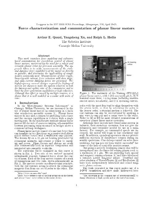
The particular forcer examined in this paper is
shown in Fig. 1. Two sets of two motors 2 mounted
orthogonally generate balanced forces about the center
of mass. Each of the four motors consists of a stack
of laminations and two coils, shown schematically in
Fig. 2. The motors operate on a ux-steering principle,
with the coil currents acting to switch the permanent
magnetic ux from one set of poles to the other. The
1 http://www.cs.cmu.edu/ msl
2 Here, motor refers to one of the four actuators on the forcer,
and planar linear motor refers to the entire device.
The Robotics Institute
Carnegie Mellon University
1
Figure 1: The underside of the Normag 4XY1302-2
planar linear motor, with 1.016 mm tooth pitch, 26 N
nominal static force, 1.8 Kg mass (including interferometer
optics, not shown), and 2 A operating current.
poles with the most ux tend to align themselves with
the platen teeth, so that by activating the poles in
the proper order, a stepping motion is achieved. The
coil currents can also be microstepped by applying a
sine wave to one coil and a cosine wave to the other.
Refer to [2] or [3] for more detailed presentations of
open-loop planar linear motor operation.
Although these motors have found some success in
industry, their open-loop operation does not give the
robustness and versatility needed for use in a minifactory.
For example, as commanded speeds are increased,
the motor will begin to lose synchrony and
stall. In addition, open-loop operation can not provide
su cient rejection of disturbance torques during assembly
operations. Closed-loop control can solve these
problems, but has not yet been widely successful 3 because
of the lack of a suitable position sensor.
Our group is actively developing sensors that will be
incorporated into the forcer for sensing platen teeth to
a resolution of 1 m. We are exploring both optical
and magnetic sensing schemes [4], and have fabricated
a compact 3-DOF magnetic sensor. Crawford and
other students of Youcef-Toumi [5] and Ish-Shalom [6]
have both independently fabricated and tested magnetic
platen sensors.
The work presented in this paper makes use of a
2-DOF (translation and skew angle) high-speed laser
3 The exception is the common use of accelerometers[3] to
damp vibrations at high speeds and at the end of motions.

Figure 2: Basic linear motor operation: Current in the
motor coils generates magnetic ux (dark ux path)
that sums with the permanent magnet ux (light ux
path) to produce forces.
interferometer as a position sensor. Whereas this sensor
has better bandwidth and precision than a platen
tooth sensor, the work presented in this paper is independent
of the particular sensor used, provided it
meets the minimum bandwidth and resolution requirements.
This work is also independent of the higher
level closed-loop control method used for controlling
the forcer.
2 Motor Commutation
In the context of planar linear motors, a commutator
is simply a mechanism that selects motor currents
to achieve a desired force. The usefulness of a commutator
is in providing higher level controllers with
an ideal force source (within actuator limits), as opposed
to a system where a current must be speci ed for
each coil. Commutators separated from higher level
controllers are especially important for planar linear
motors because currents must be commanded at KHz
rates. For example, to operate the planar linear motor
of Fig. 1 at 1 m/s, a sine wave of nearly 1 KHz must
be applied to the motor coils, calling for updates of at
least 2 KHz.
Typically, the forcers are assumed to generate forces
according to the relation:
F gen = ki a sin( )+ki b cos( ); (1)
where F gen is the total force generated by the x-axis
motor pair, k is a constant with units of force over
current, i is the current in coil , and is the phase
of the motor. The phase is de ned as the position of
the motor relative to the nearest tooth pitch, expressed
as an angle:
= 2 x= ; (2)
where is the tooth pitch. This force expression assumes
no manufacturing errors, no magnetic saturation,
uniform teeth, perfect ampli ers, in nite update
rates, and no rotation of the forcer. An identical equation
applies to the y-axis motor pair.
It is convenient to re-parameterize the input currents
according to:
i a = i cos( ) and i b = ,i sin( ); (3)
2
Figure 3: Test setup for static force measurements.
where i and are the new parameters. Combining (1)
and (3) and simplifying yields:
F gen = ki sin( , ): (4)
For open-loop control, force is not usually controlled,
but rather the equilibrium position of the motor.
Typically, i is kept constant at the maximum
value, and a value of = des is used to shift the
equilibrium position of the motor to des.
For closed-loop control, a xed amplitude commutator
can be designed that also keeps i at its maximum
value. However, is now varied to generate forces
by setting it to = , arcsin(F des=ki). This commutation
scheme requires large currents to be in the
motor coils at all times, resulting in unwanted thermal
e ects, but also a potentially useful passive sti ness.
Alternatively, the other input parameter, , can
be xed relative to the motor position so that the
motor is always operating at the peak of the sti ness
curve by setting = , =2. In this approach, force
is controlled by varying the amplitude i according to
i = F des=k. This xed phase commutator will have
reduced thermal e ects, but no passive sti ness.
In the following sections, static and dynamics tests
are performed to determine whether the assumptions
made for (1) are valid.
3 Static Force Characterization
Static force measurements are performed using a
locked rotor test commonly used in motor modeling.
In this test, a constant set of currents is applied to the
motor coils. A load is applied to the motor through
a force gauge, and the force is recorded as the motor
de ects from its equilibrium position. The test setup
is shown in Fig. 3.
The locked rotor test is slightly more complicated
for planar linear motors because their air bearings allow
for 3 DOFs. An external constraint or rotation
servo is required to keep the forcer from rotating. As
an external constraint would be di cult to align, the y
motors of the forcer are used to regulate the skew angle
to zero. A PID angle controller with a xed-amplitude
commutator is used for skew angle regulation and passive
sti ness in the (unsensed) y direction.

force [N]
40
30
20
10
0
−10
−20
−30
−40
0 0.2 0.4 0.6 0.8 1 1.2 1.4 1.6 1.8 2
position [mm]
Figure 4: Force versus position ( ), measured data ( )
di er from a sine function (solid line) by a small error
(dashed line). Here, =0 and i = 2A.
3.1 Experimental setup
The experimental setup, shown in Fig. 3, consists
of a Normag forcer on a Normag platen connected
through a double universal joint linkage to an Entran
load cell. The load cell is mounted on a 3-axis micrometer
stage, with the x translation controlled by
a Newport automated micrometer. The coupling between
the forcer and load cell is designed to transmit
only axial forces, and to attach to the forcer as low as
possible, to minimize torques that may tend to de ect
the air bearing. As there is signi cant compliance in
this coupling, a Zygo two-axis high-speed interferometer
is used to monitor the true position and skew angle
of the forcer.
For these tests, the currents in the x motors of the
forcer are set to xed values using (3). After setting
these currents, there is a delay of10minutes to minimize
thermal expansions during data collection. Next,
the micrometer is commanded to move in short increments
over a range of two pitch units. After the
micrometer settles to each commanded position, the
load cell and interferometer are read and the values
stored. The force generated by the forcer as a function
of position is shown in the sti ness curve of Fig.
4. This test is repeated with di erent values of parameters
and i in (3). The data collection procedure is
fully automated, allowing more data to be collected
than would otherwise be feasible.
3.2 Experimental results
A total of 127 tests were completed to generate sti -
ness curves for from 0 to 180 , and for i from -2.0 A
to 2.0 A. For each run, the micrometer was positioned
every 25 m along a 2032 m (2 pitch) distance. The
total data collection time was about 32 hours, taken
over several days.
Fig. 4 shows a typical sti ness curve. Note that
the sine function matches the data points 4 to within
1.5 N. Also note that, neglecting higher harmonics, it is
only the amplitude of the sine function which is useful,
because the phase and period of the sine function are
determined by the tooth pitch and the phase .Thus,
only the peaks of the sti ness curves can be plotted for
multiple runs on one diagram, as in Fig. 5. This gure
4 The points are not evenly spaced due to compliance in the
force linkage.
3
force amplitude [N]
40
30
20
10
0
−10
−20
−30
0.00 A
−40
0 22.5 45 67.5 90 112.5 135 157.5 180
commutation phase (degrees)
2.00 A
1.50 A
1.25 A
1.00 A
0.75 A
0.50 A
0.25 A
−0.25 A
−0.50 A
−0.75 A
−1.00 A
−1.25 A
−1.50 A
−2.00 A
Figure 5: Force ripple, showing the peak force capability
of the forcer as a function of input parameters
and i.
Peak force [N]
30
20
10
0
−10
−20
−30
−2 −1.5 −1 −0.5 0 0.5 1 1.5 2
Current in coil A [amps]
Figure 6: Force linearity, showing peak force as a function
of i, with =0. Measured values (+), and Eq. (5)
t to these data (solid line).
shows the variation of the peak force of the forcer as
the parameters i and vary.
This plot shows signi cant force ripple when the
motor is commutated with (3), exceeding 20% in
places. If smoother force generation is desired, these
data can be used to correct the motor forces. One
approach is to generate a lookup table that gives an
appropriate set of currents as a function of the phase
angle and desired force, as in [7]. However, this technique
requires a complete set of force data to generate
the lookup table for each forcer. While three days of
data collection to get these data once is reasonable, it
seems excessive to do this for each forcer needed in a
minifactory.
Fortunately, wemay be able to use a simpler technique.
Plotting a vertical cross section of the data for
=0 produces Fig. 6. This curve should be close to
linear if (1) is valid. However, there is signi cant deviation
from linearity due to magnetic saturation. This
nonlinear function is well modeled by a simple function
such as 5 :
f c = a0i c , a1 ji cj i c; (5)
where i c is the current applied to the motor coil, f c
is the peak force generated by the coil, and a0 and a1
5 Chai and Leenhouts[8] have used similar empirical functions
to model the saturation in rotary stepper motors.

Peak force [N]
40
35
30
25
20
−1 −0.8 −0.6 −0.4 −0.2 0 0.2 0.4 0.6 0.8 1
Skew angle [degrees]
Figure 7: Peak force as a function of forcer skew angle,
with i=2 A and 1;2 =0 (solid line) or 1;2 =45
(dashed line).
are positive parameters that must be determined for
each motor coil. The curve connecting the data points
in Fig. 6 is generated by computing the a0 and a1
parameters based only on the slope of the data at zero
current and the magnitudes at maximum currents. In
contrast to a 3D lookup table, the data needed to t
this curve can be taken in a manner of minutes using a
hand-held force gauge for a pull-out test to determine
the peak forces for only four values of i. Early results
indicate that the magnetic saturation e ect accounts
for slightly more than half of the force ripple. The
remaining ripple is probably due to higher order terms
in the sti ness curves.
Force generated by the forcers is also dependent on
the skew angle. As the forcer rotates slightly, the long
motor teeth only partially overlap the platen teeth,
causing the peak force to decrease. At large rotations,
the forcers can not operate, but they can be used as
a ne-motion device with a motion range of a few degrees.
To allow control of the motor skew angle, it must
be included in Eq. (1). The misalignment of teeth will
cause a decrease in k with increasing angle magnitude,
and the phases of the two motors mounted on opposite
sides of the forcer will shift in opposite directions
as the angle changes. Thus, Eq. (1) and Eq. (2) are
replaced by:
F gen = k( )i a1 sin( 1)+k( )i b1 cos( 1)
+k( )i a2 sin( 2)+k( )i b2 cos( 2); (6)
1 = x + ; 2 = x , ; (7)
where x is given by (2). The e ect of on the phase
position of each motor is re ected in the term =
l 2 = , where, is the forcer skew angle, and l is
half the distance between each pair of motors. Note
that four current values per axis are needed to control
the forcer rotation, so that (3) is replaced by:
i a1 = i cos( 1 + ); i b1 = ,i sin( 1 + );
i a2 = i cos( 2 , ); i b2 = ,i sin( 2 , ):(8)
These equations will feed-forward the appropriate
phase to each motor based on the rotation angle. However,
the function k( ) is still unknown. To examine
this function, the locked rotor test is repeated, using
the y motors to servo the forcer skew angle to nonzero
values. The data in Fig. 7 show a force dropo
with increasing angle magnitude, as expected. Each
plot also shows an artifact from the uncompensated
force ripple, because as changes, the arguments of
the transcendentals in (8) will change. Thus, the ripple
shown as varies in Fig. 5 also appears here.
4
Figure 8: System latencies and control rates cause the
motor's output force to drop at high velocities.
4 Dynamic measurements
The importance of dynamic e ects was evident in
initial closed-loop control experiments using the xed
phase commutator described in Sec. 2. While our
open-loop controllers were able to drive motors to velocities
over 1 m/s, motors under closed-loop control
could not reach even half that speed. As discussed below,
the reason for this limitation is delays in the commutator,
which can be corrected by adding a phase
advance term to the forcer position.
Another signi cant dynamic e ect is the eddy current
damping force caused by the large time-varying
magnetic elds generated as the motor passes over the
unlaminated steel platen surface. As these forces act in
opposition to the forcer velocity, they are often treated
as a mechanical damping e ect [9]. As shown below,
these forces can be measured by examining the acceleration
responses resulting from bidirectional step force
commands.
4.1 Phase advance
The initial closed-loop controller does not perform
as well as the open-loop controller because the feedback
loop contains delays, making the motor position
sensed at the beginning of the closed-loop cycle invalid
by the time the output is produced. Fig. 8 shows this
e ect in more detail. The sti ness curve shown assumes
the motor is at the location read by the sensor.
The goal is to set the motor currents so that the motor
is operating at the peak of the sti ness curve, shown
as a star. However, while the sensor signal is being
processed and new outputs take e ect, the motor will
have moved, causing the output to miss the peak of
the sti ness curve by an amount v t l, the velocity of
the motor times the latency. In addition, since the
updates occur at discrete times, the motor force over
the next output cycle will span a range of the sti ness
curve of length v=r, where v is the motor velocity and
r is the output update rate in Hz. So instead of getting
the commanded force (the star), we get a reduced
force that changes during the output interval (the bold
arrow). By using a phase advance term of vt l + v
2r we
can shift the bold arrow so that it is centered about
the peak of the sti ness curve 6 . The approach isto
determine the latency time and commutation rate of
6 Note that the average force will always be lower than the
peak for nite commutation rates, and that with xed commutation
rates, this e ect will cause the available force to decrease
with velocity.

Average Acceleration [m/s^2]
18
16
14
12
10
300 350 400 450 500 550 600 650 700
Phase advance time [usecs]
Figure 9: Average acceleration as a function of the
phase advance time. The computed value is indicated
by the vertical dashed line.
the commutator and compute a delay time (in units
of seconds). This value is multiplied by the latest velocity
to get a phase advance position o set, which is
added to the latest position. The sum is the expected
motor position when the output takes e ect.
Commutator latencies include input and output delays
and computation times. For our system, the input
delay is negligible. The commutation code running on
a Motorola 68040 takes 200 s to compute output currents
based on the input position.
The ampli ers introduce an output delay which is
slightly more complicated to measure. To do so, a
spectrum analyzer is used to measure the transfer function
of the ampli er driving one motor of a stationary
forcer oating on the platen. Note that the ampli er
dynamics can be reasonably modeled by a constant
delay time as long as the lowest frequency poles and
zeros are above the driving frequencies of interest. If
this is not the case, the delay time will have tovary
with the commanded velocity. For our ampli er, the
lowest pole appears to be at 1400 Hz, yielding a constant
delay time of 114 s.
The last delay is from the commutation update rate,
3500 Hz for these tests, giving a total delay time of
1
2
1
+ 114 + 200 = 457 s:
3500
This value is the delay time that is multiplied by the
motor velocity to compute the amount of phase advance.
4.2 Experimental veri cation
Tovalidate the estimated phase advance delay time,
full scale force commands are sent to a xed phase
commutator controlling the x motors of the forcer for
a range of values for the phase advance delay time.
As with the static force measurements, a PID controller
with a xed amplitude commutator controlling
the y motors is used to prevent both skew angles and
y translations. Force commands are generated such
that the motor will accelerate forward and backwards
at maximum acceleration between velocities of -1 m/s
and 1 m/s several times 7 . The complete sequence typically
takes less than 0.5 s, with motions of under 50
mm.
The interferometer position data for the two long
constant acceleration segments are di erenced to get
velocity. Over repeated runs with varying phase advance
delay times, the fastest response indicates the
best value for the delay time. To quantify the fastest
response, a velocity of 1.6 m/s is divided by the time
7 While the forcer can move as fast as 2 m/s, the interferometer
has a limit of 1 m/s.
5
Position [m]
Velocity [m/s]
0.03
0.025
0.02
0.015
0.01
0.005
0
0 0.01 0.02 0.03
Time [seconds]
0.04 0.05 0.06
1
0.8
0.6
0.4
0.2
0
0 0.01 0.02 0.03
Time [seconds]
0.04 0.05 0.06
Figure 10: Trajectory (solid line) tracking with
(dashed line) and without (dotted line) phase advance.
it takes for the forcer to change from +0.8 m/s to -0.8
m/s, to compute an average acceleration.
Fig. 9 shows this average acceleration as a function
of the phase advance time. Note that the peak force
matches the phase advance time computed in the previous
section to within 50 s.
To demonstrate the improvement from the phase
advance term, Fig. 10 shows the position and velocity
trajectories for a peak acceleration command starting
from a rest position. Note that although adding phase
advance yields a substantial improvement, it is still
not as fast as the theoretical maximum because of decreased
forces from nite control rates and eddy current
damping forces, discussed below.
It should be noted that phase advance is a common
technique used in the control of stepper motors. It
has even been previously applied to linear and planar
motors [5, 10]. However, these works do not give much
intuition on computing the phase advance functions.
4.3 Eddy current damping forces
To measure the eddy current damping force, rst
note that this force is always opposite in sign to the
motor velocity. Thus, it increases the e ective maximum
actuator forces during decelerations, and decreases
them during accelerations.
Using the proper value for the phase advance parameter,
the bang-bang acceleration tests of the previous
section are repeated. This time, the interferometer
position data are di erenced twice to get an acceleration
signal, and ltered to reduce the noise from force
ripple and other sources. The motor acceleration as a
function of velocity for the two constant acceleration
segments of the motor trajectory can then be plotted.
The upper traces in Fig. 11 show ten repeated runs as
well as an average for the positive acceleration segment
of the trajectory. The lower traces show the same for
the negative acceleration segment of the trajectory.
The eddy current damping force as a function of
velocity is computed by averaging the upper and
lower curves. This computation gives the acceleration
change caused by the eddy currents, which can
be multiplied by the motor mass, 1.8 Kg, to get the
eddy current damping force. This result is shown in
the middle trace of Fig. 11.
Although these data are rather noisy, they appear

Force [N]
40
30
20
10
0
−10
−20
−30
−40
Acceleration [m/s*s]
25
20
15
10
5
0
−5
−10
−15
−20
−25
−1 −0.6 −0.5 −0.4 −0.2 0 0 0.5
Velocity [m/s]
0.2 1 0.4 0.6
Figure 11: Acceleration and eddy current forces versus
velocity. The upper and lower traces show acceleration
vs. velocity. The middle trace shows the damping
force. The dashed straight line is the damping force
linearized about zero velocity
to show that the eddy current damping forces are not
linear, but level o after a velocity of about 0.5 m/s.
Ongoing work includes the use of an accelerometer and
additional runs to produce a less noisy version of Fig.
11 that can be used to predict the eddy current forces
at high velocities. This information is necessary to
characterize the acceleration limits of the forcer for
use by trajectory planners.
Nordquist and Smith [11] use an alternate method
for computing the eddy current damping forces. They
assume the motor can be modeled over small displacements
from an equilibrium position as a linear springmass-damper
system. An impulse response test is used
to determine the damping ratio of the system based
on the motor mass and local sti ness. Applying this
method to the Normag forcer gives a damping coe -
cient, k v, of 37.2 N/m/s. The resulting linear damping
force curve from this damping coe cientisshown plotted
as a dashed line in Fig. 11, which seems to match
the slope of our eddy current force computation only
near zero velocity. However, this estimate supports the
conclusion of a non-linear eddy-current force, because
if this line is extended to higher velocities, it will cause
drastic drops in the available acceleration, which are
not observed here.
Gjeltema [2], using a Normag motor, found the eddy
current drag forces to be linear with velocity. However,
only the acceleration characteristics of the motor
are examined. Without deceleration data, damping
forces (which decrease the maximum acceleration and
increase the maximum deceleration) can not be distinguished
from ampli er dynamics and commutation
update rate e ects (which decrease the maximum acceleration
and deceleration).
5 Conclusions
In summary, static and dynamic force measurements
of planar linear motors have been presented that
support the following conclusions:
The sti ness curve of the motor is reasonably approximated
by a sine function.
6
The amplitude of this sine function is a non-linear
function of current.
The available force of the forcer decreases with
skew angle, falling to 50% at about 1:0 .
A phase advance term is necessary to overcome
commutator latency and update rate delay times,
and can be measured by determining the time between
sensor reads and output updates.
Eddy current damping forces are non-linear and
can be computed by averaging positive and negative
acceleration curves at each velocity value.
This work provides the foundation for an integrated
forcer/sensor under development. This platform will
be used for evaluating a number of high-performance
control strategies needed for application areas including
precision assembly in a minifactory system.
Acknowledgements
This work is supported in part by NSF grants DMI-
9523156 and DMI-9527190, and the CMU Engineering
Design Research Center. Quaid is supported by an
AT&T Fellowship. We thank IBM for the donation
of the planar linear motor and interferometer systems,
and Al Rizzi, Zack Butler, and Pat Muir for helpful
discussions.
References
[1] A. A. Rizzi, J. Gowdy, and R. L. Hollis, \Agile assembly architecture:
An agent based approach to modular precision
assembly systems," in Proc. IEEE Int. Conf. Robt. Aut.,
April 1997.
[2] P. D. Gjeltema, \The design of a closed loop linear motor
system," Master's thesis, MIT, June 1993.
[3] E. R. Pelta, \Precise positioning without geartrains," Machine
Design, pp. 79{83, April 1987.
[4] A. E. Brennemann and R. L. Hollis, \Magnetic and opticaluorescence
position sensing for planar linear motors," in
Proc. Int'l Conf. on Intelligent Robots and Systems, vol. 3,
pp. 101{107, August 1995.
[5] D. S. Crawford, \Sensor design and feedback motor control
for two dimensional linear motors," Master's thesis, MIT,
May 1995.
[6] J. Ish-Shalom, \Sub-micron large motion multi-robot planar
motion system," in 7th ISRR Conference, 1995.
[7] P. F. Muir, \Converting a commercial electric direct-drive
robot to operate from joint torque commands," Tech.
Rep. SAND91-1548, UC-408, Sandia National Laboratories,
1991.
[8] H. D. Chai and A. C. Leenhouts, \Position error analysis
for microstepping," in Proceedings of the Fourteenth Annual
Symposium on Incremental Motion Control Systems
and Devices, pp. 265{274, 1985.
[9] W. E. Hinds and B. Nocito, \15: The sawyer linear motor,"
in Theory and Application of Step Motors (B. Kuo, ed.),
pp. 327{340, St. Paul, West Publishing Co., 1974.
[10] J. Ish-Shalom, \Experimental results of using a step motor
as a spring," in Proc. IEEE Int'l Conf. on Robotics and
Automation, pp. 1841{1846, May 1989.
[11] J. I. Nordquist and P. M. Smit, \A motion-control system
for (linear) stepper motors," in Proceedings of the Fourteenth
Annual Symposium on Incremental Motion Control
Systems and Devices, pp. 215{231, 1985.