Errors for Linear Systems When we solve a - TerpConnect
Errors for Linear Systems When we solve a - TerpConnect
Errors for Linear Systems When we solve a - TerpConnect

Create successful ePaper yourself
Turn your PDF publications into a flip-book with our unique Google optimized e-Paper software.
<strong>Errors</strong> <strong>for</strong> <strong>Linear</strong> <strong>Systems</strong><br />
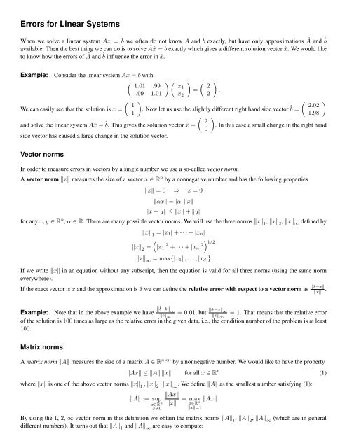
<strong>When</strong> <strong>we</strong> <strong>solve</strong> a linear system Ax = b <strong>we</strong> often do not know A and b exactly, but have only approximations  and ˆ b<br />
available. Then the best thing <strong>we</strong> can do is to <strong>solve</strong> ˆx = ˆ b exactly which gives a different solution vector ˆx. We would like<br />
to know how the errors of  and ˆ b influence the error in ˆx.<br />
Example: Consider the linear system Ax = b with<br />
<br />
1.01 .99 x1 2<br />
= .<br />
.99 1.01 x2 2<br />
<br />
1<br />
We can easily see that the solution is x = . Now let us use the slightly different right hand side vector<br />
1<br />
ˆ <br />
2.02<br />
b =<br />
1.98<br />
and <strong>solve</strong> the linear system Aˆx = ˆ <br />
2<br />
b. This gives the solution vector ˆx = . In this case a small change in the right hand<br />
0<br />
side vector has caused a large change in the solution vector.<br />
Vector norms<br />
In order to measure errors in vectors by a single number <strong>we</strong> use a so-called vector norm.<br />
A vector norm x measures the size of a vector x ∈ R n by a nonnegative number and has the following properties<br />
x = 0 ⇒ x = 0<br />
αx = |α| x<br />
x + y ≤ x + y<br />
<strong>for</strong> any x, y ∈ R n , α ∈ R. There are many possible vector norms. We will use the three norms x 1 , x 2 , x ∞ defined by<br />
x1 = |x1| + · · · + |xn|<br />
<br />
x2 = |x1| 2 + · · · + |xn| 2 1/2<br />
x ∞ = max{|x1| , . . . , |xd|}<br />
If <strong>we</strong> write x in an equation without any subscript, then the equation is valid <strong>for</strong> all three norms (using the same norm<br />
everywhere).<br />
If the exact vector is x and the approximation is ˆx <strong>we</strong> can define the relative error with respect to a vector norm as ˆx−x<br />
x .<br />
Example: Note that in the above example <strong>we</strong> have ˆ b−b ∞<br />
b ∞<br />
= 0.01, but ˆx−x ∞<br />
x ∞<br />
= 1. That means that the relative error<br />
of the solution is 100 times as large as the relative error in the given data, i.e., the condition number of the problem is at least<br />
100.<br />
Matrix norms<br />
A matrix norm A measures the size of a matrix A ∈ R n×n by a nonnegative number. We would like to have the property<br />
Ax ≤ A x <strong>for</strong> all x ∈ R n<br />
where x is one of the above vector norms x 1 , x 2 , x ∞ . We define A as the smallest number satisfying (1):<br />
A := sup<br />
x∈Rn Ax<br />
x<br />
x=0<br />
= max<br />
x∈Rn Ax<br />
x=1<br />
By using the 1, 2, ∞ vector norm in this definition <strong>we</strong> obtain the matrix norms A 1 , A 2 , A ∞ (which are in general<br />
different numbers). It turns out that A 1 and A ∞ are easy to compute:<br />
(1)
Theorem:<br />
A ∞ = max<br />
A 1 = max<br />
<br />
i=1,...,n<br />
j=1,...,n<br />
<br />
j=1,...,n<br />
i=1,...,n<br />
Proof: For the infinity norm <strong>we</strong> have<br />
|aij| (maximum of row sums of absolute values)<br />
|aij| (maximum of column sums of absolute values)<br />
Ax ∞ = max<br />
i<br />
<br />
<br />
<br />
<br />
<br />
<br />
implying A∞ ≤ maxi <br />
and Ax∞ = maxi j |aij|.<br />
For the 1-norm <strong>we</strong> have<br />
Ax1 = <br />
<br />
<br />
<br />
<br />
<br />
<br />
j<br />
aijxj<br />
<br />
⎛<br />
<br />
<br />
<br />
<br />
≤ max |aij| |xj| ≤ ⎝max<br />
i<br />
i<br />
j<br />
j<br />
|aij|<br />
⎞<br />
⎠ x ∞<br />
<br />
j |aij|. Let i∗ be the index where the maximum occurs and define xj = sign ai∗j, then x ∞ = 1<br />
i<br />
j<br />
aijxj<br />
<br />
<br />
<br />
<br />
≤<br />
<br />
j<br />
i<br />
|aij|<br />
<br />
|xj| ≤<br />
<br />
implying A1 ≤ maxj i |aij|. Let j∗ be the index where the maximum occurs and define xj∗ = 1 and xj <br />
= 0 <strong>for</strong> j = j∗,<br />
then x1 = 1 and Ax1 = maxj i |aij|. <br />
<br />
max<br />
j<br />
We will not use A 2 since it is more complicated to compute (it involves eigenvalues).<br />
Note that <strong>for</strong> A, B ∈ R n×n <strong>we</strong> have AB ≤ A B since<br />
The following results about matrix norms will be useful later:<br />
ABx ≤ A Bx = A B x .<br />
Lemma 1: Let A ∈ Rn×n be nonsingular and E ∈ Rn×n . Then E < 1<br />
A−1 implies that A + E is nonsingular.<br />
<br />
Proof: Assume that A + E is singular. Then there exists a nonzero x ∈ Rn such that (A + E)x = 0 and hence<br />
x<br />
A−1 ≤ Ax = Ex ≤ E x<br />
<br />
The left inequality <strong>for</strong> b := Ax follows from x = <br />
A−1b ≤ A−1 1<br />
b. As x > 0 <strong>we</strong> obtain A−1 ≤ E.<br />
<br />
Lemma 2: For given vectors x, y ∈ R n with x = 0 there exists a matrix E ∈ R n×n with Ex = y and E = y<br />
x .<br />
Proof: For the infinity-norm <strong>we</strong> have x ∞ = |xj| <strong>for</strong> some j. Let a ∈ R n be the vector with aj = 1, ak = 0 <strong>for</strong> j = k and<br />
let<br />
E = 1<br />
x ya⊤ ,<br />
then (i) a ⊤ x = x ∞ implies Ex = y and (ii) ya ⊤ v ∞ = a ⊤ v y∞ with a ⊤ v ≤ v∞ implies E ≤ y<br />
x .<br />
For the 1-norm <strong>we</strong> use a ∈ R n with aj = sign(xj) since a ⊤ x = x 1 and a ⊤ v ≤ v1 .<br />
For the 2-norm <strong>we</strong> use a = x/ x 2 since a ⊤ x = x 2 and a ⊤ v ≤ a2 v 2 = v 2 .<br />
Condition numbers<br />
Let x denote the solution vector of the linear sytem Ax = b. If <strong>we</strong> choose a slightly different right hand side vector ˆb then<br />
<strong>we</strong> obtain a different solution vector ˆx satisfying Aˆx = ˆ <br />
<br />
b. We want to know how the relative error ˆ <br />
<br />
b − b<br />
/ b influences<br />
the relative error ˆx − x / x (“error propagation”). We have A(ˆx − x) = ˆb − b and there<strong>for</strong>e<br />
<br />
<br />
ˆx − x = A −1 ( ˆ <br />
<br />
b − b) ≤ −1<br />
A <br />
<br />
ˆ <br />
b − b<br />
.<br />
<br />
i<br />
|aij|<br />
<br />
x 1
On the other hand <strong>we</strong> have b = Ax ≤ A x. Combining this <strong>we</strong> obtain<br />
ˆx − x<br />
x ≤ A −1<br />
A <br />
<br />
<br />
<br />
ˆ <br />
<br />
b − b<br />
b .<br />
The number cond(A) := A A−1 is called condition number of the matrix A. It determines how much the relative<br />
error of the right hand side vector<br />
can be amplified. The condition number depends on the choice of the matrix norm: In<br />
general cond1(A) := A <br />
1 A−1 <br />
and cond∞(A) := A <br />
1 ∞ A−1 are different numbers.<br />
∞<br />
Example: In the above example <strong>we</strong> have<br />
<br />
cond∞(A) = A −1<br />
∞ A <br />
<br />
= 1.01<br />
∞ .99<br />
<br />
.99 ∞ <br />
25.25<br />
1.01 −24.75<br />
<br />
−24.75 ∞<br />
= 2 · 50 = 100<br />
25.25<br />
and there<strong>for</strong>e<br />
ˆx − x<br />
x<br />
<br />
<br />
<br />
≤ 100<br />
ˆ <br />
<br />
b − b<br />
b<br />
which is consistent with our results above (b and ˆ b <strong>we</strong>re chosen so that the worst possible error magnification occurs).<br />
The fact that the matrix A in our example has a large condition number is related to the fact that A is close to the singular<br />
matrix B =<br />
1 1<br />
1 1<br />
<br />
.<br />
The following result shows that<br />
Theorem: min<br />
B∈Rn×n A − B<br />
, B singular<br />
1<br />
cond(A) indicates how close A is to a singular matrix:<br />
A =<br />
1<br />
cond(A)<br />
Proof: (1) Lemma 1 shows: B singular implies A − B ≥ 1<br />
A −1 .<br />
(2) By the definition of A −1 there exist x, y ∈ R n such that x = A −1 y and A −1 = x<br />
y<br />
matrix E ∈ R n×n such that Ex = y and E = y<br />
x<br />
singular and A − B = E = 1<br />
A−1 . <br />
. By Lemma 2 there exists a<br />
. Then B := A − E satisfies Bx = Ax − Ex = y − y = 0, hence B is<br />
Example:<br />
<br />
1.01<br />
The matrix A =<br />
.99<br />
<br />
<br />
.99<br />
1<br />
is close to the singular matrix B =<br />
1.01<br />
1<br />
<br />
1<br />
so that<br />
1<br />
A−B∞ A =<br />
∞<br />
.02<br />
2 = .01.<br />
1<br />
By the theorem <strong>we</strong> have that 0.01 ≤ cond∞(A) or cond∞(A) ≥ 100. As <strong>we</strong> say above <strong>we</strong> have cond∞(A) = 100, i.e., the<br />
matrix B is really the closest singular matrix to the matrix A.<br />
<strong>When</strong> <strong>we</strong> <strong>solve</strong> a linear system Ax = b <strong>we</strong> have to store the entries of A and b in the computer, yielding a matrix  with<br />
rounded entries âij = fl(aij) and a rounded right hand side vector ˆb. If the original matrix A is singular then the linear<br />
system has no solution or infinitely many solutions, so that any computed solution is meaningless. How can <strong>we</strong> recognize<br />
this on a computer? Note that the matrix  which the computer uses may no longer be singular.<br />
1<br />
Ans<strong>we</strong>r: We should compute (or at least estimate) cond( Â). If cond(Â) < then <strong>we</strong> can guarantee that any matrix A<br />
εM<br />
which is rounded to  must be nonsingular: |âij<br />
<br />
<br />
− aij| ≤ εM |aij| implies  − A<br />
≤ εM A <strong>for</strong> the infinity or 1-norm.<br />
There<strong>for</strong>e Â−A<br />
 ≤<br />
εM<br />
1−εM ≈ εM<br />
1−εM<br />
and cond( Â) < εM<br />
nonsingular by the theorem.<br />
≈ 1<br />
εM<br />
Now <strong>we</strong> assume that <strong>we</strong> perturb both the right hand side vector b and the matrix A:<br />
Â−A<br />
imply<br />
 < 1 . Hence the matrix A must be<br />
cond( Â)
Theorem: Assume Ax = b and ˆx = ˆ <br />
<br />
b. If A is nonsingular and  − A<br />
≤ 1/ A−1 there holds<br />
ˆx − x<br />
x ≤<br />
cond(A)<br />
1 − cond(A) Â−A<br />
⎛<br />
<br />
<br />
⎝<br />
A<br />
ˆ <br />
<br />
b − b<br />
b +<br />
<br />
<br />
⎞<br />
 − A<br />
⎠<br />
A<br />
Proof: Let E = Â − A, hence Aˆx = ˆb − Eˆx. Subtracting Ax = b gives A(ˆx − x) = ( ˆb − b) − Eˆx and there<strong>for</strong>e<br />
ˆx − x ≤ −1<br />
A <br />
<br />
ˆ <br />
b − b<br />
+ E ˆx .<br />
Dividing by x and using b ≤ A x ⇐⇒ x ≥ b / A gives<br />
ˆx − x<br />
x ≤ −1<br />
A ⎛<br />
<br />
<br />
A ⎝<br />
ˆ <br />
<br />
⎞<br />
b − b<br />
E ˆx<br />
+ ⎠<br />
b A x<br />
Now <strong>we</strong> have ˆx<br />
x<br />
assertion. <br />
If cond(A) Â−A<br />
A<br />
If cond(A) Â−A<br />
A<br />
≤ x+ˆx−x<br />
x<br />
= 1 + ˆx−x<br />
ˆx−x<br />
x . By putting x<br />
on the left hand side and solving <strong>for</strong> it <strong>we</strong> obtain the<br />
≪ 1 <strong>we</strong> have that both the relative error in the right hand side vector and in the matrix are magnified by<br />
cond(A).<br />
= A−1 <br />
<br />
 − A<br />
≥ 1 then by the theorem <strong>for</strong> the condition number the matrix  may actually be<br />
singular, so that the solution ˆx is no longer <strong>we</strong>ll defined.<br />
Computing the condition number<br />
We have seen that the condition number is very useful: It tells us what accuracy <strong>we</strong> can expect <strong>for</strong> the solution, and how<br />
close our matrix is to a singular matrix.<br />
In order to compute the condition number <strong>we</strong> have to find A −1 . This takes n 3 +O(n 2 ) operations, compared with n3<br />
3 +O(n2 )<br />
operations <strong>for</strong> the LU-decomposition. There<strong>for</strong>e the computation of the condition number would make the solution of a linear<br />
system 3 times as expensive. For large problems this is not reasonable.<br />
Ho<strong>we</strong>ver, <strong>we</strong> do not need to compute the condition number with full machine accuracy. Just knowing the order of magnitude<br />
is sufficient. Assume that <strong>we</strong> pick a vector c and <strong>solve</strong> the linear sytem Az = c. Then z = A −1 c and z ≤ A −1 c or<br />
<br />
A −1 ≥ z<br />
c .<br />
This gives us a lo<strong>we</strong>r bound <strong>for</strong> A −1 , and the cost of this operation is only n 2 + O(n). The trick is to pick c such that z<br />
c<br />
becomes as large as possible, so that the lo<strong>we</strong>r bound is close A −1 . There are a number of heuristic methods available<br />
which achieve fairly good lo<strong>we</strong>r bounds: (i) Pick c = (±1, . . . , ±1) and pick the signs so that the <strong>for</strong>ward susbstitution gives<br />
a large vector, (ii) picking ˜c := z and <strong>solve</strong> A˜z = ˜c often improves the lo<strong>we</strong>r bound. The Matlab functions condest(A)<br />
and 1/rcond(A) use similar ideas to give lo<strong>we</strong>r bounds <strong>for</strong> cond1(A). Typically they give an estimated condition number<br />
c with c ≤ cond1(A) ≤ 3c and require the solution of 2 or 3 linear systems which costs O(n 2 ) operations if the LU<br />
decomposition is known. (Ho<strong>we</strong>ver, the Matlab commands condest and rcond only use the matrix A as an input value,<br />
so they have to compute the LU decomposition of A first and need n3<br />
3 + O(n2 ) operations.)<br />
Computation in machine arithmetic and residuals<br />
<strong>When</strong> <strong>we</strong> run Gaussian elimination on a computer each single operation causes some roundoff error, and instead of the exact<br />
solution x of a linear system <strong>we</strong> only get an approximation ˆx. As explained above <strong>we</strong> should select the pivot candidate with<br />
the largest absolute value to avoid unnecessary subtractive cancellation, and this usually is a numerically stable algorithm.<br />
Ho<strong>we</strong>ver, there is no theorem which guarantees this <strong>for</strong> partial pivoting (row interchanges). (For “full pivoting” with row<br />
and column interchanges some theoretical results exist. Ho<strong>we</strong>ver, this algorithm is more expensive, and <strong>for</strong> all practical<br />
examples partial pivoting seems to work fine.)
Question 1: How much error do <strong>we</strong> have to accept <strong>for</strong> ˆx−x<br />
x ? This is the unavoidable error which occurs even <strong>for</strong> an<br />
ideal algorithm where <strong>we</strong> only round the input values and the output value to machine accuracy, and use infinite accuracy<br />
<strong>for</strong> all computations.<br />
<strong>When</strong> <strong>we</strong> want to <strong>solve</strong> Ax = b <strong>we</strong> have to store the entries of A, b in the computer, yielding a matrix  and a right hand<br />
side vector ˆ b of machine numbers so that Â−A<br />
A<br />
linear system exactly, i.e., compute a vector ˆx such that ˆx = ˆ b. Then <strong>we</strong> have<br />
ˆx − x<br />
x ≤<br />
≤ εM and ˆ b−b<br />
b ≤ εM. An ideal algorithm would then try to <strong>solve</strong> this<br />
cond(A)<br />
(εM + εM) ≈ 2 cond(A)εM<br />
1 − cond(A)εM<br />
if cond(A) ≪ 1/εM. There<strong>for</strong>e the unavoidable error is 2 cond(A)εM.<br />
Question 2: After <strong>we</strong> computed ˆx how can <strong>we</strong> check how good our computation was? The obvious thing to check is<br />
ˆb := Aˆx and to compare it with b. The difference r = ˆb − b is called the residual. As Ax = b and Aˆx = ˆb <strong>we</strong> have<br />
<br />
<br />
ˆx − x<br />
<br />
≤ cond(A)<br />
x ˆ <br />
<br />
b − b<br />
b<br />
<br />
<br />
where ˆ <br />
<br />
b − b<br />
/ b is called the relative residual. We can compute (or at least estimate) cond(A), and there<strong>for</strong>e can obtain<br />
an upper bound <strong>for</strong> the error ˆx − x / x. Actually, <strong>we</strong> can obtain a slightly better estimate by using<br />
<br />
<br />
ˆx − x = A −1 <br />
ˆ <br />
b − b ≤ A−1 <br />
<br />
<br />
<br />
ˆ ˆx − x<br />
<br />
b − b<br />
=⇒ ≤ cond(A)<br />
ˆx ˆ <br />
<br />
b − b<br />
A ˆx<br />
<br />
<br />
<br />
with the <strong>we</strong>ighted residual ρ :=<br />
ˆ <br />
<br />
b − b<br />
. Note that ˆx − x / ˆx ≤ δ implies <strong>for</strong> δ < 1<br />
A ˆx<br />
ˆx − x ≤ δ x + (ˆx − x) ≤ δ (x + ˆx − x) =⇒<br />
ˆx − x<br />
x<br />
≤ δ<br />
1 − δ<br />
which is the same as δ up to higher order terms O(δ2 ).<br />
<br />
<br />
If ˆ <br />
<br />
b − b<br />
/ b is not much larger than εM then the computation was numerically stable: Just perturbing the input slightly<br />
from b to ˆ b and then doing everything else exactly would give the same result ˆx.<br />
But it can happen that the relative residual is much larger than εM, and yet the computation is numerically stable. We obtain<br />
a better way to measure numerical stability by considering perturbations of the matrix A:<br />
Assume <strong>we</strong> have a computed solution ˆx. If <strong>we</strong> can find a slightly perturbed matrix à such that<br />
<br />
<br />
à − A<br />
≤ ε,<br />
A<br />
Èx = b (2)<br />
where ε not much larger than εM, then the computation is numerically stable: Just perturbing the matrix within the roundoff<br />
error and then doing everything exactly gives the same result as our computation.<br />
How can <strong>we</strong> check whether such a matrix à exists? We again use the “<strong>we</strong>ighted residual”<br />
<br />
<br />
<br />
ρ :=<br />
ˆ <br />
<br />
b − b<br />
A ˆx .<br />
Then:<br />
1. If ˆx is the solution of a slightly perturbed problem (2) <strong>we</strong> have ρ ≤ ε.
2. If ρ ≤ ε then ˆx is the solution of a slightly perturbed problem (2).<br />
Proof:<br />
1. Let E = Ã − A. Then (A + E)ˆx = b or ˆb − b = −Eˆx yielding<br />
<br />
<br />
ˆ <br />
<br />
<br />
<br />
<br />
b − b<br />
≤ E ˆx ,<br />
ˆ <br />
<br />
b − b<br />
A ˆx<br />
E<br />
≤ ≤ ε.<br />
A<br />
2. Let y := b − ˆb. Using Lemma 2 <strong>we</strong> get a matrix E with Eˆx = y and E = y<br />
ˆx . Then à := A + E satisfies<br />
Èx = (A + E)ˆx = ˆb + (b − ˆb) = b and E<br />
A = b−ˆb ˆxA ≤ ε.<br />
Summary<br />
• Recommended method <strong>for</strong> solving linear systems on a computer:<br />
1. Given A find L, U, p using Gaussian elimination with pivoting, choosing the pivot candidate with the largest<br />
absolute value.<br />
2. Solve Lu = ˜b (where ˜bi = bpi ) by <strong>for</strong>ward substitution and Ux = y by back substitution.<br />
• Do not compute the inverse matrix A −1 . This takes about 3 times as long as computing the LU decomposition.<br />
• The condition number cond(A) = A A −1 characterizes the sensitivity of the linear system:<br />
– If Ax = b and Aˆx = ˆ b <strong>we</strong> have<br />
ˆx − x<br />
x<br />
<br />
<br />
<br />
≤ cond(A)<br />
ˆ <br />
<br />
b − b<br />
b .<br />
– The unavoidable error due to the rounding of A and b is approximatively 2 cond(A)εM.<br />
– If cond( Â) ≥ 1/εM then the matrix  could be the machine representation of a singular matrix A, and the<br />
computed solution is usually meaningless.<br />
• You should compute an approximation to the the condition number cond(A) = A A −1 . Here A −1 can be<br />
approximated by solving a few linear systems with the existing LU decomposition (condest in Matlab).<br />
• In order to check the accuracy of a computed solution ˆx compute the residual r := Aˆx − b and the <strong>we</strong>ighted residual<br />
ρ := r<br />
Aˆx .<br />
– <strong>we</strong> get an error bound ˆx−x<br />
ˆx<br />
≤ cond(A)ρ<br />
– <strong>we</strong> should have that ρ is not much larger than εM, otherwise the computation was not numerically stable: The<br />
error is much larger than errors resulting from rounding A and b.<br />
• Gaussian elimination with the pivoting strategy of choosing the largest absolute value is in almost all cases numerically<br />
stable. We can check this by computing the <strong>we</strong>ighted residual ρ.<br />
• If ρ is much larger than εM <strong>we</strong> can obtain a better result by iterative improvement: Let r := Aˆx−b and <strong>solve</strong> Ae = r<br />
using the existing LU decomposition. Then let ˆx := ˆx − e.