Definition of distributions - Agner Fog
Definition of distributions - Agner Fog
Definition of distributions - Agner Fog
You also want an ePaper? Increase the reach of your titles
YUMPU automatically turns print PDFs into web optimized ePapers that Google loves.
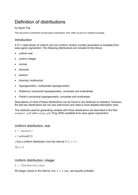
<strong>Definition</strong> <strong>of</strong> <strong>distributions</strong><br />
by <strong>Agner</strong> <strong>Fog</strong><br />
This document is published at www.agner.org/random, Feb. 2008, as part <strong>of</strong> a s<strong>of</strong>tware package.<br />
Introduction<br />
A C++ class library <strong>of</strong> uniform and non-uniform random number generators is available from<br />
www.agner.org/random. The following <strong>distributions</strong> are included in this library:<br />
• uniform real<br />
• uniform integer<br />
• normal<br />
• bernoulli<br />
• poisson<br />
• binomial, multinomial<br />
• hypergeometric, multivariate hypergeometric<br />
• Wallenius' noncentral hypergeometric, univariate and multivariate<br />
• Fisher's noncentral hypergeometric, univariate and multivariate<br />
Descriptions <strong>of</strong> most <strong>of</strong> these <strong>distributions</strong> can be found in any textbook on statistics. However,<br />
the last two <strong>distributions</strong> are not very well known and need a more detailed description here.<br />
The methods used for generating variates with these <strong>distributions</strong> are described in the files<br />
sampmet.pdf and nchyp.pdf (<strong>Fog</strong> 2004) available from www.agner.org/random.<br />
Uniform distribution, real<br />
x = Random()<br />
x ~ uniform(0,1)<br />
x has a uniform distribution over the interval 0 ≤ x < 1.<br />
f( x ) =<br />
1<br />
Uniform distribution, integer<br />
x = IRandom(min,max)<br />
All integer values in the interval min ≤ x ≤ max are equally probable.
1<br />
f( x ) =<br />
max−<br />
min+<br />
1<br />
Normal distribution<br />
x = Normal(m,s)<br />
x ~ normal(m,s)<br />
Normal distribution with mean m and standard deviation s. This distribution simulates the sum <strong>of</strong><br />
many random contributions.<br />
1<br />
f( x)<br />
= ‰<br />
2πs<br />
( x−<br />
m)<br />
−<br />
2s<br />
2<br />
Bernoulli distribution<br />
x = Bernouilli(p)<br />
x ~ binomial(1,p)<br />
2<br />
Describes a situation with two possible outcomes. The probability <strong>of</strong> success is p.<br />
f( 0)<br />
= 1 − p , f( 1)<br />
= p<br />
Poisson distribution<br />
x = Poisson(L)<br />
x ~ poisson(λ)<br />
This is the distribution <strong>of</strong> the number <strong>of</strong> events in a given time span or a given geographical<br />
area when these events are randomly scattered in time or space.<br />
x λ −λ<br />
f( x)<br />
= ‰<br />
x!<br />
Binomial distribution<br />
x = Binomial(n,p)<br />
x ~ binomial(n,p)<br />
This is the distribution <strong>of</strong> the number <strong>of</strong> red balls you get when drawing n balls with replacement<br />
from an urn where p is the fraction <strong>of</strong> red balls in the urn.
⎛n<br />
⎞<br />
f( x)<br />
= ⎜ ⎟ p ( 1 )<br />
⎝ x⎠<br />
x n−<br />
x − p<br />
Multinomial (multivariate binomial) distribution<br />
Multinomial(x,p,n,c)<br />
x ~ mbinomial(p,n,c)<br />
This distribution extends the urn experiment with replacement to any number <strong>of</strong> colors, c. pi is<br />
the fraction <strong>of</strong> balls <strong>of</strong> color i in the urn. n is the number <strong>of</strong> balls you take. xi is the number <strong>of</strong><br />
balls <strong>of</strong> color i you get in the sample.<br />
f(x )<br />
=<br />
n!<br />
c<br />
∏<br />
∏ =<br />
c<br />
i 1 xi!<br />
i = 1<br />
p<br />
xi<br />
i<br />
Hypergeometric distribution<br />
x = Hypergeometric(n,m,N)<br />
x ~ hyp(n,m,N)<br />
This is the distribution <strong>of</strong> the number <strong>of</strong> red balls you get when drawing n balls without<br />
replacement from an urn where m is the number <strong>of</strong> red balls in the urn and N is the total number<br />
<strong>of</strong> balls in the urn.<br />
f( x)<br />
=<br />
⎛<br />
⎜<br />
⎝<br />
m<br />
x<br />
⎞⎛<br />
⎟⎜<br />
⎠⎝<br />
⎛<br />
⎜<br />
⎝<br />
N −<br />
n −<br />
N ⎞<br />
⎟<br />
n ⎠<br />
m⎞<br />
⎟<br />
x ⎠<br />
Multivariate hypergeometric distribution<br />
MultiHypergeo(x,m,n,c)<br />
x ~ mhyp(m,n,c)<br />
This distribution extends the urn experiment without replacement to any number <strong>of</strong> colors, c. mi<br />
is the number <strong>of</strong> balls <strong>of</strong> color i in the urn. N is the total number <strong>of</strong> balls in the urn. n is the<br />
number <strong>of</strong> balls you take. xi is the number <strong>of</strong> balls <strong>of</strong> color i you get in the sample.<br />
f(x<br />
)<br />
=<br />
c ⎛mi<br />
⎞<br />
⎜<br />
⎟<br />
1 ⎝ x ⎠<br />
⎛ N ⎞<br />
⎜ ⎟<br />
⎝ n ⎠<br />
∏<br />
i = i
Wallenius' Noncentral hypergeometric distribution, univariate and<br />
multivariate<br />
x = WalleniusNCHyp(n,m,N,w)<br />
MultiWalleniusNCHyp(x,m,w,n,c)<br />
x ~ mwnchyp(n,m,ω)<br />
This distribution models an urn experiment without replacement, with bias. Assume that an urn<br />
contains N balls <strong>of</strong> c different colors. mi is the number <strong>of</strong> balls <strong>of</strong> color i. The balls have different<br />
weight (or size) which makes the sampling biased. The probability that a particular ball <strong>of</strong> color i<br />
is taken is proportional to its weight wi. The univariate distribution is the special case c = 2.<br />
Note that there are two 'noncentral hypergeometric' <strong>distributions</strong> which are <strong>of</strong>ten confused in the<br />
literature. These two <strong>distributions</strong> are distinguished here by the prefix names Wallenius' and<br />
Fisher's.<br />
The univariate Wallenius' noncentral hypergeometric distribution is defined by Wallenius (1963)<br />
and the multivariate distribution by Chesson (1976):<br />
⎛ c ⎛m<br />
⎞⎞<br />
1<br />
c<br />
c<br />
i ⎜∏<br />
⎟<br />
ω<br />
⎜ ⎜<br />
⎟<br />
i / d xi<br />
f( x ) =<br />
⎟∫<br />
∏ ( 1 − t ) „ t , where d = ∑ ω i ( m<br />
0<br />
⎝ i = 1 ⎝ xi<br />
⎠⎠<br />
i = 1<br />
i = 1<br />
∑ xi = n , ∑ mi = N<br />
i<br />
− x )<br />
Description <strong>of</strong> various properties <strong>of</strong> this distribution, calculation methods and sampling methods<br />
are given in <strong>Fog</strong> (2008a,b).<br />
Fisher's noncentral hypergeometric distribution, univariate and multivariate<br />
x = FishersNCHyp(n,m,N,w)<br />
MultiFishersNCHyp(x,m,w,n,c)<br />
x ~ mfnchyp(n,m,w)<br />
This distribution resembles Wallenius' noncentral hypergeometric distribution, and unfortunately<br />
it is <strong>of</strong>ten given the name 'noncentral hypergeometric distribution' (e.g. McCullagh & Nelder<br />
1989). A less common name for this distribution is the extended hypergeometric distribution<br />
(Harkness 1965, Johnson & Kotz 1969).<br />
Fisher's noncentral hypergeometric distribution is defined as a conditional distribution. Let xi be c<br />
independent binomial variates with the <strong>distributions</strong><br />
xi ~ binomial(mi, pi), i = 1.. c<br />
then the distribution <strong>of</strong> x on the condition that ∑ xi = n is the (multivariate) Fisher's noncentral<br />
hypergeometric distribution.<br />
This distribution is not normally associated with the metaphor or taking colored balls from an<br />
urn, but here I will apply an urn model, however farfetched, for the sake <strong>of</strong> analogy with<br />
Wallenius' noncentral hypergeometric distribution. You are taking n balls without replacement<br />
from an urn containing balls <strong>of</strong> c different colors. The balls have different weights wi which make<br />
i
the sampling biased in favor <strong>of</strong> the heavier balls. Before taking the balls you assign to each ball<br />
a probability pi <strong>of</strong> being taken. These probabilities are preferably calculated so that the expected<br />
total number <strong>of</strong> balls taken is n. Now you take or don't take each ball according to the assigned<br />
probabilities and count the total number <strong>of</strong> balls taken. If this number is not equal to n then put<br />
all the balls back in the urn and repeat the experiment. You may have to repeat this experiment<br />
many times before you have a sample containing exactly n balls.<br />
The relationship between pi and wi is given by<br />
p<br />
i<br />
rwi<br />
=<br />
1 + rw<br />
i<br />
where the scale factor r is adjusted so that ∑ mi pi<br />
= n .<br />
The distribution function is<br />
f( x)<br />
=<br />
=<br />
f1(<br />
x)<br />
, where<br />
f ( y)<br />
∑<br />
y∈S<br />
1<br />
⎛m<br />
⎞<br />
⎟<br />
⎝ ⎠<br />
c<br />
∏ ⎜<br />
i = 1 xi<br />
x<br />
i<br />
i i<br />
f ( x ) w , and the support<br />
1<br />
S<br />
⎧<br />
⎨x<br />
∈ Ù<br />
⎩<br />
c<br />
c = 0 + | ∑ xi<br />
= n<br />
i=<br />
1<br />
⎫<br />
⎬<br />
⎭<br />
Description <strong>of</strong> various properties <strong>of</strong> this distribution, calculation methods and sampling methods<br />
are given in <strong>Fog</strong> (2008b).<br />
References<br />
Chesson, J (1976): A non-central multivariate hypergeometric distribution arising from biased<br />
sampling with application to selective predation. Journal <strong>of</strong> Applied Probability, vol. 13, no. 4,<br />
pp. 795-797.<br />
<strong>Fog</strong>, <strong>Agner</strong> (2008a): Calculation Methods for Wallenius' Noncentral Hypergeometric Distribution.<br />
Communications in Statistics - Simulation and Computation. vol. 37, no. 2, pp. 258-273.<br />
<strong>Fog</strong>, <strong>Agner</strong> (2008b): Sampling Methods for Wallenius' and Fisher's Noncentral Hypergeometric<br />
Distributions. Communications in Statistics - Simulation and Computation. vol. 37, no. 2, pp.<br />
241-257.<br />
Harkness, W L (1965): Properties <strong>of</strong> the Extended Hypergeometric Distribution. Annals <strong>of</strong><br />
Mathematical Statistics, vol. 36, no. 3, pp. 938-945.<br />
Johnson, N L & Kotz, S (1969): Distributions in Statistics, 1: Discrete Distributions. Boston:<br />
Houghton Mifflin Co.<br />
McCullagh, P & Nelder, J A (1989): Generalized Linear Models. 2. ed. London: Chapman &<br />
Hall.<br />
Wallenius, K T (1963): Biased Sampling: The Non-central Hypergeometric Probability<br />
Distribution. Ph.D. thesis, Stanford University.


