Measurement and Evaluation of Subgrade Soil Parameters

MEASUREMENT AND EVALUATION OF
SUBGRADE SOIL PARAMETERS:
pHASE I - SYNTHESIS OF lITERATURE
FHWA/MT-09-006/8199
prepared for
THE STATE OF MONTANA
DEPARTMENT OF TRANSPORTATION
Final Report
in cooperation with
THE U.S. DEPARTMENT OF TRANSPORTATION
FEDERAL HIGHWAY ADMINISTRATION
September 2009
prepared by
Dr. Robert Mokwa, P.E.
Michelle Akin
College of Engineering
Western Transportation Institute
Montana State University - Bozeman
R E S E A R C H P R O G R A M S

You are free to copy, distribute, display, and perform the work; make derivative works; make
commercial use of the work under the condition that you give the original author and sponsor
credit. For any reuse or distribution, you must make clear to others the license terms of this
work. Any of these conditions can be waived if you get permission from the sponsor. Your fair
use and other rights are in no way affected by the above.

Measurement and Evaluation of
Subgrade Soil Parameters:
Phase I – Synthesis of Literature
Final Project Report
Prepared by:
Dr. Robert Mokwa, P.E.
Associate Professor, Civil Engineering Department
and
Michelle Akin
Research Associate, Western Transportation Institute
of the
College of Engineering/Western Transportation Institute
Montana State University - Bozeman
Prepared for:
State of Montana
Department of Transportation
Research Programs
in cooperation with the
U.S. Department of Transportation
Federal Highway Administration
September 2009

TECHNICAL REPORT DOCUMENTATION PAGE
1. Report No.:
FHWA/MT-09-006/8199
2. Government Access No.: 3. Recipient’s Catalog No.:
4. Title and Subtitle:
5. Report Date: September 2009
Measurement and Evaluation of Subgrade Soil Parameters:
Phase I – Synthesis of Literature
6. Performing Organization Code:
7. Author(s): Robert Mokwa and Michelle Akin 8. Performing Organization Report Code:
9. Performing Organization Name and Address:
10. Work Unit No.:
Montana State University/Western Transportation Institute
Civil Engineering Dept., Bozeman, Montana 59717
11. Contract or Project No.:8199
12. Sponsoring Agency Name and Address:
13. Type of Report and Period Covered:
Research Programs
Final Report
Montana Department of Transportation
November 2008 – September 2009
2701 Prospect Avenue
Helena, Montana 59620-1001
15. Supplementary Notes:
14. Sponsoring Agency Code: 5401
Research performed in cooperation with the Montana Department of Transportation and the U.S.
Department of Transportation, Federal Highway Administration. This report can be found at
http://www.mdt.mt.gov/research/docs/research_proj/subgrade_soils/final_report.pdf
16. Abstract:
A key material property used in the mechanistic-empirical pavement design guide (MEPDG) is the
resilient modulus (Mr), which either can be obtained from experimental testing or can be
backcalculated from other measured soil properties. The determination of a representative Mr value for
a given subgrade, considering seasonal variations and testing intricacies, is not an easy or
straightforward task. Over 30 different correlations equations were reviewed in this study. Selected
equations were further examined using data from two MDT soil survey reports. Results from the
literature review and preliminary data evaluation indicate there is little to no consistency between
equations for predicting Mr from soil index and classification properties. Most of the equations were
developed from relatively small sample sets and often for region-specific soil types.
Until a more detailed assessment is conducted, the authors discourage the general use of Mr correlation
equations without prior testing and verification of the suitability and reliability of the modulus
estimates. The authors suggest that full scale implementation of a repeated load triaxial testing
program for the determination of Mr on a routine project basis may not be the most cost effective
approach for MDT. Rather, it is recommended that additional evaluation of MDT soil survey data be
conducted to identify potentially useful correlation equations and to identify the soil parameters that
may be most denotative of soil stiffness. A subsequent phase of focused repeated load triaxial testing
could then be conducted in an efficient manner to measure Mr for specific soil types and to verify the
suitability and applicability of previously identified correlation equations.
17. Key Words:
Resilient modulus, mechanistic-empirical pavement design
guide, R-value, CBR, Mr correlations, repeated load triaxial
tests
19. Security Classif. (of this
report): Unclassified
20. Security Classif. (of this
page): Unclassified
18. Distribution Statement:
No restrictions. This document is
available through National Tech. Info.
Service, Springfield, VA 22161.
21. No. of Pages: 66 22. Price:
Montana State University/Western Transportation Institute ii

DISCLAIMER STATEMENT
This document is disseminated under the sponsorship of the Montana Department of
Transportation and the United States Department of Transportation in the interest of information
exchange. The State of Montana and the United States Government assume no liability of its
contents or use thereof.
The contents of this report reflect the views of the authors, who are responsible for the facts
and accuracy of the data presented herein. The contents do not necessarily reflect the official
policies of the Montana Department of Transportation or the United States Department of
Transportation.
The State of Montana and the United States Government do not endorse products of
manufacturers. Trademarks or manufacturers' names appear herein only because they are
considered essential to the object of this document.
This report does not constitute a standard, specification, or regulation.
ALTERNATIVE FORMAT STATEMENT
MDT attempts to provide accommodations for any known disability that may interfere with
a person participating in any service, program, or activity of the Department. Alternative
accessible formats of this information will be provided upon request. For further information,
call (406) 444-7693, TTY (800) 335-7592, or Montana Relay at 711.
ACKNOWLEDGEMENTS
Acknowledgement of financial support for this research is extended to the Montana
Department of Transportation and the Montana State University Civil Engineering Department.
Montana State University/Western Transportation Institute iii

EXECUTIVE SUMMARY
Executive Summary
A critical component of highway pavement design involves a thorough and reliable
characterization of the subgrade; i.e., the foundation of the pavement riding surface. Laboratory
test methods are available to characterize the strength and stiffness of subgrade soils including
the Resistance value (R-value), California Bearing Ratio (CBR), and repeated load triaxial tests.
In-situ tests that have been used to evaluate subgrade properties include, among others: falling
weight deflectometer, in-situ CBR, plate load, miniature cone penetrometer, and dynamic cone
penetrometer tests.
A key material property used in the mechanistic-empirical pavement design guide (MEPDG)
is the resilient modulus (Mr), which either can be obtained from laboratory testing or can be
backcalculated from other measured soil properties. The determination of a representative Mr
value for a given subgrade, considering seasonal variations and testing intricacies, is not an easy
or straightforward task. The standard laboratory repeated-load triaxial compression test
(AASHTO T307) is complex, time-consuming, and costly, and is likely not warranted for all soil
types.
Because of uncertainties in testing methods and the large diversity of subgrade soils across
the U.S., numerous correlation equations for estimating Mr are available in the technical
literature and new equations continue to appear on a rather frequent basis. These correlations
were typically developed for specific groups of soil types or for soils obtained from specific
geographic regions. Most Mr correlation equations were developed using regression analyses in
which RLT resilient modulus test results were compared to results obtained from less expensive
or more routine tests, such as R-value, CBR, unconfined compression, and index property tests.
Over 30 different correlation equations were reviewed in this study. Selected equations were
further examined using data from two MDT soil survey reports. The evaluation indicated there
is little to no consistency between equations for predicting Mr from soil index and classification
properties. Most of the equations were developed from relatively small sample sets and often for
region-specific soil types. Until a more detailed assessment is conducted, the authors discourage
general use of any correlation equation without prior testing and verification of the suitability
and reliability of the equation for use in specific applications.
An extensive number of correlation equations have been developed over the past 20 years.
We believe it would be prudent to conduct additional analyses of existing data to help narrow the
field of equations and focus subsequent testing programs on specific soil types and soil
parameters. We suggest that full scale implementation of a repeated load triaxial testing program
for the determination of Mr on a routine project basis may not be the most cost effective
approach for MDT. Rather, it is recommended that additional evaluation of MDT soil survey
data be conducted to identify potentially useful correlation equations and to identify soil
parameters that may be most denotative of soil stiffness. A subsequent phase of focused RLT
testing could then be conducted in an efficient manner to measure Mr for specific soil types and
to verify the suitability and applicability of previously identified correlation equations.
Montana State University/Western Transportation Institute iv

TABLE OF CONTENTS
Contents
1 INTRODUCTION ........................................................................................................................1
2 TEST METHODS FOR SUBGRADE EVALUATION ..............................................................3
2.1 Laboratory Tests for Subgrade Evaluation ................................................................................3
2.2 Field Tests for Subgrade Evaluation ..........................................................................................6
2.3 Summary ....................................................................................................................................9
3 CORRELATION EQUATIONS FOR RESILIENT MODULUS ..............................................10
3.1 R-value Correlation Equations .................................................................................................10
3.2 CBR Correlation Equations .....................................................................................................13
3.3 Soil Property Correlation Equations ........................................................................................16
3.4 Summary ..................................................................................................................................24
4 EVALUATION OF CORRELATIONS AND THE RLT TEST ................................................29
4.1 Introduction ..............................................................................................................................29
4.2 R-value Correlation Equations .................................................................................................29
4.3 CBR Correlation Equations .....................................................................................................31
4.4 Soil Property Correlation Equations ........................................................................................32
4.5 Evaluation of MDT Repeated Load Triaxial Mr Data .............................................................37
4.6 Sensitivity Analysis .................................................................................................................39
4.7 Repeated Load Triaxial Test Equipment .................................................................................41
4.8 Summary ..................................................................................................................................43
5 CONCLUSIONS AND RECOMMENDATIONS .....................................................................45
5.1 Summary and Conclusions ......................................................................................................45
5.2 Recommendations ....................................................................................................................45
REFERENCES ..................................................................................................................................47
APPENDIX A – COMPARISON OF RLT TEST PROTOCOLS ...................................................52
Montana State University/Western Transportation Institute v

LIST OF TABLES
Contents
Table 2.1. Typical Confining and Deviatoric Stress Values, from Hossain 2008 ......................... 6
Table 3.1. Evaluation of the Asphalt Institute R-value Correlation Equations (adapted from
Asphalt Institute 1982) .......................................................................................................... 11
Table 3.2. Summary of Correlation Equations for Resilient Modulus ........................................ 26
Table 4.1. Assumptions Utilized in the Correlation Equations ................................................... 34
Table 4.2. Comparison of Correlation Ratios: Mr-correlation/Mr-AASHTO 1993 .................................... 36
Table 4.3. Statistical Summary of Data from Von Quintus and Moulthrop (2007) Tests ........... 38
Table 4.4. Baseline Conditions for Sensitivity Study ................................................................... 40
LIST OF FIGURES
Figure 1. Relationship between CBR, Group Index and AASHTO classification (adapted from
ODOT 2008). ........................................................................................................................ 15
Figure 2. Example plot illustrating the breakpoint modulus concept. ......................................... 17
Figure 3. Typical values of Mr for AASHTO classified soils (data from NCHRP 1-37A, 2004).
............................................................................................................................................... 23
Figure 4. Typical values of Mr for USCS classified soils (data from NCHRP 1-37A, 2004). .... 24
Figure 5. Scanned plot from MDT Surface Design Manual. ....................................................... 30
Figure 6. Resilient modulus based on R-value correlations. ....................................................... 31
Figure 7. Resilient modulus based on CBR correlations. ............................................................ 32
Figure 8. Mr correlation using MDT soil survey data. ................................................................. 36
Figure 9. Normal distribution of Mr correlation equations. ......................................................... 37
Figure 10. Correlated Mr values compared to RLT measured Mr. .............................................. 38
Figure 11. Normal distribution of Mr from correlation equations. .............................................. 39
Figure 12. Sensitivity of flexible pavement Structural Number to Mr as a function of daily
ESALs. .................................................................................................................................. 41
Figure 13. Cross-section of typical triaxial setup (from AASHTO T307). ................................. 43
Montana State University/Western Transportation Institute vi

1 INTRODUCTION
Introduction
Although a pavement’s wearing course is most prominent, the success or failure of a
roadway section is often dependent upon the underlying subgrade. The strength, stiffness,
compressibility and moisture characteristics of the subgrade can have significant influences on
pavement performance and long-term maintenance requirements. The subgrade must be strong
enough to resist shear failure and have adequate stiffness to minimize vertical deflection.
Stronger and stiffer materials provide a more effective foundation for the riding surface and will
be more resistant to stresses from repeated loadings and environmental conditions.
A critical component of the pavement design involves a thorough and reliable
characterization of the subgrade; i.e., the foundation of the pavement riding surface. A number
of laboratory methods are available to characterize the strength and stiffness of subgrade soils
including the Resistance value (R-value), California Bearing Ratio (CBR), and repeated load
triaxial laboratory tests. In-situ tests that have been used to evaluate subgrade properties include,
among others: falling weight deflectometer (FWD), in-situ CBR, plate load, miniature cone
penetrometer, and dynamic cone penetrometer tests. Several state transportation agencies are
evaluating the potential of using correlations with index tests such as Atterberg limits and grain
size distributions for estimating soil parameters for use in mechanistic pavement design methods.
Many soils in Montana pose significant problems for constructability and long-term
pavement performance. The current method (R-value testing) used by the Montana Department
of Transportation (MDT) to quantify the suitability of these soils for subgrade strength may yield
unsatisfactory or inconsistent results. Other investigatory techniques may yield more consistent
and reliable results, which will improve pavement performance and save significant construction
and maintenance funds.
A key material property used in the AASHTO pavement design guide and the new
mechanistic-empirical pavement design method is the resilient modulus (Mr), which is defined as
the ratio of deviatoric stress to elastic (resilient) strain experienced by the material under
repeated cycles of loading. The determination of a representative Mr value for a given subgrade,
considering seasonal variations and testing intricacies, is not an easy or straightforward task.
The standard laboratory repeated-load triaxial compression test (AASHTO T307) is complex,
time-consuming, and costly, and is likely not warranted for all soil types.
Because of uncertainties in testing methods and the large diversity of subgrade soils across
the U.S., numerous empirical and semi-empirical correlations for estimating Mr are available in
the technical literature. These correlations were typically developed for specific groups of soil
types or for soils obtained from specific geographic regions. There is no currently recognized or
unified general approach for using correlation equations, and the reliability of these equations is
often uncertain. Most correlations are site or region specific, and most correlations do not
account for important variations in soil type and consistency. Adding to the confusion are the
various modifications, adjustments, and simplifications that have been proposed as
improvements to the laboratory repeated load triaxial test method for determining Mr. For
example, the proceedings from the 2008 meeting of the Transportation Research Board in
Washington D.C. contained seven papers on alternative methods for measuring, correlating, or
Montana State University/Western Transportation Institute 1

Introduction
estimating Mr. Even with the recent escalation of work in this area, some agencies still rely on
rather dated and quite general correlation charts such as those first published in the 1960s by the
Portland Cement Association and the Federal Highway Administration (Terrel et al. 1979).
This report provides a synthesis and overview of laboratory and in-situ test methods that
have been used by state agencies and researchers to measure the stiffness of unbound base
courses and subgrade soils. The focus of the literature synthesis is on methods for measuring Mr;
either indirectly using correlations with other more readily measured soil parameters, or directly
using laboratory and in-situ test methods. Data from two MDT soil survey reports were used to
conduct a preliminary comparison of selected correlation equations. Results from the synthesis
and analyses are summarized in Chapter 5 and specific recommendations are provided for
implementation by MDT.
Montana State University/Western Transportation Institute 2

Test Methods for Subgrade Evaluation
2 TEST METHODS FOR SUBGRADE EVALUATION
In recent decades, characterization of the subgrade for purposes of pavement design has
focused on the engineering behavior (stress-strain response) of the soil caused by traffic loads.
Resilient modulus is the primary soil parameter for most pavement design methodologies in the
U.S. While the repeated load triaxial (RLT) test is widely recommended as a test method for
determining resilient modulus, other laboratory and field methods have been used to estimate
resilient modulus, including California Bearing Ratio (CBR), Resistance Value (R-value), and
Falling Weight Deflectometer (FWD), among others. This chapter provides information about
laboratory and field test methods that can be used to characterize the subgrade for pavement
design.
2.1 Laboratory Tests for Subgrade Evaluation
Tests can be conducted in the laboratory on remolded soil samples or relatively undisturbed
field specimens. Some methods are conducted at specific moisture-density conditions such as:
optimum, near optimum, worst-case, or at various moisture-density permutations to illustrate
potential variations in stiffness as the soil water content changes throughout the year. A few test
methods reportedly provide a “better” resilient modulus value because of more advanced test
protocols and control of stress, strain, and pore pressures; whereas, other tests are merely related
to resilient modulus based on empirical correlations. The correlation approach is often chosen
because of past experience and lack of evidence that more complicated and expensive tests are
necessary. This section provides an overview of laboratory and in-situ tests used for subgrade
characterization and for estimating a resilient modulus for pavement design.
2.1.1 R-value
The resistance value (R-value) of a soil is determined with remolded soil samples in a
stabilometer device after finding the exudation pressure. Soil specimens are prepared in a
kneading compactor at different near-saturation water contents and placed in an exudation
indicator device and tested in compression at a rate of 2000 pounds per minute. After the
exudation pressure is recorded, loading is stopped to allow the soil to rebound. The soil is then
placed in a stabilometer and a horizontal pressure of 5 psi induced. A displacement-controlled
vertical load is applied at 0.05 inches per minute until the load reaches 2000 pounds. The
horizontal pressure is recorded before the vertical load is reduced to 1000 pounds and the
horizontal pressure reduced to 5 psi. Finally, the number of turns on a calibrated handle (referred
to as turns displacement) required to increase the horizontal pressure from 5 to 100 psi is
determined. The R-value is calculated based on the turns displacement and the horizontal
pressure corresponding to the 2000-pound vertical load. The calculated R-value can range
between 0 and 100, although values less than 5 are usually reported as “minus 5,” “-5,” or “

Test Methods for Subgrade Evaluation
aggregate source. Additional details of the test apparatus and protocol are provided in ASTM
D2844 and AASHTO T190.
R-value is not intrinsically related to resilient modulus; nevertheless, it is still used as a test
method by several state DOTs because of its familiarity and historical use in pavement design.
Numerous correlations have been developed to relate the R-value of a soil to resilient modulus; a
selection of these correlations are presented in Chapter 3.
The R-value test is performed on soil samples prepared at different water contents to
generate a range of exudation pressures between 100 and 800 psi. The R-value corresponding to
a specific exudation pressure can be interpolated. For pavement design, MDT uses the R-value
corresponding to 300 psi exudation pressure.
2.1.2 California Bearing Ratio
The California bearing ratio (CBR) is determined with remolded soil samples in a load
frame in which a two-inch-diameter piston is forced 0.5 inches into the soil surface at a constant
rate of 0.05 inches per minute. The load associated with 0.1-inch and 0.2-inch displacements of
the soil is compared to a “standard” load of 1,000 and 1,500 psi for a crushed aggregate material.
Cylindrical 6-inch diameter, 4.58-inch tall soil samples are prepared in a 7-inch tall mold. The
additional height provides space for surcharge weights, which represent the overburden pressure
caused by the overlying pavement section. Usually, several soil samples are prepared at different
water contents that are typically referenced to the optimum Proctor water content. After
compaction, the samples are typically soaked for 96 hours, unless instantaneous “end of
construction” CBR values are desired. The mold base and a surface plate are slotted to allow
water to enter the soil specimen from both ends. The surcharge weights are in place for the
soaking period and during the penetration step. Additional details of the test apparatus and
protocol are provided in ASTM D1883 and AASHTO T193. Plastic clayey subgrades tend to
have CBR values less than about 5; whereas, base course aggregates tend to have CBR values
greater than about 40.
Like R-value, CBR is not inherently related to resilient modulus. In any case, the test is still
used by several state DOTs in lieu of the more expensive and time consuming repeated load
triaxial resilient modulus test. Correlations to facilitate pavement design have been developed to
relate CBR to resilient modulus; these correlations are discussed in Chapter 3.
2.1.3 Repeated Load Triaxial Resilient Modulus Test
The repeated load triaxial (RLT) test can be conducted on remolded or undisturbed field
samples. The test is conducted on samples in a triaxial chamber and performed at various levels
of confining pressure (σ3) and various levels of repeated deviatoric stress (σd). The deviatoric
stress (σd) is the difference between the total axial stress (σ1) and the confining pressure (σ3).
The test was designed to better simulate the loads induced by traffic than the R-value and CBR
tests.
Considerable research and development has been conducted to further refine details of the
test method. The AASHTO standards for this test have been revised and replaced several times
since the first standard was adopted in 1982. Sometimes revisions to a protocol were deemed too
Montana State University/Western Transportation Institute 4

Test Methods for Subgrade Evaluation
dissimilar to merely revise the existing standard; in this case a new standard (with a new number)
was adopted. Because of this, the following historic AASHTO standards for resilient modulus of
unbound materials have existed; in chronological order they are: T274, T292, T294, and TP46.
The current AASHTO standard for RLT determination of resilient modulus is T307, which
replaced the four previous standards that were subsequently withdrawn. AASHTO T307 is
based largely on the Strategic Highway Research Program’s (SHRP) Long Term Pavement
Performance Program’s (LTPP) efforts to modify previous AASHTO standards to provide more
consistent and repeatable test results. Subsequent to the adoption of T307, additional standards
have been proposed, including NCHRP Project 1-28 in 1997 and Project 1-28A in 2004, which
provided a protocol that reportedly harmonized the 1-28 protocol with the AASHTO standards.
The NCHRP 1-28A proposed standard is written in AASHTO format, but as of this writing it has
not formally been adopted as an AASHTO standard. Appendix A provides a table with details of
each test protocol and emphasizes the wide variation in how RLT resilient modulus tests have
been conducted. Unfortunately, there is not an acceptable method to cross-relate resilient
modulus parameters obtained from different test protocols (Puppala 2008).
Puppala (2008) provides a comprehensive synthesis of literature pertaining to laboratory
resilient modulus tests, including RLT test method development and effects of compaction, soil
type, confining pressure, deviatoric stress, instrumentation, and data analysis. The following
points are noted from Puppala’s (2008) NCHRP synthesis:
Research prior to 1986 primarily addressed development of RLT test protocols
and apparatus, models for data analysis, and correlations to soil strength and index
properties.
Research between 1986 and 1996 primarily addressed repeatability and reliability
issues of RLT tests; methods for quantifying the effects of soil type, preparation
and compaction procedures; and models used for data analysis. This period also
witnessed a growing database of resilient modulus test results for soils in various
localized regions, although not all used the same RLT test protocol.
Research after 1996 has been dominated by state DOT-sponsored projects in
which laboratory RLT resilient modulus tests were performed on region-specific
materials. These studies included topics such as: recommendations to modify or
simplify the test protocols, comparisons between laboratory RLT tests and various
field tests, and evaluation of analytical methods for calculating the resilient
modulus for pavement design.
RLT testing is the preferred laboratory method to determine resilient modulus for
subgrade characterization needed for pavement design.
State DOTs are hesitant to adopt routine RLT resilient modulus testing because of
continual modifications to standardized test procedures.
In lieu of conducting laboratory RLT tests, use of local correlations is considered
preferable to correlations developed for national use.
Montana State University/Western Transportation Institute 5

Test Methods for Subgrade Evaluation
As part of a RLT resilient modulus testing program on Arkansas subgrade soils, Elliott et al.
(1988) used elastic layer theory to estimate the deviator stress (σd or σcyclic) induced by a 9000 lb
wheel load for typical pavement cross sections. Results from the study indicate that variations in
σd can be estimated based on the structural number of the pavement system. The deviator stress
is approximately equal to 4 psi for structural numbers greater than 2.5 and approximately 8 psi
for structural numbers less than 2.
Using an elastic layer analysis method, George (2004) calculated typical stress states for
Mississippi subgrade soils under a 4500 lb wheel load to be σd = 7.4 psi and lateral confining
stress (σ3 or σc) = 2 psi.
Mohammad et al. (2007) reported that on average typical subgrade stress levels from the
literature were σd = 6 psi and σ3 = 2 psi.
Hossain (2008) tabulated a collection of σd and σ3 values that were used in various research
projects cited in the literature. Based on a synthesis of the values shown in Table 2.1, Hossain
chose to use σd = 6 psi and σ3 = 2 psi.
Table 2.1. Typical Confining and Deviatoric Stress Values, from Hossain 2008
Confining Stress
(psi)
(σc or σ3)
Deviatoric Stress
(psi)
(σd or σcyclic)
Reference
2 5.4 Rahim (2005)
2 7.4 George (2004)
2 5 Ping et al. (2001)
2 6 Asphalt Institute (as cited by Ping et al. 2001)
2 2 Daleiden et al. (as cited by Ping et al. 2001)
3 6 Lee et al. (1997)
2 6 Jones and Witczak (1977)
Part 2, Chapter 1, Section 2.1.3.4 of the MEPDG design guide (NCHRP 1-37A, 2004)
provides a procedural outline for calculating σd and σ3 using elasticity theory, the coefficient of
lateral earth pressure at rest (ko) and the densities of overlying soil and pavement layers.
2.2 Field Tests for Subgrade Evaluation
Field tests can provide measurements of resilient modulus and other soil parameters for the
conditions existing at the site at the time the test is conducted. Thus, consideration should be
given to the influence of climate and in-situ conditions on the measured parameters relative to
design needs. Tests conducted in the field to characterize subgrade soils for pavement design
can be categorized in two broad categories: 1) nondestructive or 2) intrusive. Nondestructive
methods usually involve the measurement of small deformations induced by an impulse load;
Montana State University/Western Transportation Institute 6

Test Methods for Subgrade Evaluation
whereas, intrusive methods are often based on penetration of standard pistons or cones (Puppala
2008). This section provides information about field tests used for subgrade characterization and
how in-situ tests can be used to determine resilient modulus.
2.2.1 Falling Weight Deflectometer (FWD) and Lightweight FWD
Falling weight deflectometers can be used to determine the moduli of pavement layers by
inducing an impulse load on the surface and measuring deflections with geophones. The moduli
are determined from the measurements using iterative back-calculation computer programs.
Numerous computer programs are available; unfortunately, these programs can yield inconsistent
results and different moduli values. According to Puppala (2008), the two most commonly used
back-calculation programs are EVERCALC and MODULUS. According to Alavi et al. (2008),
DARWin and ELMOD are the most commonly used programs. In general, a modulus
determined by FWD will be higher than a modulus determined from RLT resilient modulus tests.
Thus, AASHTO recommends a correction of 0.33 to 0.5 be applied to moduli determined by
FWD. The study by Ping et al. (2002) confirmed AASHTO’s correction factors, while other
studies suggest a smaller correction may be more appropriate (e.g., Rahim and George 2003).
The FWD test is used by at least 45 state DOTs. Ninety percent of these states use the FWD to
estimate pavement layer moduli according to a recent survey conducted by Alavi et al. (2008) for
NCHRP Synthesis 381. Puppala (2008) provides a comprehensive overview of research
sponsored by state DOTs involving the use of FWDs and Lightweight or Portable FWDs.
2.2.2 Dynamic Cone Penetration Test
The dynamic cone penetrometer (DCP) device consists of a cylindrical rod with a cone tip
that is driven into the soil by repeatedly dropping a 17.6 or 10.1 pound weight from a height of
22.6 inches. The cone tip has a 60° angle and a 0.8-inch-diameter base. Disposable tips can be
used in which the tip remains in the soil when the rod is extracted. The cumulative penetration is
measured and recorded with the number of blows. Penetration readings are typically measured
for each blow in soft soils and every 5 or 10 blows in stiffer soils. For rehabilitation or
reconstruction design, only small cores (diameter as little as one inch) need to be drilled through
the pavement surface to expose the underlying unbound materials for DCP investigation. After
several decades of research, ASTM D6951 was adopted in 2003 to standardize the apparatus and
protocol for shallow pavement applications. The ASTM standard provides a correlation between
DCP index and in-situ CBR based on research conducted by the U.S. Army Corps of Engineers.
Several other correlations have been proposed to determine elastic and resilient modulus from
DCP index, which can be found in Puppala (2008).
2.2.3 Plate Load Test
A plate load test is conducted by applying an axial load to a set of steel bearing plates and
observing the deflection of the soil. A set of up to four one-inch-thick plates with diameters
ranging from 6 to 30 inches are stacked in a pyramid fashion. The bottom plate is seated firmly
on the soil layer using fine sand and/or plaster of Paris as a leveling aid. Dial gauges are used to
measure vertical deflection as the plates are loaded with a hydraulic jack connected to heavy
mobile equipment or to a structure, which provide a reaction against the loading.
Montana State University/Western Transportation Institute 7

Test Methods for Subgrade Evaluation
ASTM D1195 describes the process for loading the plates in a repetitive manner in which a
load is applied and maintained until the rate of deflection is less than 0.001 inches per minute,
for three minutes. The load is then released, the soil rebound measured, and the same load
reapplied six times. Load and deflection are continually monitored during the load and unload
cycles. The loading cycles are repeated at two consecutively higher axial loads.
ASTM D1196 and AASHTO T222 describe the process for non-repetitive loading, in which
load is applied in increments until a predetermined total deflection is obtained or the load
capacity of the equipment is reached. Each load increment is held constant until the rate of
deflection is less than 0.001 inches per minute for three minutes before the next load increment is
applied. The standards do not provide specific methods for interpreting the bearing capacity of
the soil; however, instructions are provided to create plots that could be used in analysis or
design.
2.2.4 In-Situ CBR
The in-situ CBR test procedure is analogous to the laboratory procedure in which the load
required to penetrate a two-inch diameter piston into soil at a rate of 0.05 inches per minute is
measured. Loading is usually obtained by a manually operated jack with reaction provided by a
stiff beam connected to heavy mobile equipment. The field procedure uses 10-inch diameter
surcharge weights; whereas, smaller six-inch outer diameter weights are used in the laboratory
test because additional confinement is provided by the mold. Specific details of the test
apparatus and procedure are provided in ASTM D4429.
2.2.5 Dilatometer Test
A dilatometer (DMT) test provides an estimate of the lateral in-situ modulus. A drill rig or
other field equipment outfitted with a hydraulic press is used to push a flat steel blade into the
soil. At selected depths, a thin circular steel membrane located on one side of the blade is
expanded with pressurized gas. Gravels and aggregates can damage the sensitive membrane;
consequently, the DMT is primarily used to test sands and fine-grained soils. Details of the test
procedure are provided in ASTM D6635. Borden et al. (1985) reported the DMT test correlated
well with unsoaked CBR values for A-5 and A-6 soils. Borden et al. (1986) later published a
relationship between dilatometer modulus and constrained modulus. Additional testing and
research is necessary to establish a reliable relationship between these moduli and the resilient
modulus.
2.2.6 Cone Penetration Test
Cone penetration testing (CPT) is increasingly common with geotechnical sections of state
DOTs according to a recent survey reported in NCHRP Synthesis 368 (Mayne 2007). During a
cone penetration test, an instrumented cone is pushed into the soil and measurements of cone tip
resistance, sleeve friction, and sometimes pore pressure are electronically recorded. The CPT
provides useful geotechnical and geoenvironmental information on soils and groundwater at
depth. However, the device is not commonly used to obtain properties at very shallow depths
(less than about 2 ft) because of the relatively low confining pressures near the ground surface in
relationship to the size of the cone. Mohammad et al. (2007) developed resilient modulus
Montana State University/Western Transportation Institute 8

Test Methods for Subgrade Evaluation
correlations using a nonstandard standard miniature CPT probe (Continuous Intrusion Miniature
CPT) for fine and coarse-grained Louisiana subgrade soils. Based on our literature review, it
appears these correlations are not used widely outside the state of Louisiana.
2.3 Summary
This chapter provides information regarding laboratory and field tests that can be used for
subgrade characterization for purposes of pavement design. Recent pavement design methods
such as the 1986 and 1993 AASHTO design guides and the new mechanistic-empirical pavement
design procedure characterize the subgrade in terms of resilient modulus. The RLT laboratory
test method was designed to determine the resilient modulus of a soil sample, but the test
protocol has changed several times since it was first introduced in the 1980s. A detailed
comparison of eight versions of the test protocol is provided in Appendix A. All of these
methods have been used at one time or another for both research and design purposes.
Consequently, databases and research publications that contain RLT test results may not always
be comparable, especially for establishing correlations with other soil properties.
Other laboratory test methods that were used for subgrade characterization prior to the use
of resilient modulus are the CBR and R-value tests. These tests are still conducted by several
state DOTs for pavement design by utilizing a correlation between CBR or R-value and resilient
modulus. The Falling Weight Deflectometer is the most widely used field test for subgrade
characterization of existing roads. A number of other in-situ methods have been used with
limited success at estimating Mr, including: dynamic cone penetration, miniature cone
penetration, plate load, in-situ CBR, dilatometer tests.
Montana State University/Western Transportation Institute 9

Correlation Equations for Resilient Modulus
3 CORRELATION EQUATIONS FOR RESILIENT MODULUS
The resilient modulus approach was first incorporated into pavement analysis and design in
the 1980s after several decades of research. Since that time, there has been significant effort to
relate the resilient modulus to more readily measured soil parameters using index and strength
tests. One noteworthy complication to such an evaluation is the lack of a widely accepted test
procedure to measure resilient modulus. Many laboratory and field approaches have been
proposed; consequently, it is important to examine the specific details of any study before
applying a correlation equation in design or before incorporating a correlation equation into an
agency-wide standard. Specific details that could significantly affect the reliability of any
correlation equation include resilient modulus test protocols as well as information on the soil
type and moisture conditions. This chapter summarizes previous research attempts to establish
correlations between Mr and more readily measured soil parameters. Whenever possible, testing
details and soil conditions are documented with the applicable equations.
3.1 R-value Correlation Equations
3.1.1 Buu (1980)
The Idaho Transportation Department (ITD) commissioned a study in the late 1970s to
develop a correlation between resilient modulus and R-value (Buu 1980). The RLT test was
used to measure Mr and then correlated to the R-value test result. The RLT tests were conducted
at the University of Idaho using customized triaxial equipment and the R-value tests were
conducted at ITD headquarters in Boise, Idaho. The correlation equations are reported in Yeh &
Su (1989) as:
M r ( ksi)
= 1. 455
+ 0.
057×
R
(1)
M r ( ksi)
= 1. 600
+ 0.
038×
R
(2)
The correlations correspond to resilient modulus test conditions of σd = 6 psi and σ3 = 2 psi.
Where σd is the vertical deviatoric stress and σ3 is the lateral confining pressure. Eq. (1) was
developed from tests on 10 fine-grained soils with R-values between 46 and 68; Eq. (2) was
developed from tests on 14 coarse-grained soils with R-values between 9 and 82 (Yeh and Su
1989, Sandefur 2003).
The coefficient of determination (R 2 value) of a regression equation indicates the ability of
the equation to predict the outcome of a given set of inputs. An R 2 value close to unity indicates
the data fits the correlation equation very well. The R 2 values for Eq.s (1) and (2) are 0.10 and
0.82, respectively (Yeh and Su 1989), indicating Eq. (2) is a better predictor of Mr for the soil
samples considered in the analysis.
Tri Buu was contacted by the authors of this study to learn more information about the
history of the equations because various attempts to locate the research report were unsuccessful.
The phone conversation revealed that recent advances in data acquisition and displacement
sensors cast doubt on the validity of the results that were generated in the study. ITD no longer
Montana State University/Western Transportation Institute 10

Correlation Equations for Resilient Modulus
uses these correlation equations. It is our understanding that ITD recently purchased a resilient
modulus testing machine to develop a new database of test results to correlate Mr and R-value
(Tri Buu, personal communication, February 26, 2009).
3.1.2 Asphalt Institute (1982)
The Asphalt Institute (1981) design method recommends that RLT tests be performed to
characterize the subgrade soil for pavement design. However, because many state DOTs do no
have the necessary equipment to perform laboratory resilient modulus tests, the Asphalt Institute
(1982) also provides two correlation equations. Eq. (3) was developed based on data collected
from road tests in San Diego County (California) during the 1960s and 70s.
Mr ( ksi)
= 0.
772 + 0.
369×
R
(3)
Additional evaluations by the Asphalt Institute (1982) led to Eq. (4), which was
implemented in the thickness design manual (Asphalt Institute 1981), although no details were
provided about whether additional soils were tested.
( ksi)
= 1. 155 + 0.
555×
R
M r (4)
To evaluate the applicability of these equations, the Asphalt Institute extended the original
study to include R-value and Mr tests on six additional soils. The results are summarized in
Table 3.1. For these six soils, the sum of the squared errors (SSE), between the predicted and
actual Mr, indicate Eq. (3) is actually a better predictor overall than Eq. (4) (SSE = 258 and 863,
respectively). When considering soils with lower R-values (R < 21), Eq. (4) is more applicable
based on the sum of the squared errors (SSE = 94 for Eq. (3) and SSE = 38 for Eq. (4)).
However, Asphalt Institute (1982) cautions that when applied to higher R-value soils (i.e., R >
60), the correlations tend to overestimate Mr beyond a level appropriate for pavement design.
Table 3.1. Evaluation of the Asphalt Institute R-value Correlation Equations (adapted
from Asphalt Institute 1982)
Soil Type R-value a Mr (ksi) b
Mr (Eq. 3) Mr (Eq. 4)
Prediction Error
(ksi)
c
Prediction Error
(%) (ksi)
c
(%)
Sand 60 16.9 22.9 36 34.5 104
Silt 59 11.2 22.5 101 33.9 203
Sandy loam 21 11.6 8.5 -27 12.8 10
Silt-clay loam 21 17.6 8.5 -52 12.8 -27
Silty-clay 18 8.2 7.4 -9.6 11.0 34
Heavy clay

Correlation Equations for Resilient Modulus
Based on the small quantity of test data and the large range of percent error, it is
recommended that only limited confidence be placed in these correlation equations.
3.1.3 Washington Department of Transportation
The Washington Department of Transportation (WSDOT) developed a relationship between
R-value and resilient modulus by testing soils ranging from coarse aggregates (A-1) to silty and
clayey materials (A-7). R-values were measured according to WSDOT’s test method in which
the R-value is determined at an exudation pressure of 400 psi. The soils in this study had Rvalues
between 25 and 75. RLT resilient modulus tests were conducted according to AASHTO
T274. The reported correlation between R-value and Mr had an R 2 value of 0.67 (Muench et al.
2009).
M
r
0.
0521×R
( ksi)
= 0.
72(
−1.
0)
e (5)
3.1.4 Colorado Department Transportation
Colorado Department of Transportation (CDOT) developed a multi-stepped correlation that
converts soil support value to an R-value then R-value to an approximation of Mr (Yeh and Su
1989). Soil support value was used in the 1961 and 1972 AASHTO pavement design guides to
characterize the subgrade soil until it was replaced with resilient modulus in the 1986 design
guide. The soil support value varied between 1 and 10 and was determined indirectly by CDOTs
past experience or from R-value or CBR test results (Yoder and Witczak 1975, Huang 1993,
George 2004). Eq. (6) shows the correlation from R-value to Mr, but no information was
presented to document the soils or Mr test protocols used to develop the equation.
a
M r ( ksi)
= 0.
001×
10
(6)
where a = { ( R − 5 ) / 11.
29 + 21.
72}
6.
24
[ ]
3.1.5 Yeh and Su (1989)
Yeh and Su (1989) developed a correlation for CDOT based on lab tests conducted on 19
soil samples. The initial phase of testing was conducted in 1985 on six clays with R-values
between 5 and 40. We developed the following linear equation by applying a regression analysis
to the Yeh and Su (1989) data.
Mr ( ksi)
= 1. 859
+ 0.
219×
R
(7)
The R 2 value for this equation is 0.97, which indicates a relatively good fit with the data used to
develop the equation.
In a subsequent phase of testing, 13 additional soils were tested, including a wider variety of
Colorado cohesionless subgrade soils. The resilient modulus was determined at the Advanced
Soils Lab at the University of Colorado at Denver and the R-value was determined at CDOT.
The RLT tests used to measure resilient modulus were reportedly performed in substantial
Montana State University/Western Transportation Institute 12

Correlation Equations for Resilient Modulus
accordance to AASHTO T274. The 19 soils were compacted to 95% of standard Proctor density
(AASHTO T99); 16 were saturated prior to Mr testing and three were tested at optimum water
content. The six clay soils were tested at σ3 = 0, 3, and 6 psi and σd = 2, 5, 7, and 10 psi. The
other 13 soils were tested at σ3 = 3 and 6 psi and σd = 1, 2, 4, and 8 psi. The R-value test was
conducted according to CDOT’s procedure, which is similar to the AASHTO procedure. The
reported R-value corresponded to an exudation pressure of 300 psi. After the Mr test, 10 soils
were re-tested using the R-value method to quantify any change in R-value. For this unusual retest
conducted on 10 of the samples, the R-value increased for two soils, decreased for seven
soils (average decrease of 24), and remained unchanged for 1. The silty soils were most
susceptible to a decrease in R-value when re-tested, which may be indicative of the sensitivity
and the difficulty in obtaining repeatable results for these types of soils. The average of the pre-
and post-Mr R-values were computed for these 10 soils. No correction was applied to the other
nine soils in the development of the correlation; instead, the R-values prior to the Mr tests were
used. In other words, no distinction was made between soils that were re-tested and those that
were tested only once.
The results of this subsequent testing yielded the following equation by Yeh and Su (1989)
for a confining pressure of 3 psi and a deviatoric stress of 6 psi.
( ksi)
= 3. 5 + 0.
125×
R
M r (8)
We plotted the reported data and calculated an R 2 value of approximately 0.5. The average
(absolute) percent difference between the actual and calculated Mr for all samples is 22 percent.
There is more variation for R-values greater than 60, suggesting additional soils in this range
should be tested to further calibrate the method.
3.1.6 1993 AASHTO design
The correlation equation in the 1993 AASHTO pavement design guide is similar to Eq. (2)
from the Asphalt Institute except the intercept is slightly different (as reported by Puppala 2008).
The following equation is reportedly valid for fine-grained soils with R-values less than or equal
to 20.
M r ( ksi)
= 1. 0 + 0.
555×
R
(9)
3.2 CBR Correlation Equations
3.2.1 Heukelom & Klomp (1962)
Heukelom and Klomp (1962) developed a commonly referenced CBR correlation based on
dynamic modulus measurements and in-situ CBR tests. The in-situ CBR test results were
correlated with moduli measurements obtained using an instrumented vibratory compactor in the
field; not from RLT tests in a laboratory. A correlation was developed based on a combination
of three sets of data:
1) wave velocity data reported by Jones (1958) for CBR values between 2 and 20,
Montana State University/Western Transportation Institute 13

Correlation Equations for Resilient Modulus
2) wave velocity measurements conducted by Heukelom and Klomp (1962) for CBR
values between 3 and 200, and
3) stiffness measurements conducted by Heukelom and Klomp (1962) for CBR values
between 3 and 200.
Heukelom and Klomp (1962) used these three data sets to calculate a dynamic modulus
from the wave velocity. Even though Heukelom and Klomp (1962) did not refer to the modulus
as a resilient modulus, the study is presented herein because their correlation equation (Eq. 10) is
referenced in several sources; sometimes as Heukelom and Klomp (1962) and sometimes as the
Shell Laboratory method (Asphalt Institute 1982, Drumm et al. 1990, Witczak et al. 1995,
Sukumaran et al. 2002, Puppala 2008).
M r
( ksi)
1.
42 × CBR
= (10)
While the regression coefficient of 1.42 provides the best fit for 69 test results with CBR values
ranging from 2 to 200, it could easily vary from 0.7 to 2.8 because of the large scatter in the data.
Most references to Eq. (10) in the literature simply round the coefficient to 1.5, which is likely a
result of this wide range. Lofti (1984) postulated that the lack of a term for deviatoric stress in
the model is responsible for the wide scatter in the data. Most references indicate the correlation
is only reasonable for soils with CBR values less than 10 or less than 20. Again, there are some
inconsistencies in how the original Heukelom and Klomp (1962) work is presented in later
publications.
3.2.2 Green & Hall (1975)
The US Army Corps of Engineers developed the Mr and CBR relationship shown in Eq. (11)
by comparing vibratory wave propagation measurements to in-situ CBR measurements obtained
at several different road test projects (Green and Hall 1975). Similar to Heukelom and Klomp
(1962), the correlation provides dynamic modulus, not resilient modulus. Data with CBR values
from 2 to 200 were included in the database used to develop Eq. (11).
0.711
M ( ksi)
= 5.
409 × CBR
(11)
r
3.2.3 Powell et al. (1984)
In the course of developing a structural design method for asphalt roads in the United
Kingdom, Powell et al. (1984) created a correlation equation for subgrade characterization based
on in-situ CBR tests and wave propagation techniques. The study’s authors did not use
laboratory RLT tests because at the time of their research the authors reportedly believed that
RLT tests were still primarily a research tool and not yet suitable for routine applications.
Powell et al. (1984) incorporated a database of measurements originally published by Jones
(1958), which involved 23 data points with CBR values all less than 20. Eq. (12) developed by
Powell et al. (1984) includes empirical modifications to account for strain discontinuity between
in-situ CBR tests (high strain), wave propagation tests (low strain), and vehicle-induced strains.
Montana State University/Western Transportation Institute 14

0.64
( ksi)
2.
554 CBR
Correlation Equations for Resilient Modulus
M = ×
(12)
Unfortunately, no information about soil types or the theoretical or empirical corrections used to
determine Eq. (12) was published. Powell et al. (1984) indicated the equation is only applicable
for soils with CBR values between 2 and 12.
3.2.4 Lofti (1984) and Lofti et al. (1988)
Lofti (1984) and Lofti et al. (1988) developed a relationship between resilient modulus and
CBR in which the deviatoric stress is included as a model parameter. Laboratory CBR and RLT
resilient modulus tests were performed on a fabricated pulverized kaolinite clay (USCS
classification = ML, with LL = 48 and PI = 42) at 13 different moisture-density permutations.
The unsoaked CBR values ranged from 2 to 21. The RLT tests were conducted at σ3 = 3 psi with
σd = 3, 5, 10, 15, 20, 40, and 80 psi. Lofti (1984) used their measured data along with additional
data from Barker (1982) to develop Eq. (13), which had an R 2 = 0.93 for the test data. The units
of σd are psi in Eq. (13).
⎛ logσ d ⎞
log M r ( ksi)
= 1.0016 + 0.043(
CBR)
-1.9557⎜
⎟ − 0.1705 logσ d (13)
⎝ CBR ⎠
3.2.5 Ohio DOT (2008)
The Ohio Department of Transportation (ODOT) uses a correlation that relates Mr to CBR;
however, instead of measuring CBR directly, CBR is estimated based on the group index (GI) of
the soil, which is a function of the liquid limit (LL), plasticity index (PI), and percent passing the
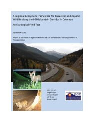
No. 200 sieve (p#200). After GI is calculated, the CBR is estimated from Figure 1, and Eq. (14)
is used to calculate Mr.
Figure 1. Relationship between CBR, Group Index and AASHTO classification
(adapted from ODOT 2008).
M r
( ksi)
1.
2 × CBR
= (14)
Montana State University/Western Transportation Institute 15

Correlation Equations for Resilient Modulus
3.2.6 South African Council
The South African Council on Scientific and Industrial Research (CSIR) uses Eq. (15) to
estimate Mr from laboratory CBR results (reported by Witczak et al. 1995 and Sukumaran et al.
2002):
0.65
M ( ksi)
= 3.
0×
CBR
(15)
r
No additional information about the resilient modulus test method or the soil types used to
develop the equation is available. The original source of the equation was not provided in the
cross-references and the authors of the current study were not able to locate the original
published work despite extensive attempts.
3.3 Soil Property Correlation Equations
3.3.1 Jones & Witczak (1977)
Jones & Witczak (1977) developed two correlation equations for A-7-6 subgrade soils in
California. Resilient modulus RLT tests were performed at σd = 6, 12, and 18 psi and σ3 = 2, 4,
6, 8, and 12 psi. The regression equations can be used to calculate Mr at specific stresses (σd = 6
psi and σ3 = 2 psi) by inputting water content (w) and degree of saturation (S):
1) Eq. (16) is based on Mr results of 10 remolded soil samples compacted to modified
Proctor density (R 2 = 0.94):
( ksi)
= −0.
1328 + 0.
0134S
2.
319
log M r w +
(16)
2) Eq. (17) is based on Mr results of 97 undisturbed field samples (R 2 = 0.45):
( ksi)
= −0.
1111 + 0.
0217S
1.
179
log M r w +
(17)
where, w is the water content and S is the degree of saturation. Jones and Witczak (1977)
postulated that one possible reason for the differences between Eq.s (16) and (17) is that the
remolded samples compacted wet of optimum may have had a dispersed structure; whereas, the
undisturbed field samples most likely had a natural flocculated structure.
3.3.2 Robnett and Thompson (1973) and Thompson and Robnett (1979)
Thompson and Robnett (1979) tested A-4, A-6, and A-7 Illinois subgrade soils from 50
locations around the state. The soils were compacted with a kneading-type action to 95 or 100
percent of standard Proctor density at optimum, optimum plus 1%, or optimum plus 2% water
contents. The samples were cured for seven days before undergoing RLT resilient modulus
testing. All resilient modulus tests were performed at zero confining pressure. The axial stress
path was approximately triangular-shaped and a load duration of 60 milliseconds was used.
After applying 1,000 axial load applications for the conditioning step, a deviatoric stress of 3 psi
was applied for 10 repetitions and then slowly increased at 3 to 5 psi increments for 10
repetitions until substantial permanent deformation was observed (this usually occurred at a
deviatoric stress of about 25 psi). The stress applied for the conditioning step varied between 7
Montana State University/Western Transportation Institute 16

Resilient Modulus (M r )
6
5
4
3
2
1
σd ≅ 6 psi
Deviator Stress (σ d )
Correlation Equations for Resilient Modulus
and 22 psi, depending on the soaked CBR value of the subgrade. The conditioning stress was
determined for each soil based on the anticipated vertical load of an Illinois Class III flexible
pavement with a 9,000 pound dual wheel load at 80 psi tire pressure (Robnett and Thompson
1973).
A plot of resilient modulus versus deviator stress exhibited a bilinear trend in which the
resilient modulus decreased as deviator stress increased. The resilient modulus associated with
the intersection of the two lines is termed the breakpoint resilient modulus, as shown in Figure 2.
The slope was steeper for deviator stresses less than 6 psi and then shallower (about 85 percent
less steep) for increasing values of deviator stress above 6 psi (Thompson and Robnett 1979).
breakpoint M r
0
0 5 10 15 20 25
Figure 2. Example plot illustrating the breakpoint modulus concept.
Multiple linear regression analyses of the breakpoint resilient modulus (the resilient modulus
corresponding to a deviator stress of approximately 6 psi for the soils tested) indicated the
modulus was primarily a function of several different soil parameters. Eq. (18) yielded the
strongest relationship (R 2 = 0.64) between Mr and soil index properties, in which Mr is a function
of plasticity index (PI), percent silt (%SILT), percent clay (%CLAY), percent organic carbon
(%OC), and group index (GI):
(a)
M r
( ksi)
= 6.37 + 0.450(
PI)
− 0.0038(
%SILT)
+ 0.034(
%CLAY)
−1.64(
%OC)
− 0.244(
GI)
Rather than Eq. (18), Illinois DOT uses Eq. (19), which has a lower R 2 value (0.40), but requires
fewer parameters than Eq. (18), (Marshall Thompson, personal communication, April 16, 2009).
Montana State University/Western Transportation Institute 17
(18)

Correlation Equations for Resilient Modulus
Additionally, when Thompson and LaGrow (1988) developed a flexible pavement design
procedure for Illinois DOT, they chose Eq. (19) to provide the relationship for a representative
subgrade resilient modulus value.
(b) ( ksi)
4.46 + 0.098(
%CLAY)
+ 0.119(
PI)
M r
= (19)
Thompson and Robnett (1979) developed Eq. (20) by correlating the breakpoint resilient
modulus to measured unconfined compressive strength (qu in psi). Eq. (20) had an R 2 value of
0.47 using the measured test data.
q 0.307 0.86 ksi = +
(20)
(c) ( ) u
M r
Thompson and Robnett (1979) also examined the effects of degree of saturation (S) on
resilient modulus and developed the following two correlations. Eq. (21) gives the breakpoint
resilient modulus (Mr at σd = 6 psi) for soils compacted to 95% standard Proctor dry density,
whereas Eq. (22) is for 100% standard Proctor dry density. The R 2 values are 0.41 and 0.50,
respectively.
(d) ( ksi)
= 32.
9 − 0.
334×
S
(e) ( ksi)
= 45.2
− 0.428×
S
where, S is the degree of saturation.
Mr (21)
Mr (22)
3.3.3 Carmichael and Stuart (1985)
Carmichael and Stuart (1985) collected over 3,300 resilient modulus records from tests
conducted on 250 soils from across the U.S. to develop a correlation for the U.S. Forest Service.
As a result of missing data points and other complications in the regression analyses, two
formulations were developed:
1) Eq. (23) for fine-grained soils (CH, MH, ML, and CL) was based on 418 data points
(R 2 = 0.76):
M
r
( ksi)
= 37.43−
0.457(
PI)
− 0.618w
− 0.142(
p#200)
+ 0.179σ − 0.325σ + 36.42(
CH)
+ 17.10(
MH)
3
w = water content (%)
p#200 = % passing the #200 sieve
PI = plasticity index
CH = 1 for CH soil, 0 otherwise
MH = 1 for MH soil, 0 otherwise
Montana State University/Western Transportation Institute 18
d
(23)

Correlation Equations for Resilient Modulus
2) Eq. (24) for coarse-grained soils (GW, GP, GM, GC, SW, SP, SM, and SC) was
based on 583 data points (R 2 = 0.84):
( ksi)
= 0.
523−
0.0225 + 0.544 logσ
+ 0.
173(
SM)
+ 0.197(
GR)
Mr T
w
w = water content (%)
σT = total stress (σd + 3σ3)
SM = 1 for SM soil, 0 otherwise
GR = 1 for GM, GW, GC, or GP soils, 0 otherwise
(24)
3.3.4 Elliott et al. (1988)
Elliott et al. (1988) investigated the effect of compaction, moisture, freeze-thaw, and
combinations of confining and deviator stresses on the resilient modulus of 15 Arkansas
subgrade soils. Most of the soils were classified as A-4, A-6, and A-7 with the exception of a
single A-2 soil. All resilient modulus tests were performed following the AASHTO T274 RLT
test procedure using three confining pressures (σ3 = 0, 3, and 6 psi) and five deviator stresses (σd
= 1, 2, 4, 8, and 10 psi). In addition to the RLT tests conducted to correlate resilient modulus to
soil properties, the authors employed a simplification to the RLT test procedure using fewer load
cycles and fewer deviator stresses.
Two correlation equations were developed based on the “backward elimination” regression
technique. Resilient modulus was most sensitive to percent clay (%CLAY), plasticity index (PI),
and optimum water content (wopt), although other factors were considered (maximum dry
density, liquid limit, percent colloids, and percent organic content). Eq. (25) was recommended
for computing a resilient modulus corresponding to σd = 4 psi (R 2 = 0.80). Eq. (26) was
recommended for computing a resilient modulus corresponding to σd = 8 psi (R 2 = 0.77).
r
( ksi)
11.21+
0.17(
%CLAY)
+ 0.20(
PI)
− 0.73 opt
( ksi)
9.
81+
0.13(
%CLAY)
+ 0.16(
PI)
− 0.60 opt
Mr = w
(25)
M = w
(26)
3.3.5 Drumm et al. (1990)
Drumm et al. (1990) developed correlation equations based on the breakpoint resilient
modulus, using an approach similar to the one used by Thompson and Robnett (1979). The
resilient modulus test was performed according to the AASHTO T274 RLT test procedure on 11
sources of A-2, A-4, A-6, and A-7 Tennessee subgrade soils at zero confining pressure.
Unconfined compressive strength tests were conducted on samples in the triaxial cell
immediately after completing each Mr test. Index tests were also performed.
Unconfined compressive strength test data were analyzed to determine the modulus at the
initial portion of the stress-strain curve (at a stress well below the yield stress) because the lower
strain range was deemed more compatible with the small measured strains of resilient modulus
tests. In general, the initial portion of the modulus (E) versus strain (ε) curve was approximately
Montana State University/Western Transportation Institute 19

Correlation Equations for Resilient Modulus
linear. The inverse of the y-intercept of this plot was termed the initial tangent modulus (1/a,
with units of psi).
Eq. (27) was developed using a backward elimination regression technique. The properties
that most significantly correlated to breakpoint resilient modulus at σd = 6 psi were initial tangent
modulus (1/a), unconfined compressive strength (qu, in psi), plasticity index (PI), dry unit weight
(γd, in pcf), degree of saturation (S), and percent passing No. 200 sieve (p#200). The R 2 value
was 0.83 for 22 tests (11 soils each at two different water contents).
M
r
⎡
⎢
⎣
⎛ 1 ⎞
⎜ ⎟
⎝ a ⎠
+ 0.45
PI − 0.216γ − 0.25S
( ksi)
0.001 45.8 + 0.00052 + 0.188q +
= u
( ) 0.15(
p#200)]
d −
Drumm et al. (1990) developed a second more general equation for a range of deviator
stresses using the same resilient modulus test results. In addition to the parameters used in the
previous equation, Eq. (28) also requires percent clay (%CLAY) and liquid limit (LL).
M
r
( ksi)
a'+
b'σ
d
=
σ
d
a'=
318.2
+ 2.26
+ 0.
337q
u + 0.
73(
% CLAY)
( PI)
− 0.915γ − 2.
19S
− 0.304(
p#200)
⎛ 1 ⎞
b'=
2.10 + 0.
00039⎜
⎟ +
⎝ a ⎠
0.
104q
+ 0.
09
( LL)
− 0.10(
p#200)
Eq. (28) was developed with data for σd ranging from 2.5 to 25 psi. For the correlation of a', R 2
= 0.81 and for the correlation of b', R 2 = 0.73. The overall R 2 value for the equation based on the
Mr results of each value of σd tested was 0.80, suggesting a relatively good fit to the test data.
However, the expression appears to be less accurate at lower values of σd because of the
hyperbolic nature of the equation.
3.3.6 Farrar and Turner (1991)
Farrar and Turner (1991) collected nine clayey and four silty subgrade soils from Wyoming
and developed two resilient modulus correlation equations, which were based on: 1) R-value test
results and 2) soil index properties. Clayey soils (A-6 and A-7-6) and silty soils (A-4) were
included in the research. Resilient modulus was determined with RLT test equipment
conforming to AASHTO T274 and performed at σ3 = 0, 3, and 6 psi and σd = 4, 8, and 10 psi.
Specimens were compacted using a kneading-type compactor to three different target densities:
1) standard Proctor density at minus 1% of optimum water content, 2) standard Proctor density at
plus 2% of optimum water content, and 3) the moisture and density corresponding to the
conditions of the R-value specimens at 300 psi exudation pressure. The 4 inch diameter, 8-inch
long specimens were compacted in four layers.
Montana State University/Western Transportation Institute 20
u
(27)
(28)

Correlation Equations for Resilient Modulus
The clayey soils all had reported R-value results of minus five; consequently, the authors
decided a different approach was necessary to develop a reliable correlation. A modified Rvalue
procedure was developed for 4-inch diameter 2.5-inch tall samples. Specimens were
compacted using two layers instead of four. The R-value was determined with a Hveem
stabilometer according to AASHTO T190 except the exudation and swell phases of the test were
not performed. The clayey soils produced modified R-values between 10 and 50. The silty soils
produced modified R-values between 9 and 64.
The correlation equation (Eq. 29) between modified R-value (Rm) and natural logarithm of
resilient modulus requires the user to input whether the soil is clayey or silty according to the
AASHTO classification system. The R 2 value for the data used to develop Eq. (29) was 0.59.
a
( ksi)
0.
001
Mr = e
(29)
a = 7.
16 + 0.
0389R
− 0.
049σ
+ 0.
040σ
+ 1.
01X
m
d
Xc = 1 for clayey soils, 0 otherwise
A separate correlation was developed based on degree of saturation (S), plasticity index (PI),
and percent passing the No. 200 sieve (p#200). The R 2 value for the data used to develop Eq.
(30) was 0.66.
( ksi)
M r = 30.
280 − 0.
359S
− 0.
325σ
d + 0.
237σ
c
+ 0.086
( PI)
+ 0.
107(
p#200)
3.3.7 Rahim and George (2004)
Rahim and George (2004) conducted 180 RLT resilient modulus tests on Mississippi
subgrade soils in accordance with AASHTO TP46. Undisturbed Shelby tube samples were
collected for laboratory RLT tests at depths ranging from 1 to 3 ft below the subgrade from 60
locations on two Mississippi roads (SR25 and US45). The subgrade soil on SR25 classified as
A-6; whereas, US45 had A-2-4, A-3, and A-6 subgrade soils. Correlation equations (31) and
(32) were developed for fine-grained and coarse-grained soils, respectively, at σd = 5.4 psi and σ3
= 2 psi.
1) Fine grained soils, 77 samples (R 2 = 0.70):
M
r
( ksi)
⎡⎛
LL γ
= 2.
429⎢
⎜ ×
⎢⎣
⎝ w γ d
d
−s
p#200 ⎞
⎟
100 ⎠
Montana State University/Western Transportation Institute 21
⎞
⎟
⎠
2.
06
⎛
+ ⎜
⎝
2) Coarse-grained soils, 49 samples (R 2 = 0.75):
M
r
( ksi)
⎛ γ d ⎞
= 44.
58⎜
⎟
⎝ w ⎠
0.
86
⎛ p#200 ⎞
×
⎜
log ⎟
⎝ Cu
⎠
−0.
46
−0.
59
3
⎤
⎥
⎥⎦
c
(30)
(31)
(32)

Correlation Equations for Resilient Modulus
where, LL is the liquid limit, w is the water content, p#200 is the percent passing the #200 sieve,
γd-s is the maximum standard Proctor dry density, γd is the in-situ dry density, and Cu is the
uniformity coefficient.
Of the 180 resilient modulus tests performed, 70 percent of the test results (representing 126
samples) were used to develop the two correlation equations. The other 30 percent of the data
was used to check the models by comparing the laboratory results to the predicted Mr values
using the correlation equations. Measured and predicted Mr values for the 33 additional finegrained
samples compared well, with an R 2 value of 0.75 for Eq. (31). The measured and
predicted Mr values for the 21 additional coarse-grained samples showed even better agreement,
with an R 2 value of 0.82 for Eq. (32).
In a separate study, George (2004) compared the results of AASHTO TP46 RLT resilient
modulus test results from eight Mississippi test sections to values predicted by seven correlation
equations, including the two developed by Rahim and George (2004). Two test sections had
coarse-grained subgrade soils and the other six had fine-grained subgrade soils; none of the test
sections were used in the development of Eq.s (30) and (31). The best agreement between
measured and predicted values was obtained when Eq. (30) was used. This supports the premise
that correlations developed for localized regions (such as a single state) likely provide better
estimates of resilient modulus than equations developed for nationwide or nonspecific soil
conditions. Consistent use of the same RLT test protocol for both the George (2004) and the
Rahim and George (2004) testing may have also contributed to the relatively good agreement
between predicted and measured results.
3.3.8 Resilient Modulus in MEPDG Computation Models
Pavement response computation models incorporated into the mechanistic-empirical design
approach require the input of Mr values to represent the stiffness of supporting layers, which
include unbound granular base materials and subgrade soils. The MEPDG identifies a 3-level
hierarchical approach for inputting resilient moduli based on the significance of the project.
For Input Level 1, the designer conducts specific tests to measure Mr directly. The
recommended standard laboratory methods for modulus testing are NCHRP 1-28A and
AASHTO T307. The general resilient modulus constitutive equation recommended in the
mechanistic-empirical design procedure is as follows:
k
2
3
⎛ θ ⎞ ⎛τ
oct ⎞
M r = k1
pa
⎜
1
p ⎟
⎜ +
a p ⎟
(33)
⎝ ⎠ ⎝ a ⎠
where, Mr is the resilient modulus in psi, θ is the bulk stress, τoct is the octahedral shear stress
(τoct = σ1 + σ2 + σ3), σ1, σ2, σ3 are principal stresses, and pa is the atmospheric pressure.
Dai and Zollars (2002) refer to this as the “universal model” because the equation is
applicable for all unbound materials and it incorporates the effects of both deviatoric and
volumetric stresses on Mr. For rehabilitation and reconstruction of existing pavement layers, Mr
values for input Level 1 can also be obtained by performing nondestructive testing using a falling
weight deflectometer. Input Level 1 provides the most accurate results with the highest
Montana State University/Western Transportation Institute 22
k

Correlation Equations for Resilient Modulus
reliability and lowest level of uncertainty. However, this level of input requires extensive effort
and is the highest cost option of the three input categories.
For Input Level 2, general correlation equations that include soil index and strength
properties are used to estimate Mr. These relationships can be direct or indirect such as the
numerous correlation equations described in this chapter that are based on R-value, CBR, soil
classification, etc. The correlation equations are empirically based and have been developed on
local levels as well as regional and national approximations. Level 2 input provides an
intermediate echelon of accuracy for pavement design and is the most commonly used approach
by state transportation agencies (Puppala 2008).
For Input Level 3, Mr is estimated from experience or historical records. For example, the
mechanistic-empirical design guide provides a table of typical representative Mr values covering
a wide range of soil types. Approximate Mr values in the MEPDG range from about 40,000 psi
for A-1-a granular soils to about 8,000 psi for A-7-6 clayey soils. Figure 3 shows a distribution
of Mr for soil types based on the AASHTO soil classification system and Figure 4 shows a
typical Mr distribution for soil types based on the Unified Soil Classification System (USCS).
The data in these plots was obtained from Table 2.2.51, Chapter 2 of the MEPDG (NCHRP 1-
37A, 2004). Level 3 inputs, such as the typical values presented in Figure 3 and Figure 4,
provide the lowest level of accuracy. Level 3 input values should only be used for designs in
which there are “minimal consequences of early failure” (NCHRP 1-37A, 2004). The plots of
typical Mr values may also be useful as a check on laboratory or field measured values of Mr
(e.g., Level 1 input) or as a check on the reasonableness of soil property correlations (e.g., Level
2 input).
Resilient Modulus, M r (psi)
45000
40000
35000
30000
25000
20000
15000
10000
5000
0
A-1-a A-1-b A-2-4 A-2-5 A-2-6 A-2-7 A-3 A-4 A-5 A-6 A-7-5 A-7-6
AASHTO Soil Classification
approximate M r range
Figure 3. Typical values of Mr for AASHTO classified soils (data from NCHRP 1-37A,
2004).
Montana State University/Western Transportation Institute 23

Resilient Modulus, M r (psi)
45000
40000
35000
30000
25000
20000
15000
10000
5000
0
USCS Soil Classification
Correlation Equations for Resilient Modulus
approximate M r range
GW GP GM GC SW SP SM SC ML CL MH CH
Figure 4. Typical values of Mr for USCS classified soils (data from NCHRP 1-37A, 2004).
3.3.9 Other types of correlations
In general, the correlation equations described in this chapter were developed using
regression analyses in which RLT resilient modulus test results were compared to the results of
less expensive or more routine tests, such as R-value, CBR, unconfined compression, and index
tests. These are classified as direct correlations by Puppala (2008). Indirect correlation
equations take the form of Mr = f(σd, σ3, other σ expressions, k1, k2, k3,…ki) in which the k1, k2,
k3, …ki parameters are correlated to soil properties. The indirect correlations are created by
conducting a series of RLT resilient modulus tests on various soils and analyzing the results of
each test with any of the two, three, or four parameter models mentioned in Chapter 2. The k1,
k2, k3, … ki parameters are then determined for each test and are referred to as “measured”
parameters. By correlating the measured parameters to soil properties (such as LL, PI, %CLAY,
w, S, etc), the resilient modulus of other similar soils can be estimated at a variety of stress states
without conducting another RLT test. Puppala (2008) provides a review of various indirect
correlation attempts as well as an extensive list of two-, three-, and four-parameter models.
3.4 Summary
A variety of correlation equations are provided in the technical literature for estimating the
resilient modulus using soil strength and index properties. More than 30 equations were
identified and are summarized in Table 3.2. Eight equations were proposed for nation-wide use
(Eq.s 3, 4, 9, 10, 11, 13, 23, and 24), 22 equations were developed using soil from individual
Montana State University/Western Transportation Institute 24

Correlation Equations for Resilient Modulus
U.S. states (Eq.s 1, 2, 5, 6, 7, 8, 14, 16, 17, 18, 19, 20, 21, 22, 25, 26, 27, 28, 29, 30, 31, and 32
for Idaho, Washington, Colorado, Ohio, California, Illinois, Arkansas, Tennessee, Wyoming, and
Mississippi), and 2 equations were developed for nations outside the U.S. (Eq.s 12 and 15 for the
United Kingdom and South Africa, respectively).
Most of the correlations were developed with reference to resilient modulus values
determined from RLT laboratory tests. The few exceptions involve the use of in-situ wave
propagation measurements to obtain a dynamic low strain modulus that is then related to the
resilient modulus. To further complicate matters, different test methods or protocols were used
when conducting the laboratory RLT tests. For example, several researchers followed specific
RLT test protocols (AASHTO T274 was cited for 9 equations, TP46 was cited for 2 equations);
whereas, other researchers or agencies either did not report the specific test method that was
followed, or the RLT tests were conducted using non-standard procedures or equipment that
were not in adherence to any specific test standard. Unfortunately, the relationship between Mr
results obtained from different RLT test protocols is not understood and has not been quantified.
Information regarding soil properties and RLT testing procedures was poorly documented
for many of the correlation equations (e.g., Eq.s 3, 4, 5, 6, 9, 10, 11, 14, and 15). The large
number of correlation equations and the poor agreement between predicted results may partially
be attributed to inconsistent test methods and soil types. The lack of adequate documentation
may also lead to extrapolation of an equation beyond its original level of calibration, which can
further reduce the reliability of any prediction. The next chapter further examines the variability
in Mr predictions by applying the correlation using soil index properties obtained from
measurements conducted on Montana soils.
Montana State University/Western Transportation Institute 25

Table 3.2. Summary of Correlation Equations for Resilient Modulus
Reference
Soils Tested
[No. included]
Buu 1980 Fine-grained [10] R-value
Coarse-grained
[14]
Input
Parameters
Mr Test Conditions
Eqn.
No.
Comments
RLT, protocol not
specified
1 R 2 = 0.10; Idaho subgrades
R-value
RLT, protocol not
Correlation Equations for Resilient Modulus
2 R 2 = 0.82; Idaho subgrades
"
specified
Asphalt
Institute 1982
NP R-value
RLT, protocol not
specified
3, 4 Applicable for soils with R

Reference
CSIR
(Witczak et al.
1995)
Soils Tested
[No. included]
Input
Eqn.
Mr Test Conditions
Parameters No.
NP CBR NP 15
Jones &
Witczak 1977 A-7-6 [10] w, S RLT, γd-m 16
Thompson &
Robnett 1979
" A-7-6 [97] w, S
"
"
"
"
Carmichael &
Stuart 1985
"
Elliott et al.
1988
A-4, A-6, A-7
[50]
A-4, A-6, A-7
[50]
A-4, A-6, A-7
[50]
A-4, A-6, A-7
[50]
A-4, A-6, A-7
[50]
Fine-grained [418
data points from
literature]
Coarse-grained
[583 data points
from literature]
A-4, A-6, A-7
[15]
PI, %CLAY,
%SILT, %OC,
GI
RLT, undisturbed
field samples
RLT, σ3=0 psi,
kneading compaction,
95% γd-s
Correlation Equations for Resilient Modulus
Comments
South African Council on Scientific and
Industrial Research equation
R 2 = 0.94, provides Mr for σ3=2 psi, σd=6 psi;
California subgrades
Montana State University/Western Transportation Institute 27
17
18
PI, %CLAY " 19
qu " 20
S " 21
S
w, PI, p#200,
USCS class, σ3,
σd
w, USCS class,
σ3, σd
wopt, PI,
%CLAY
RLT, σ3=0 psi,
kneading compaction,
100% γd-s
22
R 2 = 0.45, provides Mr for σ3=2 psi, σd=6 psi;
California subgrades
R 2 = 0.64, provides breakpoint resilient
modulus (approx. σd=6 psi); Illinois subgrades
R 2 = 0.40, provides breakpoint resilient
modulus (approx. σd=6 psi) ; Illinois subgrades
R 2 = 0.47, provides breakpoint resilient
modulus (approx. σd=6 psi) ; Illinois subgrades
R 2 = 0.41, provides breakpoint resilient
modulus (approx. σd=6 psi) ; Illinois subgrades
R 2 = 0.50, provides breakpoint resilient
modulus (approx. σd=6 psi) ; Illinois subgrades
NP 23 R 2 = 0.76, for CH, MH, ML, CL soils
NP 24
AASHTO T274 25
R 2 = 0.50, for GW, GP, GM, GC, SW, SP, SM,
SC soils
R 2 = 0.80, provides Mr for σd=4 psi; Arkansas
subgrades

Reference
Elliott et al.
1988
Drumm et al.
1990
"
Farrar &
Turner 1991
"
Rahim &
George 2004
"
Soils Tested
[No. included]
A-4, A-6, A-7
[15]
A-2, A-4, A-6,
A-7 [11]
A-2, A-4, A-6,
A-7 [11]
A-4, A-6, A-7-6
[13]
A-4, A-6, A-7-6
[13]
A-2-4, A-3, A-6
[110]
A-2-4, A-3, A-6
[70]
Input
Eqn.
Mr Test Conditions
Parameters No.
wopt, PI,
%CLAY
qu (strength &
modulus), PI, γd,
S, p#200
σd, qu (strength
& modulus),
%CLAY, PI,
LL, γ, S, p#200
Rm, AASHTO
class, σ3, σd
S, PI, p#200, σ3,
σd
LL, w, γd-s, γd,
p#200
γ, w, p#200, Cu
AASHTO T274 26
AASHTO T274,
σ3=0 psi
AASHTO T274,
σ3=0 psi
Correlation Equations for Resilient Modulus
Comments
R 2 = 0.77, provides Mr for σd=8 psi; Arkansas
subgrades
Montana State University/Western Transportation Institute 28
27
R 2 = 0.83, provides breakpoint resilient
modulus (approx. σd=6 psi); Tennessee
subgrades
28 R 2 = 0.77; Tennessee subgrades
AASHTO T274, 29 R 2 = 0.59; Wyoming subgrades
AASHTO T274, 30 R 2 = 0.66; Wyoming subgrades
AASHTO TP46,
undisturbed field
samples
AASHTO TP46,
undisturbed field
samples
31
32
R 2 = 0.70, for fine-grained subgrade soils,
provides Mr for σ3=2 psi, σd=5.4 psi;
Mississippi subgrades
R 2 = 0.75, for coarse-grained subgrade soils,
provides Mr for σ3=2 psi, σd=5.4 psi;
Mississippi subgrades
Table Notes
NP = Not provided
Input parameters: R-value, modified R-value (Rm), California Bearing Ratio (CBR), water content (w), optimum water content (wopt), dry
density (γd), maximum standard Proctor density (γd-s), degree of saturation (S), plasticity index (PI), liquid limit (LL), percent passing No. 200
sieve (p#200), group index (GI), percent clay (%CLAY), percent silt (%SILT), % organic carbon (%OC), unconfined compressive strength
(qu), uniformity coefficient (Cu), deviatoric stress (σd), hydrostatic confining pressure (σ3), pounds per square inch (psi), regression equation
coefficient of determination (R 2 )
Mr test conditions and sample preparation: Resilient modulus (Mr), Repeated Load Triaxial (RLT), standard Proctor density (γd-s), modified
Proctor density (γd-m), optimum moisture (OMC), optimum moisture then soaked (OMC-S), American Association of State Highway and
Transportation Officials (AASHTO)

Evaluation of Correlations and the RLT Test
4 EVALUATION OF CORRELATIONS AND THE RLT TEST
4.1 Introduction
This chapter describes a preliminary evaluation of the correlation equations described in
Chapter 3. These equations provide a less expensive and less cumbersome method of estimating
Mr for pavement design. The equations generally are used in lieu of conducting laboratory
repeated load triaxial tests to measure Mr. In most cases, these equations were developed for a
relatively limited quantity of test samples and for specific geographic regions of the country.
Consequently, the reliability and accuracy of correlation equations for general use may be less
than satisfactory. The following analyses and discussions are presented as a means of examining
the consistency and variability of the equations.
4.2 R-value Correlation Equations
Results from an extensive nation-wide survey conducted by Puppala (2008) indicates the
majority of state DOTs do not measure Mr directly in the laboratory using repeated load triaxial
(RLT) tests. Instead of the relatively complex and expensive RLT test, most agencies use
correlations to estimate moduli of both subgrade and unbound base geomaterials using more
familiar methods such as R-value, CBR, soil classification, and soil index properties. MDT
currently uses the R-value laboratory test to estimate the subgrade stiffness for pavement design,
and either the AASHTO (1993) equation or a hand drawn line on a plot in the MDT Surface
Design Manual to estimate Mr from the measured R-value. The correlation equation provided in
the AASHTO (1993) pavement design guide is repeated here as Eq. (34). This R-value
correlation for estimating Mr is referred to hereafter in this report as the AASHTO 1993
equation.
( ksi)
= 1.
0 + 0.
555×
R
M r (34)
No citation or reference is available for the (Mr) – (R-value) plot in the MDT Surface
Design Manual; for reference purposes, a scanned copy of the plot is provided in Figure 5. MDT
materials personnel use the curve identified in the figure as “curve added by surfacing design”
(Dan Hill, personal communication, February 20, 2009). Eq. (35) was developed by the authors
of this study as a mathematical representation of the hand-drawn line (the line that is overlaid
with “x” symbols in Figure 5).
2
M (ksi) = −0.
00050925×
R + 0.
29691215×
R + 3.
291856
(35)
r
Montana State University/Western Transportation Institute 29

Figure 5. Scanned plot from MDT Surface Design Manual.
Evaluation of Correlations and the RLT Test
As an aside, there appears to be an error in the dashed line labeled as: Mr = 1600 + 380R.
We were unable to locate any correlation equation in our literature search that matched this line
or equation. Our records indicate the slope of this equation may be incorrect and should be 38
instead of 380. If this change is made, the equation would plot lower on the graph and would be
identical to the Buu (1980) correlation, as plotted in Figure 6.
The R-value correlation equations described in Chapter 3 and the MDT surfacing design
curve (Eq. 35) are shown as functions of Mr in Figure 6. The AASHTO R-value correlation
provides the least conservative estimate of Mr (i.e., highest Mr for a given R-value). The two
correlation equations by Buu (1980) provide overly conservative estimates of Mr. The Buu
(1980) relationships appear to indicate there is little to no change in Mr even over a wide range of
R-values. As discussed in Chapter 3, this inconsistency is one reason Idaho no longer uses these
correlation equations. The Yeh and Su (1989) equation (Eq. 8) represents the next most
conservative formulation. However, the difference between the Yeh and Su (1989) and the
AASHTO R-value correlation is significant. For example, at R-values of 20, 40, and 60 the
percent differences are 67.4%, 93.6%, and 102.9%, respectively. The Muench et al. (2009)
formulation has an exponential shape and yields proportionally low vales of Mr at smaller Rvalues
and progressively larger values of Mr, in proportion to the other formulations, at higher Rvalues.
The MDT expression (Eq. 35) provides Mr values between the other two formulations.
Unfortunately, no background information is available on the MDT formulation, and to the best
of our knowledge, no specific testing has been conducted to ascertain the merit of any of these
correlations for Montana soil and climatic conditions.
Montana State University/Western Transportation Institute 30

M r (ksi)
40
35
30
25
20
15
10
5
0
AASHTO, 1993
Buu ( coarse), 1980
MDT S.D. Manual
Yeh & Su, 1989
Buu ( fine), 1980
Muench et al., 2009
Evaluation of Correlations and the RLT Test
0 10 20 30 40
R-value
50 60 70 80
Figure 6. Resilient modulus based on R-value correlations.
4.3 CBR Correlation Equations
A comparison of seven CBR correlation equations obtained from the literature review is
shown in Figure 7. Similar to the R-value comparison, there is substantial variation between Mr
estimates. The Green and Hall (1975) correlation represents the least conservative estimation of
Mr, while the Powell et al. (1984) correlation provides the most conservative estimate of Mr.
The differences between these two bracketing formulations are relatively large and comparable
to the distribution observed in the R-value correlations. For example, at CBR values of 20, 40,
and 60 the percent differences are 89.3%, 93.1%, and 95.3%, respectively. The Heukelom and
Montana State University/Western Transportation Institute 31

M r (ksi)
140
120
100
80
60
40
20
0
Heukelom and Klomp, 1962
Powell et al., 1984
Asphalt Institute, 1982
Ohio DOT, Puppala, 2008
Green and Hall, 1975
(CSIR)
Evaluation of Correlations and the RLT Test
Klomp (1962) and the Asphalt Institute (1982) equations yield essentially identical results. They
are both shown here because they are cited individually in many references.
0 20 40 60 80 100
CBR
Figure 7. Resilient modulus based on CBR correlations.
4.4 Soil Property Correlation Equations
In addition to R-value and CBR correlations, numerous additional formulations are
presented in technical publications that relate Mr to various soil index and classification tests,
including: water content (w), degree of saturation (S), specific gravity (Gs), unit weight (γ),
Proctor density, optimum water content, % clay, % silt, and soil classification. We conducted a
preliminary comparison of these methods using data from the following two soil survey reports
that were provided by MDT for the purpose of this analysis:
1) Two Dot to Harlowton (11/24/1997): 24 applicable samples
2) Augusta Interchange to Hardy Creek (12/9/1997): 8 applicable samples.
Montana State University/Western Transportation Institute 32

Evaluation of Correlations and the RLT Test
The AASHTO 1993 equation (Eq. 34) was used as the standard to evaluate the consistency
of the correlation equations. Any of the R-value correlations shown in Figure 6 could have been
used in this comparison; Eq. (34) was selected because of its wide use and notoriety.
The soil survey reports contained test data for 27 samples from the Two Dot project and
about 180 samples for the Augusta project. For the Mr correlation comparison, a relatively
comprehensive suite of test parameters are necessary, including: R-value, Proctor optimum
values of γd and w, AASHTO soil classification, Atterberg limits, and particle gradation. The
Two Dot project contained 24 samples that met these criteria, while the Augusta project
contained 8 samples. Seventeen of the 32 samples were either A-1 or A-2 soils (predominately
coarse-grained); the remaining 15 samples were classified as A-4 through A-7 soils
(predominately fine-grained). Assumptions had to be incorporated in some of the calculations
because the soil survey data was not originally collected for the purpose of this study. Table 4.1
summarizes assumptions that were used to supplement the soil survey data. Thompson and
Robnett (1979) presented numerous correlation equations in their publications, as described in
Section 3.3.2 of this report. Only three of the equations utilized variables that are consistent with
soil parameters available from the soil survey reports. To match the numbering system used in
Section 3.3.2, the three Thompson and Robnett (1979) equations are labeled with a, b, and d
postscripts in Table 4.1 and Table 4.2.
Montana State University/Western Transportation Institute 33

Table 4.1. Assumptions Utilized in the Correlation Equations
Evaluation of Correlations and the RLT Test
Correlation Equation Assumptions used for the Soil Survey Data
Jones & Witczak (1977)
Thompson & Robnett (a)
(1979)
Thompson & Robnett (b)
(1979)
Thompson & Robnett (d)
(1979)
Carmichael & Stuart (1985)
Elliot et al. (1988), 4 psi
Elliot et al. (1988), 8 psi
Farrar & Turner (1991)
DEFINITIONS OF TERMS
Gs = specific gravity
e = void ratio
S = saturation
p#200 = percent passing the #200 sieve
Assumed Gs = 2.70, when tests results were not available.
Used γdmax, wn, and Gs to calculate e and S.
Original Mr tests used σd = 6 psi and σ3 = 2 psi.
Equation was developed using clayey samples.
%Silt assumed = p#200 for A-2-4, A-2-5, A-4, and A-5 soils.
%Clay assumed = p#200 for A-2-6, A-2-7, A-6, and A-7 soils.
Original Mr tests used σd = 6 psi and σ3 = 0.
Equation was developed using clayey samples.
%Clay assumed = p#200 for A-2-6, A-2-7, A-6, and A-7 soils.
%Clay was assumed = 0 for other soil types.
Equation is recommended for fine-grained subgrades.
Assumed Gs = 2.70, when tests results were not available.
Used γdmax, wn, and Gs to calculate e and S.
Assumed Gs = 2.70, when tests results were not available.
Used γdmax, wn, and Gs to calculate e and S.
Assumed σd = 6 psi and σ3 = 3 psi.
Equation is recommended for fine-grained subgrades.
Original Mr tests used σd = 4 psi.
Equation is recommended for cohesive subgrades.
Original Mr tests used σd = 8 psi.
Equation is recommended for cohesive subgrades.
Assumed Gs = 2.70, when tests results were not available.
Used γdmax, wn, and Gs to calculate e and S.
Assumed σd = 6 psi and σ3 = 3 psi.
Equation is recommended for fine-grained subgrades.
γdmax = maximum Proctor dry density
wn= natural water content
σd = deviator stress = (σ1 - σ3)
σ3 = confining pressure = triaxial cell pressure
A compilation of correlated Mr values is shown in Figure 8, which incorporates applicable
data from both soil survey reports. The 1:1 line in the plot demarks the “ideal” condition in
which the (Mr) – (R-value) correlation agrees precisely with a calculated Mr value obtained from
one of the seven soil property correlation formulations listed in the figure legend. As shown in
Figure 8, considerable scatter in the data is evident with no discernable trends or agreement
between correlation results. A simple statistical analysis was performed to further examine the
Montana State University/Western Transportation Institute 34

Evaluation of Correlations and the RLT Test
correlation results by normalizing the estimated Mr values with respect to the AASHTO 1993
correlation (Eq. 34), as follows:
M
r−correlation
x =
(36)
Mr
−AASHTO1993
where, x is the normalized value, Mr-correlation is determined using one of the soil property
correlation equations, and Mr-AASHTO1993 is the Mr value determined using the AASHTO 1993
equation.
Calculations of mean values and standard deviations of x for each correlation formulation
were performed to examine the relative accuracy and distribution of the predictive correlation
equations. These values are summarized in Table 4.2. A mean (μ) of unity indicates the
predicted Mr based on soil index properties matches the (Mr) – (R-value) from the AASHTO
1993 equation, on an average basis. A μ < 1 indicates the Mr-correlation is lower than the Mr-
AASHTO1993 estimate; while, a μ > 1 indicates the Mr-correlation exceeds the Mr-AASHTO1993 estimate,
on average.
Normal frequency distributions, f(x), for each of the correlation formulations are shown in
Figure 9, based on the μ and σ values shown in Table 4.2. As shown in Figure 9, and as
quantified by the μ values, three of the correlation equations (Thompson and Robnett (d), 1979;
Carmichael and Stuart, 1985; Farrar and Turner, 1991) yielded Mr values greater than Mr
predicted by the AASHTO 1993 equation, on average. The other five correlation equations
yielded Mr values that were predominately less than Mr calculated from the AASHTO 1993
equation. Standard deviations ranged from 0.41 to 0.99 indicating overall a broad distribution of
calculated Mr values with no discernable trends or potential relationships. The Carmichael and
Stuart (1985) correlation yielded the lowest coefficient of variation (0.44) indicating the best
relative agreement of the group; however, this value is still considered poor from a practical
user’s perspective. The Jones and Witczak (1977), Elliot et al. (1988), and Farrar and Turner
(1991) equations all had coefficients of variation greater than 0.80 indicating very large scatter in
computed results.
Montana State University/Western Transportation Institute 35

M r correlated from soil properties (ksi)
50
40
30
20
10
0
Evaluation of Correlations and the RLT Test
0 10 20 30 40 50
Mr based on R-value (ksi)
Figure 8. Mr correlation using MDT soil survey data.
Table 4.2. Comparison of Correlation Ratios: Mr-correlation/Mr-AASHTO 1993
Correlation Formulation
Mean,
μ
Standard
Deviation,
σ
Jones & Witczak, 1977
Thompson & Robnett (a), 1979
Thompson & Robnett (b), 1988
Charmichael & Stuart, 1985
Elliott et al., 1988 (4 psi)
Elliott et al., 1988 (8 psi)
Farrar & Turner, 1991
Thompson & Robnett (d), 1979
Coefficient
of Variation,
COV
Jones & Witczak (1977) 0.95 0.84 0.89
Thompson & Robnett (a) (1979) 0.92 0.71 0.77
Thompson & Robnett (b) (1979) 0.61 0.48 0.79
Thompson & Robnett (d) (1979) 1.18 0.86 0.73
Carmichael & Stuart (1985) 1.24 0.54 0.44
Elliot et al. (1988), 4 psi 0.58 0.52 0.89
Elliot et al. (1988), 8 psi 0.51 0.41 0.81
Farrar & Turner (1991) 1.25 0.99 0.80
Montana State University/Western Transportation Institute 36

f(x)
1.0
0.9
0.8
0.7
0.6
0.5
0.4
0.3
0.2
0.1
Jones & Witczak, 1977
Thompson & Robnett (a), 1979
Thompson & Robnett (b), 1988
Carmichael & Suart, 1985
Elliot et al., 1988 (4 psi)
Elliott et al., 1988 (8 psi)
Farrar & Turner, 1991
Thompson & Robnett (d), 1979
Evaluation of Correlations and the RLT Test
Normal Distribution
0.0
-4.0 -3.0 -2.0 -1.0 0.0 1.0 2.0 3.0 4.0
Figure 9. Normal distribution of Mr correlation equations.
4.5 Evaluation of MDT Repeated Load Triaxial Mr Data
Von Quintus and Moulthrop (2007) conducted a study for MDT in which they evaluated
performance characteristics of variables used in distress prediction models found in the MEPDG
flexible pavement design software. As part of this study, RLT tests were conducted on a variety
of soils obtained from different sites in Montana. Modulus measurements from RLT tests and
the corresponding soil index properties for 10 soils (obtained from Von Quintus and Moulthrop
Tables 1-20 and 1-22) were evaluated by the authors of this current study using equations that
correlate soil index properties to Mr. Calculated values of Mr are compared to the corresponding
measured values of Mr in Figure 10. The 1:1 line in the plot demarks the “ideal” condition in
which the correlated Mr agrees precisely with the measured Mr. Specific gravity (Gs) values
were not reported for these soils; consequently, a Gs of 2.7 was assumed for the correlation
equation calculations.
Normal frequency distributions, f(x), for each of the correlation formulations are shown in
Figure 11. Von Quintus and Moulthrop (2007) conducted a relatively large quantity of
laboratory tests; however, only ten soils in their study contained the necessary combination of
soil index and Mr tests for this correlation evaluation. These soils were all described as
Montana State University/Western Transportation Institute 37
x

Evaluation of Correlations and the RLT Test
nonplastic poorly graded sand with silt (AASHTO classification A-2-4). As shown in Table 4.3,
there is minimal variation in the measured Mr values or soil index properties. For that reason,
the distributions of Mr shown in Figure 10 and Figure 11 are limited in their usefulness. The
Thompson and Robnett (a) (1979) correlation provided the best agreement to measured values.
The Carmichael and Stewart (1985) correlation yielded the highest estimated values of Mr, while
the two Elliot et al. (1988) correlations yielded the lowest calculated values of Mr.
Table 4.3. Statistical Summary of Data from Von Quintus and Moulthrop (2007) Tests
Mean,
μ
Standard
Deviation,
σ
Coefficient
of Variation,
COV
Mr RLT (measured) 6.41 ksi 0.70 ksi 0.109
Percent passing #200 sieve 24.6 % 6.7 % 0.272
Maximum dry unit weight
(AASHTO T90)
106.2 pcf 4.44 pcf 0.042
Optimum water content
(AASHTO T90)
14.6 % 1.51 % 0.103
M r correlated from soil properties (ksi)
50
40
30
20
10
0
0 10 20 30 40 50
Mr based on R-value (ksi)
Figure 10. Correlated Mr values compared to RLT measured Mr.
Jones & Witczak, 1977
Thompson & Robnett (a), 1979
Thompson & Robnett (b), 1988
Charmichael & Stuart, 1985
Elliott et al., 1988 (4 psi)
Elliott et al., 1988 (8 psi)
Farrar & Turner, 1991
Thompson & Robnett (d), 1979
Montana State University/Western Transportation Institute 38

f(x)
1.0
0.9
0.8
0.7
0.6
0.5
0.4
0.3
0.2
0.1
Evaluation of Correlations and the RLT Test
Figure 11. Normal distribution of Mr from correlation equations.
4.6 Sensitivity Analysis
Jones & Witczak, 1977
Thompson & Robnett (a), 1979
Thompson & Robnett (b), 1988
Carmichael & Suart, 1985
Elliot et al., 1988 (4 psi)
Elliott et al., 1988 (8 psi)
Farrar & Turner, 1991
Thompson & Robnett (d), 1979
Normal Distribution
0.0
-4.0 -3.0 -2.0 -1.0 0.0 1.0 2.0 3.0 4.0
The resilient modulus for the roadbed (subgrade) soils is used to represent the stiffness of
the soil layers in the new mechanistic-empirical flexible pavement design method and the preexisting
empirical performance equations in the AASHTO (1993) design guide. Other than some
environmental and climatic modifications, the AASHTO approach is relatively unchanged since
the original interim design guide was first published in 1961 (Huang 2004). Based on our
understanding, MDT designers currently use the AASHTO (1993) guidelines for calculating the
structural number (SN) of the pavement section and for determining the thickness of each layer
in the pavement section. This is currently the most common approach used by state
transportation agencies, based on responses to a nation-wide survey conducted by Puppala
(2008). This recent survey indicates that 31 state DOTs (out of 40 responses to this question) use
the AASHTO design guide approach. Only one state agency reported using the mechanisticempirical
design guide. The remaining DOTs use design procedures developed specifically for
their state (Puppala 2008).
Because of the popularity of the AASHTO design procedure, the sensitivity of Mr to the
calculated value of SN was evaluated using the following AASHTO (1993) pavement design
equation:
Montana State University/Western Transportation Institute 39
x

log
10
( W18
) = Z RS
o + 9.
36log(
SN + 1)
log[
ΔPSI
/( 4.
2 −1.
5)
]
+
0.
4
+ 1094 /( SN + 1)
Evaluation of Correlations and the RLT Test
0.
20
( M ) − 8.
07
where, W18 is the predicted number of 18-kip equivalent single axle load applications; ZR is the
standard normal deviate; So is the combined standard error of the traffic prediction and
performance prediction; ΔPSI is the difference between the initial design serviceability index, po,
and the design terminal serviceability index, pt; and Mr is the resilient modulus in units of psi.
Eq. (37) was used to evaluate the sensitivity of the SN value to changes in Mr for a range of
equivalent single axle loads (ESALs). An Excel macro that uses the bisection numerical
technique to solve for the root of an equation in a sequential fashion was employed to solve Eq.
(37) for SN, given a wide range of Mr for different levels of traffic (W18). The baseline values
used in this analysis are summarized in Table 4.4. These are typical values that could be applied
to interstate highway design in Montana (Dan Hill, personal communication, February 20, 2009).
Table 4.4. Baseline Conditions for Sensitivity Study
Input Parameter
reliability
standard normal deviate, ZR
combined standard error, So
initial serviceability index, pi
terminal serviceability index, pt
change in serviceability, ΔPSI
Design Value
90%
-1.282
0.45
4.2
2.5
1.7
Results of the sensitivity analysis are shown in Figure 12 for ESALS ranging from 200 to
3000. For comparison purposes, Interstate 94 (I-94) and I-15 in Montana generally experience
ESALs in the 400 to 500 range (outside the influences of populated areas), whereas I-90 near the
Wyoming border has an ESAL of about 1200, and I-15/I-90 through Butte experience ESALs of
about 2300. The predicted number of 18-kip equivalent single axle load applications (W18) are
calculated by multiplying the ESAL by the design life (20 yr x 365 day/yr). As can be seen in
Figure 12, SN is most sensitive to change at lower values of Mr; i.e., values generally less than
about 8 ksi. For example, when Mr is changed from 2 to 4 ksi, SN changes by 1.27 (19.3%
change); in comparison, a change in Mr from 14 to 16 ksi results in a change of SN of only 0.17
(5.0% change). The two ranges of Mr used in this example are significant to MDT because it is
our understanding that MDT designers will often assume Mr = 3.75 ksi for subgrades with R ≤ 5,
and assume Mr = 15 ksi for subgrades consisting of A-1-a material (Dan Hill, personal
communication, February 20, 2009). Figure 12 also indicates that SN is more sensitive to
changes in traffic volumes at relatively low ESAL values (e.g., 200 to 500) than at higher ESALs
(e.g., 2300 to 3000), as can be observed in the relative spacing between curved lines plotted in
Figure 12.
Montana State University/Western Transportation Institute 40
5.
19
−
+
2.
32
+
log
10
r
(37)

Structural Number, SN
12
11
10
9
8
7
6
5
4
3
2
1
Evaluation of Correlations and the RLT Test
0 5 10 15 20 25 30 35 40
Figure 12. Sensitivity of flexible pavement Structural Number to Mr as a function of
daily ESALs.
4.7 Repeated Load Triaxial Test Equipment
Repeated load triaxial (RLT) testing provides a comprehensive array of data for determining
Mr over a range of pressures and shear stresses. RLT testing can be used to define the
relationship between deviator stress, confining pressure, and modulus, which is an important
relationship in the new mechanistic-empirical design procedure. A repeated load triaxial (RLT)
testing system consists of the following primary systems and components:
load frame,
servo-hydraulic actuator and hydraulic pump,
triaxial cell,
M r (ksi)
electro-pneumatic cell pressure regulator,
electronic equipment and sensors, and
computer and data acquisition system.
ESAL = 200
ESAL = 500
ESAL = 1,200
ESAL = 1,800
ESAL = 2,300
ESAL = 3,000
Montana State University/Western Transportation Institute 41

Evaluation of Correlations and the RLT Test
A standard triaxial load frame is used to support the triaxial chamber and testing apparatus.
Air is used as the confining fluid and an electro-pneumatic pressure regulator cell is used to
control the air pressure within the triaxial chamber or cell.
The hydraulic actuator provides the cyclic component of axial stress, which can be
controlled using a closed-loop servohydraulic system to apply a repeated axial deviator stress of
fixed magnitude with a load duration of 0.1 sec and a cycle duration of 1 to 3.1 sec. The system
should be capable of applying a haversine-shaped load pulse. Some systems incorporate more
advance components to accurately control and adjust the load throughout the various phases of a
test. For soft samples, this can be important because the applied load will fluctuate and change
as the sample deforms and becomes stiffer during the test. Marr et al. (2003) recommend the use
of a proportional-integral-derivative (PID) controller to automatically track and change system
loading control parameters as the stiffness of the specimen changes during the test. Pneumatic
load systems have been used in the past; however, the frequency of load pulse for these systems
cannot be controlled as accurately as servohydraulic systems. AASHTO standards (T-307) were
modified to accommodate pneumatic load systems by extending the relaxation period from 1 sec
to 3.1 sec.
The triaxial cell is used to contain the specimen and the confining fluid during a test. A
cross-section of a triaxial cell with typical components is shown in Figure 13. Vertical
displacements of the sample are electronically measured throughout the test using linear variable
displacement transducers (LVDTs). The latest AASHTO test standard (T-307) indicates the
LVDTs should be positioned outside the triaxial cell to measure deformations (as shown in
Figure 13), rather than inside the cell as was done in the past (as described in AASHTO T-274).
Hydraulic pumps are used to apply the cell pressure, which is measured and controlled using
pressure transducers.
There is no standard off-the-shelf RLT that is widely used or recognized by professionals in
the testing industry. It appears that most research agencies and DOTs that use RLT testing have
assembled and developed systems using components from a variety of vendors and suppliers.
No two systems are identical. The servo-hydraulic loading system is the most expensive
component and the two most commonly used systems appear to be manufactured by either the
MTS Corporation or the Instron Corporation. Capital costs for building a fully operational RLT
testing system can vary over a range as wide as $100,000 to $350,000 depending on the
flexibility of the system and the level of sophistication of components, instrumentation, and
system control mechanisms.
Montana State University/Western Transportation Institute 42

Evaluation of Correlations and the RLT Test
Figure 13. Cross-section of typical triaxial setup (from AASHTO T307).
4.8 Summary
An extensive survey conducted in 2007 indicates that the majority of state DOTs use
indirect methods for estimating Mr, rather than direct laboratory or field methods (Puppala
2008). The recent survey by Puppala (2008) indicates that the limited use of RLT tests for
obtaining direct measurements of Mr is partly attributed to a relatively poor view and limited
satisfaction of the test by state DOTs. Several reasons have been given by state DOTs for this
generally negative impression of the RLT test for determining Mr, including: constant
Montana State University/Western Transportation Institute 43

Evaluation of Correlations and the RLT Test
modification of test procedures, measurement difficulties, design-related issues, overly complex
test, and poor repeatability of results.
Several correlation equations obtained from the literature were evaluated in this chapter
using data from two MDT soil survey reports. Preliminary results from this evaluation indicate
there is little to no consistency between equations for predicting Mr from soil index and
classification properties. Most of these equations were developed from relatively small sample
sets and often for region-specific soil types. Until a more detailed assessment is conducted, the
authors discourage the general use of any correlation equation without prior testing and
verification of the suitability and reliability of the equation for use in pavement design.
Based on our sensitivity analysis of the AASHTO (1993) design guide equation, it was
observed that the calculated value of SN is most sensitive to small changes in input values when
the subgrade is relatively soft and the traffic volumes are relatively low. From a practical
perspective, this presents difficulties to the designer because the soil types most likely to have
low R-values fall in the A-4, A-6, and A-7 AASHTO classification categories. These are also
the most difficult soils to obtain accurate and repeatable R-values and CBR measurements in the
laboratory due to complications in testing soft fine-grained soils at relatively high water contents.
Montana State University/Western Transportation Institute 44

Conclusions and Recommendations
5 CONCLUSIONS AND RECOMMENDATIONS
5.1 Summary and Conclusions
The widely used AASHTO empirical pavement design guide and the new mechanisticempirical
pavement design procedure characterize the stiffness of the subgrade and unbound
base layers in terms of the resilient modulus. At this writing, there is no widely accepted in-situ
or laboratory test procedure to measure resilient modulus. While the repeated load triaxial test is
recommended by AASHTO as a test method for determining resilient modulus, the majority of
state transportation agencies do not use the test. This report summarizes the historical
development of the RLT test and describes the primary advantages and disadvantages of the test.
Other more common test procedures for estimating Mr such as R-value, CBR, and FWD are also
described.
The RLT laboratory test method was designed to determine the resilient modulus of a soil
sample; however, the test protocol has changed several times since it was first introduced in the
1980s. A detailed comparison of eight versions of the test protocol is provided in Appendix A.
All of these methods have been used at one time or another for both research and design
purposes. Consequently, databases and research publications that contain RLT test results may
not always be comparable, especially for establishing correlations with other soil properties.
Numerous approaches are described in the literature for relating Mr to more readily
measured soil parameters using index and strength tests. Most Mr correlation equations were
developed using regression analyses in which RLT resilient modulus test results were compared
to the results of less expensive or more routine laboratory tests, such as R-value, CBR,
unconfined compression, and index property tests. The Falling Weight Deflectometer is the
most widely used in-situ test for subgrade characterization of existing roads. A number of other
in-situ methods have been used with limited success at estimating Mr, including: dynamic cone
penetrometer, miniature cone penetrometer, plate load, in-situ CBR, and dilatometer tests.
Over 30 different correlation equations were reviewed in this study. Selected equations
were further examined using data from two MDT soil survey reports. This evaluation indicated
there is little to no consistency between equations for predicting Mr using soil index and
classification properties. Most of the equations were developed from relatively small sample sets
and often for region-specific soil types. Until a more detailed assessment is conducted, the
authors discourage the general use of any correlation equation without prior testing and
verification of the suitability and reliability of the equation for use in pavement design.
5.2 Recommendations
Based on the review of literature and the preliminary analyses conducted in this study, the
authors conclude that full scale implementation of a repeated load triaxial testing program for the
determination of Mr on a routine project basis may not be the most cost effective approach for
MDT. Rather, the authors recommend that additional evaluation of MDT soil survey data be
conducted to identify potentially useful correlation equations and to identify the soil parameters
Montana State University/Western Transportation Institute 45

Conclusions and Recommendations
that may be most denotative of soil stiffness. A subsequent phase of focused RLT testing could
then be conducted in an efficient manner to measure Mr for specific soil types and to verify the
suitability and applicability of previously identified correlation equations.
The evaluation of correlation equations presented in Chapter 4 should be viewed as a
preliminary starting point. The evaluation was conducted to illustrate an approach that could be
explored further using a larger database of measured soil properties that are regionally specific to
MDT projects. We recommend an analysis of this kind be conducted on data from a range of
soil types using soil survey reports obtained from projects around the state. The data could be
evaluated to discern the potential usefulness of selected existing correlation equations or to
possibly develop a new equation or set of equations specifically for Montana soils.
We suggest examining 10 to 20 additional soil survey reports. The optimum number of
reports for the follow-on study will depend on the type of tests that were conducted in support of
the original investigation and the range of soil types that were tested. Less assumptions are
necessary in the calculations when more test data is available for a given soil sample. To
minimize assumptions in the calculations, the ideal soil sample would include the following suite
of tests: maximum Proctor dry density and optimum water content, percent passing the number
200 sieve, specific gravity, R-value, natural water content, liquid limit, plastic limit, and
AASHTO soil classification. A few of the correlation equations require input of the percent clay
or percent silt in the sample. These measurements would be useful; however, this would require
hydrometer testing, which MDT does not currently conduct as part of the soil survey
investigation.
We hypothesize that more than one correlation equation may be necessary for estimating Mr.
Additional data analysis could provide insight regarding the primary metric for subdividing
correlation calculations into two or more equations, if necessary. The primary metric may
involve one of the following divisions:
predominately coarse-grained and predominately fine-grained,
cohesive (plastic) fines and noncohesive (nonplastic) fines,
relatively low R-value and relatively high R-value,
multiple equations based on AASHTO soil classification, and
multiple equations based on layer thickness or overburden pressure.
Other divisions could be explored; the items listed above are most commonly cited in the
literature.
An extensive number of correlation equations have been developed over the past 20 years
and new equations continue to appear on a rather frequent basis. We believe it would be prudent
to conduct additional analyses of existing data before pursuing an extensive RLT testing
program. Additional analyses will help narrow the field of equations and focus subsequent
testing programs on specific soil types and soil parameters.
Montana State University/Western Transportation Institute 46

REFERENCES
References
AASHTO, Guide for Design of Pavement Structures. American Association of State Highway
and Transportation Officials (1993) 700 pp.
Alavi, S., J. F. LeCates, and M. P. Tavares, “Falling Weight Deflectometer Usage.” NCHRP
Synthesis 381, Transportation Research Board, National Research Council, Washington,
DC (2008) 136 pp.
Asphalt Institute, “Research and Development of The Asphalt Institute’s Thickness Design
Manual (MS-1) Ninth Edition.” Research Report No. 82-2, Asphalt Institute, College
Park, MD (1982) 204 pp.
Asphalt Institute, “Thickness Design: Asphalt Pavements for Highways and Streets, 9 th Edition.”
Manual Series MS-1, Asphalt Institute, College Park, MD (1981, reprinted 1999) 110 pp.
Barker, W. R., “Prediction of Pavement Roughness.” Report No. Miscell. Paper GL-82-11, U.S.
Army Engineer Waterways Experiment Station, Vicksburg, Mississippi (September
1982) 91 pp.
Barksdale, R. D., J. Alba, N. P. Khosla, R. Kim, P.C. Lambe, and M.S. Rahman, “Laboratory
Determination of Resilient Modulus for Flexible Pavement Design.” NCHRP Web
Document 14, Final Report (June 1997) 456 pp.
Borden, R. H., C. N. Aziz, W. M. Lowder, and N. P. Khosla, “Evaluation of Pavement Subgrade
Support Characteristics by Dilatometer Test.” Transportation Research Record 1022,
Transportation Research Board, National Research Council, Washington, DC (1985) pp.
120-127.
Borden, R. H., R. E. Saliba, and W. M. Lowder, “Compressibility of Compacted Fills Evaluated
by the Dilatometer.” Transportation Research Record 1089, Transportation Research
Board, National Research Council, Washington, DC (1986) pp. 1-10.
Buu, T., “Correlation of Resistance R-value and Resilient Modulus of Idaho Subgrade Soil.”
Idaho Department of Transportation, Division of Highways. Special Report No. ML-08-
80-G, (1980) 21 pp.
Carmichael, R. F. and E. Stuart, “Predicting Resilient Modulus: A Study to Determine the
Mechanical Properties of Subgrade Soils.” Transportation Research Record 1043,
Transportation Research Board, National Research Council, Washington, DC (1985) pp.
145-148.
Dai, S. and J. Zollars, “Resilient Modulus of Minnesota Road Research Project Subgrade Soil.”
Transportation Research Record 1786, Transportation Research Board, National
Research Council, Washington, DC (2002) pp. 20-28.
Montana State University/Western Transportation Institute 47

References
Drumm, E. C., Y. Boateng-Poku, and T. Johnson Pierce, “Estimation of Subgrade Resilient
Modulus from Standard Tests.” Journal of Geotechnical Engineering. Vol. 116, No. 5
(May 1990) pp. 774-789.
Elliott, R. P., S. I. Thornton, K. Y. Foo, K. W. Siew, and R. Woodbridge, “Resilient Properties of
Arkansas Subgrades.” Final Report TRC-94, Arkansas State Highway and Transportation
Department, Report No. FHWA/AR-89/004 (November 1988) 105 pp.
Farrar, M. J. and J. P. Turner, “Resilient Modulus of Wyoming Subgrade Soils.” MPC Final
Report No. 91-1, Mountain Plains Consortium. (January 1991) 100 pp.
FHWA, “Long Term Pavement Performance Protocol P46: Resilient Modulus of Unbound
Granular Base/Subbase Materials and Subgrade Soils,” Federal Highway Administration,
Pavement Performance Division (August 1996) 77 pp.
George, K. P., “Prediction of Resilient Modulus from Soil Index Properties.” Mississippi
Department of Transportation, Final Report No. FHWA/MS-DOT-RD-04-172 (August
2004) 72 pp.
Green, J. L. and J. W. Hall, “Nondestructive Vibratory Testing of Airport Pavements Volume I:
Experimental Test Results and Development of Evaluation Methodology and Procedure”
Federal Aviation Administration Report No. FAA-RD-73-205-1 (September 1975) 214
pp.
Heukelom, W. and A. J. G. Klomp, “Dynamic Testing as a Means of Controlling Pavements
During and After Construction.” Proceedings International Conference on the Structural
Design of Asphalt Pavements, Ann Arbor, Michigan (1962) pp. 667-679.
Hossain, M. S., “Characterization of Subgrade Resilient Modulus for Virginia Soils and Its
Correlation with the Results of Other Soil Tests.” VTRC Report 09-R4, Virginia
Transportation Research Council, Charlottesville, VA (2008) 35 pp.
Huang, Y. H., Pavement Analysis and Design, 2 nd ed. Pearson Prentice Hall, Upper Saddle River,
NJ (2004) 775 pp.
Huang, Y. H., Pavement Analysis and Design, 1 st ed. Pearson Prentice Hall, Upper Saddle River,
NJ (1993) 805 pp.
Jones, R., “In-Situ Measurement of the Dynamic Properties of Soil by Vibration Methods.”
Geotechnique. Vol 8. (1958) pp. 1-21.
Jones, M. P. and M. W. Witczak, “Subgrade Modulus on the San Diego Test Road.”
Transportation Research Record 641, Transportation Research Board, National Research
Council, Washington, DC (1977) pp. 1-6.
Montana State University/Western Transportation Institute 48

References
Lee, W., N. C. Bohra, A. G. Altschaeffl, and T. D. White, “Resilient Modulus of Cohesive
Soils.” Journal of Geotechnical and Geoenvironmental Engineering, Vol. 123, No. 2
(1997) pp.131-135.
Lofti, H. A., “Development of a Rational Compaction Specification for Cohesive Soils.” PhD
Dissertation. University of Maryland, College Park (1984).
Lofti, H. A., C. W. Schwartz, and M. W. Witczak, “Compaction Specification for the Control of
Pavement Subgrade Rutting.” Transportation Research Record 1196, Transportation
Research Board, National Research Council, Washington, DC (1988) pp. 108-115.
Marr, W. A., R. Hankour, and S. K. Werden, “A Fully Automated Computer Controlled
Resilient Modulus Testing System” Resilient Modulus Testing for Pavement
Components, ASTM STP 1437, G. N. Durham, W. A. Marr, and W. L. De Groff, Eds,
ASTM International, West Conshohocken, PA (2003) pp. 16-29.
Mayne, P. W., “Cone Penetration Testing A Synthesis of Highway Practice.” NCHRP Synthesis
368, Transportation Research Board, National Research Council, Washington, DC (2007)
126 pp.
Mohammad, L. N., Gaspard, K., Herath, A., and Nazzal, M., “Comparative Evaluation of
Subgrade Resilient Modulus from Non-destructive, In-situ, and Laboratory Methods.”
Final Report No. FHWA/LA.06/417, US Department of Transportation, Federal Highway
Administration, (August 2007), 86 pp.
Muench, S. T., J. P. Mahoney, and L. M. Pierce, “WSDOT Pavement Guide” Washington State
Department of Transportation, Internet Module [Online] Available
http://training.ce.washington.edu/WSDOT/, (accessed April 30, 2009).
NCHRP, “Laboratory Determination of Resilient Modulus for Flexible Pavement Design.”
NCHRP Research Results Digest No. 285, (January 2004) 52pp.
NCHRP 1-37A, “Guide for Mechanistic-Empirical Design of New and Rehabilitated Pavement
Structures.” National Cooperative Highway Research Program Final Report for NCHRP
1-37A Project (March 2004). Available online at: http://www.trb.org/mepdg/guide.htm
(accessed August 2009).
Ohio DOT, “Pavement Design Manual.” Ohio Department of Transportation, Office of
Pavement Engineering (July 2008).
Ping, W. V., Z. Yang, and Z. Gao, “Field and Laboratory Determination of Granular Subgrade
Moduli.” Journal of Performance of Constructed Facilities, Vol. 16, No. 4 (November
2002) pp. 149-159.
Montana State University/Western Transportation Institute 49

References
Ping, W. V., Y. Zenghai, L. Chunshui, D. Bruce, “Measuring Resilient Modulus of Granular
Materials in Flexible Pavements.” Transportation Research Record 1778, Transportation
Research Board, National Research Council, Washington, DC (2001) pp. 81-90.
Powell, W. D., J. F. Potter, H. C. Mayhew, and M. E. Nunn, “The Structural Design of
Bituminous Roads.” Transport and Road Research Laboratory, TRRL Laboratory Report
1132, Department of Transport, Berkshire, United Kingdom (1984).
Puppala, A. J., “Estimating Stiffness of Subgrade and Unbound Materials for Pavement Design.”
NCHRP Synthesis 382, Transportation Research Board, National Research Council,
Washington, DC (2008) 139 pp.
Rahim, A. M., “Subgrade Soil Index Properties to Estimate Resilient Modulus for Pavement
Design.” International Journal of Pavement Engineering, Vol. 6, No. 3 (2005) pp.163-
169.
Rahim, A. M. and K. P. George, “Subgrade Soil Index Properties to Estimate Resilient
Modulus.” Proceedings 83 th Annual Meeting of the Transportation Research Board, CD-
ROM (2004) 24 pp.
Rahim, A. M. and K. P. George, “Falling Weight Deflectometer for Estimating Subgrade Elastic
Modulus.” Journal of Transportation Engineering, Vol. 129, No. 1 (January 2003) pp.
100-107.
Robnett, Q. L. and M. R. Thompson, “Resilient Properties of Subgrade Soils, Phase I –
Development of Testing Procedure.” Illinois Department of Transportation, Interim
Report (1973) 45 pp.
Sandefur, K., “Correlation of Resilient Modulus of Fine-Grained Soils with Common Soil
Parameters for use in Design of Flexible Pavements.” M.S. Thesis. University of Hawaii
(December 2003) 153 pp.
Sukumaran, B., V. Kyatham, A. Shah, and D. Sheth, “Suitability of Using California Bearing
Ratio Test to Predict Resilient Modulus.” Proceedings: Federal Aviation Administration
Airport Technology Transfer Conference, (May 2002) 9 pp.
Terrel, R. L., J. A. Epps, E.J. Barenberg, J.K. Mitchell, and M.R. Thompson, “Soil Stabilization
in Pavement Structures, A Users Manual, Vol. 1.” FHWA DOT-FH-11-9406, October
1979.
Thompson, M. R. and T. G. LaGrow, “A Proposed Conventional Flexible Pavement Thickness
Design Procedure.” Illinois Cooperative Highway and Transportation Research Program
Series No. 55, FHWA Report No. FHWA-IL-UI-223, (1988) 47 pp.
Thompson, M.R. and Q.L. Robnett, “Resilient Properties of Subgrade Soils.” Transportation
Engineering Journal of ASCE, Vol. 105, No. TE1 (January 1979) pp. 71-89.
Montana State University/Western Transportation Institute 50

References
Von Quintus, H. L. and J. S. Moulthrop, “Mechanistic-Empirical Pavement Design Guide
Flexible Pavement Performance Prediction Models, Volume I Executive Research
Summary.” Montana Department of Transportation, Final Report No. FHWA/MT-07-
008/8158-1, (2007) 129 pp.
Witczak, M. W, “Harmonized Test Methods for Laboratory Determination of Resilient Modulus
for Flexible Pavement Design, Volume I: Unbound Granular Material.” NCHRP 1-28A
Draft Document, (June 2000).
Witczak, M.W., X. Qi, and M.W. Mirza, “Use of Nonlinear Subgrade Modulus in AASHTO
Design Procedure.” Journal of Transportation Engineering, Vol. 121, No. 3 (May/June
1995) pp. 273-282.
Yeh, S-T. and C-K. Su, “Resilient Properties of Colorado Soils.” Colorado Department of
Highways, Final Report No. CDOH-DH-SM-89-9, (1989) 75 pp.
Yoder, E. J. and M. W. Witczak, Principles of Pavement Design, 2 nd edition. John Wiley & Sons
(1975) 736 pp.
Montana State University/Western Transportation Institute 51

APPENDIX A – COMPARISON OF RLT TEST PROTOCOLS
Appendix A
Montana State University/Western Transportation Institute 52

Status
AASHTO T274‐82 AASHTO T292‐91
AASHTO T294‐92
(SHRP P46)
AASHTO T P46‐94
LTPP Protocol P46
(1996)
withdrawn withdrawn withdrawn withdrawn active
AASHTO T307‐99 (2003) NCHRP 1‐28 NCHRP 1‐28A
proposed AASHTO standard in
1997
Appendix A
proposed AASHTO standard in 2004
Reference AASHTO T274‐82 Witczak 2000 Witczak 2000 Witczak 2000 FHWA 1996 AASHTO T307 Barksdale et al. 1997 NCHRP 2004
Loading Device
Triaxial
Chamber
Data Acquisition
Types of
Materials
Any device capable
of providing varying
repeated loads in
fixed cycles of load
and release
Fluid: air, water, or
water/alcohol
mixture
•Suitable excitation,
conditioning, and
recording
equipment
•Simultaneous
recording of axial
load and
deformation
•Record average of
deformation
Granular
•Scalp off material
greater than 0.75 in.
Cohesive
•A‐2‐6, A‐2‐7, A‐6,
Any device
capable of
providing varying
repeated loads in
fixed cycles of
load and release
Closed loop electro‐
hydraulic
Top‐loading closed loop
electro‐hydraulic testing
machine with a function
generator capable of
applying repeated cycles
of haversine shaped
load pulse (0.1 sec
loading time, 0.9 second
rest time)
Fluid: air Fluid: air •Fluid: air
•Triaxial chamber made
of see‐through material
•Strip chart or
computer
•Simultaneous
recording of axial
load and
deformation
•Do not use
filters that
attenuate signals
Granular
•A‐1, A‐2‐4, A‐2‐
5, A‐3
•For PI

AASHTO T274‐82 AASHTO T292‐91
A‐7 material greater
than 1.5 in.
Cohesive
•A‐2‐6, A‐2‐7, A‐
6, A‐7
•For PI>6: A‐4, A‐
5
AASHTO T294‐92
(SHRP P46)
subgrade material
for which less than
70% passes the No.
10 sieve and less
than 20% passes the
No. 200 sieve
•A‐1‐a
•May include: A‐1‐
b, A‐2, A‐3
•If more than 5% of
a sample is retained
on the 1.25‐in.
sieve, the specimen
shall not be tested,
otherwise remove
all material greater
than 1.25 in
Material Type 2
•All untreated
subgrade material
not meeting the
above criteria
•Thin‐walled tube
samples of
untreated
subgrades
•A‐4, A‐5, A‐6, A‐7
•May include: A‐1‐
b, A‐2, A‐3
AASHTO T P46‐94
than 70% passing the
No. 10 sieve and less
than 20% passing the
No. 200 sieve and which
have PI

Specimen Preparation Types of Materials
AASHTO T274‐82 AASHTO T292‐91
•Minimum
specimen diameter
is 2.8 in or six times
maximum particle
size
•For compaction
select the method
that best simulates
field conditions
(gyratory, kneading,
static, vibratory)
•Minimum
specimen
diameter is 2.8
in.
•For compaction
select the
method that best
simulates field
conditions
(impact,
kneading, static,
vibratory)
AASHTO T294‐92
(SHRP P46)
•Minimum
specimen diameter
is 2.8 in. or five
times the nominal
particle size
•2.8‐in. diameter
undisturbed
specimen from thin
walled tube samples
used for cohesive
subgrade soils
(Material Type 2)
•2.8‐in. diameter
mold used to
reconstitute Type 2
test specimens
•4‐in. diameter split
molds used to
reconstitute Type 1
soils when the
nominal particle size
does not exceed
0.75 in.
•6‐in. diameter split
mold used to
prepare Type 1
materials with
nominal particle
sizes between 0.75
and 1.25 in. without
removing any coarse
aggregate
•Type 1 soils:
vibratory
compacted
•Cohesionless soils:
compacted with
small hand‐held air
hammer
•Type 2 soils:
compacted by static
loading
AASHTO T P46‐94
•Soils classified as Type
1 will be molded in 6‐in.
diameter mold;
recompacted using split
molds and vibratory
compaction
•Remolded Type 2
specimens will be
compacted in a 2.8‐in.
diameter mold; static
compaction
•Cohesionless soils shall
be compacted in 6 lifts
in a split mold mounted
on the base of the
triaxial cell; vibratory
impact hammer without
kneading action
LTPP Protocol P46
(1996)
•Soils classified as Type
1 will be recompacted
in 6‐in. diameter 12‐in.
tall split mold in 6 lifts
using vibratory
compaction
•Remolded Type 2
specimens will be
compacted in a 2.8‐in.
diameter 6‐ or 6.5‐in.
tall mold using static
compaction
AASHTO T307‐99 (2003) NCHRP 1‐28 NCHRP 1‐28A
•Soils classified as Type 1 will be
molded in 6‐in. diameter mold;
recompacted using split molds
and vibratory compaction
•Remolded Type 2 specimens
will be compacted in a 2.8‐in.
diameter mold with static
compaction or a 2.8‐in.‐plus
diameter mold with kneading
compaction
•Soils should be compacted to
in‐place wet density if known,
otherwise max dry density and
optimum moisture (standard or
modified Proctor)
•Materials classified as Type 1a
should be molded in a 6‐in.
diameter mold
•Materials classified as Type 1b
can be molded in either 4‐ or 6‐
in. diameter mold
•Use 4‐in. diameter molds for
maximum particle size less than
1.0 in.
•Type 1 materials will be
recompacted using split molds
and vibratory compaction
•Cohesionless soils shall be
compacted in 6 lifts in a split
mold mounted on the base of
the triaxial cell; vibratory impact
hammer without kneading
action
•Remolded Type 2 specimens
can be compacted in either 2.8‐
or 4.0‐in. diameter molds. The
compaction method should
simulate the field conditions.
Appendix A
•Type 1 materials use 6‐ or 4‐in.
diameter molds; impact or vibratory
compaction
•Type 2 materials use 4‐in. diameter
molds; vibratory compaction
•Type 3 materials use 4‐in. diameter
molds; impact or kneading
compaction
•Type 4 materials are undisturbed
2.8‐in. diameter samples
Montana State University/Western Transportation Institute 55

Axial Load
Axial Deformation
Load Pulse
AASHTO T274‐82 AASHTO T292‐91
Electronic load cell,
preferably located
inside the triaxial
chamber; provide
corrections if
externally mounted
•2 LVDTs
‐ clamped to
specimen if Mr>15
ksi
‐ externally
mounted if Mr

Stress Sequence 1
v/w,x,y,.../z where x=confining stress (psi), y=deviatoric stress (psi), z=number of load repetitions
for each deviatoric stress
AASHTO T274‐82 AASHTO T292‐91
Cohesive soils
•Conditioning:
6/1, 2, 4, 8, 10/200
•Testing:
6/1, 2, 4, 8, 10/200
3/1, 2, 4, 8, 10/200
0/1, 2, 4, 8, 10/200
Cohesive soils
•Conditioning:
3/3/1000
•Testing:
3/3, 5, 7, 10,
15/50
‐ stress ranges
should be
selected to cover
the expected in‐
service range
‐ To determine
the number of
repetitions
necessary,
compare the
recoverable axial
deformations at
the 20 th and 50 th
repetitions. If
the difference is
greater than 5%
apply an
additional 50
repetitions at this
stress state.
AASHTO T294‐92
(SHRP P46)
Type 1 Soils
•Conditioning:
15/15/1000
•Testing:
3/3, 6, 9/100
5/5, 10, 15/100
10/10, 20, 30/100
15/10, 15, 30/100
20/15, 20, 40.8/100
‐ If at any time the
permanent strain of
the sample exceeds
10%, stop the test
and report the
results on an
appropriate
worksheet
AASHTO T P46‐94
Subgrade Soils
•Conditioning:
6/4/500
‐ if the sample is still
decreasing in height at
the end of the
conditioning process,
stress cycling should be
continued up to 1000
repetitions prior to
testing
‐ if the vertical
permanent strain
reaches 5%, during
conditioning then the
conditioning process
shall be terminated
(inadequate
compaction)
•Testing:
6/2, 4, 6, 8, 10/100
3/2, 4, 6, 8, 10/100
0/2, 4, 6, 8, 10/100
‐ if at any time the
permanent strain of the
sample exceeds 5% stop
the test and report the
result on an appropriate
worksheet
‐ After the completion
of the test, if the total
vertical permanent
strain did not exceed
5%, continue with a
quick shear test
procedure
LTPP Protocol P46
(1996)
Subgrade Soils
•Conditioning:
6/4/500
‐ if the sample is still
decreasing in height at
the end of the
conditioning process,
stress cycling should be
continued up to 1000
repetitions prior to
testing
‐ if the vertical
permanent strain
reaches 5%, during
conditioning then the
conditioning process
shall be terminated
(inadequate
compaction)
•Testing:
6/2, 4, 6, 8, 10/100
4/2, 4, 6, 8, 10/100
2/2, 4, 6, 8, 10/100
‐ if at any time the
permanent strain of
the sample exceeds 5%
stop the test and
report the result on an
appropriate worksheet
‐ After the completion
of the test, if the total
vertical permanent
strain did not exceed
5%, continue with a
quick shear test
procedure
AASHTO T307‐99 (2003) NCHRP 1‐28 NCHRP 1‐28A
Subgrade Soils (Type 1 or 2)
•Conditioning:
6/4/500
‐ if sample height still decreasing
at 500 repetitions apply up to
500 more repetitions
‐ if vertical permanent strain
exceeds 5%, terminate and
discard sample (inadequate
compaction)
•Testing:
6/2, 4, 6, 8, 10/100
4/2, 4, 6, 8, 10/100
2/2, 4, 6, 8, 10/100
‐ terminate test if vertical
permanent strain exceeds 5%
and report results
‐ if permanent strain 10; hold together
during test)
‐ soil should exhibit stress
softening characteristics
‐ unconfined test
‐ for stiff to very stiff specimens
(undrained shear
strength>750psf) axial
deformation should preferably
be measured either directly on
the specimen or else between
the solid end platens using
grouted specimen ends
‐ for soft specimens do not use
clamps; grouting is not needed if
the measured resilient modulus
is less than 10ksi
•Conditioning:
0/4/200
‐ if the vertical permanent strain
reaches 5% during conditioning
then the conditioning process
shall be terminated (inadequate
compaction)
•Testing:
0/2, 4, 6, 8, 10/50
‐ after completion of the test,
perform the rapid shear test
with no confining pressure
Appendix A
Cohesive Subgrade Soils (Procedure
II)
‐ includes all undisturbed specimens
of cohesive subgrade soils and all
lab‐compacted subgrade soils with
percent passing No. 200 sieve
greater than 35%
‐ Haversine shaped load of 0.2 sec
load pulse, 0.8 sec rest period
•Conditioning:
4/7/1000
‐ if the vertical permanent strain
reaches 5% during conditioning then
the conditioning process shall be
terminated (inadequate
compaction)
•Testing:
8/4, 7, 10, 14/100
6/4, 7, 10, 14/100
4/4, 7, 10, 14/100
2/4, 7, 10, 14/100
‐ if at any time the total permanent
strain of the sample exceeds 5%
then stop the test and report the
results on an appropriate worksheet
Montana State University/Western Transportation Institute 57

Sress Sequence 2
AASHTO T274‐82 AASHTO T292‐91
Granular Soils
•Conditioning:
5/5, 10/200
10/10, 15/200
15/15, 20/200
•Testing:
20/1, 2, 5, 10, 15,
20/200
15/1, 2, 5, 10, 15,
20/200
10/1, 2, 5, 10,
15/200
5/1, 2, 5, 10, 15/200
1/1, 2, 5, 7.5,
10/200
Granular
Subgrades
•Conditioning:
15/12/1000
•Testing:
15/7, 10, 15/50
10/5, 7, 10,
15/50
5/3, 5, 7, 10/50
2/3, 5, 7/50
‐ stress ranges
should be
selected to cover
the expected in‐
service range
‐ To determine
the number of
repetitions
necessary,
compare the
recoverable axial
deformations at
the 20 th and 50 th
repetitions. If
the difference is
greater than 5%
apply an
additional 50
repetitions at this
stress state.
AASHTO T294‐92
(SHRP P46)
Type 2 Soils
•Conditioning:
6/4/1000
•Testing:
6/2, 4, 6, 8, 10/100
3/2, 4, 6, 8, 10/100
0/2, 4, 6, 8, 10/100
‐ If at any time the
permanent strain of
the sample exceeds
10%, stop the test
and report the
results on an
appropriate
worksheet
AASHTO T P46‐94
Base/Subbase
Materials
•Conditioning:
15/15/500
‐ if the sample is still
decreasing in height at
the end of the
conditioning process,
stress cycling should be
continued up to 1000
repetitions prior to
testing
‐ if the vertical
permanent strain
reaches 5%, during
conditioning then the
conditioning process
shall be terminated
(inadequate
compaction)
•Testing:
3/3, 6, 9/100
5/5, 10, 15/100
10/10, 20, 30/100
15/10, 15, 30/100
20/15, 20, 40.8/100
‐ if at any time the
permanent strain of the
sample exceeds 5% stop
the test and report the
result on an appropriate
worksheet
‐ After the completion
of the test, if the total
vertical permanent
strain did not exceed
5%, continue with the
quick shear test
procedure or
permanent deformation
test
LTPP Protocol P46
(1996)
Base/Subbase
Materials
•Conditioning:
15/15/500
‐ if the sample is still
decreasing in height at
the end of the
conditioning process,
stress cycling should be
continued up to 1000
repetitions prior to
testing
‐ if the vertical
permanent strain
reaches 5%, during
conditioning then the
conditioning process
shall be terminated
(inadequate
compaction)
•Testing:
3/3, 6, 9/100
5/5, 10, 15/100
10/10, 20, 30/100
15/10, 15, 30/100
20/15, 20, 40/100
‐ if at any time the
permanent strain of
the sample exceeds 5%
stop the test and
report the result on an
appropriate worksheet
‐ After the completion
of the test, if the total
vertical permanent
strain did not exceed
5%, continue with the
quick shear test
procedure
AASHTO T307‐99 (2003) NCHRP 1‐28 NCHRP 1‐28A
Base/Subbase Soils (Type 1 or
2)
•Conditioning:
15/15/500
‐ if sample height still decreasing
at 500 repititions apply up to
500 more repititions
‐ if vertical permanent strain
exceeds 5%, terminate and
discard sample (inadequate
compaction)
•Testing:
3/3, 6, 9/100
5/5, 10, 15/100
10/10, 20, 30/100
15/10, 15, 30/100
20/15, 20, 40/100
‐ terminate test if vertical
permanent strain exceeds 5%
and report results
‐ if permanent strain

Stress Sequence 3
AASHTO T274‐82 AASHTO T292‐91
Granular
Base/Subbase
Materials
•Conditioning:
20/15/1000
•Testing:
20/10, 20, 30,
40/50
15/10, 20, 30,
40/50
10/5, 10, 20,
30/50
5/5, 10, 15/50
3/5, 7, 9/50
‐ stress ranges
should be
selected to cover
the expected in‐
service range
‐ To determine
the number of
repetitions
necessary,
compare the
recoverable axial
deformations at
the 20 th and 50 th
repetitions. If
the difference is
greater than 5%
apply an
additional 50
repetitions at this
stress state.
AASHTO T294‐92
(SHRP P46)
AASHTO T P46‐94
LTPP Protocol P46
(1996)
AASHTO T307‐99 (2003) NCHRP 1‐28 NCHRP 1‐28A
Base/Subbase Materials
‐ includes all base and subbase
materials
•Conditioning:
15/15/200
‐ if the sample is still decreasing
in height at the end of the
conditioning process, stress
cycling should be continued up
to 1000 repetitions prior to
testing
‐ if the vertical permanent strain
reaches 5% during conditioning
then the conditioning process
shall be terminated (inadequate
compaction)
•Testing:
3/3, 6, 9/50
4.5/4.5, 9, 13.5/50
6/6, 12, 18/50
9/9, 18, 27/50
14/9, 14, 28/50
‐ if at any time the permanent
strain of the sample exceeds 5%,
stop the test and report the
result on an appropriate
worksheet
‐ after completion of the test, if
the total vertical permanent
strain did not exceed 5%,
continue with the quick shear
test procedure or permanent
deformation test
Appendix A
Base/Subbase Materials (Procedure
Ia)
‐ includes all unbound granular base
and subbase materials
‐ Haversine shaped load of 0.1 sec
load pulse, 0.9 sec rest period
•Conditioning:
15/30/1000
‐ if the vertical permanent strain
reaches 5% during conditioning then
the conditioning process shall be
terminated (inadequate
compaction)
•Testing:
3/1.5, 3, 6, 9, 15, 21/100
6/3, 6, 9, 12, 18, 30, 42/100
10/5, 10, 20, 30, 50, 70/100
15/7.5, 15, 30, 45, 75, 105/100
20/10, 20, 40, 60, 100, 140/100
‐ if at any time the total permanent
strain of the sample exceeds 5%
then stop the test and report the
results on an appropriate worksheet
Montana State University/Western Transportation Institute 59

Predictive Equation
AASHTO T274‐82 AASHTO T292‐91
Calculate Mr for
each stress
sequence
combination:
σd
M r =
ε
r
•Cohesive:
M r = k1
σd
•Granular:
M = k θ
r
( ) 2 k
1
()
k 2
θ = σ1
+ σ 2 + σ
ki = regression
constants
3
AASHTO T294‐92
(SHRP P46)
•Cohesive:
( ) 2 k
M r = k1
σd
•Granular:
k 2 M = k θ
r
1
()
θ = σ1
+ σ2
+ σ
ki = regression
constants
3
None
AASHTO T P46‐94
Symbol Definition
σd
deviatoric stress
εr
resilient strain
k1, k2, k3, ...ki regression model constants
θ bulk stress = σ1 + σ2 + σ3
σ1
major principal stress
σ2
intermediate principal stress
σ3
minor principal stress
τoct
octahedral shear stress = 1/3[(σ1 – σ2) 2 +(σ2 – σ3) 2 +(σ3 – σ1) 2 ] 1/2
σcyclic
cyclic normal stress
pa
atmospheric pressure
LVDT Linear Variable Differential Transducer
PI Plasticity Index
LTPP Protocol P46
(1996)
AASHTO T307‐99 (2003) NCHRP 1‐28 NCHRP 1‐28A
( ) ( ) 3
2 k k
σ σ
Appendix A
Montana State University/Western Transportation Institute 60
M
ε
r
r
σ
=
ε
= k
1
cyclic
r
cyclic
ki = regression constants
3
M
τ
r
θ = σ
oct
= k
1
1
1
=
3
( p )
+ σ
2
a
⎛ θ − 3k
⎜
⎝ p a
+ σ
2
2
( σ − σ ) + ( σ − σ ) (
1
3
2
6
⎞
⎟
⎠
pa = atmospheric pressure
ki = regression constants
k
2
⎛ τ
⎜
⎝ p
1
oct
a
3
+ k
7
σ

This document was published in electronic
format at no cost for printing and mailing.