The Costas Loop – Wrapping It Up - DSP-Book

The Costas Loop – Wrapping It Up
by Eric Hagemann
Previous columns (available from the online archives) have introduced a structure
suitable for implementing a phase-locked loop in software -- the Costas loop. Those
articles described the loop’s makeup and operation but left out thoughts on operating it in
a real environment, one where the signal isn’t noise free and the input signal isn’t
constant amplitude. The Costas loop implementation consists of a feedback mechanism
where a derived error term forces the loop into a lock condition. This installment
concludes my discussion of this general topic with some thoughts on the effects of input
signal amplitude and noise on loop operation.
A loop review
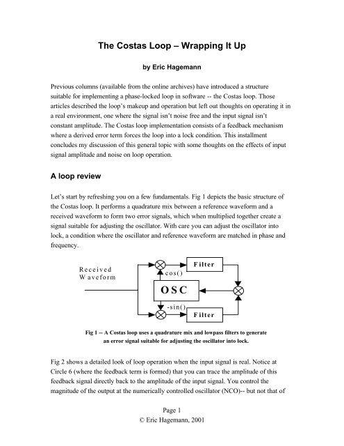
Let’s start by refreshing you on a few fundamentals. Fig 1 depicts the basic structure of
the Costas loop. It performs a quadrature mix between a reference waveform and a
received waveform to form two error signals, which when multiplied together create a
signal suitable for adjusting the oscillator. With care you can adjust the oscillator into
lock, a condition where the oscillator and reference waveform are matched in phase and
frequency.
Received
Waveform
cos()
OSC
-sin()
Filter
Filter
Fig 1 -- A Costas loop uses a quadrature mix and lowpass filters to generate
an error signal suitable for adjusting the oscillator into lock.
Fig 2 shows a detailed look of loop operation when the input signal is real. Notice at
Circle 6 (where the feedback term is formed) that you can trace the amplitude of this
feedback signal directly back to the amplitude of the input signal. You control the
magnitude of the output at the numerically controlled oscillator (NCO)-- but not that of
Page 1
© Eric Hagemann, 2001

the input. As you saw last time, the parameters α and β ration a feedback amount that
causes the loop to lock or not. Given insufficient feedback, the loop doesn’t converge;
with excess feedback, the loop diverges.
1
sin( wct + φ) * cos( wct
+ θ)
=
ct
sin −
2
1
sin( t + φ)
w c
2
[ sin(
2w
+ φ + θ)
+ ( φ θ ) ]
cos
NCO
−sin
1
sin( w ct
2
LPF
LPF
c t + φ) * ( −sin(
wct
+ θ))
= [ cos(
2w
+ φ + θ)
−cos(
φ −θ
) ]
[ −cos(
φ −θ
) ]
3
1
2
4
1
2
[ sin(
φ −θ
) ]
Page 2
© Eric Hagemann, 2001
1
1
error=
− sin
θ
4
4
6
5
( φ −θ
) cos(
φ −θ
) = − [ sin(
2(
φ − ) ) + sin(
0)
]
Fig 2 – Detailed look at A Costas loop with a real input signal showing the effect of down conversion
and formation of error or feed back signal
You’ll normally configure the loop to work with a fixed input amplitude, so what
happens when this constraint changes? In the design just described, the change in
amplitude carries directly through to the feedback term. If the input signal drops in
amplitude, the loop won’t converge; if the input signal increases, the loop might diverge.
A change in the input signal amplitude is equivalent to a change in α or β .
Amplitude immunity
Making loop operation independent of the input amplitude is desirable. Towards that goal
you can draw from two classes of solutions. The first approach fixes the input amplitude
through external means such as with an AGC (automatic gain control) circuit.
Alternately, you might also employ a hard limiter with a narrow bandpass filter.

A second set of solutions consists of making the loop itself tolerate amplitude variances.
A quick look at the multiplier at Circle 6 in Fig 2 reveals how that block functions as a
phase detector. Replacing this multiplier with an arctangent function achieves amplitude
independence. Given the quadrature components, the inverse tangent function returns the
instantaneous angle. The drawback to this solution consists of the computation cycles
required to implement the arctangent function. Most embedded processors or DSPs don’t
directly support this function in hardware, leaving the engineer to program a solution. For
an alternative more efficient that the functions you’ll find in a conventional compiler
library take a look at routines written around CORDIC (COrdinate Rotational DIgital
Computer) algorithms, whereby the rotation of unit vectors provides a way to accurately
compute trig functions.
Operation in noise
Because no real-world signal is noise-free, be sure to give consideration to operating the
loop in a noisy environment. The loop’s ability to function depends on how much noise
gets through to the adjustment of the NCO. The NCO update routines provide some
averaging and thus some immunity to noise, but the best method for controlling noise is
to appropriately set the bandwidth of the arm filters. Be sure to set these filters to
accomplish the desired acquisition range of the loop, but no wider. What’s the best
method of doing so?
You can employ almost any type filter including an IIR or FIR, but probably the simplest
and most suitable when tracking a single tone in noise is the single-pole IIR filter. It’s
also known as a recursive averager. The time domain equation is
Taking the z-transform produces
( )
Solving for the 3-dB point shows that
out = out*1 − α + in * α where 0< α < 1
f f f
α
( α )
1− 1−
Page 3
© Eric Hagemann, 2001
f
f z
.
( )
( − f )
2 2
1
⎡1+ 1−α 2
1 f − α ⎤
−
f
θ = cos ⎢ ⎥.
2π ⎢ 21 α ⎥
⎣ ⎦
Where θ is normalized frequency and α f is the critical design parameter -- it controls the
location of the pole. Be sure not to confuse it with the α used as the feedback coefficient

in the NCO update equations. Fig 3 shows the lowpass response of a 1-pole IIR filter
with α f = 0.1,
and Table 1 shows the calculated 3-dB bandwidths for several values of
α f .
Fig 3 -- Magnitude response for 1-pole IIR filter with α f = 0.1
α One Sided 3-dB Bandwidth
f
0.1 0.0167
0.2 0.035
0.3 0.057
Table 1 -- Calculated 3-dB bandwidths for one-pole IIR filters with differentα f
The arm filters control the amount of energy used in the feedback. As with the earlier
discussion on input-signal amplitude, attenuating the amount of energy that passes to the
phase detector inhibits the loop from operating outside a set frequency range, which the
Page 4
© Eric Hagemann, 2001

3-dB bandwidth of the IIR filters effectively set . Thus for the case of tracking a tone in
noise, you have a deterministic way of both setting the loop and in turn limiting the noise.
Fig 4 shows the lock-in range of a complex based Costas loop as limited by single-pole
IIR filters. The inner (blue) line shows the range when α f = 0.1.
The other two lines
show the effect of using α f = 0.2 and α f = 0.3 based filters. Contrast this operation with
the that of the complex Costas loop detailed last month where the lock range extended
across the entire frequency range (0.0 to 0.5, normalized).
Fig 4 -- Time to lock for a complex input Costas Loop implemented with 1-pole IIR filters using
α f =
0.1, 0.2, and 0.3
Wrapping it up
You now have in hand just about all the basics you need to work with a Costas loop --
loop construction, setting the feedback and adjusting the arm filters for optimum
operation. So the next time you’re looking for a PLL-like structure, give the Costas loop
a try!
Page 5
© Eric Hagemann, 2001

Author’s biography
Eric Hagemann (ehagemann@home.com) is an electrical engineer who has been
programming DSPs for fifteen years. When not writing code, he spends time with his
wife and two cats endlessly remodeling their house.
Page 6
© Eric Hagemann, 2001