M3M3 Partial Differential Equations
M3M3 Partial Differential Equations
M3M3 Partial Differential Equations

You also want an ePaper? Increase the reach of your titles
YUMPU automatically turns print PDFs into web optimized ePapers that Google loves.
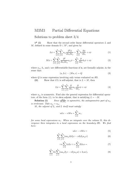
<strong>M3M3</strong> <strong>Partial</strong> <strong>Differential</strong> <strong>Equations</strong><br />
Solutions to problem sheet 3/4<br />
1* (i) Show that the second order linear differential operators L and<br />
M, defined in some domain Ω ⊂ R n , and given by<br />
n n ∂<br />
Lφ = aij<br />
i=1 j=1<br />
2 n φ ∂φ<br />
+ bi + cφ<br />
∂xi∂xj ∂xi<br />
i=1<br />
(1)<br />
n n ∂<br />
Mφ =<br />
2<br />
n ∂<br />
aijφ − biφ + cφ<br />
∂xi∂xj ∂xi<br />
(2)<br />
i=1 j=1<br />
where aij, bi, and c are differentiable functions of x, are formally adjoint, in the<br />
sense that:<br />
〈u, Lv〉 − 〈Mu, v〉 = Q (3)<br />
where Q is some expression involving only terms evaluated on ∂Ω.<br />
(ii) Show that if L is self-adjoint, that is L = M, then<br />
Lφ =<br />
n<br />
n<br />
i=1 j=1<br />
∂<br />
∂xi<br />
aij<br />
i=1<br />
∂<br />
φ + cφ (4)<br />
∂xj<br />
where aij is symmetric. Find also the general expression for differential operators,<br />
of the form (1), to be skew-adjoint, that is satisfying L = −M.<br />
∂<br />
Solution (i) Since<br />
2 φ<br />
is symmetric, the antisymmetric part of aij<br />
∂xi∂xj<br />
is irrelevant. Take aij = aji.<br />
M, the adjoint of L, and L itself must satisfy:<br />
uLv − vMu =<br />
n<br />
wi,<br />
for some local expressions wi. When we integrate over the volume Ω, this divergence<br />
then integrates to a local expression on the boundary ∂Ω. We find<br />
here:<br />
i=1<br />
n<br />
i=1 j=1<br />
+u<br />
i=1<br />
uLv − vMu = (5)<br />
n<br />
(uaij∂i∂jv − v∂i∂jaijv) (6)<br />
n<br />
bi∂iv + v<br />
i=1<br />
n<br />
∂ibiu = (7)<br />
i=1<br />
n n<br />
∂i( (uaij∂jv − v∂jaiju) + biuv), (8)<br />
j=1<br />
1
as required.<br />
(ii)Expanding Mu and equating with Lu, for self-adjointness, we find the<br />
coefficient of u gives<br />
n n ∂2 n aij ∂bi<br />
=<br />
∂xi∂xj ∂xi<br />
i=1 j=1<br />
and the coefficient of ∂iu gives<br />
i=1<br />
n ∂(aij + aji)<br />
= 2bi.<br />
∂xi<br />
i=1<br />
Since aij is symmetric, bi = n<br />
j=1<br />
∂aij<br />
∂xj<br />
. Expression (4) follows.<br />
2
2i Unseen and unexamined - Green’s functions for hyperbolic equations<br />
Show that if the Riemann (or Riemann-Green) function v(x, y; ξ, η) for a hyperbolic<br />
partial differential operator L, with adjoint L † ,<br />
is defined by<br />
then, for all x, y<br />
L = ∂2<br />
∂ ∂<br />
+ a(x, y) + b(x, y) + c(x, y) (9)<br />
∂x∂y ∂x ∂y<br />
L † v = 0, ξ > x, and η > y, (10)<br />
vy = av, x = ξ, (11)<br />
vx = bv, y = η (12)<br />
v = 0, ξ < x or η < y (13)<br />
v(ξ, η) = 1 (14)<br />
L † v = δ(x − ξ)δ(y − η). (15)<br />
Hint: write v(x, y) = w(x, y)H(ξ − x)H(η − y), where H is the Heaviside function,<br />
whose derivative is the δ-function, and w is a smooth function.<br />
Solution 2(i) Substitute v = w(x, y)H(ξ − x)H(η − y) into the adjoint<br />
pde<br />
Mv = δ(x − ξ)δ(y − η)<br />
. This gives terms in H(ξ − x)H(η − y), implying that w and hence v satisfy<br />
the pde if ξ > x and η > y. The conditions on ξ = x and η = y come from<br />
matching the coefficients of δ(ξ − x)H(η − y) and H(ξ − x)δ(η − y) respectively.<br />
The coefficient of δ(ξ − x)δ(η − y) gives the condition at the singular point<br />
ξ = x, η = y.<br />
(ii) Here v must satisfy<br />
vxy − ∂x<br />
v v<br />
− ∂y = 0,<br />
x + y x + y<br />
(16)<br />
vx = v/(x + y) y = η (17)<br />
vy = v/(x + y) x = ξ (18)<br />
v(ξ, η) = 1. (19)<br />
Clearly, taking v = (x + y)/(ξ + η) achieves this. Put L = ∂x∂y + 1/(x + y)(∂x +<br />
∂y), and L † is its adjoint. Integrate<br />
vLu − uL † v<br />
over the triangle Δ bounded by x = y, x = ξ, y = η. The integrand vanishes, as<br />
Lu = L † v = 0. However, it can also be written as a divergence<br />
∂x( 1<br />
2 (v∂yu − u∂yv) + uv/(x + y)) + ∂y( 1<br />
2 (v∂xu − u∂xv) + uv/(x + y)) = φx + ψy,<br />
3
say. Thus we get<br />
<br />
<br />
0 = φx + ψydxdy =<br />
Δ<br />
∂Δ<br />
φdy − ψdx.<br />
Now on x = y, we have u = 0, ux = f(x), and also uy = −f(x), for uxdx +<br />
uydy = du = 0. Integrating anticlockwise, along x = y, x = ξ, and y = η, we<br />
get, using the boundary conditions on u and on v,<br />
u(ξ, η) = 2<br />
ξ + η<br />
4<br />
η<br />
ξ<br />
xf(x)dx.
3* Using the maximum property for harmonic functions, prove the<br />
uniqueness of the solution to the Dirichlet problem for Poisson’s equation.<br />
Solution 3 The difference v between any two solutions of Poisson’s equation<br />
with the same Dirichlet data is a harmonic function which vanishes at the<br />
boundary. Being harmonic, this function takes its maximum (and minimum)<br />
values on the boundary; hence it vanishes everywhere.(4 marks)<br />
5
4i* Show that the solution of Helmholtz’ equation in 3 dimensions with<br />
Dirichlet boundary conditions:<br />
∇ 2 u + λu = f(x), x ∈ D (20)<br />
u = g(x), x ∈ ∂D, (21)<br />
is unique provided λ ≤ 0.<br />
ii With λ = k 2 > 0, a constant, find the radially symmetric solution<br />
u(r) of the Dirichlet BVP in the ball 0 < r < a, which satisfies:<br />
∇ 2 u + k 2 −2 d du<br />
u = r r2<br />
dr dr + k2u = 0, 0 < r < a, (22)<br />
u = 1<br />
, r = a, (23)<br />
4πa<br />
u − 1<br />
+ O(1), as r → 0. (24)<br />
4πr<br />
It will be helpful to put u(r) = v(r)/r and to find the ode satisfied by v(r).<br />
Hence show directly that the solution is not unique if k = π/a.<br />
Solution 4The difference between 2 solutions with the same Dirichlet data<br />
satisfies<br />
∇ 2 u + λu = 0, x ∈ D (25)<br />
u = 0, x ∈ ∂D. (26)<br />
Multiply the pde by u, and integrate over D. There is a vanishing boundary<br />
term, together with <br />
−|∇u|<br />
D<br />
2 + λu 2 dV.<br />
If u satisfies the pde, then this must vanish; however if λ < 0, and u is not<br />
identically zero, this is strictly negative. Hence u must be zero throughout D.<br />
For finite domains, this result is not the best possible; rather the solution is<br />
unique if λ < λ0, the smallest eigenvalue of −∇ 2 in D. So in the cube of side<br />
a, in 3 dimensions, λ0 = 3(π/a) 2 .<br />
ii In the ball of radius a, with λ = k 2 , the radially symmetric solution<br />
satisfies:<br />
−2 d du<br />
r r2<br />
dr dr + k2u = 0,<br />
Put u(r) = v(r)/r. So<br />
0 < r < a. (27)<br />
d 2 v<br />
dr 2 + k2 v = 0, 0 < r < a. (28)<br />
The b.c’s are v(0) = −1/(4π), so u is close to the free space Green’s function<br />
for the Laplace equation, as r → 0, and v(a) = 1/(4π), so<br />
v = −1/(4π) cos(kr) + A sin(kr) (29)<br />
6
with<br />
Thus<br />
v(a) = −1/(4π) cos(ka) + A sin(ka) = 1/(4π). (30)<br />
A = 1/(4π)<br />
cos(ka) + 1<br />
. (31)<br />
sin(ka)<br />
This obviously fails if k = π/a, when numerator and denominator both vanish;<br />
any value for A will do in this case.<br />
7
5 Show how the method of images may be used to solve the Dirichlet<br />
problem for Laplace’s equation in a two-dimensional wedge-shaped domain between<br />
two straight lines meeting at an angle α, for certain values of α.<br />
Hint - it is necessary to use multiple images. What values of α can be treated<br />
in this way?<br />
What image systems would be needed if instead we had Neumann conditions<br />
on one or both lines?<br />
Hence solve Laplace’s equation in the quarter-plane x > 0, y > 0, with<br />
Dirichlet conditions on the two axes and infinity:<br />
u = 1 on y = 0, 0 < x < 1 (32)<br />
u = 0 otherwise. (33)<br />
u → 0 as (x 2 + y 2 ) → ∞. (34)<br />
Solution 5In polar coordinates, with the origin at the vertex, if the free-space<br />
Green’s function is<br />
G0(r, θ, r ′ , θ ′ )<br />
we introduce images by repeated reflection in the two half-lines θ = 0, θ = α.<br />
These reflections are given by the two maps θ → −θ, and θ → 2α−θ respectively.<br />
These images give<br />
G(r, θ, r ′ , θ ′ ) = G0(r, θ, r ′ , θ ′ ) (35)<br />
−G0(r, −θ, r ′ , θ ′ ) − G0(r, 2α − θ, r ′ , θ ′ ) (36)<br />
+G0(r, 2α + θ, r ′ , θ ′ ) + G0(r, −2α + θ, r ′ , θ ′ ) . . . (37)<br />
The sum is periodic in θ with period 2α, corresponding to a double reflection,<br />
but also periodic with period 2π. Hence, if we are to ensure that the system of<br />
images is finite, without images in the original wedge, we find 2π must be an<br />
even integer multiple of α, α = π/n say. (3 marks)<br />
Neumann problems can be treated in the same way, but the sum must then<br />
be even under each reflection, so each term has a plus sign. (2 marks)<br />
In the quarter-plane, n = 2 and we need 3 images. The Green’s function we<br />
need here is<br />
G(x ′ , y ′ , z ′ ; x, y, 0) = 1<br />
4π (ln((x − x′ ) 2 + (y − y ′ ) 2 ) − ln((x + x ′ ) 2 + (y − y ′ ) 2 ) (38)<br />
− ln((x − x ′ ) 2 + (y + y ′ ) 2 ) + ln((x + x ′ ) 2 + (y + y ′ ) 2 )) (39)<br />
The first term is the free-space Green’s function, the second and third are its<br />
reflections under x → −x and y → −y, while the fourth term is the double<br />
reflection in both planes. The solution of the given problem is then<br />
Then, with<br />
u(x ′ , y ′ ) =<br />
∂G<br />
∂n |y=0 = y′<br />
π (<br />
1<br />
0<br />
∂G<br />
∂n (x′ , y ′ , x, 0)1dx, (40)<br />
1<br />
(x − x ′ ) 2 1<br />
−<br />
+ y ′2 (x + x ′ ) 2 ) (41)<br />
+ y ′2<br />
8
we get<br />
u(x ′ , y ′ ) = 1<br />
π (tan−1 y<br />
(<br />
′<br />
x ′ − 1 ) − 2 tan−1 ( y′<br />
x ′ ) + tan−1 y<br />
(<br />
′<br />
x ′ + 1 ))<br />
It can easily be checked geometrically that this satisfies the boundary conditions.<br />
(4 marks)<br />
9
6 Using the method of images, construct the Green’s function of the<br />
Neumann problem for Laplace’s equation in the half-space D = {(x, y, z) ∈ R 3 :<br />
z > 0}. Hence solve<br />
∇ 2 u = 0, x ∈ D (42)<br />
∂u<br />
∂z = 1 − x2 − y 2 , x 2 + y 2 < 1, z = 0 (43)<br />
∂u<br />
∂z = 0, x2 + y 2 > 1 z = 0, (44)<br />
and evaluate the resulting integral on the z-axis.<br />
− 1<br />
4π (<br />
Solution 6 The Neumann Green’s function is:<br />
1<br />
G(x, y, z; x ′ , y ′ , z ′ ) =<br />
(x − x ′ ) 2 + (y − y ′ ) 2 + (z − z ′ ) 2 +<br />
1<br />
(x − x ′ ) 2 + (y − y ′ ) 2 + (z + z ′ ) 2 )<br />
which is even in z. Integrate u∇ 2 G − G∇ 2 u over the upper half-space z ><br />
0, getting u(x ′ , y ′ , z ′ ). By the divergence theorem, this is equal to the surface<br />
integral ∞ ∞<br />
−∞<br />
−∞<br />
u ∂G ∂u<br />
− G<br />
∂n ∂n dxdy<br />
Now ∂/∂n = −∂/∂z, and ∂G/∂z|z=0 = 0. Thus<br />
∞ ∞<br />
Hence<br />
u(x ′ , y ′ , z ′ ) =<br />
−∞<br />
−∞<br />
u(0, 0, z ′ ∞ ∞<br />
) =<br />
−∞<br />
−∞<br />
= − 1<br />
2π 1<br />
4π θ=0<br />
1<br />
= −<br />
r=0<br />
1<br />
= −<br />
ρ=0<br />
G(x, y, 0; x ′ , y ′ , z ′ ) ∂u<br />
∂z<br />
G(x, y, 0; 0, 0, z ′ ) ∂u<br />
∂z<br />
r=0<br />
2<br />
√ r 2 + z ′2<br />
1<br />
√ r 2 + z ′2<br />
1<br />
2 ρ + z ′2<br />
rdr<br />
dρ<br />
rdrdθ<br />
= −[ ρ + z ′2 ] 1 0 = −( 1 + z ′2 − z ′ ).<br />
This plainly has the correct z’ derivative at z’=0.<br />
10<br />
dxdy.<br />
dxdy.
7 Solve the heat equation<br />
ut = uxx<br />
(45)<br />
with Neumann (insulating) boundary conditions ux = 0 on the ends of the<br />
interval [0, π], and initial condition<br />
u(x, 0) = δ(x − π/2), (46)<br />
in two different ways,<br />
(i) in terms of Green’s functions, using the method of images, and<br />
(ii) in terms of a Fourier cosine series, by separation of variables.<br />
Write these solutions in terms of two of the four theta functions, defined by:<br />
and<br />
θ4(s, q) =<br />
θ2(s, q) =<br />
∞<br />
n=−∞<br />
∞<br />
n=−∞<br />
(−1) n q n2<br />
cos(2ns), (47)<br />
q (n+1/2)2<br />
cos((2n + 1)s), (48)<br />
where q is chosen appropriately in each case. Hence, using the uniqueness<br />
theorem, derive the Jacobi imaginary transformation formula which relates θ2<br />
and θ4 for different values of q. Such formulae are important in the theory of<br />
elliptic functions, as these may be written as quotients of theta functions.<br />
See Lawden: Elliptic Functions and Applications, or other texts on elliptic<br />
functions, for further information.<br />
Solution 7 This heat equn can be solved in 2 ways. (i)By separation<br />
of variables: the solution must be a sum of terms like X(x)T (t), satisfying<br />
Tt/T = Xxx/X = constant. (49)<br />
Now X must be cos(2nx), n integer, to satisfy the Neumann boundary conditions<br />
at x = 0 and x = π, and we get<br />
At t = 0 we get<br />
u(x, t) =<br />
∞<br />
an cos(2nx) exp(−4n 2 t). (50)<br />
n=0<br />
δ(x) =<br />
∞<br />
(an cos(2nx)), (51)<br />
n=0<br />
so on multiplying by cos(2nx) or 1, and integrating, we find anπ/2 =<br />
cos(nπ) = (−1) n , and bn = 0, and a0π = 1.<br />
Thus<br />
u(x, t) = 1<br />
π<br />
∞<br />
n=−∞<br />
(−1) n cos(2n)x) exp(−4n 2 t) = 1<br />
11<br />
π θ4(x, t). (52)
(ii) Alternatively, using Green’s functions and the method of images, letting<br />
each image of the δ-function evolve into a copy of the free-space Green’s function<br />
centred at (2n + 1)π/2, we have:<br />
u(x, t) =<br />
=<br />
∞<br />
n=−∞<br />
∞<br />
n=−∞<br />
= exp(−x 2 /4t)<br />
= exp(−x 2 /4t)<br />
exp(−(x − (2n + 1)π/2) 2 /4t)/ √ 4πt<br />
exp(−x 2 + (2n + 1)πx − (2n + 1) 2 π 2 /4)/4t)/ √ 4πt<br />
∞<br />
n=−∞<br />
∞<br />
n=−∞<br />
exp(<br />
(2n + 1)xπ<br />
) exp(−(n +<br />
4t<br />
1<br />
2 )2π 2 /t))/ √ 4πt<br />
cosh(<br />
= exp(−x 2 /4t)/ √ 4πt θ2( −ixπ<br />
,<br />
4t<br />
π2<br />
4t ),<br />
(2n + 1)xπ<br />
) exp(−(n +<br />
4t<br />
1<br />
2 )2π 2 /t))/ √ 4πt<br />
where we have used the evenness of cosh to symmetrise the sum in the last<br />
step. Since these 2 expressions solve the same equation with the same boundary<br />
conditions, they must be equal by the uniqueness theorem. This gives the<br />
transformation formula required, which relates values of θ3 for large and small<br />
values of its second argument.<br />
12
8* Solve<br />
ut = uxx<br />
i on the line with the initial condition:<br />
(53)<br />
u(x, 0) = 1<br />
,<br />
2a<br />
|x| < a, (54)<br />
u(x, 0) = 0, |x| > a, (55)<br />
and describe the limit a → 0;<br />
ii and, on the half-line x > 0, with the boundary and initial conditions:<br />
u(x, 0) = 0, (56)<br />
u(0, t) = 1. (57)<br />
Solution 8* (i) As in notes, using the Green’s function G(x, t) =<br />
1<br />
√ 4πt exp(−x 2 /(4t)), we get<br />
∞<br />
a<br />
1 1<br />
√<br />
4πt −a<br />
(a−x)<br />
1 1<br />
√<br />
2a 4πt<br />
u(x, t) = (58)<br />
u(x<br />
−∞<br />
′ , 0)G(x − x ′ , t)dx ′ = (59)<br />
2a exp(−(x − x′ ) 2 /4t)dx ′ = (60)<br />
exp(−(x<br />
−(x+a)<br />
′ ) 2 /4t)dx ′ = (61)<br />
1<br />
2a √ π (erf((a − x)/ (4t)) − erf(−(a + x)/ (4t))), (62)<br />
where erf(x) = 2/ √ π x<br />
0 exp(−t2 )dt. As a → 0, u(x, t) → G(x, t).<br />
(ii) Here we need G(x, x ′ , t) = 1 √ (exp(−(x−x<br />
4πt ′ ) 2 /(4t))−(exp(−(x+<br />
x ′ ) 2 /(4t)), so that:<br />
u(x, t) =<br />
∞<br />
0<br />
t<br />
0<br />
u(x ′ , 0)G(x − x ′ , t)dx ′ t<br />
− u(0, t<br />
0<br />
′ ) ∂G(x, t − t′ )<br />
=<br />
∂x<br />
(63)<br />
x<br />
(t − t ′ x2<br />
exp(−<br />
) 3/2 4(t − t ′ ) )dt′ . (64)<br />
1<br />
√ 4π<br />
Now put τ = x/(2 √ t − t ′ ); the result becomes:<br />
∞<br />
2<br />
√ exp(−τ<br />
π 2 )dτ,<br />
that is<br />
τ=x/(2 √ t)<br />
u = (1 − erf( x<br />
2 √ t )).<br />
13
9 Consider the nonlinear diffusion equation<br />
ut = u n uxx, (65)<br />
in the domain t > 0, 0 < x < 1, with the initial and boundary conditions:<br />
u(x, 0) = f(x), (66)<br />
u(0, t) = u(1, t) = 0. (67)<br />
If n is a positive integer, and f(x) is square-integrable, show that if<br />
1<br />
E = u 2 dx, (68)<br />
0<br />
then<br />
dE<br />
≤ 0,<br />
dt<br />
(69)<br />
provided that n is even. Discuss why the problem may not be well-posed for<br />
odd n; show that E(t) can increase in this case. Discuss the generalisation to<br />
more than one space dimension.<br />
Solution 9 Multiply the equation by 2u, so that:<br />
(u 2 )t = 2u n+1 uxx<br />
Hence on integrating by parts, over the interval 0 < x < 1,<br />
dE<br />
dt<br />
(70)<br />
1<br />
= −2(n + 1) u n u 2 xdx. (71)<br />
If n is even, the rhs is negative, and E is a decreasing function of time. However<br />
the sign of the integrand on the right is not definite for odd n. In the latter<br />
case, E may increase if u is somewhere negative; indeed, linearising about some<br />
negative constant u0, with u = u0+ɛu1, where 0 < ɛ ≪ 1, we see that u1satisfies<br />
a backwards heat equation, which is ill-posed. We would expect solutions to<br />
grow without bound in this case, in any region where u is negative. Analogous<br />
results can be obtained using the divergence theorem in more than one space<br />
dimension.<br />
14<br />
0
10 Self-similar solutions Find m, n such that the ansatz u(x, t) =<br />
t m f(xt n ) satisfies Burger’s equation:<br />
ut + uux = uxx. (72)<br />
Find the ordinary differential equation satisfied by f, and hence solve Burger’s<br />
equation with<br />
u(0, t) = −2/(πt) 1/2<br />
(73)<br />
u → 0, x → ∞. (74)<br />
Solution 10 Put ξ = xt n , u = t m f(xt n ), in the equation; we get:<br />
Rearranging,<br />
mt m−1 f + nxt m+n−1 f ′ + t 2m+n ff ′ = t m+2n f ′′ . (75)<br />
mf + nξf ′ + t m+n+1 ff ′ = t 2n+1 f ′′ . (76)<br />
Equate coefficients of t to get n = m = −1/2.<br />
Then<br />
Integrating, with f → 0 as x → ∞:<br />
Put f = −2ψ ′ /ψ so that<br />
u(x, t) = f(x/t 1/2 )/t 1/2 . (77)<br />
f ′′ − ff ′ + 1/2ξf ′ + 1/2f = 0 (78)<br />
f ′ − f 2 /2 + 1/2ξf = 0. (79)<br />
ψ ′′ + 1/2ξψ ′ = 0, (80)<br />
giving ψ ′ = exp(−ξ 2 /4). The constant of integration is irrelevant here. Hence<br />
Thus we get<br />
ψ = √ πerf(ξ/2) + A. (81)<br />
exp(−ξ<br />
f = −2<br />
2 /4)<br />
√ . (82)<br />
πerf(ξ/2) + A<br />
At ξ = 0, this reduces, with the condition on x = 0, to f = −2/A = −2/ √ π.<br />
Finally, we obtain<br />
u = − 2 exp(−x<br />
√<br />
t<br />
2 /(4t))<br />
√ √ . (83)<br />
πerf(ξ/2) + π<br />
15


![Time Series (S8) 2012/2013 Coursework I: SOLUTIONS [1] (a) cov ...](https://img.yumpu.com/46239625/1/184x260/time-series-s8-2012-2013-coursework-i-solutions-1-a-cov-.jpg?quality=85)