Computing Extremal Quasiconformal Maps - Technion
Computing Extremal Quasiconformal Maps - Technion
Computing Extremal Quasiconformal Maps - Technion

You also want an ePaper? Increase the reach of your titles
YUMPU automatically turns print PDFs into web optimized ePapers that Google loves.
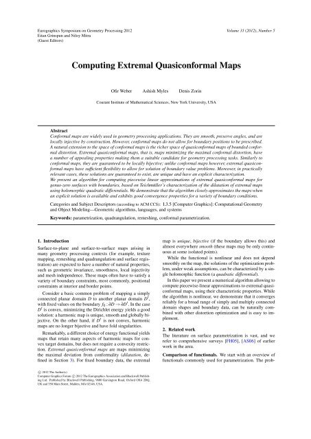
Eurographics Symposium on Geometry Processing 2012<br />
Eitan Grinspun and Niloy Mitra<br />
(Guest Editors)<br />
<strong>Computing</strong> <strong>Extremal</strong> <strong>Quasiconformal</strong> <strong>Maps</strong><br />
Ofir Weber Ashish Myles Denis Zorin<br />
Courant Institute of Mathematical Sciences, New York University, USA<br />
Volume 31 (2012), Number 5<br />
Abstract<br />
Conformal maps are widely used in geometry processing applications. They are smooth, preserve angles, and are<br />
locally injective by construction. However, conformal maps do not allow for boundary positions to be prescribed.<br />
A natural extension to the space of conformal maps is the richer space of quasiconformal maps of bounded conformal<br />
distortion. <strong>Extremal</strong> quasiconformal maps, that is, maps minimizing the maximal conformal distortion, have<br />
a number of appealing properties making them a suitable candidate for geometry processing tasks. Similarly to<br />
conformal maps, they are guaranteed to be locally bijective; unlike conformal maps however, extremal quasiconformal<br />
maps have sufficient flexibility to allow for solution of boundary value problems. Moreover, in practically<br />
relevant cases, these solutions are guaranteed to exist, are unique and have an explicit characterization.<br />
We present an algorithm for computing piecewise linear approximations of extremal quasiconformal maps for<br />
genus-zero surfaces with boundaries, based on Teichmüller’s characterization of the dilatation of extremal maps<br />
using holomorphic quadratic differentials. We demonstrate that the algorithm closely approximates the maps when<br />
an explicit solution is available and exhibits good convergence properties for a variety of boundary conditions.<br />
Categories and Subject Descriptors (according to ACM CCS): I.3.5 [Computer Graphics]: Computational Geometry<br />
and Object Modeling—Geometric algorithms, languages, and systems<br />
Keywords: parametrization, quadrangulation, remeshing, conformal parametrization.<br />
1. Introduction<br />
Surface-to-plane and surface-to-surface maps arising in<br />
many geometry processing contexts (for example, texture<br />
mapping, remeshing and quadrangulation and surface registration)<br />
are expected to have a number of natural properties,<br />
such as geometric invariance, smoothness, local injectivity<br />
and mesh independence. These maps often have to satisfy a<br />
variety of boundary constraints, most commonly, positional<br />
constraints at interior and border points.<br />
Consider a basic common problem of mapping a simply<br />
connected planar domain D to another planar domain D ′ ,<br />
with fixed values on the boundary f0 : ∂D → ∂D ′ . In the case<br />
D ′ is convex, minimizing the Dirichlet energy yields a good<br />
solution: a harmonic map is unique, smooth and globally bijective.<br />
On the other hand, if D ′ is not convex, harmonic<br />
maps are no longer bijective and have fold singularities.<br />
Remarkably, a different choice of energy functional yields<br />
maps that retain many aspects of harmonic maps for convex<br />
target domains, but does not require a convexity restriction.<br />
<strong>Extremal</strong> quasiconformal maps are maps minimizing<br />
the maximal deviation from conformality (dilatation, defined<br />
in Section 3). For fixed boundary data, the extremal<br />
c○ 2012 The Author(s)<br />
Computer Graphics Forum c○ 2012 The Eurographics Association and Blackwell Publishing<br />
Ltd. Published by Blackwell Publishing, 9600 Garsington Road, Oxford OX4 2DQ,<br />
UK and 350 Main Street, Malden, MA 02148, USA.<br />
map is unique, bijective (if the boundary allows this) and<br />
almost everywhere smooth (these maps may be only continuous<br />
at some isolated points).<br />
While the functional is nonlinear and does not depend<br />
smoothly on the map, the solutions of the optimization problem,<br />
under weak assumptions, can be characterized by a single<br />
holomorphic function (a quadratic differential).<br />
In this paper we present a numerical algorithm allowing to<br />
compute piecewise-linear approximations to extremal quasiconformal<br />
maps, using their characteristic properties. While<br />
the algorithm is nonlinear, we demonstrate that it converges<br />
reliably for a broad range of simply and multiply connected<br />
domain shapes and boundary data, can be naturally combined<br />
with other distortion optimization and is easy to implement.<br />
2. Related work<br />
The literature on surface parametrization is vast, and we<br />
refer to comprehensive surveys [FH05], [AS06] of earlier<br />
work in the area.<br />
Comparison of functionals. We start with an overview of<br />
functionals commonly used for parametrization. The prob
O. Weber & A. Myles & D. Zorin / <strong>Computing</strong> <strong>Extremal</strong> <strong>Quasiconformal</strong> <strong>Maps</strong><br />
functional/PDE<br />
harmonic<br />
LIN BC FLD UNI BIJ<br />
[Tut63, Flo97]<br />
[DMA02,<br />
+ + finite + convex<br />
LPRM02]<br />
conformal<br />
[GY03, KSS06,<br />
BGB08,SSP08]<br />
- - N/A + any<br />
least-stretch<br />
[SSGH01]<br />
MIPS<br />
[HG99]<br />
elasticity<br />
[Bal81, CLR04]<br />
-<br />
-<br />
-<br />
+<br />
+<br />
+<br />
∞<br />
∞<br />
∞<br />
-<br />
-<br />
-<br />
any<br />
any<br />
any<br />
extremal q.c. - + finite + any<br />
Table 1: Properties of smooth parametrization functionals.<br />
lem of defining a mapping from a surface to the plane or<br />
between surfaces has two principal aspects: a smooth definition<br />
(typically an energy measuring distortion) and corresponding<br />
discrete energy. The choice of underlying smooth<br />
energy is essential, as the flaws in this choice cannot be fully<br />
resolved by a good choice of discretization; in the limit of<br />
fine meshes the behaviors are likely to be similar.<br />
Many energies and PDEs were proposed for parametrization<br />
and related problems. The most important ones are summarized<br />
in Table 1. We focus on several important properties,<br />
linearity of defining equations (LIN), whether mappings<br />
in this class can satisfy arbitrary boundary conditions (BC),<br />
whether the solution is unique (UNI) and for which domains<br />
it is bijective (BIJ).<br />
An additional property, particularly important for nonlinear<br />
functionals, is their behavior for maps with folds (column<br />
FLD). We observe that all functionals ensuring bijectivity<br />
on arbitrary domains typically achieve this by fast growth to<br />
infinity as the mapping develops folds. As a consequence,<br />
the functionals are nonlinear, and require a starting point<br />
for optimization. This combination of properties results in<br />
a fundamental problem: a bijective map is needed to initialize<br />
the optimization, as the functional is infinite for any nonbijective<br />
initial map.<br />
These observations highlight the unique properties of extremal<br />
quasiconformal maps: the functional remains finite on<br />
folds, and, under relatively weak assumptions on boundary<br />
data, has a unique minimizer.<br />
MIPS parametrization introduced in [HG99] is of particular<br />
interest, as it is an integral of a symmetric form of a<br />
dilatation measure and is closely related to extremal quasiconformal<br />
maps, as discussed in Section 3.<br />
Constrained parametrization. Methods for constrained<br />
parametrization were proposed in [Lév01, ESG01, KSG03,<br />
KGG05]. The method of [Lév01] optimizes Dirichlet energy<br />
and imposes pointwise position and gradient constraints<br />
with penalty terms, without attempting to guarantee bijectivity.<br />
Other techniques [ESG01, KSG03, KGG05] take an<br />
approach that can be characterized as achieving bijectivity<br />
first, possibly with mesh refinement, and without attempt-<br />
ing to approximate a smooth functional, and then smoothing<br />
the resulting parametrization while enforcing the bijectivity<br />
constraint. The problem of this class of approaches is<br />
that the optimal constrained solution is likely to be on the<br />
boundary of the feasible domain, which negatively affects<br />
the parametrization quality.<br />
<strong>Quasiconformal</strong> maps. The work most closely related to<br />
ours is the work on quasiconformal maps and Beltrami<br />
flows. In [ZRS05], quasi-harmonic maps are considered<br />
(harmonic maps in a user-specified metric). One can view<br />
these as approximations to quasi-conformal maps.<br />
<strong>Quasiconformal</strong> maps, typically on disk domains, were<br />
computed by solving the Beltrami equation with prescribed<br />
Beltrami coefficient, e.g. in [Dar93]. [ZLYG09] proposes<br />
a method for computing quasiconformal maps from Beltrami<br />
coefficients on general multiply connected domains.<br />
In [LWT ∗ 10], holomorphic Beltrami flow is introduced for<br />
shape registration. Beltrami coefficient is used as a shape<br />
representation and two shapes are matched by evolving the<br />
Beltrami coefficient so that the landmarks are matched and<br />
the L 2 norm of the Beltrami coefficient, is minimized.<br />
[LKF12] demonstrates that in the special case of four<br />
point constraints and periodicity conditions, an extremal<br />
quasiconformal map from the complex plane to itself has<br />
closed form.<br />
In mathematics, the theory of Teichmüller maps and<br />
spaces has a long history, starting with the work of Grötzsch<br />
[Grö30], with key ideas introduced by Teichmüller [Tei40,<br />
Tei43] and it remains an active area of research. Many fundamental<br />
questions were settled by Ahlfors [Ahl53]. A number<br />
of books, e.g., [Ahl66, GL00] provide a comprehensive<br />
introduction to the subject.<br />
Teichmüller spaces, i.e. spaces of conformal equivalence<br />
classes of surfaces, were introduced to graphics and vision<br />
literature in [SM04, JZLG09], and further developed<br />
in [JZDG09,WDC ∗ 09]. The extremal dilatation of quasiconformal<br />
maps define a metric on these spaces, but this metric<br />
was not used in this work.<br />
The interest in quasiconformal maps is to great extent<br />
motivated by the attractive properties of conformal maps,<br />
for which a number of high-quality computational algorithms<br />
were proposed [GY03,BGB08,KSS06,SSP08]. ABF<br />
[SdS01] can also be viewed as a conformal map approximation.<br />
Last three methods (when the optimization converge<br />
to a valid solution) guarantee bijectivity of discrete<br />
maps, these algorithms allow for free boundaries, or curvature<br />
constraints on the boundary, but not positional constraints.<br />
ARAP [LZX ∗ 08] minimizes deviation from isometry.<br />
Global parametrization methods deal with surfaces of<br />
higher genus, and correspond to flat metrics with cones, e.g.,<br />
recent feature aligned methods [RLL ∗ 06, KNP07, BZK09].<br />
In the context of bijective maps, [BZK09] is of particular<br />
interest, proposing iterative stiffening as a way to eliminate<br />
foldovers inherent to harmonic-like parametrizations with<br />
constraints.<br />
c○ 2012 The Author(s)<br />
c○ 2012 The Eurographics Association and Blackwell Publishing Ltd.
O. Weber & A. Myles & D. Zorin / <strong>Computing</strong> <strong>Extremal</strong> <strong>Quasiconformal</strong> <strong>Maps</strong><br />
3. Background<br />
In our exposition we primarily focus on maps from plane<br />
to plane. Due to conformal invariance, all concepts can be<br />
easily generalized to surfaces of genus zero by mapping the<br />
surface conformally to the plane. However, as we briefly explain<br />
in Section 6 all concepts and the algorithm can be extended<br />
to surfaces of arbitrary genus.<br />
We will use complex coordinates in the plane, z = x + iy.<br />
For an arbitrary (not necessarily holomorphic) differentiable<br />
function f (z), the complex derivatives are fz = 1 2 ( fx − i fy)<br />
and f¯z = 1 2 ( fx + i fy). We assume that for all maps these<br />
derivatives are defined almost everywhere, and are squareintegrable.<br />
For each complex number z we define a ma-<br />
Re(z) −Im(z)<br />
trix A(z) =<br />
and a vector v(w) =<br />
Im(z) Re(z)<br />
(Re(w),Im(w)) ⊤ , so that zw corresponds to A(z)v(w).<br />
Dilatation and quasiconformal maps. The little dilatation<br />
of a differentiable map f at z is defined as<br />
<br />
<br />
k(z) = <br />
f¯z<br />
<br />
<br />
<br />
fz<br />
<br />
(1)<br />
It is related to the ratio K of singular values of the Jacobian<br />
of f (large dilatation) by K = 1+k<br />
1−k . A map f : D → D′ is<br />
quasiconformal if k(z) ≤ k for some k almost everywhere in<br />
D. In this case, k( f ) = supk(z) is the maximal dilatation of<br />
the map. The dilatation k has the following important properties:<br />
• 0 ≤ k < 1 for orientation-preserving maps, and 1 ≤ k ≤ ∞<br />
for orientation reversing maps.<br />
• for a conformal map k = 0 and a conformal map composed<br />
with reflection k = ∞.<br />
An advantage of considering k instead of K is that k varies<br />
continuously as the sign of the determinant of the Jacobian<br />
of f changes on folds, while K has a singularity (cf. comparison<br />
of functionals in Section (2)).<br />
For a quasiconformal map with fz = 0 almost everywhere,<br />
µ = f¯z/ fz is called the complex Beltrami coefficient, (Figure<br />
1) and the equation<br />
is the Beltrami equation.<br />
1–k<br />
f¯z = µ fz<br />
θ<br />
1+k<br />
θ = 1<br />
arg μ<br />
2<br />
Figure 1: Geometric meaning of the complex Beltrami coefficient<br />
µ = ke 2iθ .<br />
If g and h are conformal, then h ◦ f ◦ g is quasiconformal<br />
with the same dilatation k as f . The simplest map with dilatation<br />
k is an affine stretch Ak along the two coordinate<br />
c○ 2012 The Author(s)<br />
c○ 2012 The Eurographics Association and Blackwell Publishing Ltd.<br />
(2)<br />
axes by 1 + k and 1 − k respectively; this yields a family of<br />
quasiconformal maps with constant dilatation k(z) = k, of<br />
the form<br />
f = h ◦ Ak ◦ g. (3)<br />
This simple example of quasiconformal maps plays an important<br />
role in the theory of extremal quasiconformal maps.<br />
<strong>Extremal</strong> quasiconformal maps. Suppose a quasiconformal<br />
map h : D → D ′ maps a (possibly multiply connected)<br />
domain D to D ′ . Let B be a subset of the boundary of D, and<br />
consider the set QB of all quasiconformal maps f that agree<br />
with h on B and are homotopic to h (Figure 2). In the set QB<br />
there is a map f ext , with k( f ext ) ≤ k( f ) for any f . The map<br />
f ext is called the extremal quasiconformal map.<br />
A<br />
B<br />
Figure 2: Examples of nonhomotopic maps with the same<br />
boundary data on ring domain; the left plot represents identity;<br />
note that the path AB connecting two boundary points<br />
on the right, cannot be continuously deformed to the spiral<br />
path AB on the left, while keeping the boundary fixed. An<br />
extremal quasiconformal map is unique for each homotopy<br />
class under assumptions of Proposition 2.<br />
2π<br />
π<br />
0<br />
A<br />
B<br />
zero derivative<br />
Figure 3: Left: A non-Teichmüller extremal map of the disk<br />
to itself. The image of the polar coordinate grid is shown.<br />
Right: the boundary values of the map on the circle in angular<br />
coordinates.<br />
For a broad range of practically relevant boundary conditions,<br />
extremal quasiconformal maps have a very specific<br />
local structure that can be described in terms of a pair of conformal<br />
maps, and a global structure that can be characterized<br />
by a quadratic differential.<br />
π<br />
2π
O. Weber & A. Myles & D. Zorin / <strong>Computing</strong> <strong>Extremal</strong> <strong>Quasiconformal</strong> <strong>Maps</strong><br />
Teichmüller maps. Locally in a neighborhood of every<br />
point (excluding zeros of gz), a Teichmüller map has the form<br />
(3): h◦Ak ◦g, for a choice of conformal maps h(w) and g(z),<br />
where w denotes the complex coordinate on the intermediate<br />
domain Ak acts on.<br />
A simple calculation leads to the following lemma:<br />
Lemma 1 For a map f = h ◦ Ak ◦ g, where h and g are conformal,<br />
and Ak is a stretch with dilatation k, the Beltrami<br />
coefficient has the form<br />
where φ = (gz) 2 .<br />
f¯z<br />
fz<br />
= k ¯φ<br />
|φ|<br />
Proof By Cauchy-Riemann equations, h ¯w = 0, and g¯z = 0;<br />
similarly, for the anti-conformal map ¯g, ¯gz = 0. Observe that<br />
the affine map Ak(w) in complex form can be written as<br />
Ak(w) = w + k ¯w. For this reason, fz = hw(gz + k ¯gz) = hwgz,<br />
and f¯z = hw(g¯z +k ¯g¯z) = khw ¯g¯z (because g is conformal, g¯z =<br />
0 and ¯gz = 0). We observe that f¯z/ fz = k ¯g¯z/gz = kgz 2 /|g 2 z |,<br />
as ¯g¯z = gz.<br />
source<br />
Ak stretch h<br />
target<br />
g<br />
Figure 4: Locally, a Teichmüller map can be decomposed<br />
into two conformal maps and an affine transform.<br />
The quantity φ = g 2 z is called the quadratic differential<br />
of f . Geometrically, the quadratic differential can be interpreted,<br />
up to a scale, as the traceless part of the metric tensor<br />
M = J[ f ] ⊤ J[ f ] of the map f , where J[ f ] is the Jacobian matrix.<br />
More specifically, the singular vectors of A(φ(z)) determine<br />
the stretch directions of f at z.<br />
More generally, a quadratic differential on a domain with<br />
a complex coordinate z is defined by a holomorphic function<br />
φ(z), which depends on the choice of the coordinate system.<br />
If w is a different choice of complex coordinates on the domain,<br />
then φ w (w)w 2 z = φ(z). This change-of-coordinates rule<br />
also allows to define a quadratic differential on a Riemann<br />
surface by a set of holomorphic functions on local charts.<br />
Definition 1 On a planar domain D, a map f is called a Teichmüller<br />
map, if it is quasiconformal with Beltrami coefficient<br />
of the form<br />
µ(z) = k φ(z)<br />
|φ(z)|<br />
where φ is a holomorphic function and k is a constant dilatation,<br />
everywhere where φ = 0.<br />
(4)<br />
Observe that the definition is invariant with respect to composition<br />
with conformal maps on either side. While postcomposition<br />
does not change the Beltrami coefficient, precomposition<br />
results in a change in φ but not in k.<br />
Unlike the definition of extremal quasiconformal maps,<br />
involving minimization of a nonsmooth and nonlinear functional,<br />
Teichmüller maps are much more amenable to computation,<br />
thanks to explicit form of the Beltrami coefficient.<br />
Fortunately, in most cases, an extremal map is a Teichmüller<br />
map and it is unique. In particular, the following proposition<br />
can be obtained from a sufficient condition for Teichmüller<br />
map existence for disks [Rei02] and conformal mapping<br />
properties:<br />
Proposition 2 For two simply connected bounded domains<br />
D and D ′ with piecewise smooth boundaries forming nondegenerate<br />
corners; suppose h : ∂D → ∂D ′ is a function with<br />
continuous nonvanishing bounded derivative and almost everywhere<br />
defined second derivative. Then in every homotopy<br />
class of maps f satisfying f | ∂D = h, there is a unique<br />
extremal Teichmüller map f with bounded L1-norm of the<br />
quadratic differential φ.<br />
As illustrated in Figure 3, the conditions on h in proposition<br />
2 are essential. The quasiconformal map of the disk<br />
to itself shown in this image is known to be extremal for its<br />
boundary values [Rei02]. The map in the image is obtained<br />
as f2 ◦ g ◦ f1, where f1(z) = i(1 + z)/(1 − z) maps the disk<br />
to the upper half-plane, f2 is its inverse, and g(z) = |z|z, and<br />
can be easily shown not to be a Teichmüller map.<br />
A similar statement appears to hold for multiply connected<br />
domains [Gar], but we were unable to locate a published<br />
proof. These theorems extend immediately to surfaces<br />
of genus zero with boundary, and also hold for maps between<br />
surfaces of arbitrary finite genus. In this paper, we focus on<br />
genus zero.<br />
Proposition 2 is the foundation of our approach for the<br />
computation of extremal maps. For these types of boundary<br />
data, it is sufficient to find a map with holomorphic quadratic<br />
differential and constant dilatation.<br />
Quadratic differential structure. Before discussing the algorithm<br />
we briefly mention the local structure of quadratic<br />
differentials near its zeros and poles. The quadratic differentials<br />
of Teichmüller maps have only simple poles, and generically<br />
zeros of order 1. The trajectories of quadratic differentials<br />
are integral lines of the fields of singular directions<br />
of A(φ(z)). These directions change rapidly near zeros and<br />
poles, as can be seen in Figure 5. While poles of quadratic<br />
differentials always remain on the boundaries, zeros spontaneously<br />
appear in the interior or on the boundary (Figure 9).<br />
4. Algorithm<br />
Overview. Given a boundary function fb and an initial (not<br />
necessarily bijective) map satisfying boundary conditions,<br />
we compute a piecewise-linear approximation to a Teichmüller<br />
map minimizing a discretization of the least-squares<br />
Beltrami (LSB) energy:<br />
<br />
ELSB =<br />
D<br />
<br />
<br />
<br />
f¯z − k ¯φ<br />
|φ| fz<br />
<br />
2<br />
<br />
dA (5)<br />
c○ 2012 The Author(s)<br />
c○ 2012 The Eurographics Association and Blackwell Publishing Ltd.
pole zero<br />
O. Weber & A. Myles & D. Zorin / <strong>Computing</strong> <strong>Extremal</strong> <strong>Quasiconformal</strong> <strong>Maps</strong><br />
Figure 5: Behavior of a Teichmüller map near poles and<br />
zeros of a quadratic differential.<br />
with f , φ and k are unknowns, and the constraints φ¯z = 0 (i.e.<br />
φ is holomorphic) and f | ∂D = fb are applied.<br />
By Teichmüller uniqueness and existence, this energy has<br />
a single global minimum with value zero, in the homotopy<br />
class of its initial point. We note that the energy is not convex.<br />
However, we have observed (see Section 5) that it consistently<br />
converges starting from a variety of arbitrary initial<br />
starting points.<br />
There are two essential conditions defining the Teichmüller<br />
map that need to be converted to a discrete form: (1)<br />
the quadratic differential defining the map has to be holomorphic<br />
(2) the dilatation k has to be constant. Note however<br />
that a discrete piecewise-linear map cannot, in general,<br />
achieve a perfectly constant k, and as a consequence, zero<br />
LSB energy. This is also the case for discrete conformal<br />
maps, for which k should be constant zero, but deviates from<br />
zero significantly (this is demonstrated in Figure 6).<br />
0.1<br />
0<br />
40<br />
20<br />
0<br />
0 0.5<br />
Figure 6: The distribution of dilatation values for a conformal<br />
map computed using the method of [SSP08]. Note<br />
that although the method produces a high-quality conformal<br />
map, the dilatations on triangles may be far from zero.<br />
4.1. Discretization<br />
We represent f as a piecewise-linear map defined by values<br />
at vertices of the original mesh. The complex derivatives f¯z<br />
and fz are naturally defined per triangle. If ei,ej,ek, are edge<br />
vectors of a triangle T with opposite vertices (i, j,k), the gra-<br />
fiti+ f jt j+ fktk<br />
dient of piecewise-linear f is given by , where<br />
2AT<br />
AT is the triangle area, ti = e ⊥ i , and fi are values at the vertices.<br />
It immediately follows that per-triangle derivatives are<br />
c○ 2012 The Author(s)<br />
c○ 2012 The Eurographics Association and Blackwell Publishing Ltd.<br />
given by<br />
fz = 1 <br />
fi<br />
4AT<br />
¯ti + f j ¯<br />
f¯z = 1<br />
4AT<br />
t j + fk ¯ tk<br />
<br />
,<br />
<br />
fiti + f jt j + fktk<br />
where ti = t x i + it y<br />
i is the complex form of the vectors ti =<br />
(t x i ,t y<br />
i ).<br />
Discretization of quadratic differentials. The holomorphic<br />
condition on the quadratic differential φ, φ¯z = 0 can<br />
be discretized in a similar manner if the quadratic differential<br />
values are defined per vertex. However, this definition<br />
does not naturally reflect the relation between f and φ.<br />
Equation (2) suggests that the Beltrami coefficient µ, and,<br />
as a consequence, the quadratic differential φ, is most naturally<br />
defined in a way consistent with f¯z and fz, i.e., per<br />
triangle. If we use notation ¯φ = vx + ivy for the components<br />
of the conjugate of the quadratic differential, then the holomorphic<br />
condition φ¯z = 0 can be written more explicitly as<br />
∂xvx +∂yvy = 0 and ∂yvx −∂yvy = 0, with two equations corresponding<br />
to equating real and imaginary parts of φ¯z to zero.<br />
If we regard the pair (vx,vy) as components of a 1-form<br />
h = vxdx + vydy, then dh = (∂yvx − ∂xvy)dx ∧ dy. Similarly,<br />
as the Hodge star acts on 2D 1-form components as a 90degree<br />
rotation, we get for the co-boundary operator δh =<br />
∗d ∗ h = ∂xvx + ∂yvy. Thus, we conclude that the 1-form h =<br />
Re(φ)dx − Im(φ)dy is harmonic:<br />
(6)<br />
dh = 0, δh = 0. (7)<br />
If we regard v = (vx,vy) as a vector field, this pair of equations<br />
correspond to zero curl and divergence of v. This observation<br />
suggests a standard per-edge discretization, with real<br />
scalars associated with edges, and standard discretizations<br />
of d and δ operators. Let hi j be the value of the harmonic<br />
1-form on the edge ei j. For convenience, we use notation<br />
h ji = −hi j.<br />
For a triangle T = (i, j,k), let ri j = e ⊥ j − e ⊥ i , and define<br />
r jk and rki by cyclic permutation. We represent the vectors<br />
r = (rx,ry) in complex form r = rx + iry.<br />
Then the per-triangle quadratic differential values are defined<br />
by<br />
φT = 1 <br />
hi jri j + h jkr jk + hkirki . (8)<br />
6AT<br />
Discrete energy and constraints. To summarize, the energy<br />
(5) is discretized using per-vertex complex variables fi<br />
to represent the map, a single scalar k for the constant dilatation<br />
and a real harmonic vector 1-form represented by<br />
per-edge values hi j. The energy is given by<br />
E d LSB = ∑ Tm<br />
<br />
<br />
<br />
f m ¯z − k ¯φm<br />
|φm| f m <br />
2<br />
<br />
z Am<br />
(9)
O. Weber & A. Myles & D. Zorin / <strong>Computing</strong> <strong>Extremal</strong> <strong>Quasiconformal</strong> <strong>Maps</strong><br />
with φ defined by (8), and fz and f¯z defined by (6). Additional<br />
constraints ensure that h is harmonic:<br />
hi j + h jk + hki = 0,for triangle T = (i, j,k)<br />
∑wi jhi j = 0,for a vertex j,<br />
j<br />
(10)<br />
where wi j are the standard cotangent weights, with the two<br />
conditions corresponding to vanishing boundary and coboundary<br />
operators d and δ.<br />
We introduce an auxiliary variable sm = 1/|φm|. With this<br />
variable, the energy takes the form<br />
E d LSB = ∑ Tm<br />
<br />
m<br />
f¯z − k¯φmsm f m <br />
z<br />
2 Am<br />
(11)<br />
with an additional nonlinear constraint sm = 1/|φm|. While<br />
we focus on Dirichlet boundary conditions defined on the<br />
whole boundary, we note that free boundaries can be easily<br />
added.<br />
4.2. Optimization<br />
The energy (9) is highly nonlinear. Standard methods for optimizing<br />
this energy that we have tried (quasi-Newton methods)<br />
do not behave well (see Section 5). At the same time,<br />
the energy is quadratic with respect to each of the vector<br />
variables f = [ f1,... fP] and h = [h1,...hL] where P and L<br />
are the number of vertices and edges respectively. It is also<br />
quadratic with respect to the global variable k. The nonlinearity<br />
in the solution reduces to enforcing the constraint between<br />
sm and φm.<br />
This observation suggests an alternating-descent algorithm,<br />
with h, f and k minimized in alternating fashion.<br />
While this does not guarantee convergence to a global minimum,<br />
this yields a stable algorithm with consistent practical<br />
behavior (See Section 5). If f, h are fixed, k can be easily<br />
computed explicitly. Furthermore, for fixed f, we use the following<br />
property of the energy:<br />
Proposition 3 For fixed f, optimal discrete holomorphic φ<br />
(up to a scale factor) does not depend on k, and optimal k is<br />
given by<br />
Re(ˆµm f<br />
k = ∑2Am m<br />
m ¯z )<br />
∑m Am| f m ¯z |2<br />
(12)<br />
where ˆµm = ¯φm . This formula is easily obtained by direct<br />
|φm|<br />
computation.<br />
The algorithm in its basic form (Algorithm 1) alternates<br />
two steps. We use a harmonic f to initialize the iterative solution,<br />
corresponding to minimizing LSB energy with constant<br />
k = 0. In the main loop, a quadratic problem is solved<br />
to determine an optimal value h new , keeping f and s fixed, in<br />
general violating the nonlinear constraint sm = 1/|φm|. The<br />
constraint is enforced by projection, and a line search is performed<br />
in the direction determined by h new , to ensure that<br />
the energy decreases.<br />
The stability of this algorithm is guaranteed as the energy<br />
is forced to decrease at each step; boundary conditions<br />
are also satisfied by construction. Its main limitation is that<br />
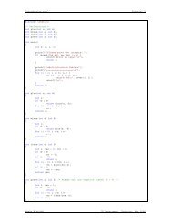
Algorithm 1<br />
Initialize f to harmonic, sm to 1.<br />
Initialize h := argmin h E d LSB (h,f,s,1)<br />
Initialize k using Equation 12<br />
while energy change > ε f do<br />
while energy change > εφ do<br />
{Optimize h for fixed f, k and s.}<br />
h new := argmin h E d LSB (h,f,s,k)<br />
{Perform 1-dimensional search on the line between<br />
h and h new }<br />
t opt = argmin t E d LSB ((1 −t)h +thnew ,f,s(t),k)<br />
h := (1 −t opt )h +t opt h new<br />
Compute k using Equation 12.<br />
end while<br />
{Optimize f for fixed h, k and s}<br />
f := argmin f E d LSB (h,f,s,k)<br />
end while<br />
there is no guarantee that the global minimum is reached<br />
or approximated well. In practice, we observe that the algorithm<br />
converges to the same solution, even for large variations<br />
in the starting point; furthermore, in all our test cases<br />
for which the global minimum is known, the algorithm converges<br />
to this global minimum, as discussed in more detail<br />
in Section 5.<br />
Extension to surfaces. The algorithm directly extends to<br />
mapping genus-zero surfaces with boundary to the plane.<br />
Because quasiconformal distortion is conformally invariant,<br />
it is sufficient to use an arbitrary conformal map of the<br />
surface to the plane, and the composition of this conformal<br />
map with the computed extremal quasiconformal map<br />
is extremal. We use the scale-factor based conformal map<br />
computation to map surfaces to the plane [BGB08, SSP08].<br />
Specifically, for a multiply connected domain of genus zero<br />
we follow these steps:<br />
• One boundary is chosen as external; the remaining boundary<br />
loops are triangulated, reducing the surface to simply<br />
connected.<br />
• The algorithm of [SSP08] is used to compute a logarithmic<br />
scale factor ui for each vertex ui, such that edge<br />
lengths li j = e (ui+u j)/2 define a planar mesh. For the solution<br />
to be unique, we choose the scale factors to be zero<br />
on the outer boundary (i.e., no scale distortion along the<br />
boundary).<br />
• The added triangles are removed to obtain the discrete<br />
conformal image of the original mesh.<br />
We note that the metric used for the conformal map<br />
need not coincide with the Euclidean embedding metric.<br />
This can be used for minimizing different types of errors<br />
in the parametrization (cf. [KMZ10]), as well as “correction”<br />
of a non-bijective parametrization (i.e. nearly flat metric).<br />
If the metric is derived from a different locally bijective<br />
parametrization, there is no need for the flattening conformal<br />
map; however if the parametrization is not locally bijective,<br />
the conformal map is still needed. Figure 18 shows some<br />
examples of this.<br />
c○ 2012 The Author(s)<br />
c○ 2012 The Eurographics Association and Blackwell Publishing Ltd.
O. Weber & A. Myles & D. Zorin / <strong>Computing</strong> <strong>Extremal</strong> <strong>Quasiconformal</strong> <strong>Maps</strong><br />
Discussion. By construction, the quadratic differential computed<br />
by the algorithm is discrete holomorphic and the corresponding<br />
Beltrami coefficient has constant dilatation k. At<br />
the same time, the actual Beltrami coefficient of the map<br />
f¯z/ fz is just an approximation to the “perfect” computed coefficient.<br />
We note that in general, if ˆµ (i.e. the angular part<br />
of µ) is fixed, this determines the parametrization uniquely<br />
with no control for k on each triangle.<br />
While we observe good convergence of the algorithm to<br />
constant k in L 2 norm when the mesh is refined, this does not<br />
guarantee that k < 1 (i.e. there are no fold-overs) on all triangles,<br />
even for a very fine mesh. In practice, we observe that<br />
no triangles are flipped for a sufficiently fine mesh, excluding<br />
few triangles near highly concave parts of the boundary.<br />
In the next section, we present a detailed evaluation of the<br />
behavior of the algorithm: dependency on the starting point,<br />
convergence rates, comparison to analytic cases.<br />
5. Evaluation<br />
Validation. We validate our method in several ways. The<br />
most direct validation is comparison to analytically computed<br />
maps. Unfortunately, the analytic solution is known<br />
explicitly only in few cases. We consider two maps known<br />
analytically: mapping a disk to itself with four boundary<br />
points moved to different locations, and mapping of a ring<br />
to a ring with a different ratio of inner to outer radius. In the<br />
first case, we consider maps moving points at angular locations<br />
±π/4,π ± π/4 on a circle, to ±φ,π ± φ. This map is<br />
given by<br />
fφ(z) = e −iφ <br />
F ze iφ ,e −2iφ<br />
where F(z,w) is the incomplete elliptic integral of the first<br />
kind. For the ring domain with inner and outer radii r0 and<br />
r1, mapped to a ring with inner and outer radii r ′ 0 and r′ 1 , the<br />
extremal map has the polar coordinate form<br />
(r,φ) → (r ′ 0(r/r0) K ,φ)<br />
where K = ln(r ′ 1 /r′ 0 )/ln(r1/r0). In both cases, we observe<br />
an accurate match both for the maps, and extremal dilatation<br />
values.<br />
We can also compute a subclass of Teichmüller maps<br />
semi-analytically, by prescribing a pair of conformal maps,<br />
and a stretch in the intermediate domain. We tested our<br />
method for both analytically and semi-analytically computed<br />
maps (Figure 7).<br />
In analytic cases, the maps are very close to exact ones.<br />
As the piecewise linear maps cannot in general have constant<br />
dilatation, we consider the deviation from the correct<br />
constant k as a measure of error, shown in the figure.<br />
Convergence in the general case. While the optimal dilatation<br />
cannot be computed for general boundary conditions,<br />
one can estimate the rate at which the deviation of dilatation<br />
k from the average value decreases. We observe a similar<br />
behavior for this measure shown in the last two examples<br />
in Figure 7. The number of iterations needed to reach 1%<br />
relative change in energy was typically on the order of 10<br />
c○ 2012 The Author(s)<br />
c○ 2012 The Eurographics Association and Blackwell Publishing Ltd.<br />
k error<br />
0.0004<br />
k error 0.022<br />
k error 0.0037<br />
k error<br />
0.014<br />
k error<br />
0.0026<br />
60<br />
40<br />
20<br />
0<br />
0 0.5 1<br />
100<br />
50<br />
0<br />
0<br />
60<br />
0.5 1<br />
40<br />
20<br />
0<br />
0 0.5 1<br />
80<br />
60<br />
40<br />
20<br />
0<br />
0<br />
80<br />
60<br />
40<br />
20<br />
0.5 1<br />
0<br />
0 0.5 1<br />
Figure 7: Top 3 examples: comparison to extremal quasiconformal<br />
maps. A disk with four points moved along the<br />
boundary, a ring with a change in the ratio of inner-to-outer<br />
radius, and an example of a map computed as a composition<br />
(3). This example shows a comparison of the map directly<br />
computed as the composition (left) with the map computed<br />
using our algorithm (middle). For each example, a histogram<br />
of k is shown, with percentages of triangles along the<br />
vertical axis. The last two examples use prescribed boundary<br />
values not corresponding to a known map.<br />
(in some cases, such as the ring domain, as low as 2-3). On<br />
the other hand, more complex and extreme deformations required<br />
more iterations.<br />
As expected, we observe that zeros of the quadratic differential<br />
become visible in the map (e.g., as shown in Figure 9).<br />
Dependence on initialization. As our algorithm minimizes<br />
a nonlinear energy, in principle the result may depend on the<br />
starting point. However, we observe very little dependence,<br />
as demonstrated in Figure 10.
Distribution error<br />
10 0<br />
10 −1<br />
10 −2<br />
10 −2<br />
10 −3<br />
Shape 1<br />
Shape 2<br />
Shape 3<br />
Shape 4<br />
Shape 5<br />
10 −1<br />
Edge length<br />
10 0<br />
O. Weber & A. Myles & D. Zorin / <strong>Computing</strong> <strong>Extremal</strong> <strong>Quasiconformal</strong> <strong>Maps</strong><br />
Beltrami error<br />
10 0<br />
10 −1<br />
10 −2<br />
10 −3<br />
10 −4<br />
10 −5<br />
10 −6<br />
10 −2<br />
10 −7<br />
Shape 1<br />
Shape 2<br />
Shape 3<br />
Shape 4<br />
Shape 5<br />
10 −1<br />
Edge length<br />
Figure 8: Convergence of k as a function of mesh resolution<br />
for examples of Figure 7; for the ring and four-point disk examples,<br />
new meshes were generated for each resolution; for<br />
remaining examples, the meshes were refined by quadrisection.<br />
Figure 9: After 3 iterations of the algorithm, applied to the<br />
initial harmonic map, zeros of the quadratic differential become<br />
visible; in the final map they appear as isolated spots<br />
of nearly zero k.<br />
Alternative methods for computing the map. As the extremal<br />
quasiconformal maps are defined as minima of the<br />
functional maxz k(z), an obvious alternative is to attempt to<br />
compute the map directly, without relying on its description<br />
as the Teichmüller map. The discrete problem can be formulated<br />
as a the problem of minimizing k with per-triangle<br />
nonlinear inequality constraints km(f) < k. Our experiments<br />
show that with most starting points standard interior-point<br />
or active-set methods do not make much progress on the<br />
problem even in relatively simple cases (Figure 11, matlab<br />
optimization with analytic gradients is used). A common approach<br />
to approximation solutions of L∞ optimization problems<br />
is to use Lp norms with increasing p. For low p, and<br />
high p we have observed bad convergence behavior not producing<br />
meaningful maps. Medium-range values of p (p = 5)<br />
converged (although more than an order of magnitude slower<br />
than our method) but the solution was quite far from the extremal<br />
map.<br />
Comparison with other energies. Figure 15 shows how<br />
our maps compare to several common types of maps obtained<br />
by minimizing other types of energies, that can satisfy<br />
Dirichlet boundary conditions: harmonic/LSCM ( [DMA02,<br />
LPRM02]), ARAP ( [LZX ∗ 08]), and MIPS [HG99]. The<br />
10 0<br />
0.6<br />
0.1<br />
harmonic map ARAP noisy initialization<br />
extremal q.c. map results from above initializations<br />
Figure 10: Dependence on initialization. A screw is mapped<br />
to an annulus using three different initializations. Helical<br />
sharp edges are highlighted to show parametrization flow.<br />
Upper row: Harmonic, ARAP and noisy parametrizations<br />
exhibit 924, 268 and 831 fold-overs respectively (shown in<br />
red). Lower two rows: <strong>Extremal</strong> q.c. maps resolve all foldovers.<br />
The algorithm produces consistent results for each<br />
initialization in the first row.<br />
Beltrami 2-norm 5-norm ∞-norm<br />
Figure 11: Comparison of our method with direct optimization<br />
of maximal k, and optimization of (k) p dA for 3 values<br />
of p. The color indicates the value of k.<br />
first two methods could handle the same boundary constraints,<br />
but produced parametrizations far from bijective.<br />
MIPS had to be initialized with simpler boundary constraints,<br />
for which an initial bijective parametrization can<br />
be obtained. Figures 12 and 13 demonstrate challenging<br />
parametrizations with sharp feature alignments. Figure 14<br />
compares our method to ARAP when applied to deform an<br />
image.<br />
We observe that for our method the final result for higher<br />
resolution meshes is largely independent of mesh connectivity(Figure<br />
16). For simple boundary shapes, the map is typically<br />
well-approximated with relatively few triangles (Figure<br />
17).<br />
Combining with other error metrics. While maximal dilatation<br />
are a natural measure of distortion, it does not cap-<br />
c○ 2012 The Author(s)<br />
c○ 2012 The Eurographics Association and Blackwell Publishing Ltd.<br />
0.6<br />
0.4<br />
0.2
0.7<br />
0.4<br />
0.1<br />
O. Weber & A. Myles & D. Zorin / <strong>Computing</strong> <strong>Extremal</strong> <strong>Quasiconformal</strong> <strong>Maps</strong><br />
harmonic ARAP q.c.<br />
ARAP<br />
Figure 12: Parametrization with aligned sharp features and<br />
boundary. We cut the front of the fandisk model to obtain a<br />
disk-like surface and flatten it while aligning the sharp features<br />
and boundary to parametric lines using harmonic map,<br />
ARAP and our extremal q.c. map. The color visualization<br />
and histograms shows values of k between 0.1 to 0.7.<br />
Figure 13: Parametrization aligned to the boundaries of a<br />
large curved multiply connected model using our q.c. extremal<br />
algorithm. The disk-topology of the surface is maintained.<br />
i.e., no cones or cuts are introduced. Top row: a texture<br />
of regular grid is mapped onto the surface. Bottom row:<br />
a quadrangular mesh (left) is obtained by sampling the parametric<br />
domain (right). In contrast to Figure 18, here we use<br />
the original surface metric.<br />
ture many common types of requirements needed in applications.<br />
For example, the parametrization may need to be close<br />
to isometric, and dilatation does not take area distortion into<br />
account. In other cases, we may want the parametric lines<br />
to be aligned with features etc. One can use extremal quasiconformal<br />
maps in composition with a metric defined using<br />
a different parametrization type as explained in Section 4.2.<br />
Figure 18 shows several examples of this type.<br />
Figure 19 demonstrates the behavior of our algorithm<br />
when pushed to the limit. A multiply connected ball shaped<br />
surface with twelve pentagonal holes is mapped to a disk<br />
without introducing any cuts. One of the holes is mapped<br />
to the boundary of the disk while all the others are mapped<br />
to fixed circles inside the disk. With such extreme boundary<br />
conditions, large amount of conformal distortion is unavoidable.<br />
Nevertheless our algorithm manage to produce a bijective<br />
map without any foldovers. Harmonic map with exact<br />
same boundary conditions is much smoother. However the<br />
c○ 2012 The Author(s)<br />
c○ 2012 The Eurographics Association and Blackwell Publishing Ltd.<br />
source<br />
q.c.<br />
Figure 14: Image deformation. A doughnut is deformed to<br />
have different thickness using ARAP and extremal q.c. map.<br />
Note the foldovers ARAP develops.<br />
Beltrami Harmonic ARAP<br />
Beltrami ARAP MIPS<br />
Figure 15: Comparison of the results for several energies:<br />
an extremal quasiconformal map, harmonic, ARAP, MIPS.<br />
As MIPS energy is infinite at foldovers, it was initialized on a<br />
less challenging configuration with bijective output of ARAP.<br />
conformal distortion is extremely high, leading to more than<br />
800 flipped triangles. ARAP parametrization produce similar<br />
result with more than 600 flipped triangles.<br />
6. Conclusions and future work<br />
From computational point of view, quasiconformal maps,<br />
i.e. maps with globally bounded dilatation, are a natural way<br />
source<br />
irregular<br />
regular<br />
Figure 16: Comparison of maps obtained for regular and<br />
irregular meshes<br />
0.6<br />
0.3<br />
0
O. Weber & A. Myles & D. Zorin / <strong>Computing</strong> <strong>Extremal</strong> <strong>Quasiconformal</strong> <strong>Maps</strong><br />
192 triangles 784 triangles 3136 triangles<br />
Figure 17: A sequence of maps obtained by mapping a<br />
square to a wedge shape; at each resolution, an irregular<br />
mesh is used.<br />
ARAP<br />
q.c.<br />
Figure 18: Combining extremal quasi-conformal<br />
parametrization with other metric. Top, left: ARAP<br />
parametrization; Right: q.c. parametrization in ARAP metric<br />
reduces artifacts near constraints at the cost of increased<br />
distortion elsewhere. Bottom: q.c. parametrization in ARAP<br />
metric is used to move markers to desired positions.<br />
to describe bijective maps, because for practical purposes,<br />
arbitrary high dilatation is as bad as the lack of bijectivity.<br />
This class of maps is almost as broad as all bijective maps,<br />
and considering extremal maps makes it possible to define<br />
a unique quasiconformal solution for problems with fixed<br />
boundaries. As we have demonstrated, although the problem<br />
is nonlinear, extremal maps can be approximated efficiently<br />
extremal q.c.<br />
extremal q.c. harmonic<br />
Figure 19: A ball is mapped to a disk with circular holes.<br />
One of the pentagonal holes on the ball is mapped to the<br />
outer boundary of a disk. A harmonic map results in a map<br />
with more than 800 flipped triangles.<br />
and robustly. At the same time, our approximation does not<br />
guarantee that the resulting approximate map is locally bijective<br />
everywhere.<br />
We view developing a truly discrete concept of extremal<br />
quasiconformal maps as a promising direction. The generalization<br />
is far from trivial, as simply defining the extremal<br />
map as the global minimum of maximal per-triangle dilatation<br />
functional does not retain most attractive properties of<br />
the smooth quasiconformal maps.<br />
Extension to surfaces of arbitrary genus and surfaces<br />
with cones. An important limitation of the described<br />
method is its inability to handle surfaces of arbitrary<br />
genus, and target domains with cones (cf. [SSP08, BGB08,<br />
BZK09]). We briefly outline how these cases can be handled,<br />
leaving a detailed specification of the algorithm and its<br />
practical evaluation as future work.<br />
The overall approach is to use local simply connected<br />
charts to define the map. In fact, a single chart, obtaining by<br />
cutting the surface to a disk is sufficient, but the reasoning is<br />
easier to explain with multiple overlapping charts. Suppose<br />
the surface is covered by such charts.<br />
Recall that the algorithm involves interleaved computation<br />
of a parametrization f (z) and the quadratic differential<br />
φ(z). We can define these locally, using a conformal atlas:<br />
for each chart a conformal map to the plane is defined, assigning<br />
to each point p its coordinate z(p). We assume that<br />
these conformal maps are consistent, i.e. for two overlapping<br />
charts, with coordinates z(p) and z ′ (p), in the overlap area<br />
the composition of conformal coordinates w ◦ z −1 = χ is a<br />
conformal map.<br />
We can now define a parametrization f z and a quadratic<br />
differential φ z for each chart, requiring consistency. The consistency<br />
for the maps f z can be imposed in the usual way, as<br />
it is done in, e.g., [SSP08]: the maps f z and f w coincide,<br />
up to a rigid translation and rotation by an angle kπ/2, i.e.<br />
f w = e ikπ/2 f z . For quadratic differentials the transformation<br />
rule, (see Section 3) is φ w (w)χ 2 z = φ z (z). As the quadratic<br />
differential is related to the metric tensor of f , the rigid transform<br />
between f z and f w values does not affect it.<br />
As a result, we can obtain a similar algorithm for each<br />
chart, with additional constraints imposed on maps and<br />
quadratic differentials between charts.<br />
Acknowledgements<br />
We would like to thank Frederick Gardiner for helpful discussions.<br />
This research was partially supported by NSF<br />
awards IIS-0905502, DMS-0602235 and OSI-1047932.<br />
References<br />
[Ahl53] AHLFORS L.: On quasiconformal mappings. Journal<br />
d’Analyse Mathématique 3, 1 (1953), 1–58. 2<br />
[Ahl66] AHLFORS L.: Lectures on quasiconformal mappings,<br />
vol. 38. Amer. Mathematical Society, 1966. 2<br />
[AS06] A. SHEFFER E. PRAUN K. R.: Mesh parameterization<br />
methods and their applications. Foundations and Trends in Computer<br />
Graphics and Vision 2, 2 (2006). 1<br />
c○ 2012 The Author(s)<br />
c○ 2012 The Eurographics Association and Blackwell Publishing Ltd.
O. Weber & A. Myles & D. Zorin / <strong>Computing</strong> <strong>Extremal</strong> <strong>Quasiconformal</strong> <strong>Maps</strong><br />
[Bal81] BALL J.: Global invertibility of Sobolev functions and<br />
the interpenetration of matter. Proc. Roy. Soc. Edinburgh Sect. A<br />
88, 3-4 (1981), 315–328. 2<br />
[BGB08] BEN-CHEN M., GOTSMAN C., BUNIN G.: Conformal<br />
flattening by curvature prescription and metric scaling. Computer<br />
Graphics Forum 27, 2 (2008), 449–458. 2, 6, 10<br />
[BZK09] BOMMES D., ZIMMER H., KOBBELT L.: Mixedinteger<br />
quadrangulation. ACM Trans. Graph. 28, 3 (2009), 77.<br />
2, 10<br />
[CLR04] CLARENZ U., LITKE N., RUMPF M.: Axioms and variational<br />
problems in surface parameterization. Computer Aided<br />
Geometric Design 21, 8 (2004), 727–749. 2<br />
[Dar93] DARIPA P.: A fast algorithm to solve the Beltrami equation<br />
with applications to quasiconformal mappings. Journal of<br />
Computational Physics 106, 2 (1993), 355–365. 2<br />
[DMA02] DESBRUN M., MEYER M., ALLIEZ P.: Meshes and<br />
parameterization: Intrinsic parameterizations of surface meshes.<br />
Computer Graphics Forum 21, 3 (2002), 209. 2, 8<br />
[ESG01] ECKSTEIN I., SURAZHSKY V., GOTSMAN C.: Texture<br />
mapping with hard constraints. In Computer Graphics Forum<br />
(2001), vol. 20, Wiley Online Library, pp. 95–104. 2<br />
[FH05] FLOATER M., HORMANN K.: Surface parameterization:<br />
a tutorial and survey. Advances In Multiresolution For Geometric<br />
Modelling (2005). 1<br />
[Flo97] FLOATER M.: Parametrization and smooth approximation<br />
of surface triangulations. Computer Aided Geometric Design<br />
14, 3 (1997), 231–250. 2<br />
[Gar] GARDINER. F. P.: Personal communication. 4<br />
[GL00] GARDINER F., LAKIC N.: <strong>Quasiconformal</strong> Teichmüller<br />
theory, vol. 76 of Mathematical Surveys and Monographs. American<br />
Mathematical Society, 2000. 2<br />
[Grö30] GRÖTZSCH H.: Ueber die Verzerrung bei nichtkonformen<br />
schlichten Abbildungen mehrfach zusammenhängender<br />
Bereiche. Leipz. Ber. 82 (1930), 69–80. 2<br />
[GY03] GU X., YAU S.-T.: Global conformal surface parameterization.<br />
In Symposium on Geometry Processing (Aire-la-<br />
Ville, Switzerland, 2003), SGP ’03, Eurographics Association,<br />
pp. 127–137. 2<br />
[HG99] HORMANN K., GREINER G.: MIPS: An efficient global<br />
parameterization method. Curve and Surface Design: Saint-Malo<br />
2000 (1999), 153–162. 2, 8<br />
[JZDG09] JIN M., ZENG W., DING N., GU X.: <strong>Computing</strong><br />
Fenchel-Nielsen coordinates in Teichmuller shape space. In<br />
Shape Modeling International (2009), IEEE, pp. 193–200. 2<br />
[JZLG09] JIN M., ZENG W., LUO F., GU X.: <strong>Computing</strong> Tëichmuller<br />
shape space. Visualization and Computer Graphics 15, 3<br />
(2009), 504–517. 2<br />
[KGG05] KARNI Z., GOTSMAN C., GORTLER S.: Freeboundary<br />
linear parameterization of 3d meshes in the presence<br />
of constraints. In Shape Modeling and Applications, 2005 International<br />
Conference (2005), IEEE, pp. 266–275. 2<br />
[KMZ10] KOVACS D., MYLES A., ZORIN D.: Anisotropic quadrangulation.<br />
Symposium on Solid and Physical Modeling (2010),<br />
137–146. 6<br />
[KNP07] KÄLBERER F., NIESER M., POLTHIER K.: Quad-<br />
Cover: surface parameterization using branched coverings. Computer<br />
Graphics Forum 26, 3 (2007), 375–384. 2<br />
[KSG03] KRAEVOY V., SHEFFER A., GOTSMAN C.: Matchmaker:<br />
constructing constrained texture maps. In ACM Trans.<br />
Graph. (2003), vol. 22, ACM, pp. 326–333. 2<br />
[KSS06] KHAREVYCH L., SPRINGBORN B., SCHRÖDER P.:<br />
Discrete conformal mappings via circle patterns. ACM Trans.<br />
Graph. 25 (April 2006), 412–438. 2<br />
c○ 2012 The Author(s)<br />
c○ 2012 The Eurographics Association and Blackwell Publishing Ltd.<br />
[Lév01] LÉVY B.: Constrained texture mapping for polygonal<br />
meshes. In Proc. Computer graphics and interactive techniques<br />
(2001), ACM, pp. 417–424. 2<br />
[LKF12] LIPMAN Y., KIM V., FUNKHOUSER T.: Simple formulas<br />
for quasiconformal plane deformations. ACM Trans. Graph.<br />
(2012). to appear. 2<br />
[LPRM02] LÉVY B., PETITJEAN S., RAY N., MAILLOT J.:<br />
Least squares conformal maps for automatic texture atlas generation.<br />
ACM Trans. Graph. 21, 3 (2002), 362–371. 2, 8<br />
[LWT ∗ 10] LUI L., WONG T., THOMPSON P., CHAN T., GU X.,<br />
YAU S.: Shape-based diffeomorphic registration on hippocampal<br />
surfaces using Beltrami holomorphic flow. Med. Image Comput.<br />
and Comp.-Assisted Intervention (2010), 323–330. 2<br />
[LZX ∗ 08] LIU L., ZHANG L., XU Y., GOTSMAN C., GORTLER<br />
S. J.: A local/global approach to mesh parameterization. Computer<br />
Graphics Forum 27, 5 (July 2008), 1495–1504. 2, 8<br />
[Rei02] REICH E.: <strong>Extremal</strong> quasiconformal mappings of the<br />
disk. Handbook of Complex Analysis 1 (2002), 75–136. 4<br />
[RLL ∗ 06] RAY N., LI W., LÉVY B., SHEFFER A., ALLIEZ P.:<br />
Periodic global parameterization. ACM Trans. Graph. 25, 4<br />
(2006), 1460–1485. 2<br />
[SdS01] SHEFFER A., DE STURLER E.: Parameterization of<br />
faceted surfaces for meshing using angle-based flattening. Engineering<br />
with Computers 17, 3 (2001), 326–337. 2<br />
[SM04] SHARON E., MUMFORD D.: 2d-shape analysis using<br />
conformal mapping. In Computer Vision and Pattern Recognition<br />
(2004), vol. 2, IEEE, pp. II–350. 2<br />
[SSGH01] SANDER P., SNYDER J., GORTLER S., HOPPE H.:<br />
Texture mapping progressive meshes. In Proc. Computer graphics<br />
and interactive techniques (2001), ACM, pp. 409–416. 2<br />
[SSP08] SPRINGBORN B., SCHRÖDER P., PINKALL U.: Conformal<br />
equivalence of triangle meshes. ACM Trans. Graph. 27<br />
(August 2008), 77:1–77:11. 2, 5, 6, 10<br />
[Tei40] TEICHMÜLLER O.: <strong>Extremal</strong>e quasikonforme Abbildungen<br />
und quadratische Differentiale. Preuss. Akad. Math.-Nat., 22<br />
(1940). 2<br />
[Tei43] TEICHMÜLLER O.: Bestimmung der extremalen<br />
quasikonformen Abbildungen bei geschlossenen orientierten<br />
Riemannschen Flächen. Preuss. Akad. Math.-Nat. 4 (1943). 2<br />
[Tut63] TUTTE W.: How to draw a graph. Proc. London Math.<br />
Soc 13, 3 (1963), 743–768. 2<br />
[WDC ∗ 09] WANG Y., DAI W., CHOU Y., GU X., CHAN T.,<br />
TOGA A., THOMPSON P.: Studying brain morphometry using<br />
conformal equivalence class. In Computer Vision, 12th International<br />
Conference on (2009), IEEE, pp. 2365–2372. 2<br />
[ZLYG09] ZENG W., LUO F., YAU S., GU X.: Surface quasiconformal<br />
mapping by solving Beltrami equations. Mathematics<br />
of Surfaces XIII (2009), 391–408. 2<br />
[ZRS05] ZAYER R., ROSSL C., SEIDEL H.: Discrete tensorial<br />
quasi-harmonic maps. Proc. Shape Modeling and Applications<br />
(2005), 276–285. 2