MA651 Topology. Lecture 2. Elements of Set Theory 2.
MA651 Topology. Lecture 2. Elements of Set Theory 2.
MA651 Topology. Lecture 2. Elements of Set Theory 2.

You also want an ePaper? Increase the reach of your titles
YUMPU automatically turns print PDFs into web optimized ePapers that Google loves.
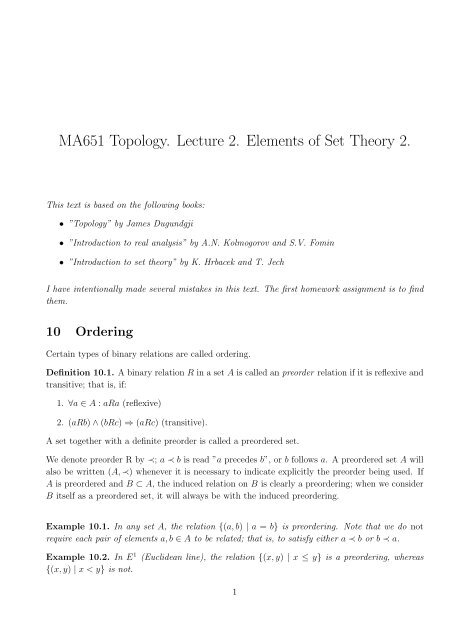
<strong>MA651</strong> <strong>Topology</strong>. <strong>Lecture</strong> <strong>2.</strong> <strong>Elements</strong> <strong>of</strong> <strong>Set</strong> <strong>Theory</strong> <strong>2.</strong><br />
This text is based on the following books:<br />
• ”<strong>Topology</strong>” by James Dugundgji<br />
• ”Introduction to real analysis” by A.N. Kolmogorov and S.V. Fomin<br />
• ”Introduction to set theory” by K. Hrbacek and T. Jech<br />
I have intentionally made several mistakes in this text. The first homework assignment is to find<br />
them.<br />
10 Ordering<br />
Certain types <strong>of</strong> binary relations are called ordering.<br />
Definition 10.1. A binary relation R in a set A is called an preorder relation if it is reflexive and<br />
transitive; that is, if:<br />
1. ∀a ∈ A : aRa (reflexive)<br />
<strong>2.</strong> (aRb) ∧ (bRc) ⇒ (aRc) (transitive).<br />
A set together with a definite preorder is called a preordered set.<br />
We denote preorder R by ≺; a ≺ b is read ”a precedes b”, or b follows a. A preordered set A will<br />
also be written (A, ≺) whenever it is necessary to indicate explicitly the preorder being used. If<br />
A is preordered and B ⊂ A, the induced relation on B is clearly a preordering; when we consider<br />
B itself as a preordered set, it will always be with the induced preordering.<br />
Example 10.1. In any set A, the relation {(a, b) | a = b} is preordering. Note that we do not<br />
require each pair <strong>of</strong> elements a, b ∈ A to be related; that is, to satisfy either a ≺ b or b ≺ a.<br />
Example 10.<strong>2.</strong> In E 1 (Euclidean line), the relation {(x, y) | x ≤ y} is a preordering, whereas<br />
{(x, y) | x < y} is not.<br />
1
Example 10.3. Let C be the set <strong>of</strong> complex numbers, and define z1 ≺ z2 if and only if |z1| ≤ |z2|.<br />
This is a preordering on C. Observe that we do not require that (a ≺ b) ∧ (b ≺ a) imply a = b.<br />
Example 10.4. In P(X), the relation A ≺ B, defined by A ≺ B if and only if A ⊂ B, is a<br />
preordering. More generally, any family <strong>of</strong> sets preordered in this matter is said to be preordered<br />
by inclusion.<br />
There is a standard terminology pertaining to preordered sets:<br />
Definition 10.<strong>2.</strong> Let (A, ≺) be preordered:<br />
1. m ∈ A is called a maximal element in A if ∀a : m ≺ a ⇒ a ≺ m; that is, if neither no a ∈ A<br />
follows m or each a that follows m also precedes m.<br />
<strong>2.</strong> a0 ∈ A is called as upper bound for a subset B ⊂ A if ∀b ∈ B : b ≺ a0.<br />
3. B ⊂ A is called a chain in A if each two elements in B are related<br />
Example 10.5. In Example (10.1), each element is maximal. No subset <strong>of</strong> A containing at least<br />
two elements has an upper bound. Thus a maximal element in A need not be an upper bound for<br />
A.<br />
Example 10.6. In Example (10.2), there is no maximal element. Every bounded set has many<br />
upper bounds.<br />
Example 10.7. In Example (10.3), a0 = 1 is an upper bound for B = {z | |z| ≤ 1} ⊂ C, but<br />
is not maximal in C. Note also that although a0 is an upper bound for B, it is possible for some<br />
b ∈ B also to satisfy a0 ≺ b. In the set B (with induced preorder!) each z with |z| = 1 is both<br />
maximal and upper bound for B.<br />
Placing additional requirements on preorderings gives other types <strong>of</strong> ordering relations.<br />
Definition 10.3. A preordering in A with the additional property<br />
(a ≺ b) ∧ (b ≺ a) ⇒ (a = b) (antisymmetry)<br />
is called a partial ordering. A set together with a definite partial ordering is called a partially<br />
ordered set. A partially ordered set that is also a chain is called a totally ordered set.<br />
It is evident that partial (total) orders induce partial (total) orders on subsets.<br />
Example 10.8. Ordering by inclusion in P(X), or any family <strong>of</strong> sets, is always a partial ordering<br />
(but, clearly, need not be a total order).<br />
2
Example 10.9. Let (A, ≺) be a preordered set, and define a relation S in A by aSb ⇔ (a ≺<br />
b) ∧ (b ≺ a). It is easy to verify that S is an equivalence relation and that A/S is partially ordered<br />
by Sa ≺ Sb ⇔ a ≺ b.<br />
Note that in a partially ordered A, the statement ”m is maximal” is equivalent to ”each a ∈ A is<br />
either not related to m or satisfies only a ≺ m”, and also that if a0 is an upper bound for B ⊂ A,<br />
then there can be no b ∈ B − {a0} with a0 ≺ b.<br />
Total ordering <strong>of</strong> the type in the following definition is very important, as we shall see.<br />
Definition 10.4. A partially ordered set W is called well-ordered (or as ordinal) if each nonempty<br />
subset B ⊂ W has a first element; that is, for each B = Ø, there exists a b0 ∈ B satisfying b0 ≺ b<br />
for each b ∈ B.<br />
Every well-ordered set W is in fact totally ordered, since each subset {a, b} ⊂ W has a first<br />
element; furthermore, the induced order on a subset <strong>of</strong> a well-ordered set is a well-order on that<br />
subset.<br />
Example 10.10. Ø is a well-ordered set. In any set {a} containing exactly one element, a ≺ a<br />
is well-ordering. The partial ordering by inclusion in P(X) is not a well-ordering if X has more<br />
than one element.<br />
Example 10.11. The nonnegative integers are well-ordered: this is one <strong>of</strong> the ways to state the<br />
principle <strong>of</strong> mathematical induction. This well-ordered set is denoted by ω; that is, ω = (N, ≤).<br />
Let W be well-ordered, and q ∈ W ; in W {q} define an order that coincides with the given one<br />
on W , satisfies q ≺ q, and ∀w : (w ∈ W ) ⇒ w ≺ q. Then W {q} is well-ordered, since for each<br />
nonempty E ⊂ W {q}, either E = {q} or E W = Ø, and in the latter case, the first element<br />
in E W is the first in E ⊂ W {q}. We say W {q} is formed from W by adjoining q as last<br />
element.<br />
Each element w <strong>of</strong> a well-ordered set that has a successor in the set, has an immediate successor;<br />
that is, we can find as s = w satisfying w ≺ s and such that no c = s, w satisfies w = c = s; we<br />
need only choose s = first element in the nonempty set {x ∈ W | (w ≺ x) ∧ (w = x)}. However,<br />
an element w need not have an immediate predecessor; for each b ≺ w there may always be some<br />
c = b, w with b ≺ c ≺ w. In fact, adjoining to w a last element q, we note that q has no immediate<br />
predecessor.<br />
11 Zorn’s Lemma; Zermelo’s Theorem<br />
This fundamental theorem is presented without prove:<br />
3
Theorem 11.1. The following three statements are equivalent:<br />
1. The axiom <strong>of</strong> choice: Given any nonempty family {Aα | α ∈ A } <strong>of</strong> nonempty pairwise<br />
disjoint sets, there exists a set S consisting <strong>of</strong> exactly one element from each Aα.<br />
<strong>2.</strong> Zorn’s lemma: Let X be preordered set. If each chain in X has an upper bound, then X has<br />
at least one maximal element.<br />
3. Zermelo’s theorem: Every set can be well ordered.<br />
Remarks Though Zermelo’s theorem assures that every set can be well-ordered, no specific<br />
construction for well-ordering any uncountable set (say, the real numbers) is known. Furthermore,<br />
there are sets for which no specific constructions <strong>of</strong> a total order (let alone a well-order) is known,<br />
for example, the set <strong>of</strong> real-valued functions <strong>of</strong> one variable. Note, also, that a well-ordering<br />
guaranteed by Zermelo’s theorem is obviously not unique, and is not stated to have any relation<br />
to any given structure on the set. For example, a well-ordering <strong>of</strong> the reals cannot coincide with<br />
usual ordering.<br />
Applications<br />
1. Zorn’s lemma is a particularly useful version <strong>of</strong> the axiom <strong>of</strong> choice. It is applicable for<br />
existence theorems whenever the underlying set is partially ordered and the required object<br />
is characterized by maximality. As a simple example <strong>of</strong> its use, we prove the existence <strong>of</strong> a<br />
Hamel basis B for the real numbers.<br />
A subset B = {bα ∈ A } ⊂ E 1 is a Hamel basis if<br />
(a) each real x can be written as a finite sum<br />
with rational rαi<br />
x =<br />
n<br />
1<br />
rαi bαi<br />
(b) the set {bα | α ∈ A } is rationally independent, that is,<br />
n<br />
rαibαi = 0 ⇔ rαi = 0 for each i = 1, · · · , n.<br />
1<br />
The rational independence assures that each x can be written as required by the first condition<br />
(1a) in exactly one way.<br />
To prove existence <strong>of</strong> B, let A be the family <strong>of</strong> all rationally independent sets <strong>of</strong> reals.<br />
A = Ø, since, say, {1} ∈ A . Partially order A by inclusion. Then any chain {Aβ | β ∈ B}<br />
4
has an upper bound, <br />
Aβ, since any finite collection <strong>of</strong> elements in <br />
Aβ lies in some<br />
β<br />
one Aβ and so is rationally independent. Thus there is a maximal B ∈ A ; B is a Hamel<br />
basis, since for each x, B {x} is not rationally independent and therefore there is a relation<br />
zx + rα1xα1 + · · · + rαnxαn = 0, which necessarily involves x and has r = 0 because B is<br />
rationally independent, so that<br />
as required.<br />
x = −<br />
n<br />
1<br />
rαi<br />
r bαi<br />
Hamel bases arise in several connections: If b1 ∈ B, then the set <strong>of</strong> reals generated by B − b1<br />
is not a Lebesgue measurable set. Similarly, the functional equation f(x + y) = f(x) + f(y),<br />
which has f(x) = cx as its only continuous solutions, has others also, none <strong>of</strong> which is a<br />
Lebesgue measurable function.<br />
<strong>2.</strong> In a commutative ring R with unit, every ideal I = R is contained in a maximal ideal<br />
(Krull’s theorem). The pro<strong>of</strong> is immediate by verifying that the set <strong>of</strong> all ideals containing<br />
I , and not containing 1, satisfies the requirement <strong>of</strong> Zorn’s lemma.<br />
Since in R every maximal ideal is a prime ideal, this has an immediate consequence the<br />
following result: Let X be an infinite set. Then there exists a µ : P(X) → {0} ∪ {1}<br />
such that µ(F ) = 0 if F is finite, µ(X) = 1, and µ(A B) = µ(A) + µ(B) whenever A,<br />
B, are disjoint. (In the Boolean ring, P(X) (see Remark, <strong>Lecture</strong> notes 1 p. 6), let F be<br />
a maximal ideal containing the ideal <strong>of</strong> all finite subsets, and set µ(A) = 0 if A ∈ F and<br />
µ(A) = 1 otherwise.)<br />
12 Ordinals<br />
Since every set can be well-ordered, we study ordinals in greater details.<br />
Definition 1<strong>2.</strong>1. Let W be a well-ordered set.<br />
1. S ⊂ W is an ideal in W if ∀x : (x ∈ S) ∧ (y ≺ x) ⇒ y ∈ S.<br />
<strong>2.</strong> For each a ∈ W , the set W (a) = {x ∈ W | (x ≺ a) ∧ (x = a)} is the initial interval<br />
determined by a.<br />
Clearly, W and Ø are ideals in W ; Ø is also an initial interval, but W is not. For the properties<br />
and interrelations <strong>of</strong> these concepts we have<br />
5<br />
β
Proposition 1<strong>2.</strong>1.<br />
1. Every intersection, and every union, <strong>of</strong> ideals in W is itself an ideal in W .<br />
<strong>2.</strong> Let I(W ) be the set <strong>of</strong> all ideals in W and J(W ) the set <strong>of</strong> all initial intervals in W . Then<br />
J(W ) = I(W ) − {W } : the ideals = W are the initial intervals.<br />
Pro<strong>of</strong>. 1. (x ∈ <br />
Sα) ∧ (y ≺ x) ⇒ ∀α : (x ∈ Sα ∧ (y ≺ x) ⇒ ∀α : y ∈ Sα ⇒ y ∈ <br />
Sα, and<br />
α<br />
similarly the union.<br />
<strong>2.</strong> Each interval is obviously an ideal. Conversely, let S = W be an ideal; then W − S = Ø, it<br />
has a first element a. We prove S = W (a).<br />
i x ∈ W (a) ⇒ x ∈ S, since a is the first element <strong>of</strong> W not in S.<br />
ii x ∈ W (a) ⇔ a ≺ x ⇒ x ∈ S, since otherwise, because S is an ideal, we would have<br />
a ∈ S.<br />
Definition 1<strong>2.</strong><strong>2.</strong> A map f <strong>of</strong> a well-ordered set (W, ≺) into a well-ordered (X, ≺ ′ ) is called a<br />
monomorphism if it is an order-preserving injection [that is, a ≺ b ⇒ f(a) ≺ f(b)]; f is an<br />
isomorphism if it is a bijective monomorphism.<br />
Clearly, the composition <strong>of</strong> two monomorphisms is also a monomorphism. It is easy to see that if<br />
f : W → A is an order-preserving bijection and W is well-ordered, then the order in A is also a<br />
well-ordering and f is an isomorphism.<br />
Theorem 1<strong>2.</strong>1.<br />
1. The set I(W ) <strong>of</strong> all ideals <strong>of</strong> a well-ordered set is well-ordered by inclusion.<br />
<strong>2.</strong> The map a → W (a) is an isomorphism <strong>of</strong> W onto the set J(W ) <strong>of</strong> its initial intervals [Ø<br />
included in J(W ) ⊂ I(W )].<br />
Pro<strong>of</strong>. (2) Clearly, a ≺ b ⇒ W (a) ⊂ W (b) and a = b ⇒ W (a) = W (b); thus a → W (a) is<br />
bijective and [using order by inclusion in J(W )] order-preserving. It follows at once that<br />
J(W ) is well-ordered by inclusion and that a → W (a) is an isomorphism.<br />
(1) Since<br />
I(W ) = J(W ) {W }<br />
and since the ordering by inclusion in I(W ) is determined by adjoining {W } as last element,<br />
I(W ) is also well-ordered.<br />
6<br />
α
One consequence is the extremely useful<br />
Theorem 1<strong>2.</strong><strong>2.</strong> Let W be well-ordered, and Σ ⊂ I(W ) any family with the following properties:<br />
(a) Any union <strong>of</strong> members <strong>of</strong> Σ belongs to Σ.<br />
(b) If W (a) ∈ Σ, then also W (a) {a} ∈ Σ.<br />
Then Σ = I(W ) and, in particular, W ∈ Σ.<br />
Pro<strong>of</strong>. Assume Σ = I(W ); by the previous theorem there is a smallest ideal S ∈ Σ. Either S has<br />
a last element, or it does not.<br />
(i) If S has a last element, b, then S = W (b) {b}; because W (b) ⊂ S, we would then have<br />
W (b) ∈ Σ and, by using (b), that S ∈ Σ, which contradicts the definition <strong>of</strong> S.<br />
(ii) If S does not have a last element, then S = {W (a) | W (a) ⊂ S}; as before, each W (a) ∈ Σ,<br />
so by using (a), we conclude that S ∈ Σ, again contradicting the definition <strong>of</strong> S.<br />
Thus, the assumption Σ = I(W ) is false, and the theorem has been proved.<br />
13 The concept <strong>of</strong> ordinal numbers<br />
In the class <strong>of</strong> all ordinals, define W = X if W is isomorphic to X. This is evidently an equivalence<br />
relation, so it divides the class <strong>of</strong> all ordinals into mutually exclusive subclasses. We wish to attach<br />
to each ordinal an object, called its ordinal number, so that two ordinals have the same ordinal<br />
number if and only if they are isomorphic. Following Frege, we could define the ordinal number<br />
<strong>of</strong> an ordinal to be the equivalence class <strong>of</strong> the ordinal. Though this definition is adequate for<br />
most mathematical purposes, it has the disadvantage that ordinal numbers are not sets: Without<br />
separate axiomatic for them, we could not, for example, legitimately consider any collection <strong>of</strong><br />
ordinal numbers. To develop this axiomatics it is enough to show that there exist a uniquely<br />
defined well-ordered class L such that each well-ordered set is isomorphic to some initial interval<br />
<strong>of</strong> L . The desired objective is attained by calling the members <strong>of</strong> L ordinals numbers and<br />
assigning to each ordinal W the α ∈ L for which W = L (α).<br />
The basic idea is to use the sets postulated by the axiom <strong>of</strong> infinity. Then each α ∈ L will be<br />
a set whose elements are all the sets in L that precede it; in other words, each α ∈ L will be<br />
simply the initial interval L (α) in L . To illustrate the mechanics, we write down the first few<br />
members <strong>of</strong> L :<br />
Ø; {Ø}; {Ø, {Ø}}; {Ø, {Ø}, {Ø, {Ø}}}.<br />
The ordinal number <strong>of</strong> {1, 2, 3}, in its natural order, is then {Ø, {Ø}, {Ø, {Ø}}}<br />
If the set is infinite, the ordinal number is said to be transfinite.<br />
7
14 Comparison <strong>of</strong> ordinal numbers<br />
If n1 and n2 are two finite ordinal numbers, then they either coincide or else one is large than the<br />
other. As we now show, the same is true <strong>of</strong> transfinite ordinal numbers. Given any two ordinal<br />
numbers α and β corresponding to the well-ordered sets W and V respectively. Then we can say<br />
that<br />
• α = β if W and V are isomorphic;<br />
• α < β if W is isomorphic to some initial interval <strong>of</strong> V ;<br />
• α > β if V is isomorphic to some initial interval od W<br />
(note that this definition makes sense for finite α and β).<br />
Lemma 14.1. Let f be an isomorphism <strong>of</strong> a well-ordered set A onto some subset B ⊂ A. Then<br />
f(a) ≥ a for all a ∈ A.<br />
Pro<strong>of</strong>. If there are elements a ∈ A such that f(a) ≥ a, then there is a least such element since<br />
A is well-ordered set. Let a0 be this element and let b0 = f(a0). Then b0 < a0, and hence<br />
f(b0) < f(a0) = b0 since f is an isomorphism. But then a0 is not the smallest element such that<br />
f(a) < a. Contradiction.<br />
It follows from this lemma that a well-ordered set A cannot be isomorphic to any <strong>of</strong> its initial<br />
intervals, since if A were isomorphic to the initial interval determined by a, then clearly f(a) < a.<br />
In other words, the two relations<br />
are incompatible, and so are<br />
Moreover, the two relations<br />
α = β, α < β<br />
α = β, α > β<br />
α < β, α > β<br />
are incompatible, since otherwise we could use the transitivity to deduce α < α, which is impossible<br />
by the lemma. Therefore, if one <strong>of</strong> the three relations<br />
(1) α < β, α = β α > β<br />
holds, the other two are automatically excluded. We must still show that one <strong>of</strong> relations (1)<br />
always holds, thereby providing that any two ordinal numbers are compatible.<br />
Theorem 14.1. Two given ordinal numbers α and β satisfy one and only one <strong>of</strong> the relations<br />
α < β, α = β, α > β<br />
8
Pro<strong>of</strong>. Let W (α) be the set <strong>of</strong> all ordinal numbers < α. Any two numbers γ and γ ′ in W (α)<br />
are comparable and the corresponding ordering <strong>of</strong> W (α) makes it a well-ordered set with ordinal<br />
number α. In fact, if is a set<br />
A = {. . . , a, . . . , b, . . .}<br />
has ordinal number α, then by definition, the ordinals corresponding to the ordinal numbers less<br />
than α are isomorphic to some initial interval <strong>of</strong> A. Hence the ordinal numbers themselves are in<br />
one-to-one correspondence with the elements <strong>of</strong> A.<br />
Now let α and β be any two ordinal numbers corresponding to well-ordered sets W (α) and W (β)<br />
respectively. Moreover, let C = A B be the intersection <strong>of</strong> the sets A and B, i.e. sets <strong>of</strong> all<br />
ordinals less than both α and β. Then C is well-ordered with ordinal number γ, say. We now<br />
show that γ ≤ α. If C = A then obviously γ = α. On the other hand, if C = A, then C is an<br />
initial interval <strong>of</strong> A and hence γ < α. In fact, let ξ ∈ C, η ∈ A − C. Then ξ and η are compatible,<br />
i.e., either ξ < η or ξ > η. but η < ξα is impossible, since then η ∈ C. Therefore ξ < η and<br />
hence C is an initial interval <strong>of</strong> A, which implies γ < α. Moreover, γ is the first element <strong>of</strong> the<br />
set A − C. Thus γ ≤ α, as asserted, and similarly γ ≤ β. The case γ < α, γ < β is impossible,<br />
since then γ ∈ A − C, γ ∈ B − C. But then γ ∈ C on the one hand and γ ∈ A B = C on the<br />
other hand. It follows that there are only three possibilities<br />
15 Transfinite induction<br />
γ = α, γ = β, α = β<br />
γ = α, γ < β, α < β<br />
γ < α, γ = β, α > β<br />
Mathematical propositions are very <strong>of</strong>ten proved by using the following familiar<br />
Theorem 15.1. Mathematical induction Given a proposition P (n) formulated for every positive<br />
integer n, suppose that<br />
(1) P (1) is true;<br />
(2) The validity <strong>of</strong> P (k) for all k ≤ n implies the validity <strong>of</strong> P (n + 1).<br />
Then P (n) is true for all n = 1, 2, . . .<br />
Pro<strong>of</strong>. Suppose P (n) fails to be true for all n = 1, 2, . . ., and let n1 be smallest integer for which<br />
P (n) is false (the existence <strong>of</strong> n1 follows from the well-ordering <strong>of</strong> the positive integers). Clearly<br />
n1 > 1, so that n1 − 1 is a positive integer. Therefore P (n) is valid for all k ≤ n1 − 1 but not for<br />
n1. Contradiction.<br />
9
Replacing the set <strong>of</strong> all integers by an arbitrary well-ordered set, we get<br />
Theorem 15.<strong>2.</strong> Transfinite induction Given a well ordered set A, let P (a) be a proposition<br />
formulated for every element a ∈ A. Suppose that<br />
(1) P (1) is true for the smallest element <strong>of</strong> A;<br />
(2) The validity <strong>of</strong> P (a) for all a < a ∗ implies the validity <strong>of</strong> P (a ∗ ).<br />
Then P (a) is true for all a ∈ A.<br />
Pro<strong>of</strong>. Suppose P (a) fails to be true for all a ∈ A. Then P (a) is false for all a in some nonempty<br />
subset A ∗ ⊂ A. By the well-ordering, A ∗ has a smallest element a ∗ . Therefore P (a) is valid for<br />
all a < a ∗ but not for a ∗ . Contradiction.<br />
Remark Since any set can be well-ordered by Zermelo’s theorem, transfinite induction can in<br />
principle can be applied to any set M whatsoever. In practice, however, Zorn’s lemma is a more<br />
useful tool, requiring only that M be partially ordered.<br />
16 Cardinality <strong>of</strong> <strong>Set</strong>s<br />
The ordinals are associated with counting: to count, one counts some elements first and thus<br />
tacitly induced a well-ordering. The concept <strong>of</strong> cardinal is related simply to size: we wish to<br />
determine if one <strong>of</strong> two given sets has more members than the other. Counting is not needed for<br />
this purpose: we need only pair <strong>of</strong>f each member <strong>of</strong> one set with a member <strong>of</strong> the other and see if<br />
any elements are left over. ”Same size” is thus formalized in<br />
Definition 16.1. Two sets, X and Y , are equipotent (or have the same cardinal) if a bijective<br />
map <strong>of</strong> X onto Y exists. We denote ”X equipotent to Y ” by ”card X = card Y ”.<br />
The next simple theorem shows that equipotence is an equivalence relation in the class <strong>of</strong> all sets,<br />
so it decomposes this class into mutually exclusive subclasses, called equipotence classes.<br />
Theorem 16.1. Let A, B, and C be sets, then<br />
1. A is equipotent to A<br />
<strong>2.</strong> If A is equipotent to B, then B is equipotent to A<br />
3. If A is equipotent to B and B is equipotent to C, then A is equipotent to C<br />
Pro<strong>of</strong>.<br />
10
1. The identity function (IdA) which returns the same value that was used as its argument<br />
(f(x) = x) for all elements <strong>of</strong> A is a bijective map <strong>of</strong> A onto A.<br />
<strong>2.</strong> If f is a bijective map <strong>of</strong> A onto B then f −1 is a bijective map <strong>of</strong> B onto A.<br />
3. If f is a bijective map <strong>of</strong> A onto B and g is a bijective map <strong>of</strong> B onto C, then f ◦ g is a<br />
bijective map <strong>of</strong> A onto C<br />
Example 16.1. Let X = {2n | n ∈ N} ⊂ N. Then card X = card N, since n → 2n is a bijective<br />
<strong>of</strong> N onto X. Note that a set may be equipotent with a proper subset.<br />
Example 16.<strong>2.</strong> Any open interval ]a, b[⊂ E 1 is equipotent to J =]−1, +1[, since x → b−a<br />
2<br />
is a bijection J →]a, b[. Furthermore, J is equipotent with E 1 , as x → x<br />
1+|x|<br />
x+ b+a<br />
2<br />
shows. Thus, by<br />
transitivity, card ]a, b[ = card E 1 : each open interval in E 1 has ”just as many points” as E 1 itself.<br />
Definition 16.<strong>2.</strong> For two sets X, Y , the cardinality <strong>of</strong> X is less than or equal to the cardinality<br />
<strong>of</strong> Y , and we write card X ≤ card Y if an injection X → Y exists.<br />
Note that we use ”≤” rather than ”smaller”: The existence <strong>of</strong> an injection X → Y does not<br />
exclude the possibility that there is also a bijection X → Y .<br />
The next evident proposition and the following theorem show that the property card X ≤ card<br />
Y behaves like an ordering on the ”equivalence classes” under equipotence.<br />
Proposition 16.1. Let X, Y, and Z be sets, then<br />
1. If card X ≤ card Y and card X = card Z, then card Z ≤ card Y<br />
<strong>2.</strong> If card X ≤ card Y and card Y = card Z, then card X ≤ card Z<br />
3. card X ≤ card X<br />
4. If card X ≤ card Y , and card Y ≤ Z, then card X ≤ card Z<br />
We see that ≤ is reflexive and transitive. It remains to establish antisymmetry.<br />
Theorem 16.<strong>2.</strong> Cantor-Bernstein<br />
If card X ≤ card Y and card Y ≤ card X, then card X = card Y .<br />
11
Pro<strong>of</strong>. If card X ≤ card Y , then there is an injection f that maps X into Y ; if card Y ≤ card<br />
X, then there is an injection g that maps Y into X. To show that card X = card Y we have to<br />
exhibit a one-to-one function which maps X onto Y .<br />
Let us apply first f and then g; the function g ◦ f maps X into X and is an injection. Clearly,<br />
g(f(X)) ⊂ g(Y ) ⊂ X; moreover, since f and g are one-to-one, we have card X = card g(f(X)).<br />
Then to prove this theorem we should prove the following equivalent proposition (which is also<br />
sometimes called ”Cantor-Bernstein theorem”): Given any two sets A and B, suppose A contains<br />
a subset A1 equipotent to B, while B contains a subset B1 equivalent to A. Then A and B are<br />
equipotent.”<br />
By hypothesis there is one-to-one function f mapping A into B1 and one-to-one function g mapping<br />
B into A1:<br />
f(A) = B1 ⊂ B, g(B) = A1 ⊂ A<br />
therefore<br />
is a subset <strong>of</strong> A1 equipotent to A. Similarly<br />
A2 = gf(A) = g(f(A)) = g(B1)<br />
B2 = fg(B) = f(g(B)) = f(A1)<br />
is a subset <strong>of</strong> B1 equipotent to B. Let A3 be the subset <strong>of</strong> A into which the mapping gf carries<br />
the set A1, and let A4 be the subset <strong>of</strong> A into which gf carries A<strong>2.</strong> More generally, let Ak+2 be<br />
the set into which Ak (k = 1, 2, ...) is carried by gf. Then clearly<br />
<strong>Set</strong>ting<br />
A ⊃ A1 ⊃ A2 ⊃ · · · ⊃ Ak ⊃ Ak+1 · · ·<br />
D =<br />
we can represent A as the following union <strong>of</strong> pairwise disjoint sets:<br />
∞<br />
k=1<br />
A1 = (A − A1) (A1 − A2) (A2 − A3) · · · (Ak − Ak+1) · · · D<br />
Clearly, A and A1 can be represented as<br />
Ak<br />
A = D M N<br />
A1 = D M N1<br />
12
where<br />
M = (A1 − A2) (A3 − A4) · · ·<br />
N = (A − A1) (A2 − A3) · · ·<br />
N1 = (A2 − A3) (A4 − A5) · · ·<br />
But A−A1 is equipotent to A2 −A3 (the former is carried into the later by the one-to-one function<br />
gf), A2 − A3 is equipotent to A4 − A5. and so on. Therefore N is equipotent to N1 and therefore<br />
the one-to-one correspondence can be set up between the sets A and A1. But A1 is equipotent to<br />
B, by hypothesis. Therefore A is equivalent to B.<br />
Remark. Here we can even ”afford the unnecessary luxury” <strong>of</strong> explicitly writing down a one-toone<br />
function carrying A into B, i.e.,<br />
<br />
−1 g if a ∈ D<br />
ϕ(a) =<br />
M<br />
f(a) if a ∈ D N<br />
17 Finite, Countable and Uncountable <strong>Set</strong>s<br />
In this section we list some basic facts concerning finite, countable and uncountable sets. We do<br />
not prove them, but students are encouraged to read the first chapter <strong>of</strong> the James Munkres’s<br />
book, where some pro<strong>of</strong>s are given. For the comprehensive theory <strong>of</strong> sets we refer to ”Introduction<br />
to set theory” by K. Hrbacek and T. Jech.<br />
Definition 17.1. A set S is finite if it is equipotent to some natural number n ∈ N. We then<br />
define card S = n and say that S has n elements. A set is infinite if it not finite.<br />
Finite sets<br />
Proposition 17.1. If n ∈ N , then there is no one-to-one mapping <strong>of</strong> n onto a proper subset<br />
X n<br />
Corollary 17.1. • If n = m, then there is no mapping <strong>of</strong> n onto m.<br />
• If card S = n and card S = m, then n = m.<br />
• N is infinite.<br />
Proposition 17.<strong>2.</strong> If X is a finite set and Y ⊂ X, then Y is finite. moreover card Y ≤ card X.<br />
Proposition 17.3. If X is a finite set and f is a function, then f(X) is finite. Moreover card<br />
f(X) ≤ card X.<br />
13
Proposition 17.4. If X and Y are finite, then X Y is finite. Moreover card X Y ≤ card X<br />
+ card Y , and if X and Y are disjoint, then card X Y = card X + card Y .<br />
Proposition 17.5. If X is finite then P(X) is finite.<br />
Proposition 17.6. If X is infinite, then card X > n for all n ∈ N.<br />
Countable sets<br />
Definition 17.<strong>2.</strong> A set S is countable if card S = card N.<br />
Proposition 17.7. An infinite subset <strong>of</strong> a countable set is countable.<br />
Proposition 17.8. The union <strong>of</strong> a finite family <strong>of</strong> countable sets is countable.<br />
Proposition 17.9. If A and B are countable, then A × B is uncountable.<br />
Corollary 17.<strong>2.</strong> The cartesian product <strong>of</strong> a finite number <strong>of</strong> countable sets is countable. Consequently,<br />
N m is countable, for every m > 0, m ∈ N.<br />
Proposition 17.10. If A is countable, then the set Seq(A) <strong>of</strong> all finite sequences <strong>of</strong> elements <strong>of</strong><br />
A is countable.<br />
Corollary 17.3. The set <strong>of</strong> all finite subsets <strong>of</strong> a countable set is countable.<br />
Proposition 17.11. The set <strong>of</strong> all integers Z and the set <strong>of</strong> all rational numbers Q are countable.<br />
Proposition 17.1<strong>2.</strong> An equivalence relation on a countable set has at most countably many<br />
equivalence classes (i.e. finite or countable number).<br />
Uncountable sets<br />
Definition 17.3. The infinite set S is an uncountable set if it is not countable.<br />
Proposition 17.13. Uncountable sets exist.<br />
Proposition 17.14. The set <strong>of</strong> real numbers R is uncountable.<br />
Corollary 17.4. The following sets are uncountable:<br />
1. The set <strong>of</strong> all real numbers in any closed interval [a, b].<br />
<strong>2.</strong> The set <strong>of</strong> all real numbers in any open interval (a, b).<br />
3. The set <strong>of</strong> all integer points in the plane or in space.<br />
4. The set <strong>of</strong> all points on a sphere or inside a sphere.<br />
14
5. The set <strong>of</strong> all lines in the plane.<br />
6. The set <strong>of</strong> all continuous real functions <strong>of</strong> one or several variables.<br />
Proposition 17.15. The set <strong>of</strong> all sets <strong>of</strong> natural numbers is uncountable, in fact card P(N) ><br />
card N, and card P(N) = card R<br />
Infinite sets<br />
Proposition 17.16. Every infinite set has a countable subset.<br />
Proposition 17.17. Every infinite set is equivalent to one <strong>of</strong> its proper subsets.<br />
The pro<strong>of</strong> <strong>of</strong> Proposition (17.17) is a homework assignment.<br />
18 General Cartesian Products<br />
In this section the concept <strong>of</strong> cartesian product is extended to any family <strong>of</strong> sets. this extension<br />
is based on the observation that the elements <strong>of</strong> A1 × A2 can be considered to be those maps f <strong>of</strong><br />
<br />
the index set {1, 2} into A1 A2 having the property f(1) ∈ A1, f(2) ∈ A<strong>2.</strong><br />
Definition 18.1. Let {Aα | α ∈ A } be a family <strong>of</strong> sets. The cartesian product <br />
Aα is the set<br />
α<br />
<strong>of</strong> all maps c : A → <br />
Aα having the property ∀α ∈ A : c(α) ∈ Aα.<br />
α<br />
That <br />
Aα is indeed a set follows from Propositions (9.3), (9.7). The notations<br />
α<br />
<br />
Aα and<br />
<br />
α<br />
{Aα | α ∈ A } are used interchangeably. An element c ∈ <br />
Aα is generally written {aα},<br />
α<br />
indicating that c(α) = aα for each α; with this notation, aα ∈ Aα is called the αth coordinate <strong>of</strong><br />
{aα}. The set Aα is called the αth factor <strong>of</strong> <br />
Aα; for each β ∈ A , the map<br />
α<br />
pβ : <br />
α<br />
Aα → Aβ<br />
given by {aα} → aβ [or, equivalently, by c → c(β)] ie termed ”projection onto the βth factor”.<br />
Example 18.1. If each Aα has exactly one element, <br />
Aα consists <strong>of</strong> a single element. If A = Ø,<br />
α<br />
then again <br />
Aα has exactly one element, the null set. If A = Ø and some one Aα = Ø, then<br />
<br />
α<br />
Aα = Ø.<br />
α<br />
15<br />
α
Example 18.<strong>2.</strong> If each Aα = A is a fixed set, then <br />
Aα is simply a set <strong>of</strong> all maps A → A.<br />
Example 18.3. Let Ai = {0, 2} for each i ∈ Z + ; <br />
Aα is then the set <strong>of</strong> all sequences <strong>of</strong> 0’s and<br />
α<br />
2’s: {{ni | ni = 0 or 2; i = 1, 2, · · · }. The map f : <br />
Aα → [0, 1] ⊂ E 1 , defined by<br />
f({ni}) =<br />
is easily seen to be injective; the image is called the Cantor set, and can be described geometrically<br />
as follows: Divide [0, 1] into three equal parts and remove the middle-third open interval ] 1 2 , [; this<br />
3 3<br />
removes all real numbers in [0, 1] that require n1 = 1 in their triadic expansion. At the second stage,<br />
remove the middle third <strong>of</strong> each <strong>of</strong> the two remaining intervals, [0, 1 2 ], [ , 1], thus eliminating all<br />
3 3<br />
real numbers in [0, 1] requiring n2 = 1 in their triadic expansion. Proceeding analogously, removing<br />
at the nth stage the union Mn <strong>of</strong> the middle thirds <strong>of</strong> the 2n−1 ∞<br />
intervals present, C = [0, 1]−<br />
is the Cantor set. It consists <strong>of</strong> all real numbers in [0, 1] that do not require the use <strong>of</strong> ”1” in<br />
their triadic expansion. Since the expansion (using no 1’s) <strong>of</strong> each number <strong>of</strong> C is unique, f is a<br />
bijection <strong>of</strong> <br />
Aα on C. In view <strong>of</strong> Example (18.2), there is a bijection <strong>of</strong> all maps Z + → {0, 2}<br />
α<br />
onto the Cantor set.<br />
Example (18.3) is analogous to the Russell example <strong>of</strong> pairs <strong>of</strong> shoes, in that each An has distinctive<br />
elements. In the general case where the Aα are abstractly given sets, the possibility remains open<br />
that, even though each Aα = Ø still <br />
Aα = Ø; to show that it is not empty requires that we<br />
α<br />
exhibit a c : A → <br />
Aα having property required in Definition (18.1), and this requires appeal<br />
to the axiom <strong>of</strong> choice. In fact,<br />
α<br />
Theorem 18.1. The following three properties are equivalent:<br />
1. Let {Aα | α ∈ A } be nonempty family <strong>of</strong> sets. If each Aα = Ø, then {Aα | α ∈ A } = Ø.<br />
<strong>2.</strong> The axiom <strong>of</strong> choice<br />
3. If {Aα | α ∈ A } be a family <strong>of</strong> nonempty sets (not necessarily pairwise disjoint!), then there<br />
exists a map c : A → <br />
Aα such that ∀α ∈ A : c(α) ∈ Aα. (c is called a ”choice function”<br />
for the family {Aα | α ∈ A }).<br />
α<br />
16<br />
α<br />
α<br />
∞<br />
i=1<br />
ni<br />
3 i<br />
1<br />
Mn
Pro<strong>of</strong>. • (1) ⇒ (2). Let {Aα <br />
| α ∈ A } be a family <strong>of</strong> nonempty pairwise disjoint sets. Since<br />
Aα = Ø, we can exhibit an element c = {aα}; then S = c(A ) is a set satisfying the<br />
α<br />
requirements in the axiom <strong>of</strong> choice.<br />
• (2) ⇒ (3). For each α ∈ A , let A ′ α = α × Aα; each A ′ α is a nonempty set and the family<br />
{A ′ α | α ∈ A } is pairwise disjoint. By the axiom <strong>of</strong> choice, there is a set S consisting <strong>of</strong><br />
exactly one member from each A ′ α; that is, for each α there is a unique (α, aα) ∈ S with<br />
aα ∈ Aα. Since<br />
S ⊂ <br />
({α} × Aα) ⊂ <br />
(A × Aα) = A × <br />
Aα,<br />
α<br />
α<br />
S is indeed a map A → bigcupαAα as required. Observe that the ”chosen” elements may<br />
be the same for distinct α.<br />
• (3) ⇒ (1). If c : A → <br />
Aα is a choice function, it is an element <strong>of</strong> <br />
Aα.<br />
α<br />
We can now define some future properties <strong>of</strong> cartesian products.<br />
Theorem 18.<strong>2.</strong> Let {Aα | α ∈ A } be a family <strong>of</strong> nonempty sets, let B ⊂ A , and define<br />
P : <br />
{Aα | α ∈ A →<br />
α<br />
<br />
Aα | α ∈ B} by P (c) = c | B. Then P is surjective; in particular, each<br />
α<br />
projection pβ : <br />
Aα → Aβ is surjective.<br />
α<br />
Pro<strong>of</strong>. Let f ∈ {Aα | α ∈ B} be any given element; we are to find a c ∈ {Aα | α ∈ A } with<br />
P (c) = f. By Theorem (16.2) (3) there is a choice function ¯c : A − B → {Aα | α ∈ A − B};<br />
then the map c : A → {Aα | α ∈ A } given by c | B = f, c | A − B = ¯c (by Corollary (7.1) is<br />
an element <strong>of</strong> {Aα | α ∈ A }<br />
and P (c) = c | B = f. If B consists <strong>of</strong> a single element β ∈ A , it is clear that the map P will be<br />
pβ, which proves the second part.<br />
Corollary 18.1. If Aα ⊂ Bβ, for each α ∈ A , then <br />
Aα ⊂<br />
α<br />
<br />
Bα. Conversely, if each Aα = Ø<br />
α<br />
and <br />
Aα ⊂ <br />
Bα, then Aα ⊂ Bα for each α.<br />
α<br />
α<br />
Pro<strong>of</strong>. The first assertion is trivial. The pro<strong>of</strong> <strong>of</strong> the second is left as a homework.<br />
17<br />
α<br />
α