Automatic fish school classification for acoustic sensing of marine ...

Automatic fish school classification for acoustic sensing of marine ecosystem
R. Lefort 1,2 ,R. Fablet 2 , J.-M. Boucher 2 , L. Berger 1 , S. Bourguignon 1
Abstract
With the human demand for fish and the global warming
effects, we know that marine populations are changing.
Developing methods for observing and analyzing the
spatio-temporal variations of marine ecosystems is then of
primary importance. In this context, underwater acoustics
remote sensing has a great potential. Operational systems
mainly rely on expert interpretation of echograms acquired
by sonar echosounders. In this works, we propose
new algorithms for the analysis of acoustic survey regarding
the inference of species mixing proportion. They rely
on the definition and training of probabilistic school classification
models from survey data.
1 Introduction
Figure 1. Weakly supervised learning: sonar
echosounder provides a 3D image (echogram) composed
of fish schools. Trawl catches the proportion of
species mixture.
Sonar echosounders are commonly used to observe and
analyse the spatio-temporal evolutions of marine ecosystems
[1]. For instance, echosounders mounted on fishing
vessels allow Scientifics to assess fish stock for pelagic
species such as anchovy or herring [2]. It typically relies on
1 Ifremer/STH, Technopôle Brest Iroise, 29280 PLOUZANE, France
2 Institut Telecom/Telecom Bretagne, UMR CNRS lab-STicc, UEB
1
the interpretation of sonar echograms by experts to assign
the backscattered acoustic energy to fish species biomass.
All the aggregations in the water column are viewed by
echosounders. The backscattering strength allows to build
either a 3D picture (figure 1) when a multi beam sensor is
considered or a 2D picture (figure 2) considering a single
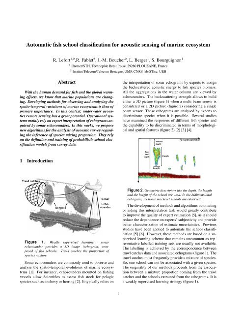
beam sensor. These echograms are analysed by experts to
discriminate species when it is possible. Several studies
have examined the responses of different fish species and
the capability to be discriminated in terms of morphological
and spatial features (figure 2) [2] [3] [4].
Figure 2. Geometric descriptors like the depth, the length
and the height of the school are used. In the bidimensional
echogram, six horse mackerel schools are observed.
The development of methods and algorithms automating
or aiding this interpretation task would greatly contribute
to improve the quality of expert estimation [5], as it should
reduce the dependence on experts’ subjectivity and provide
better characterization of estimate uncertainties. Previous
studies have been applied to automate the school classification
[5] [6]. However, these methods are based on a supervised
learning scheme that remains uncommon as representative
labelled training sets are usually not available.
The labelling is achieved by the correspondence between
trawl catches data and associated echograms (figure 1). The
trawl catches most frequently provide a mixture of species.
So, one school can not be associated with a given species.
The originality of our methods proceeds from the association
between a mixture proportion coming from the trawl
catches and the schools extracted from the echograms. It is
a weakly supervised learning strategy (figure 1).

Figure 3. Example of an oceanographic vessel route in the bay of Biscay. The learning set is composed of echograms obtained
at trawled sites. It provides labelled data necessary to evaluate the classification model. The oceanographic vessel route provides
echograms continuously. All schools in these unlabelled echograms are classed.
The paper is organized as follows. Section 2 presents the
methods and introduces the notations for the probabilistic
model. In section 3 we present the two probabilistic models
based on the conditional model and the Bayesian model.
Performances of these models tested with real and synthetic
data are presented in section 4. Finally, concluding remarks
are given in section 5.
2 Global methods and notation
In this section the weakly supervised learning strategy
and the notation of the probabilistic model are presented.
An oceanographic survey provides two kinds of data set:
NT r echograms associated with NT r trawls catches given
the proportion πn, 1 ≤ n ≤ NT r for each echogram and
NT t echograms without trawl catch (figure 3). The first one
is the training data set that allows us to build our probabilistic
classification model (equation 1). All the non labelled
schools of the second data set are classified independently
using this model.
Considering a probabilistic school-based setting, we aim
at evaluating the likelihood of observed school to be assigned
to a given class. The term class refers to fish species
or group of species. Let us denote by Xnj ∈ R D the observation
vector for the j th school in the n th echogram,
where D is the number of descriptors per schools. For any
2
fish school, we used geometrics and energy descriptors (figure
2) [3] [4], but temporal or geographical descriptors [2]
could be used too. Let us denote by ynjk the value indicating
that the j th school in image n belongs to the class
k. ynjk = 1 if the class is k. ynjk = 0 if the class is different
from k. Introducing in addition the global random
variable πn corresponding to class mixing proportion at the
echogram level provided by the trawl catch, this leads to the
definition of likelihood:
p (ynjk|Xnj, πn) (1)
Note that for the training data set (i.e. for echograms associated
to trawl catches) variable πn is known. The first
step of the method consists in estimating model parameters
Θ (see the section 3 for details) from echograms for which
πn is known (i.e. echograms at trawled sites). In the second
step, the trained model can be applied to any echograms.
To evaluate the performance of the proposed algorithms,
datasets with known ground truth is built. Then, we compare
the class found for each school with the real class.
As there is a lack of mono specific trawl catch, it is hard
to build the ground truth dataset. In practical terms, the
method involves selection of haul having more than 90% of
a determined species. Afterwards the mono specific set of
fish schools is mixed according to the type of echograms

wanted. Then the composition and the species proportion
of each echogram are known that allows us to test classification
algorithms and compare classification results with
real composition. Echograms comprising mixture with one,
two, three, or four classes are simulated. Note that if there is
one specie per echogram, it leads to the supervised case. As
statistical variables must be evaluated from a mixing proportion,
it is easy to understand that the higher is the number
of species in echograms, the less the classification model is
suitable.
In this paper, only 2D data are processed. Simulated
echograms are built with four classes of data either coming
out from the campaign (Sardina: 179 schools, Anchovy:
478 schools, Horse Mackerel: 1859 schools, Blue Whiting:
95 schools) or simulated with the acoustic fish school software
OASIS [7] developed by the IFREMER institute (Anchovy:
1360 schools, Sardina: 1187 schools, Horse Mackerel:
1859 schools). While the fish school simulator provides
big data base for any specie acoustic campaign does
not. For instance, the statistical variables will not be correctly
evaluated with the 95 Blue Whiting schools of the
campaign. Once echograms are built, descriptors are extracted
with a software [8]. 20 descriptors are used: the
depth, the minimum depth, the relative altitude, the minimum
altitude, the backscattering strength, the mean of
acoustic echo, the maximum of acoustic echo, the standard
deviation of acoustic echo, a coefficient describing the
variation of echo, the maximum school height, the mean
school height, the length, the area, the elongation, the fractal
dimension, the circularity, the total energy, the mean energy,
and the index of the amplitude dispersion. Note that
these descriptors are not necessarily discriminative between
them.
3 Models of classification
The two models of classification are presented in this
section. The conditional model and the Bayesian model for
weakly supervised learning have been considered and extended
to our problem. Stated in [9] for binary labelling, an
extension to mixing proportion data is considered.
• The conditional models can be viewed as a probabilistic
setting of discriminative models. In the linear
case, it consists in parametrizing a probabilistic decision
from the signed distance to the decision hyperplane:
p (Ynjk|Xnj, πn) ∝ f(< Wk, Xnj > +bk),
where < Wk, Xnj > +bk = 0 is the equation of the
hyperplane separating the class k from the others and
f is the exponential function. Exponential function
weights the observation as a function of the distance
to the hyperplan. Model parameters Θ = {W, b} are
estimated from a gradient-based minimization of the
3
total proportion estimation error. An minimum error
criterion is considered:
Θ = arg min D(˜πn(Θ), πn) (2)
Θ
n
where ˜πn(Θ) is the vector of the estimated priors of
the acoustic energies relative to the different species
classes: ˜πn(Θ) =
j Enjp (ynj|xnj, Θ), Enj equals
one if these proportions are computed as relative object
occurrences, and D a distance between the observed
and estimated priors. Among the different distances
between likelihood functions, the Battacharrya
distance is chosen. An extension to non-linear models
is proposed here using the kernel trick [10]. The
non linear model consists in a projection of the original
feature space in a new kernel space. Then a Principal
Component Analysis is carried out.
• For the Bayesian model, we develop p (ynjk|Xnj, πn)
according to Bayes relation:
p (ynjk|Xnj, πn) = p(Ynjk|πn)p (Xnj|Ynjk, πn)
p(Ynjl|πn)p (Xnj|Ynjl, πn)
l
(3)
where p(Ynjk|πn) is depending on the proportion πn
into the n th echogram (the expression is given into [9])
and p (Xnj|Ynjk, πn) is a Normal M-mixture distribution
of the form:
p (Xnjk|Ynjk, πn) =
M
m=1
ρk,mN(µk,m, Σk,m) (4)
Where ρk,m is the mixing prior for class k, µk,m and
Σk,m are the Gaussian parameters. Models parameters
Θ = {ρk,m, µk,m, Σk,m} are estimated by an Expectation
Maximization procedure [9]. A diagonal pooled
variance-covariance matrix is chosen to avoid problems
when the inverse matrix is calculated. This implicates
that we suppose that there is no dependence
between descriptors.
4 Results
Figure 4 shows the improvement brought by considering
mixing proportion data for training compared to presence/absence
data [9]. The presence/absence case considers
that the proportion is unknown and replaces it by a binary
value indicating 1 if the class is present in the echogram
and 0 if the class is absent. The correct classification rate is

shown as a function of the complexity of the proportion in
the echogram. A complexity value of zero means that one
class is dominating in the echogram and a complexity of one
means that the proportion is the same for all the classes.
With a simulated database and for the three classification
models, the classification rate of the proportion method is
better compared with the presence/absence method.
Figure 5 shows algorithms performance for real and simulated
data. The rate of correct classification is shown as
a function of the complexity of the training dataset from
mono specific echograms (i.e. in the supervised case) to
three or four class mixture. This allows the behaviour
changes of the methods to be evaluated. The implementation
of the different proportion complexity is done with
a random number computer selection on the mono specific
database. A part of the data base is randomly selected for
the training and the remaining part is used to evaluate the
classification of the trained model. This procedure is carried
out one hundred times and the mean of the correct
classification rates gives the global rate of correct classification.
The higher is the number of species, the less the results
are suitable. Reported results show that the proposed
conditional model outperforms the Bayesian model. The
Bayesian model performance decreases faster when proportions
are more complex. The difference between the linear
and the non linear conditional model is difficult to evaluate
and depends on the dataset but the non linear conditional
model dominates.
Figure 4. Correct classification rate for Simulated
database as a function of the complexity of the class
proportion in the training echogram. Comparison between
the proportion case (dashed line) and the presence/absence
case (solid line) for the three classification
model (Bayesian, Linear conditional and non-linear conditional).
4
Figure 5. Classification performance for real fish school
data (top) and simulated acoustic fish school data (bottom).
The rate of correct classification is reported for the M=5
mixture Bayesian model (solid), the non-linear conditional
model (dashed) with and the linear conditional Model (dotted).
Additional results also point out that correct classification
rate depends on the number of descriptors used for the
classification. Figure 6 presents the correct classification
rate as a function of the complexity when four descriptors
are considered. We picked out from the twenty descriptors
those that are more discriminant. Results show that
the Bayesian model is not robust. Indeed, performance decreases
faster when proportions are more complex but the
rate of correct classification dominates now (more than 10%
for real data) compared with conditional model when the
number of species per echogram is limited. We conclude
that the Expectation Maximization algorithm doesn’t converge
with higher system dimension.
5 Conclusion
This paper considers an original algorithmic method for
studying marine ecosystem. Previous works tried to clas-

Figure 6. Classification performance for real (top) and
simulated (bottom) fish school database using the four descriptors
the most discriminant. The rate of correct classification
is reported for the M=5 mixture Bayesian model
(solid), the non-linear conditional model (dashed) and the
linear conditional Model (dotted) as a function of the proportion
complexity.
sify species using a supervised learning scheme that is not
adapted to oceanographic survey. Our algorithm takes into
account the observation labels coming from trawl catches
give proportion information.
With regards to lack of ground truth, a procedure has
been developed to test and evaluate the classification results.
Before analyze the methods comportments we notice the result
improvement when proportion label is considered compare
to presence/absence label. Performance of the method
depends on the classification model, the origin of database,
and the number of parameters the methods haves to estimate.
Concerning the classification results and considering
all the descriptors, non linear conditional model seems to
be the more adapted to the weakly supervised method. Robustness
and superiority of the model are deduced from the
high level of correct classification and the regularity against
the number of species complexity per echogram. Finaly, we
5
observed that the Bayesian model is sensitive to the number
of descriptors.
References
[1] D. N. MacLennan and E. J. Simmonds, “Fisheries acoustics,” Chapman
& Hall, 1992.
[2] C. Scalabrin and J. Massé, “Acoustic detection of the spatial and temporal
distribution of fish shoals in the bay of biscay,” Aquatic Living
Resources, vol. 6, pp. 269–283, 1993.
[3] C. Scalabrin, N. Diner, A. Weill, A. Hillion, and M.-C. Mouchot,
“Narrowband acoustic identification of monospecific fish shoals,”
ICES Journal of Marine Science, vol. 53, no. 2, pp. 181–188, 1996.
[4] D. MacLennan, P. Fernandes, and D. J., “A consistent approach to
definitions and symbols in fisheries acoustics,” ICES Journal of Marine
Science, vol. 59, pp. 365–369, 2002.
[5] R. Korneliussen, “The bergen echo integrator post-processing system,
with focus on recent improvements.” Fisheries Research, vol.
68(1-3), pp. 159–169, 2004.
[6] J. Haralambous and S. Georgakarakos, “Artificial neural networks as
a tool species identification of fish schools,” ICES Journal of Marine
Science, vol. 53, no. 2, pp. 173–180, 1996.
[7] N. Diner, “Correction on school geometry and density: approach
based on acoustic image simulation.” Aquatic Living Resources, vol.
82(1-3), pp. 211–222, 2001.
[8] N. Diner, A. Weill, J. Coail, and C. J.M., “Ines-movies: a new
acoustic data acquisition and processing system.” ICES CM, vol.
1989/B,45, p. 11 p., 1989.
[9] C. M. Bishop and I. Ulusoy, “Generative versus discriminative methods
for object recognition,” IEEE, CVPR 258-265, 2005.
[10] B. Schölkopf and J. Alexander, “Learning with kernels,” The MIT
Press, 2002.