Method 6020A - US Environmental Protection Agency

METHOD 6020A 

INDUCTIVELY COUPLED PLASMA-MASS SPECTROMETRY 

SW-846 is not intended to be an analytical training manual. Therefore, method 

procedures are written based on the assumption that they will be performed by analysts who are 

formally trained in at least the basic principles of chemical analysis and in the use of the subject 

technology. 

In addition, SW-846 methods, with the exception of required method use for the analysis 

of method-defined parameters, are intended to be guidance methods which contain general 

information on how to perform an analytical procedure or technique which a laboratory can use 

as a basic starting point for generating its own detailed Standard Operating Procedure (SOP), 

either for its own general use or for a specific project application. The performance data 

included in this method are for guidance purposes only, and are not intended to be and must 

not be used as absolute QC acceptance criteria for purposes of laboratory accreditation. 

1.0 SCOPE AND APPLICATION 

1.1 Inductively coupled plasma-mass spectrometry (ICP-MS) is applicable to the 

determination of sub-µg/L concentrations of a large number of elements in water samples and in 

waste extracts or digests (Refs. 1 and 2). When dissolved constituents are required, samples 

must be filtered and acid-preserved prior to analysis. No digestion is required prior to analysis 

for dissolved elements in water samples. Acid digestion prior to filtration and analysis is 

required for groundwater, aqueous samples, industrial wastes, soils, sludges, sediments, and 

other solid wastes for which total (acid-soluble) elements are required. 

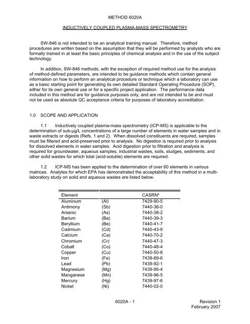
1.2 ICP-MS has been applied to the determination of over 60 elements in various 

matrices. Analytes for which EPA has demonstrated the acceptability of this method in a multilaboratory 

study on solid and aqueous wastes are listed below. 

Element CASRN a 

Aluminum (Al) 7429-90-5 

Antimony (Sb) 7440-36-0 

Arsenic (As) 7440-38-2 

Barium (Ba) 7440-39-3 

Beryllium (Be) 7440-41-7 

Cadmium (Cd) 7440-43-9 

Calcium (Ca) 7440-70-2 

Chromium (Cr) 7440-47-3 

Cobalt (Co) 7440-48-4 

Copper (Cu) 7440-50-8 

Iron (Fe) 7439-89-6 

Lead (Pb) 7439-92-1 

Magnesium (Mg) 7439-95-4 

Manganese (Mn) 7439-96-5 

Mercury (Hg) 7439-97-6 

Nickel (Ni) 7440-02-0 

6020A - 1 Revision 1 

February 2007

Element CASRN a 

Potassium (K) 7440-09-7 

Selenium (Se) 7782-49-2 

Silver (Ag) 7440-22-4 

Sodium (Na) 7440-23-5 

Thallium (Tl) 7440-28-0 

Vanadium (V) 7440-62-2 

Zinc (Zn) 7440-66-6 

a 

Chemical Abstract Service Registry Number 

Acceptability of this method for an element was based upon the multi-laboratory 

performance compared with that of either furnace atomic absorption spectrophotometry or 

inductively coupled plasma-atomic emission spectrometry. It should be noted that one multilaboratory 

study was conducted in 1988 and advances in ICP-MS instrumentation and software 

have been made since that time and additional studies have been added with validation and 

improvements in performance of the method. Performance, in general, exceeds the multilaboratory 

performance data for the listed elements. It is expected that current performance will 

exceed the multi-laboratory performance data for the listed elements (and others) that are 

provided in Sec. 13.0. The lower limit of quantitation and linear ranges will vary with the 

matrices, instrumentation, and operating conditions. In relatively simple matrices, quantitation 

limits will generally be below 0.1 µg/L. Less sensitive elements (like Se and As) and 

desensitized major elements may be 1.0 µg/L or higher. 

1.3 If this method is used to determine any analyte not listed in Sec. 1.2, it is the 

responsibility of the analyst to demonstrate the accuracy and precision of the method in the 

waste to be analyzed. The analyst is always required to monitor potential sources of 

interferences and take appropriate action to ensure data of known quality (see Sec. 9.0). Other 

elements and matrices may be analyzed by this method if performance is demonstrated for the 

analyte of interest, in the matrices of interest, at the concentration levels of interest in the same 

manner as the listed elements and matrices (see Sec. 9.0). 

1.4 An appropriate internal standard is required for each analyte determined by ICP- 

MS. Recommended internal standards are 6 Li, 45 Sc, 89 Y, 103 Rh, 115 In, 159 Tb, 165 Ho, 74 Ge, and 

209 Bi. The lithium internal standard should have an enriched abundance of 6 Li, so that 

interference from lithium native to the sample is minimized. Other elements may need to be 

used as internal standards when samples contain significant native amounts of the 

recommended internal standards. 

1.5 Prior to employing this method, analysts are advised to consult the each 

preparative method that may be employed in the overall analysis (e.g., a 3000 series method) 

for additional information on quality control procedures, development of QC acceptance criteria, 

calculations, and general guidance. Analysts also should consult the disclaimer statement at 

the front of the manual and the information in Chapter Two for guidance on the intended 

flexibility in the choice of methods, apparatus, materials, reagents, and supplies, and on the 

responsibilities of the analyst for demonstrating that the techniques employed are appropriate 

for the analytes of interest, in the matrix of interest, and at the levels of concern. 

In addition, analysts and data users are advised that, except where explicitly specified in a 

regulation, the use of SW-846 methods is not mandatory in response to Federal testing 

requirements. The information contained in this method is provided by EPA as guidance to be 

used by the analyst and the regulated community in making judgments necessary to generate 

results that meet the data quality objectives for the intended application. 


February 2007

1.6 Use of this method is restricted to use by, or under supervision of, properly 

experienced and trained personnel, including spectroscopists who are knowledgeable in the 

recognition and in the correction of spectral, chemical, and physical interferences in ICP-MS. 

Each analyst must demonstrate the ability to generate acceptable results with this method. 

2.0 SUMMARY OF METHOD 

2.1 Prior to analysis, samples should be solubilized or digested using the appropriate 

sample preparation methods (see Chapter Three). When analyzing groundwater or other 

aqueous samples for dissolved constituents, acid digestion is not necessary if the samples are 

filtered and acid preserved prior to analysis (refer to Sec. 1.1). 

2.2 This method describes the multi-elemental determination of analytes by ICP-MS in 

environmental samples. The method measures ions produced by a radio-frequency inductively 

coupled plasma. Analyte species originating in a liquid are nebulized and the resulting aerosol 

is transported by argon gas into the plasma torch. The ions produced by high temperatures are 

entrained in the plasma gas and extracted through a differentially pumped vacuum interface and 

separated on the basis of their mass-to-charge ratio by a mass spectrometer. The ions 

transmitted through the mass spectrometer are quantified by a channel electron multiplier or 

Faraday detector and the ion information is processed by the instrument’s data handling 

system. Interferences must be assessed and valid corrections applied or the data qualified to 

indicate problems. Interference correction must include compensation for background ions 

contributed by the plasma gas, reagents, and constituents of the sample matrix. 

3.0 DEFINITIONS 

Refer to Chapter One, Chapter Three, and the manufacturer's instructions for definitions 

that may be applicable to this procedure. 

4.0 INTERFERENCES 

4.1 Solvents, reagents, glassware, and other sample processing hardware may 

yield artifacts and/or interferences to sample analysis. All these materials must be 

demonstrated to be free from interferences under the conditions of the analysis by analyzing 

method blanks. Specific selection of reagents and purification of solvents by distillation in 

all-glass systems may be necessary. Refer to each method to be used for specific guidance on 

quality control procedures and to Chapter Three for general guidance on the cleaning of 

glassware. Also refer to the preparative methods to be used for discussions on interferences. 

4.2 Isobaric elemental interferences in ICP-MS are caused by isotopes of different 

elements forming atomic ions with the same nominal mass-to-charge ratio (m/z). A data system 

must be used to correct for these interferences. This involves determining the signal for another 

isotope of the interfering element and subtracting the appropriate signal from the analyte 

isotope signal. Since commercial ICP-MS instruments nominally provide unit resolution at 10% 

of the peak height, very high ion currents at adjacent masses can also contribute to ion signals 

at the mass of interest. Although this type of interference is uncommon, it is not easily 

corrected, and samples exhibiting a significant problem of this type could require resolution 

improvement, matrix separation, or analysis using another verified and documented isotope, or 

use of another method. 


February 2007

4.3 Isobaric molecular and doubly-charged ion interferences in ICP-MS are caused by 

ions consisting of more than one atom or charge, respectively. Most isobaric interferences that 

could affect ICP-MS determinations have been identified in the literature (Refs. 3 and 4). 

Examples include 75 ArCl + ion on the 75 As signal and MoO + ions on the cadmium isotopes. While 

the approach used to correct for molecular isobaric interferences is demonstrated below using 

the natural isotope abundances from the literature (Ref. 5), the most precise coefficients for an 

instrument can be determined from the ratio of the net isotope signals observed for a standard 

solution at a concentration providing suitable (

method also provides a method for preconcentration to enhance quantitation limits 

simultaneously with elimination of isobaric interferences. The method relies on chelating resins 

such as imminodiacetate or other appropriate resins and selectively concentrates the elements 

of interest while eliminating interfering elements from the sample matrix. By eliminating the 

elements that are direct isobaric interferences or those that form isobaric interfering molecular 

masses, the mass region is simplified and these interferences can not occur. The method has 

been proven effective for the certification of standard reference materials and validated using 

SRMs (Refs. 13 through 15). The method has the potential to be used on-line or off-line as an 

effective sample preparation method specifically designed to address interference problems. 

4.5 Physical interferences are associated with the sample nebulization and transport 

processes as well as with ion-transmission efficiencies. Nebulization and transport processes 

can be affected if a matrix component causes a change in surface tension or viscosity. 

Changes in matrix composition can cause significant signal suppression or enhancement (Ref. 

9). Dissolved solids can deposit on the nebulizer tip of a pneumatic nebulizer and on the 

interface skimmers (reducing the orifice size and the instrument performance). Total solid 

levels below 0.2% (2,000 mg/L) are recommended (Ref. 10) to minimize solid deposition. An 

internal standard can be used to correct for physical interferences, if it is carefully matched to 

the analyte so that the two elements are similarly affected by matrix changes (Ref. 11). When 

intolerable physical interferences are present in a sample, a significant suppression of the 

internal standard signals (to less than 30% of the signals in the calibrations standard) will be 

observed. Dilution of the sample fivefold (1+4) will usually eliminate the problem (see Sec. 9.5). 

4.6 Memory interferences or carry-over can occur when there are large concentration 

differences between samples or standards which are analyzed sequentially. Sample deposition 

on the sampler and skimmer cones, spray chamber design, and the type of nebulizer affect the 

extent of observed memory interferences. The rinse period between samples must be long 

enough to eliminate significant memory interference. 

5.0 SAFETY 

5.1 This method does not address all safety issues associated with its use. The 

laboratory is responsible for maintaining a safe work environment and a current awareness file 

of OSHA regulations regarding the safe handling of the chemicals specified in this method. A 

reference file of material safety data sheets (MSDSs) should be available to all personnel 

involved in these analyses. 

5.2 Concentrated nitric and hydrochloric acids are moderately toxic and extremely 

irritating to skin and mucus membranes. Use these reagents in a hood and if eye or skin 

contact occurs, flush with large volumes of water. Always wear safety glasses or a shield for 

eye protection when working with these reagents. Hydrofluoric acid is a very toxic acid and 

penetrates the skin and tissues deeply if not treated immediately. Injury occurs in two stages; 

first, by hydration that induces tissue necrosis and then by penetration of fluoride ions deep into 

the tissue and by reaction with calcium. Boric acid and other complexing reagents and 

appropriate treatment agents should be administered immediately. Consult appropriate safety 

literature and have the appropriate treatment materials readily available prior to working with 

this acid. See Method 3052 for specific suggestions for handling hydrofluoric acid from a safety 

and an instrument standpoint. 

5.3 Many metal salts are extremely toxic if inhaled or swallowed. Extreme care must 

be taken to ensure that samples and standards are handled properly and that all exhaust gases 

are properly vented. Wash hands thoroughly after handling. 


February 2007

5.4 The acidification of samples containing reactive materials may result in the release 

of toxic gases, such as cyanides or sulfides. For this reason, the acidification and digestion of 

samples should be performed in an approved fume hood. 

6.0 EQUIPMENT AND SUPPLIES 

6.1 Inductively coupled plasma-mass spectrometer -- A system capable of providing 

resolution, better than or equal to 1.0 amu at 10% peak height is required. The system must 

have a mass range from at least 6 to 240 amu and a data system that allows corrections for 

isobaric interferences and the application of the internal standard technique. Use of a 

mass-flow controller for the nebulizer argon and a peristaltic pump for the sample solution is 

recommended. 

6.2 Argon gas supply -- High-purity grade (99.99%). 

7.0 REAGENTS AND STANDARDS 

7.1 Reagent- or trace metals-grade chemicals must be used in all tests. Unless 

otherwise indicated, it is intended that all reagents conform to the specifications of the 

Committee on Analytical Reagents of the American Chemical Society, where such 

specifications are available. Other grades may be used, provided it is first ascertained that the 

reagent is of sufficiently high purity to permit its use without lessening the accuracy of the 

determination. 

7.2 Acids used in the preparation of standards and for sample processing must be of 

high purity. Redistilled acids are recommended because of the high sensitivity of ICP-MS. 

Nitric acid at less than 2% (v/v) is required for ICP-MS to minimize damage to the interface and 

to minimize isobaric molecular-ion interferences with the analytes. Many more molecular-ion 

interferences are observed when hydrochloric and sulfuric acids are used (Refs. 3 and 4). 

Concentrations of antimony and silver between 50-500 µg/L require 1% (v/v) HCl for stability; for 

concentrations above 500 µg/L Ag, additional HCl will be needed. Consequently, accuracy of 

analytes requiring significant chloride molecular ion corrections (such as As and V) will degrade. 

7.3 Reagent water -- All references to water in the method refer to reagent water, 

unless otherwise specified. Reagent water must be free of interferences. 

7.4 Standard stock solutions for each analyte may be purchased or prepared from 

ultra-high purity grade chemicals or metals (99.99 or greater purity). See Method 6010 for 

instructions on preparing standard solutions from solids. 

7.4.1 Bismuth internal standard stock solution (1 mL = 100 µg of Bi) -- Dissolve 

0.1115 g of Bi 2O 3 in a minimum amount of dilute HNO 3. Add 10 mL of conc. HNO 3 and 

dilute to 1,000 mL with reagent water. 

7.4.2 Germanium internal standard stock solution (1 mL = 100 µg of Ge) -- 

Dissolve 0.2954 g of GeCl 4 in a minimum amount of dilute HNO 3. Add 10 mL of conc. 

HNO 3 and dilute to 1,000 mL with reagent water. 

7.4.3 Holmium internal standard stock solution (1 mL = 100 µg of Ho) -- 

Dissolve 0.1757 g of Ho 2(CO 3) 2C5H 2O in 10 mL of reagent water and 10 mL of HNO 3. After 

dissolution is complete, warm the solution to degas. Add 10 mL conc. of HNO 3 and dilute 

to 1,000 mL with reagent water. 


February 2007

7.4.4 Indium internal standard stock solution (1 mL = 100 µg of In) -- Dissolve 

0.1000 g of indium metal in 10 mL of conc. HNO 3. Dilute to 1,000 mL with reagent water. 

7.4.5 Lithium internal standard stock solution (1 mL = 100 µg of 6 Li) -- Dissolve 

0.6312 g of 95-atom-% 6 Li, Li 2CO 3 in 10 mL of reagent water and 10 mL of HNO 3. After 

dissolution is complete, warm the solution to degas. Add 10 mL conc. of HNO 3 and dilute 

to 1,000 mL with reagent water. 

7.4.6 Rhodium internal standard stock solution (1 mL = 100 µg of Rh) -- 

Dissolve 0.3593 g of ammonium hexachlororhodate (III) (NH 4) 3RhCl 6 in 10 mL reagent 

water. Add 100 mL of conc. HCl and dilute to 1,000 mL with reagent water. 

7.4.7 Scandium internal standard stock solution (1 mL = 100 µg of Sc) -- 

Dissolve 0.15343 g of Sc 2O 3 in 10 mL (1+1) of hot HNO 3. Add 5 mL of conc. HNO 3 and 

dilute to 1,000 mL with reagent water. 

7.4.8 Terbium internal standard stock solution (1 mL = 100 µg of Tb) -- Dissolve 

0.1828 g of Tb 2(CO 3) 3C5H 2O in 10 mL (1+1) of HNO 3. After dissolution is complete, warm 

the solution to degas. Add 5 mL of conc. HNO 3 and dilute to 1,000 mL with reagent water. 

7.4.9 Yttrium internal standard stock solution (1 mL = 100 µg of Y) -- Dissolve 

0.2316 g of Y 2(CO 3) 3C3H 2O in 10 mL (1+1) of HNO 3. Add 5 mL conc. of HNO 3 and dilute to 

1,000 mL with reagent water. 

7.4.10 Titanium interference stock solution (1 mL = 100 µg of Ti) -- Dissolve 

0.4133 g of (NH 4) 2TiF 6 in reagent water. Add 2 drops of conc. HF and dilute to 1,000 mL 

with reagent water. 

7.4.11 Molybdenum interference stock solution (1 mL = 100 µg of Mo) -- 

Dissolve 0.2043 g of (NH 4) 2MoO 4 in reagent water. Dilute to 1,000 mL with reagent water. 

7.4.12 Gold preservative stock solution for mercury (1 mL = 100 µg) -- 

Recommend purchasing as high purity prepared solution of AuCl 3 in dilute hydrochloric 

acid matrix. 

7.5 Mixed calibration standard solutions are prepared by diluting the stock-standard 

solutions to levels in the linear range for the instrument in a solvent consisting of 1% (v/v) HNO 3 

in reagent water. The calibration standard solutions must contain a suitable concentration of an 

appropriate internal standard for each analyte. Internal standards may be added on-line at the 

time of analysis using a second channel of the peristaltic pump and an appropriate mixing 

manifold. Generally, an internal standard should be no more than 50 amu removed from the 

analyte. Recommended internal standards include 6 Li, 45 Sc, 89 Y, 103 Rh, 115 In, 159 Tb, 169 Ho, 74 Ge 

and 209 Bi. Prior to preparing the mixed standards, each stock solution must be analyzed 

separately to determine possible spectral interferences or the presence of impurities. Care 

must be taken when preparing the mixed standards to ensure that the elements are compatible 

and stable together. Transfer the mixed standard solutions to freshly acid-cleaned FEP 

fluorocarbon or previously unused polyethylene or polypropylene bottles for storage. For all 

intermediate and working standards, especially low level standards (i.e.,

possible contamination resulting from either the reagents (acids) or the equipment used during 

sample processing including filtration. The rinse blank is used to flush the system between all 

samples and standards. 

7.6.1 The calibration blank consists of the same concentration(s) of the same 

acid(s) used to prepare the final dilution of the calibrating solutions of the analytes [often 

1% HNO 3 (v/v) in reagent water] along with the selected concentrations of internal 

standards such that there is an appropriate internal standard element for each of the 

analytes. Use of HCl for antimony and silver is cited in Sec. 7.2. 

7.6.2 The method blank must contain all of the reagents in the same volumes 

as used in the processing of the samples. The method blank must be carried through the 

complete procedure and contain the same acid concentration in the final solution as the 

sample solution used for analysis (refer to Sec. 9.9). 

7.6.3 The rinse blank consists of 1 to 2% of HNO 3 (v/v) in reagent water. 

Prepare a sufficient quantity to flush the system between standards and samples. If 

mercury is to be analyzed, the rinse blank should also contain 2 µg/mL (ppm) of AuCl 3 

solution. 

7.7 The interference check solution (ICS) is prepared to contain known concentrations 

of interfering elements that will demonstrate the magnitude of interferences and provide an 

adequate test of any corrections. Chloride in the ICS provides a means to evaluate software 

corrections for chloride-related interferences such as 35 Cl 16 O + on 51 V + and 40 Ar 35 Cl + on 75 As + . 

Iron is used to demonstrate adequate resolution of the spectrometer for the determination of 

manganese. Molybdenum serves to indicate oxide effects on cadmium isotopes. The other 

components are present to evaluate the ability of the measurement system to correct for various 

molecular-ion isobaric interferences. The ICS is used to verify that the interference levels are 

corrected by the data system within quality control limits. 

NOTE: The final ICS solution concentrations in Table 1 are intended to evaluate corrections 

for known interferences on only the analytes in Sec. 1.2. If this method is used to 

determine an element not listed in Sec. 1.2, the analyst should modify the ICS 

solutions, or prepare an alternative ICS solution, to allow adequate verification of 

correction of interferences on the unlisted element (see Sec. 9.7). 

7.7.1 These solutions must be prepared from ultra-pure reagents. They can be 

obtained commercially or prepared by the following procedure. 

7.7.1.1 Mixed ICS solution I may be prepared by adding 13.903 g of 

Al(NO 3) 3C9H 2O, 2.498 g of CaCO 3 (dried at 180 EC for 1 hr before weighing), 

1.000 g of Fe, 1.658 g of MgO, 2.305 g of Na 2CO 3, and 1.767 g of K 2CO 3 to 25 mL 

of reagent water. Slowly add 40 mL of (1+1) HNO 3. After dissolution is complete, 

warm the solution to degas. Cool and dilute to 1,000 mL with reagent water. 

7.7.1.2 Mixed ICS solution II may be prepared by slowly adding 

7.444 g of 85 % H 3PO 4, 6.373 g of 96% H 2SO 4, 40.024 g of 37% HCl, and 10.664 g 

of citric acid C 6O 7H 8 to 100 mL of reagent water. Dilute to 1,000 mL with reagent 

water. 

7.7.1.3 Mixed ICS solution III may be prepared by adding 1.00 mL 

each of 100-µg/mL arsenic, cadmium, selenium, chromium, cobalt, copper, 

manganese, nickel, silver, vanadium, and zinc stock solutions to about 50 mL of 


February 2007

eagent water. Add 2.0 mL of concentrated HNO 3, and dilute to 100.0 mL with 

reagent water. 

7.7.1.4 Working ICS solutions 

7.7.1.4.1 ICS-A may be prepared by adding 10.0 mL of 

mixed ICS solution I (Sec. 7.7.1.1), 2.0 mL each of 100-µg/mL titanium 

stock solution (Sec. 7.4.9) and molybdenum stock solution (Sec. 7.4.10), 

and 5.0 mL of mixed ICS solution II (Sec. 7.7.1.2). Dilute to 100 mL with 

reagent water. ICS solution A must be prepared fresh weekly. 

7.7.1.4.2 ICS-AB may be prepared by adding 10.0 mL of 

mixed ICS solution I (Sec. 7.7.1.1), 2.0 mL each of 100-µg/mL titanium 

stock solution (Sec. 7.4.9) and molybdenum stock solution (Sec. 7.4.10), 

5.0 mL of mixed ICS solution II (Sec. 7.7.1.2), and 2.0 mL of mixed ICS 

solution III (Sec. 7.7.1.3). Dilute to 100 mL with reagent water. Although 

the ICS solution AB must be prepared fresh weekly, the analyst should be 

aware that the solution may precipitate silver more quickly. 

7.8 The initial calibration verification (ICV) standard is prepared by the analyst (or a 

purchased second source reference material) by combining compatible elements from a 

standard source different from that of the calibration standard, and at concentration near the 

midpoint of the calibration curve (see Sec. 10.4.3 for use). This standard may also be 

purchased. 

7.9 The continuing calibration verification (CCV) standard should be prepared in the 

same acid matrix using the same standards used for calibration, at a concentration near the 

mid-point of the calibration curve (see Sec. 10.4.4 for use). 

7.10 Mass spectrometer tuning solution. A solution containing elements representing all 

of the mass regions of interest (for example, 10 µg/L of Li, Co, In, and Tl) must be prepared to 

verify that the resolution and mass calibration of the instrument are within the required 

specifications (see Sec. 10.2). This solution is also used to verify that the instrument has 

reached thermal stability (see Sec. 11.4). 

8.0 SAMPLE COLLECTION, PRESERVATION, AND STORAGE 

8.1 See the introductory material in Chapter Three, "Inorganic Analytes." 

8.2 Only polyethylene or fluorocarbon (TFE or PFA) containers are recommended for 

use in this method. 

9.0 QUALITY CONTROL 

9.1 Refer to Chapter One for additional guidance on quality assurance (QA) and 

quality control (QC) protocols. When inconsistencies exist between QC guidelines, methodspecific 

QC criteria take precedence over both technique-specific criteria and those criteria 

given in Chapter One, and technique-specific QC criteria take precedence over the criteria in 

Chapter One. Any effort involving the collection of analytical data should include development 

of a structured and systematic planning document, such as a Quality Assurance Project Plan 

(QAPP) or a Sampling and Analysis Plan (SAP), which translates project objectives and 

specifications into directions for those that will implement the project and assess the results. 


February 2007

Each laboratory should maintain a formal quality assurance program. The laboratory should 

also maintain records to document the quality of the data generated. All data sheets and 

quality control data should be maintained for reference or inspection. 

9.2 Refer to a 3000 series method (Method 3005, 3010, 3015, 3031, 3040, 3050, 

3051, or 3052) for appropriate QC procedures to ensure the proper operation of the various 

sample preparation techniques. 

9.3 Instrument detection limits (IDLs) are a useful tool to evaluate the instrument noise 

level and response changes over time for each analyte from a series of reagent blank analyses 

to obtain a calculated concentration. They are not to be confused with the lower limits of 

quantitation, nor should they be used in establishing this limit. It may be helpful to compare the 

calculated IDLs to the established lower limit of quantitation, however, it should be understood 

that the lower limit of quantitation needs to be verified according to the guidance in Sec. 10.2.3. 

IDLs in µg/L can be estimated by calculating the average of the standard deviations of 

three runs on three non-consecutive days from the analysis of a reagent blank solution with 

seven consecutive measurements per day. Each measurement should be performed as though 

it were a separate analytical sample (i.e., each measurement must be followed by a rinse and/or 

any other procedure normally performed between the analysis of separate samples). IDLs 

should be determined at least every three months or at a project-specific designated frequency 

and kept with the instrument log book. Refer to Chapter One for additional guidance. 

9.4 Initial demonstration of proficiency 

Each laboratory must demonstrate initial proficiency with each sample preparation (a 3000 

series method) and determinative method combination it utilizes by generating data of 

acceptable accuracy and precision for target analytes in a clean matrix. If an autosampler is 

used to perform sample dilutions, before using the autosampler to dilute samples, the laboratory 

should satisfy itself that those dilutions are of equivalent or better accuracy than is achieved by 

an experienced analyst performing manual dilutions. The laboratory must also repeat the 

demonstration of proficiency whenever new staff members are trained or significant changes in 

instrumentation are made. 

9.5 Dilute and reanalyze samples that exceed the linear dynamic range or use an 

alternate, less sensitive calibration for which quality control data are already established. 

9.6 The intensities of all internal standards must be monitored for every analysis. If 

the intensity of any internal standard in a sample falls below 70% of the intensity of that internal 

standard in the initial calibration standard, a significant matrix effect must be suspected. As an 

example, if the initial calibration internal standard response is 100,000 cps, anything below 

70,000 cps in the sample would be unacceptable. Under these conditions, the established 

lower limit of quantitation has degraded and the correction ability of the internal standardization 

technique becomes questionable. The following procedure is followed -- First, make sure the 

instrument has not drifted by observing the internal standard intensities in the nearest clean 

matrix (calibration blank, Sec. 7.6.1). If the low internal standard intensities are also seen in the 

nearest calibration blank, terminate the analysis, correct the problem, recalibrate, verify the new 

calibration, and reanalyze the affected samples. If drift has not occurred, matrix effects need to 

be removed by dilution of the affected sample. The sample must be diluted fivefold (1+4) and 

reanalyzed with the addition of appropriate amounts of internal standards. If the first dilution 

does not eliminate the problem, this procedure must be repeated until the internal-standard 

intensities rise to the minimum 70% limit. Reported results must be corrected for all dilutions. 


February 2007

9.7 To obtain analyte data of known quality, it is necessary to measure more than the 

analytes of interest in order to apply corrections or to determine whether interference 

corrections are necessary. For example, tungsten oxide moleculars can be very difficult to 

distinguish from mercury isotopes. If the concentrations of interference sources (such as C, Cl, 

Mo, Zr, W) are such that, at the correction factor, the analyte is less than the limit of 

quantification and the concentration of interferents are insignificant, then the data may go 

uncorrected. Note that monitoring the interference sources does not necessarily require 

monitoring the interferant itself, but that a molecular species may be monitored to indicate the 

presence of the interferent. When correction equations are used, all QC criteria must also be 

met. Extensive QC for interference corrections are required at all times. The monitored masses 

must include those elements whose hydrogen, oxygen, hydroxyl, chlorine, nitrogen, carbon and 

sulfur molecular ions could impact the analytes of interest. Unsuspected interferences may be 

detected by adding pure major matrix components to a sample to observe any impact on the 

analyte signals. When an interference source is present, the sample elements impacted must 

be flagged to indicate (a) the percentage interference correction applied to the data or (b) an 

uncorrected interference by virtue of the elemental equation used for quantitation. The isotope 

proportions for an element or molecular-ion cluster provide information useful for quality 

assurance. 

NOTE: Only isobaric elemental, molecular, and doubly charged interference corrections 

which use the observed isotopic-response ratios or parent-to-oxide ratios (provided 

an oxide internal standard is used as described in Sec. 4.2) for each instrument 

system are acceptable corrections for use in Method 6020. 

9.8 For each batch of samples processed, at least one method blank must be carried 

throughout the entire sample preparation and analytical process, as described in Chapter One. 

A method blank is prepared by using a volume or weight of reagent water at the volume or 

weight specified in the preparation method, and then carried through the appropriate steps of 

the analytical process. These steps may include, but are not limited to, prefiltering, digestion, 

dilution, filtering, and analysis. If the method blank does not contain target analytes at a level 

that interferes with the project-specific DQOs, then the method blank would be considered 

acceptable. 

In the absence of project-specific DQOs, if the blank is less than 10% of the lower limit of 

quantitation check sample concentration, less than 10% of the regulatory limit, or less than 10% 

of the lowest sample concentration for each analyte in a given preparation batch, whichever is 

greater, then the method blank is considered acceptable. If the method blank cannot be 

considered acceptable, the method blank should be re-run once, and if still unacceptable, then 

all samples after the last acceptable method blank should be reprepared and reanalyzed along 

with the other appropriate batch QC samples. These blanks will be useful in determining if 

samples are being contaminated. If the method blank exceeds the criteria, but the samples are 

all either below the reporting level or below the applicable action level or other DQOs, then the 

sample data may be used despite the contamination of the method blank. 

9.9 Laboratory control sample (LCS) 

For each batch of samples processed, at least one LCS must be carried throughout the 

entire sample preparation and analytical process. The laboratory control samples should be 

spiked with each analyte of interest at the project-specific action level or, when lacking projectspecific 

action levels, at approximately mid-point of the linear dynamic range. Acceptance 

criteria should either be defined in the project-specifc planning documents or set at a laboratory 

derived limit developed through the use of historical analyses. In the absence of project-specific 

or historical data generated criteria, this limit should be set at ± 20% of the spiked value. 

Acceptance limits derived from historical data should be no wider that ± 20%. If the laboratory 

control sample is not acceptable, then the laboratory control sample should be re-run once and, 


February 2007

if still unacceptable, all samples after the last acceptable laboratory control sample should be 

reprepared and reanalyzed. 

Concurrent analyses of standard reference materials (SRMs) containing known amounts 

of analytes in the media of interest are recommended and may be used as an LCS. For solid 

SRMs, 80 - 120% accuracy may not be achievable and the manufacturer’s established 

acceptance criterion should be used for soil SRMs. 

9.10 Matrix spike, unspiked duplicate, or matrix spike duplicate (MS/Dup or MS/MSD) 

Documenting the effect of the matrix, for a given preparation batch consisting of similar 

sample characteristics, should include the analysis of at least one matrix spike and one 

duplicate unspiked sample or one matrix spike/matrix spike duplicate pair. The decision on 

whether to prepare and analyze duplicate samples or a matrix spike/matrix spike duplicate must 

be based on a knowledge of the samples in the sample batch or as noted in the project-specific 

planning documents. If samples are expected to contain target analytes, then laboratories may 

use one matrix spike and a duplicate analysis of an unspiked field sample. If samples are not 

expected to contain target analytes, laboratories should use a matrix spike and matrix spike 

duplicate pair. 

For each batch of samples processed, at least one MS/Dup or MS/MSD sample set should 

be carried throughout the entire sample preparation and analytical process as described in 

Chapter One. MS/MSDs are intralaboratory split samples spiked with identical concentrations 

of each analyte of interest. The spiking occurs prior to sample preparation and analysis. An 

MS/Dup or MS/MSD is used to document the bias and precision of a method in a given sample 

matrix. 

Refer to Chapter One for definitions of bias and precision, and for the proper data 

reduction protocols. MS/MSD samples should be spiked at the same level, and with the same 

spiking material, as the corresponding laboratory control sample that is at the project-specific 

action level or, when lacking project-specific action levels, at approximately mid-point of the 

linear dynamic range. Acceptance criteria should either be defined in the project-specifc 

planning documents or set at a laboratory-derived limit developed through the use of historical 

analyses per matrix type analyzed. In the absence of project-specific or historical data 

generated criteria, these limits should be set at ± 25% of the spiked value for accuracy and 20 

relative percent difference (RPD) for precision. Acceptance limits derived from historical data 

should be no wider that ± 25% for accuracy and 20% for precision. Refer to Chapter One for 

additional guidance. If the bias and precision indicators are outside the laboratory control limits, 

if the percent recovery is less than 75% or greater than 125%, or if the relative percent 

difference is greater than 20%, then the interference test discussed in Sec. 9.11 should be 

conducted. 

9.10.1 The relative percent difference between spiked matrix duplicate or 

unspiked duplicate determinations is to be calculated as follows: 

where: 

RPD ' 

RPD = relative percent difference. 

*D 1 & D 2 * 

*D1 % D2 * 

2 

× 100 


February 2007

D 1 = first sample value. 

D 2 = second sample value (spiked or unspiked duplicate). 

9.10.2 The spiked sample or spiked duplicate sample recovery should be within 

± 25% of the actual value, or within the documented historical acceptance limits for each 

matrix. 

9.11 If less than acceptable accuracy and precision data are generated, additional 

quality control tests (Secs. 9.11.1 and 9.11.2) are recommended prior to reporting concentration 

data for the elements in this method. At a minimum these tests should be performed with each 

batch of samples prepared/analyzed with corresponding unacceptable data quality results. 

These test will then serve to ensure that neither positive nor negative interferences are affecting 

the measurement of any of the elements or distorting the accuracy of the reported values. If 

matrix effects are confirmed, the laboratory should consult with the data user when feasible for 

possible corrective actions which may include the use of alternative or modified test procedures 

so that the analysis is not impacted by the same interference. 

9.11.1 Post digestion spike addition 

If the MS/MSD recoveries are unacceptable, the same sample from which the 

MS/MSD aliquots were prepared should also be spiked with a post digestion spike. 

Otherwise another sample from the same preparation should be used as an alternative. 

An analyte spike is added to a portion of a prepared sample, or its dilution, and should be 

recovered to within 80% to 120% of the known value. The spike addition should produce 

a minimum level of 10 times and a maximum of 100 times the lower limit of quantitation. If 

this spike fails, then the dilution test (Sec. 9.11.2) should be run on this sample. If both 

the MS/MSD and the post digestion spike fail, then matrix effects are confirmed. 

9.11.2 Dilution test 

If the analyte concentration is sufficiently high (minimally, a factor of 10 above the 

lower limit of quantitation after dilution), an analysis of a 1:5 dilution should agree within ± 

10% of the original determination. If not, then a chemical or physical interference effect 

should be suspected. 

9.12 Ultra-trace analysis requires the use of clean chemistry preparation and analysis 

techniques. Several suggestions for minimizing analytical blank contamination are provided in 

Chapter Three. 

10.0 CALIBRATION AND STANDARDIZATION 

10.1 Set up the instrument with proper operating parameters established as detailed 

below. The instrument should be allowed to become thermally stable before beginning (usually 

requiring at least 30 min of operation prior to calibration). For operating conditions, the analyst 

should follow the instructions provided by the instrument manufacturer. 

10.2 Conduct mass calibration and resolution checks in the mass regions of interest. 

The mass calibration and resolution parameters are required criteria which must be met prior to 

any samples being analyzed. If the mass calibration differs more than 0.1 amu from the true 

value, then the mass calibration must be adjusted to the correct value. The resolution must also 

be verified to be less than 0.9 amu full width at 10% peak height. 


February 2007

10.2.1 Before using this procedure to analyze samples, data should be available 

documenting the initial demonstration of performance. The required data should 

document the determination of the linear dynamic ranges; a demonstration of the desired 

method sensitivity and instrument detection limits; and the determination and verification 

of the appropriate correction equations or other routines for correcting spectral 

interferences. These data should be generated using the same instrument, operating 

conditions, and calibration routine to be used for sample analysis. These data should be 

kept on file and be available for review by the data user or auditor. 

10.2.2 Sensitivity, instrumental detection limit, precision, linear dynamic range, 

and interference corrections need to be established for each individual target analyte on 

each particular instrument. All measurements (both target analytes and constituents 

which interfere with the target analytes) need to be within the instrument linear range 

where the correction equations are valid. 

10.2.3 The lower limits of quantitation should be established for all isotope 

masses utilized for each type of matrix analyzed and for each preparation method used 

and for each instrument. These limits are considered the lowest reliable laboratory 

reporting concentrations and should be established from the lower limit of quantitation 

check sample and then confirmed using either the lowest calibration point or from a lowlevel 

calibration check standard. 

10.2.3.1 Lower limit of quantitation check sample 

The lower limit of quantitation check (LLQC) sample should be analyzed 

after establishing the lower laboratory reporting limits and on an as needed basis 

to demonstrate the desired detection capability. Ideally, this check sample and the 

low-level calibration verification standard will be prepared at the same 

concentrations with the only difference being the LLQC sample is carried through 

the entire preparation and analytical procedure. Lower limits of quantitation are 

verified when all analytes in the LLQC sample are detected within ± 30% of their 

true value. This check should be used to both establish and confirm the lowest 

quantitation limit. 

10.2.3.2 The lower limits of quantitation determination using reagent 

water represents a best case situation and does not represent possible matrix 

effects of real-world samples. For the application of lower limits of quantitation on 

a project-specific basis with established data quality objectives, low-level matrixspecific 

spike studies may provide data users with a more reliable indication of the 

actual method sensitivity and minimum detection capabilities. 

10.2.4 Specific recommended isotopes for the analytes noted in Sec. 1.2 are 

provided in Table 2. Other isotopes may be substituted if they can provide the needed 

sensitivity and are corrected for spectral interference. Because of differences among 

various makes and models of mass spectrometers, specific instrument operating 

conditions cannot be provided. The instrument and operating conditions utilized for 

determination must be capable of providing data of acceptable quality for the specific 

project and data user. The analyst should follow the instructions provided by the 

instrument manufacturer unless other conditions provide similar or better performance for 

a given task. 

10.3 All masses which could affect data quality should be monitored to determine 

potential effects from matrix components on the analyte peaks. The recommended isotopes to 

be monitored are listed in Table 2. 


February 2007

10.4 All analyses require that a calibration curve be prepared to cover the appropriate 

concentration range based on the intended application and prior to establishing the linear 

dynamic range. Usually, this means the preparation of a calibration blank and mixed calibration 

standard solutions (Sec. 7.5), the highest of which would not exceed the anticipated linear 

dynamic range of the instrument. Check the instrument standardization by analyzing 

appropriate QC samples as follows. 

10.4.1 Individual or mixed calibration standards should be prepared from known 

primary stock standards every six months to one year as needed based on the 

concentration stability as confirmed from the ICV analyses. The analysis of the ICV, which 

is prepared from a source independent of the calibration standards, is necessary to verify 

the instrument performance once the system has been calibrated for the desired target 

analytes. It is recommended that the ICV solution be obtained commercially as a certified 

traceable reference material such that an expiration date can be assigned. Alternately, 

the ICV solution can be prepared from an independent source on an as needed basis 

depending on the ability to meet the calibration verification criteria. If the ICV analysis is 

outside of the acceptance criteria, at a minimum the calibration standards must be 

prepared fresh and the instrument recalibrated prior to beginning sample analyses. 

Consideration should also be given to preparing fresh ICV standards if the new calibration 

cannot be verified using the existing ICV standard. 

NOTE: This method describes the use of both a low-level and mid-level ICV standard 

analysis. For purposes of verifying the initial calibration, only the mid-level ICV 

needs to be prepared from a source other than the calibration standards. 

10.4.1.1 The calibration standards should be prepared using the same 

type of acid or combination of acids and at similar concentrations as will result in 

the samples following processing. 

10.4.1.2 The response of the calibration blank should be less than the 

response of the typical laboratory lower limit of quantitation for each desired target 

analyte. Additionally, if the calibration blank response or continuing calibration 

blank verification is used to calculate a theoretical concentration, this value should 

be less than the level of acceptable blank contamination as specified in the 

approved quality assurance project planning documents. If this is not the case, the 

reason for the out-of-control condition must be found and corrected, and the 

sample analyses may not proceed or the previous ten samples need to be 

reanalyzed. 

10.4.2 For the initial and daily instrument operation, calibrate the system 

according to the instrument manufacturer’s guidelines using the mixed calibration 

standards as noted in Sec. 7.5. The calibration curve should be prepared daily with a 

minimum of a calibration blank and a single standard at the appropriate concentration to 

effectively outline the desired quantitation range. Flush the system with the rinse blank 

(Sec. 7.6.3) between each standard solution. Use the average of at least three 

integrations for both calibration and sample analyses. The resulting curve should then be 

verified with mid-level and low-level initial calibration verification standards as outlined in 

Sec. 10.4.3. 

Alternatively, the calibration curve can be prepared daily with a minimum of a 

calibration blank and three non-zero standards that effectively bracket the desired sample 

concentration range. If low-level as compared to mid- or high-level sample concentrations 

are expected, the calibration standards should be prepared at the appropriate 

concentrations in order to demonstrate the instrument linearity within the anticipated 


February 2007

sample concentration range. For all multi-point calibration scenarios, the lowest non-zero 

standard concentration should be considered the lower limit of quantitation. 

NOTE: Regardless of whether the instrument is calibrated using only a minimum number 

of standards or with a multi-point curve, the upper limit of the quantitation range 

may exceed the highest concentration calibration point and can be defined as the 

"linear dynamic" range, while the lower limit can be identified as the "lower limit of 

quantitation limit" (LLQL) and will be either the concentration of the lowest 

calibration standard (for multi-point curves) or the concentration of the low level 

ICV/CCV check standard. Results reported outside these limits would not be 

recommended unless they are qualified as estimated. See Sec. 10.4.4 for 

recommendations on how to determine the linear dynamic range, while the 

guidance in this section and Sec. 10.4.3 provide options for defining the lower 

limit of quantitation. 

10.4.2.1 To be considered acceptable, the calibration curve should 

have a correlation coefficient greater than or equal to 0.998. When using a multipoint 

calibration curve approach, every effort should be made to attain an 

acceptable correlation coefficient based on a linear response for each desired 

target analyte. If the recommended linear response cannot be attained using a 

minimum of three non-zero calibration standards, consideration should be given to 

adding more standards, particularly at the lower concentrations, in order to better 

define the linear range and the lower limit of quantitation. Conversely, the extreme 

upper and lower calibration points may be removed from the multi-point curve as 

long as three non-zero points remain such that the linear range is narrowed and 

the non-linear upper and/or lower portions are removed. As with the single point 

calibration option, the multi-point calibration should be verified with both a mid- and 

low-level ICV standard analysis using the same 90 - 110% and 70 - 130% 

acceptance criteria, respectively. 

10.4.2.2 Many instrument software packages allow multi-point 

calibration curves to be "forced" through zero. It is acceptable to use this feature, 

provided that the resulting calibration meets the acceptance criteria, and can be 

verified by acceptable QC results. Forcing a regression through zero should NOT 

be used as a rationale for reporting results below the calibration range defined by 

the lowest standard in the calibration curve. 

10.4.3 After initial calibration, the calibration curve should be verified by use of 

an initial calibration verification (ICV) standard analysis. At a minimum, the ICV standard 

should be prepared from an independent (second source) material at or near the midrange 

of the calibration curve. The acceptance criteria for this mid-range ICV standard 

should be ±10% of its true value. Additionally, a low-level initial calibration verification 

(LLICV) standard should be prepared, using the same source as the calibration standards, 

at a concentration expected to be the lower limit of quantitation. The suggested 

acceptance criteria for the LLICV is ±30% of its true value. Quantitative sample analyses 

should not proceed for those analytes that fail the second source standard initial 

calibration verification, with the exception that analyses may continue for those analytes 

that fail the criteria with an understanding these results should be qualified and would be 

considered estimated values. Once the calibration acceptance criteria is met, either the 

lowest calibration standard or the LLICV concentration can be used to demonstrate the 

lower limit of quantitation and sample results should not be quantitated below this lowest 

standard. In some cases depending on the stated project data quality objectives, it may 

be appropriate to report these results as estimated, however, they should be qualified by 

noting the results are below the lower limit of quantitation. Therefore, the laboratory’s 


February 2007

quantitation limit cannot be reported lower than either the LLICV standard used for the 

single point calibration option or the low calibration and/or verification standard used 

during initial multi-point calibration. If the calibration curve cannot be verified within these 

specified limits for the mid-range ICV and LLICV analyses, the cause needs to be 

determined and the instrument recalibrated before samples are analyzed. The analysis 

data for the initial calibration verification analyses should be kept on file with the sample 

analysis data. 

10.4.4 Both the single and multi-point calibration curves should be verified at the 

end of each analysis batch and after every 10 samples by use of a continuing calibration 

verification (CCV) standard and a continuing calibration blank (CCB). The CCV should be 

made from the same material as the initial calibration standards at or near the mid-range 

concentration. For the curve to be considered valid, the acceptance criteria for the CCV 

standard should be ±10% of its true value and the CCB should contain target analytes less 

than the established lower limit of quantitation for any desired target analyte. If the 

calibration cannot be verified within the specified limits, the sample analysis must be 

discontinued, the cause determined and the instrument recalibrated. All samples following 

the last acceptable CCV/CCB must be reanalyzed. The analysis data for the CCV/CCB 

should be kept on file with the sample analysis data. 

The low level continuing calibration verification (LLCCV) standard should also be 

analyzed at the end of each analysis batch. A more frequent LLCCV analysis, i.e., every 

10 samples may be necessary if low-level sample concentrations are anticipated and the 

system stability at low end of the calibration is questionable. In addition, the analysis of a 

LLCCV on a more frequent basis will minimize the number of samples for re-analysis 

should the LLCCV fail if only run at the end of the analysis batch. The LLCCV standard 

should be made from the same source as the initial calibration standards at the 

established lower limit of quantitation as reported by the laboratory. The acceptance 

criteria for the LLCCV standard should be ± 30% of its true value. If the calibration cannot 

be verified within these specified limits, the analysis of samples containing the affected 

analytes at similar concentrations cannot continue until the cause is determined and the 

LLCCV standard successfully analyzed. The instrument may need to be recalibrated or 

the lower limit of quantitation adjusted to a concentration that will ensure a compliant 

LLCCV analysis. The analysis data for the LLCCV standard should be kept on file with the 

sample analysis data. 

10.5 Verify the magnitude of elemental and molecular-ion isobaric interferences and the 

adequacy of any corrections at the beginning of an analytical run or once every 12 hr, whichever 

is more frequent. Do this by analyzing the interference check solutions A and AB. The analyst 

should be aware that precipitation from solution AB may occur with some elements, specifically 

silver. Refer to Sec. 4.0 for a discussion on interferences and potential solutions to those 

interferences if additional guidance is needed. 

NOTE: Analysts have noted improved performance in calibration stability if the instrument is 

exposed to the interference check solution after cleaning sampler and skimmer cones. 

Improved performance is also realized if the instrument is allowed to rinse for 5 or 10 

min before the calibration blank is run. 

10.6 The linear dynamic range is established when the system is first setup, or 

whenever significant instrument components have been replaced or repaired, and on an as 

needed basis only after the system has been successfully calibrated using either the single or 

multi-point standard calibration approach. 


February 2007

The upper limit of the linear dynamic range needs to be established for each wavelength 

utilized by determining the signal responses from a minimum of three, preferably five, different 

concentration standards across the range. The ranges which may be used for the analysis of 

samples should be judged by the analyst from the resulting data. The data, calculations and 

rationale for the choice of range made should be documented and kept on file. A standard at 

the upper limit should be prepared, analyzed and quantitated against the normal calibration 

curve. The calculated value should be within 10% (±10%) of the true value. New upper range 

limits should be determined whenever there is a significant change in instrument response. At a 

minimum, the range should be checked every six months. The analyst should be aware that if 

an analyte that is present above its upper range limit is used to apply a spectral correction, the 

correction may not be valid and those analytes where the spectral correction has been applied 

may be inaccurately reported. 

NOTE: Some metals may exhibit non-linear response curves due to ionization and selfabsorption 

effects. These curves may be used if the instrument allows it; however the 

effective range must be checked and the second order curve fit should have a 

correlation coefficient of 0.998 or better. Third order fits are not acceptable. These 

non-linear response curves should be revalidated and/or recalculated on a daily basis 

using the same calibration verification QC checks as a linear calibration curve. Since 

these curves are much more sensitive to changes in operating conditions than the 

linear lines, they should be checked whenever there have been moderate equipment 

changes. Under these calibration conditions, quantitation is not acceptable above or 

below the calibration standards. Additionally, a non-linear curve should be further 

verified by calculating the actual recovery of each calibration standard used in the 

curve. The acceptance criteria for the calibration standard recovery should be ±10% 

of its true value for all standards except the lowest concentration. A recovery of ±30% 

of its true value should be achieved for the lowest concentration standard. 

10.7 The analyst should (1) verify that the instrument configuration and operating 

conditions satisfy the project-specific analytical requirements and (2) maintain quality control 

data that demonstrate and confirm the instrument performance for the reported analytical 

results. 

11.0 PROCEDURE 

11.1 Preliminary treatment of most matrices is necessary because of the complexity and 

variability of sample matrices. Groundwater and other aqueous samples designated for a 

dissolved metals determination which have been prefiltered and acidified will not need acid 

digestion. However, all associated QC samples (i.e., method blank, LCS and MS/MSD) must 

undergo the same filtration and acidification procedures. Samples which are not digested must 

be matrix-matched with the standards. Solubilization and digestion procedures are presented in 

Chapter Three, "Inorganic Analytes." 

CAUTION: If mercury is to be analyzed, the digestion procedure must use mixed nitric and 

hydrochloric acids through all steps of the digestion. Mercury will be lost if the 

sample is digested when hydrochloric acid is not present. If it has not already 

been added to the sample as a preservative, Au should be added to give a final 

concentration of 2 mg/L (use 2.0 mL of 7.4.12 per 100 mL of sample) to preserve 

the mercury and to prevent it from plating out in the sample introduction system. 

11.2 Initiate appropriate operating configuration of the instrument’s computer according 

to the instrument manufacturer's instructions. 


February 2007

11.3 Set up the instrument with the proper operating parameters according to the 

instrument manufacturer's instructions. 

11.4 Operating conditions -- The analyst should follow the instructions provided by the 

instrument manufacturer. Allow at least 30 min for the instrument to equilibrate before analyzing 

any samples. This must be verified by an analysis of the tuning solution (Sec. 7.10) at least four 

integrations with relative standard deviations of #5% for the analytes contained in the tuning 

solution. 

CAUTION: The instrument should have features that protect itself from high ion currents. If 

not, precautions must be taken to protect the detector from high ion currents. A 

channel electron multiplier or active film multiplier suffers from fatigue after being 

exposed to high ion currents. This fatigue can last from several seconds to hours 

depending on the extent of exposure. During this time period, response factors are 

constantly changing, which invalidates the calibration curve, causes instability, and 

invalidates sample analyses. 

11.5 Calibrate the instrument following the procedure outlined in Sec. 10.0. 

11.6 Flush the system with the rinse blank solution (Sec. 7.6.3) until the signal levels 

return to the DQO or method's levels of quantitation (usually about 30 sec) before the analysis 

of each sample (see Sec. 10.0). Nebulize each sample until a steady-state signal is achieved 

(usually about 30 sec) prior to collecting data. Flow-injection systems may be used as long as 

they can meet the performance criteria of this method. 

11.7 Regardless of whether the initial calibration is performed using a single high 

standard and the calibration blank or the multi-point option, the laboratory should analyze an 

LLCCV (Sec. 10.4.4). For all analytes and determinations, the laboratory must analyze an ICV 

and LLICV (Sec. 10.4.3) immediately following daily calibration. It is recommended that a CCV 

LLCCV, and CCB (Sec. 10.4.4) be analyzed after every ten samples and at the end of the 

analysis batch. 

11.8 Dilute and reanalyze samples that are more concentrated than the linear range for 

an analyte (or species needed for a correction) or measure an alternate but less-abundant 

isotope. The linearity at the alternate mass must be confirmed by appropriate calibration (see 

Sec. 10.2 and 10.4). Alternatively apply solid phase chelation chromatography to eliminate the 

matrix as described in Sec. 4.4. 

12.0 DATA ANALYSIS AND CALCULATIONS 

12.1 The quantitative values must be reported in appropriate units, such as micrograms 

per liter (µg/L) for aqueous samples and milligrams per kilogram (mg/kg) for solid samples. If 

dilutions were performed, the appropriate corrections must be applied to the sample values. All 

results should be reported with up to three significant figures. 

12.2 If appropriate, or required, calculate results for solids on a dry-weight 

basis as follows: 

(1) A separate determination of percent solids must be performed. 

(2) The concentrations determined in the digest are to be reported on 

the basis of the dry weight of the sample. 


February 2007

Concentration (dry weight)(mg/kg) ' CxV 

WxS 

Where, 

C = Digest Concentration (mg/L) 

V = Final volume in liters after sample preparation 

W = Weight in kg of wet sample 

S = % Solids 

100 

Calculations must include appropriate interference corrections (see Sec. 4.2 for 

examples), internal-standard normalization, and the summation of signals at 206, 207, and 208 

m/z for lead (to compensate for any differences in the abundances of these isotopes between 

samples and standards). 

12.3 Results must be reported in units commensurate with their intended use and all 

dilutions must be taken into account when computing final results. 

13.0 METHOD PERFORMANCE 

13.1 Performance data and related information are provided in SW-846 methods only as 

examples and guidance. The data do not represent required performance criteria for users of 

the methods. Instead, performance criteria should be developed on a project-specific basis, 

and the laboratory should establish in-house QC performance criteria for the application of this 

method. These performance data are not intended to be and must not be used as absolute QC 

acceptance criteria for purposes of laboratory accreditation. 

13.2 In an EPA multi-laboratory study (Ref. 12), twelve laboratories applied the ICP-MS 

technique to both aqueous and solid samples. Table 3 summarizes the method performance 

data for aqueous samples. Performance data for solid samples are provided in Table 4. These 

data are provided for guidance purposes only. 

13.3 Table 5 summarizes the method performance data for aqueous and sea water 

samples with interfering elements removed and samples preconcentrated prior to analysis. 

Table 6 summarizes the performance data for a simulated drinking water standard. These data 

are provided for guidance purposes only. 

14.0 POLLUTION PREVENTION 

14.1 Pollution prevention encompasses any technique that reduces or eliminates the 

quantity and/or toxicity of waste at the point of generation. Numerous opportunities for pollution 

prevention exist in laboratory operation. The EPA has established a preferred hierarchy of 

environmental management techniques that places pollution prevention as the management 

option of first choice. Whenever feasible, laboratory personnel should use pollution prevention 

techniques to address their waste generation. When wastes cannot be feasibly reduced at the 

source, the Agency recommends recycling as the next best option. 


February 2007

14.2 For information about pollution prevention that may be applicable to laboratories 

and research institutions consult Less is Better: Laboratory Chemical management for Waste 

Reduction available from the American Chemical Society’s Department of Government 

Relations and Science Policy, 1155 16th St., N.W. Washington, D.C. 20036, http://www.acs.org. 

15.0 WASTE MANAGEMENT 

The Environmental Protection Agency requires that laboratory waste management 

practices be conducted consistent with all applicable rules and regulations. The Agency urges 

laboratories to protect the air, water, and land by minimizing and controlling all releases from 

hoods and bench operations, complying with the letter and spirit of any sewer discharge permits 

and regulations, and by complying with all solid and hazardous waste regulations, particularly 

the hazardous waste identification rules and land disposal restrictions. For further information 

on waste management, consult The Waste Management Manual for Laboratory Personnel 

available from the American Chemical Society at the address listed in Sec. 14.2. 

16.0 REFERENCES 

1. G. Horlick, et al., Spectrochim. Acta 40B, 1555 (1985). 

2. A. L. Gray, Spectrochim. Acta 40B, 1525 (1985); 41B, 151 (1986). 

3. S. H. Tan and G. Horlick, Appl. Spectrosc. 40, 445 (1986). 

4. M. A. Vaughan and G. Horlick, Appl. Spectrosc. 40, 434 (1986). 

5. N. E. Holden, "Table of the Isotopes," in D. R. Lide, Ed., CRC Handbook of Chemistry and 

Physics, 74th Ed., CRC Press, Boca Raton, FL, 1993. 

6. T. A. Hinners, E. Heithmar, E. Rissmann, and D. Smith, Winter Conference on Plasma 

Spectrochemistry, Abstract THP18; p. 237, San Diego, CA (1994). 

7. F. E. Lichte, et al., Anal. Chem. 59, 1150 (1987). 

8. E. H. Evans and L. Ebdon, J. Anal. At. Spectrom. 4, 299 (1989). 

9. D. Beauchemin, et al., Spectrochim. Acta 42B, 467 (1987). 

10. R. S. Houk, Anal. Chem. 58, 97A (1986). 

11. J. J. Thompson and R. S. Houk, Appl. Spectrosc. 41, 801 (1987). 

12. W. R. Newberry, L. C. Butler, M. L. Hurd, G. A. Laing, M. A. Stapanian, K. A. Aleckson, 

K.A., D. E. Dobb, J. T. Rowan, J.T., and F. C. Garner, "Final Report of the Multi-Laboratory 

Evaluation of Method 6020 CLP-M Inductively Coupled Plasma-Mass Spectrometry" (1989). 

13. Daniel B. Taylor, H. M. Kingston, D. J. Nogay, D. Koller, and R. Hutton, "On-Line Solidphase 

Chelation for the Determination of Eight Metals in Environmental Waters by 

Inductively Coupled Plasma Mass Spectrometry." 

14. H. M. Kingston, A. Siriraks, and J. M. Riviello, Patent Number 5,126,272, "A Method and 

Apparatus for Detecting Transition and Rare Earth Elements in a Matrix," U.S. Patent, Filed 


February 2007

U.S. Patent Office, March 1989, 31 pages, Granted June 30, 1992, Patent held by US 

Government. 

15. H. M. Kingston, A. Siriraks, and J. M. Riviello, Patent Number 5,244,634 , "A Method and 

Apparatus for Detecting Transition and Rare Earth Elements in a Matrix," U.S. Patent, Filed 

U.S. Patent Office, March 1989, 31 pages, Granted Sept. 14, 1993, Patent held by US 

Government. 

16. D. E. Dobb, J. T. Rowan, and D. Cardenas, Lockheed Environmental Systems and 

Technologies Co., Las Vegas, NV; and L. C. Butler, and E. M. Heithmar, E.M., U.S.EPA, 

Las Vegas, NV; "Determination of Mercury by ICP-MS." 

17.0 TABLES, DIAGRAMS, FLOWCHARTS, AND VALIDATION DATA 

The following pages contain the tables referenced by this method. A flow diagram of the 

procedure follows the tables. 


February 2007

TABLE 1 

RECOMMENDED INTERFERENCE CHECK SAMPLE COMPONENTS 

AND CONCENTRATIONS 

Solution 

Component 

Solution A 

Concentration (mg/L) 

Solution AB 

Concentration (mg/L) 

Al 100.0 100.0 

Ca 300.0 300.0 

Fe 250.0 250.0 

Mg 100.0 100.0 

Na 250.0 250.0 

P 100.0 100.0 

K 100.0 100.0 

S 100.0 100.0 

C 200.0 200.0 

Cl 2000.0 2000.0 

Mo 2.0 2.0 

Ti 2.0 2.0 

As 0.0 0.100 

Cd 0.0 0.100 

Cr 0.0 0.200 

Co 0.0 0.200 

Cu 0.0 0.200 

Mn 0.0 0.200 

Hg 0.0 0.020 

Ni 0.0 0.200 

Se 0.0 0.100 

Ag 0.0 0.050 

V 0.0 0.200 

Zn 0.0 0.100 

These data are provided for guidance purposes only. 


February 2007

TABLE 2 

RECOMMENDED ISOTOPES FOR SELECTED ELEMENTS 

Element of Interest Mass(es) 

Aluminum 27 

Antimony 121, 123 

Arsenic 75 

Barium 138, 137, 136, 135, 134 

Beryllium 9 

Bismuth (IS) 209 

Cadmium 114, 112, 111, 110, 113, 116, 106 

Calcium (I) 42, 43, 44, 46, 48 

Chlorine (I) 35, 37, (77, 82) a 

Chromium 52, 53, 50, 54 

Cobalt 59 

Copper 63, 65 

Germanium (IS) 74 

Holmium (IS) 165 

Indium (IS) 115, 113 

Iron (I) 56, 54, 57, 58 

Lanthanum (I) 139 

Lead 208, 207, 206, 204 

Lithium (IS) 6 b , 7 

Magnesium (I) 24, 25, 26 

Manganese 55 

Mercury 202, 200, 199, 201 

Molybdenum (I) 98, 96, 92, 97, 94, (108) a 

Nickel 58, 60, 62, 61, 64 

Potassium (I) 39 

Rhodium (IS) 103 

Scandium (IS) 45 

Selenium 80, 78, 82, 76, 77, 74 

Silver 107, 109 

Sodium (I) 23 

Terbium (IS) 159 

Thallium 205, 203 

Vanadium 51, 50 

Tin (I) 120, 118 

Yttrium (IS) 89 

Zinc 64, 66, 68, 67, 70 

a 

These masses are also useful for interference correction (Sec. 4.2). 

b 6 

Internal standard must be enriched in the Li isotope. This minimizes interference from 

indigenous lithium. 

NOTE: Method 6020 is recommended for only those analytes listed in Sec.1.2. Other elements are 

included in this table because they are potential interferents (labeled I) in the determination of 

recommended analytes, or because they are commonly used internal standards (labeled IS). Isotopes 

are listed in descending order of natural abundance. The most generally useful isotopes are underlined 

and in boldface, although certain matrices may require the use of alternative isotopes. 


February 2007

TABLE 3 

EXAMPLE ICP-MS MULTI-LABORATORY PRECISION AND ACCURACY DATA 

FOR AQUEOUS SOLUTIONS 

Element 

Comparability a 

Range 

%RSD Range N b 

S c 

Aluminum 95 - 100 11 - 14 14 - 14 4 

Antimony d 5.0 - 7.6 16 - 16 3 

Arsenic 97 - 114 7.1 - 48 16 - 16 4 

Barium 91 - 99 4.3 - 9.0 16 - 16 5 

Beryllium 103 - 107 8.6 - 14 13 - 14 3 

Cadmium 98 - 102 4.6 - 7.2 18 - 20 3 

Calcium 99 - 107 5.7 - 23 17 - 18 5 

Chromium 95 - 105 13 - 27 16 - 18 4 

Cobalt 101 - 104 8.2 - 8.5 18 - 18 3 

Copper 85 - 101 6.1 - 27 17 - 18 5 

Iron 91 - 900 11 - 150 10 - 12 5 

Lead 71 - 137 11 - 23 17 - 18 6 

Magnesium 98 - 102 10 - 15 16 - 16 5 

Manganese 95 - 101 8.8 - 15 18 - 18 4 

Nickel 98 - 101 6.1 - 6.7 18 - 18 2 

Potassium 101 - 114 9.9 - 19 11 - 12 5 

Selenium 102 - 107 15 - 25 12 - 12 3 

Silver 104 - 105 5.2 - 7.7 13 - 16 2 

Sodium 82 - 104 24 - 43 9 - 10 5 

Thallium 88 - 97 9.7 - 12 18 - 18 3 

Vanadium 107 - 142 23 - 68 8 - 13 3 

Zinc 93 - 102 6.8 - 17 16 - 18 5 

Data obtained from Ref. 12. 

a 

Comparability refers to the percent agreement of mean ICP-MS values to those of the 

reference technique (ICP-AES or GFAA). 

b 

N is the range of the number of ICP-MS measurements where the analyte values exceed the 

limit of quantitation (3.3 times the average IDL value). A larger number gives a more reliable 

comparison. 

c 

S is the number of samples with results greater than the limit of quantitation. 

d 

No comparability values are provided for antimony because of evidence that the reference 

data is affected by an interference. 



February 2007

TABLE 4 

EXAMPLE ICP-MS MULTI-LABORATORY PRECISION AND ACCURACY DATA 

FOR SOLID MATRICES 

Element 

Comparability a 

Range 

%RSD Range N b 

S c 

Aluminum 83 - 101 11 - 39 13 - 14 7 

Antimony d 12 - 21 15 - 16 2 

Arsenic 79 - 102 12 - 23 16 - 16 7 

Barium 100 - 102 19 - 34 15 - 16 7 

Beryllium 50 - 87 8.6 - 14 12 - 14 5 

Cadmium 93 - 100 6.2 - 25 19 - 20 5 

Calcium 95 - 109 4.1 - 27 15 - 17 7 

Chromium 77 - 98 11 - 32 17 - 18 7 

Cobalt 43 - 102 15 - 30 17 - 18 6 

Copper 90 - 109 9.0 - 25 18 - 18 7 

Iron 87 - 99 6.7 - 21 12 - 12 7 

Lead 90 - 104 5.9 - 28 15 - 18 7 

Magnesium 89 - 111 7.6 - 37 15 - 16 7 

Manganese 80 - 108 11 - 40 16 - 18 7 

Nickel 87 - 117 9.2 - 29 16 - 18 7 

Potassium 97 - 137 11 - 62 10 - 12 5 

Selenium 81 39 12 1 

Silver 43 - 112 12 - 33 15 - 15 3 

Sodium 100 - 146 14 - 77 8 - 10 5 

Thallium 91 33 18 1 

Vanadium 83 - 147 20 - 70 6 - 14 7 

Zinc 84 - 124 14 - 42 18 - 18 7 


a 

Comparability refers to the percent agreement of mean ICP-MS values to those of the 

reference technique. 

b 

N is the range of the number of ICP-MS measurements where the analyte values exceed the 

limit of quantitation (3.3 times the average IDL value). 

c 

S is the number of samples with results greater than the limit of quantitation. 

d 

No comparability values are provided for antimony because of evidence that the reference 

data is affected by an interference. 



February 2007

TABLE 5 

EXAMPLE METHOD PERFORMANCE DATA FOR AQUEOUS AND SEA WATER SAMPLES A 

WITH INTERFERING ELEMENTS REMOVED 

AND SAMPLES PRECONCENTRATED PRIOR TO ANALYSIS 

ELEMENT ISOTOPE 

CONCENTRATION (ng/mL) B 

9.0 mL 27.0 mL CERTFIED 

Manganese 55 1.8±0.05 1.9±0.2 1.99±0.15 

Nickel 58 0.32±0.018 0.32±0.04 0.30±0.04 

Cobalt 59 0.033±0.002 0.028±0.003 0.025±0.006 

Copper 63 0.68±0.03 0.63±0.03 0.68±0.04 

Zinc 64 1.6±0.05 1.8±0.15 1.97±0.12 

Copper 65 0.67±0.03 0.6±0.05 0.68±0.04 

Zinc 66 1.6±0.06 1.8±0.2 1.97±0.12 

Cadmium 112 0.020±0.0015 0.019±0.0018 0.019±0.004 

Cadmium 114 0.020±0.0009 0.019±0.002 0.019±0.004 

Lead 206 0.013±0.0009 0.019±0.0011 0.019±0.006 

Lead 207 0.014±0.0005 0.019±0.004 0.019±0.006 

Lead 208 0.014±0.0006 0.019±0.002 0.019±0.006 


A The dilution of the sea-water during the adjustment of pH produced 10 mL samples containing 9 mL of sea-water and 30 

mL samples containing 27 mL of sea-water. Samples containing 9.0 mL of CASS-2, n=5; samples containing 27.0 mL of 

CASS-2, n=3. 

B Concentration (ng/mL) ± 95% confidence limits. 



February 2007

TABLE 6 

ANALYSIS OF NIST SRM 1643b, TRACE METALS IN WATER A 

AND SAMPLES PRECONCENTRATED PRIOR TO ANALYSIS 

CONCENTRATION (ng/mL) 

ELEMENT ISOTOPE 

B 

DETERMINED CERTFIED 

Manganese 55 30±1.3 28±2 

Nickel 58 50±2 49±3 

Cobalt 59 27±1.3 26±1 

Nickel 60 51±2 49±3 

Copper 63 23±1.0 21.9±0.4 

Zinc 64 67±1.4 66±2 

Copper 65 22±0.9 21.9±0.4 

Zinc 66 67±1.8 66±2 

Cadmium 111 20±0.5 20±1 

Cadmium 112 19.9±0.3 20±1 

Cadmium 114 19.8±0.4 20±1 

Lead 206 23±0.5 23.7±0.7 

Lead 207 23.9±0.4 23.7±0.7 

Lead 208 24.2±0.4 23.7±0.7 


A 5.0 mL samples, n=5. 

B Concentration (ng/mL) ± 95% confidence limits. 



February 2007

TABLE 7 

COMPARISON OF TOTAL MERCURY RESULTS IN HEAVILY CONTAMINATED SOILS 

Soil Sample 

Mercury in µg/g 

ICP-MS CVAA 

1 27.8 29.2 

2 442 376 

3 64.7 58.2 

4 339 589 

5 281 454 

6 23.8 21.4 

7 217 183 

8 157 129 

9 1670 1360 

10 73.5 64.8 

11 2090 1830 

12 96.4 85.8 

13 1080 1190 

14 294 258 

15 3300 2850 

16 301 281 

17 2130 2020 

18 247 226 

19 2630 2080 

Source: Ref. 16. 



February 2007

METHOD 6020 

INDUCTIVELY COUPLED PLASMA - MASS SPECTROMETRY 


February 2007

Method 6020A - US Environmental Protection Agency

Create successful ePaper yourself

Delete template?

Save as template?