Metis reference manual

METIS ∗ 

A Software Package for Partitioning Unstructured 

Graphs, Partitioning Meshes, and Computing 

Fill-Reducing Orderings of Sparse Matrices 

Version 4.0 

George Karypis and Vipin Kumar 

University of Minnesota, Department of Computer Science / Army HPC Research Center 

Minneapolis, MN 55455 

{karypis, kumar}@cs.umn.edu 

September 20, 1998 

Metis [MEE tis]: ‘Metis’ is the Greek word for wisdom. Metis was a titaness in Greek mythology. She was the consort 

of Zeus and the mother of Athena. She presided over all wisdom and knowledge. 

∗ METIS is copyrighted by the regents of the University of Minnesota. This work was supported by IST/BMDO through Army Research Office 

contract DA/DAAH04-93-G-0080, and by Army High Performance Computing Research Center under the auspices of the Department of the Army, 

Army Research Laboratory cooperative agreement number DAAH04-95-2-0003/contract number DAAH04-95-C-0008, the content of which does 

not necessarily reflect the position or the policy of the government, and no official endorsement should be inferred. Access to computing facilities 

were provided by Minnesota Supercomputer Institute, Cray Research Inc, and by the Pittsburgh Supercomputing Center. Related papers are available 

via WWW at URL: http://www.cs.umn.edu/˜karypis 

1

Contents 

1 Introduction 3 

2 What is METIS 4 

3 What is New in This Version 6 

4 METIS’s Stand-Alone Programs 8 

4.1 Graph Partitioning Programs . ...................................... 8 

4.2 Mesh Partitioning Programs . ...................................... 9 

4.3 Sparse Matrix Reordering Programs . .................................. 11 

4.4 Auxiliary Programs . . .......................................... 13 

4.4.1 Mesh To Graph Conversion . .................................. 13 

4.4.2 Graph Checker .......................................... 14 

4.5 Input File Formats . . . .......................................... 15 

4.5.1 Graph File . . .......................................... 15 

4.5.2 Mesh File . . . .......................................... 16 

4.6 Output File Formats . . .......................................... 17 

4.6.1 Partition File . .......................................... 17 

4.6.2 Ordering File . .......................................... 17 

5 METIS’s Library Interface 18 

5.1 Graph Data Structure . .......................................... 18 

5.2 Mesh Data Structure . .......................................... 19 

5.3 Partitioning Objectives .......................................... 19 

5.4 Graph Partitioning Routines . ...................................... 21 

METIS PartGraphRecursive . . .................................. 21 

METIS PartGraphKway ...................................... 22 

METIS PartGraphVKway . . . .................................. 23 

METIS mCPartGraphRecursive .................................. 24 

METIS mCPartGraphKway . . .................................. 26 

METIS WPartGraphRecursive . .................................. 28 

METIS WPartGraphKway . . . .................................. 30 

METIS WPartGraphVKway . . .................................. 32 

5.5 Mesh Partitioning Routines . . ...................................... 34 

METIS PartMeshNodal . ...................................... 34 

METIS PartMeshDual . ...................................... 35 

5.6 Sparse Matrix Reordering Routines . . .................................. 36 

METIS EdgeND .......................................... 36 

METIS NodeND .......................................... 37 

METIS NodeWND . . . ...................................... 39 

5.7 Auxiliary Routines . . .......................................... 40 

METIS MeshToNodal . ...................................... 40 

METIS MeshToDaul . . ...................................... 41 

METIS EstimateMemory ...................................... 42 

5.8 C and Fortran Support .......................................... 43 

6 System Requirements and Contact Information 44 

2

1 Introduction 

Algorithms that find a good partitioning of highly unstructured graphs are critical for developing efficient solutions for 

a wide range of problems in many application areas on both serial and parallel computers. For example, large-scale 

numerical simulations on parallel computers, such as those based on finite element methods, require the distribution 

of the finite element mesh to the processors. This distribution must be done so that the number of elements assigned 

to each processor is the same, and the number of adjacent elements assigned to different processors is minimized. 

The goal of the first condition is to balance the computations among the processors. The goal of the second condition 

is to minimize the communication resulting from the placement of adjacent elements to different processors. Graph 

partitioning can be used to successfully satisfy these conditions by first modeling the finite element mesh by a graph, 

and then partitioning it into equal parts. 

Graph partitioning algorithms are also used to compute fill-reducing orderings of sparse matrices. These fillreducing 

orderings are useful when direct methods are used to solve sparse systems of linear equations. A good 

ordering of a sparse matrix dramatically reduces both the amount of memory as well as the time required to solve 

the system of equations. Furthermore, the fill-reducing orderings produced by graph partitioning algorithms are particularly 

suited for parallel direct factorization as they lead to high degree of concurrency during the factorization 

phase. 

Graph partitioning is also used for solving optimization problems arising in numerous areas such as design of very 

large scale integrated circuits (VLSI), storing and accessing spatial databases on disks, transportation management, 

and data mining. 

3

2 What is METIS 

METIS is a software package for partitioning large irregular graphs, partitioning large meshes, and computing fillreducing 

orderings of sparse matrices. The algorithms in METIS are based on multilevel graph partitioning described 

in [8, 7, 6]. Traditional graph partitioning algorithms compute a partition of a graph by operating directly on the 

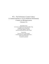
original graph as illustrated in Figure 1(a). These algorithms are often too slow and/or produce poor quality partitions. 

Multilevel partitioning algorithms, on the other hand, take a completely different approach [5, 8, 7]. These algorithms, 

as illustrated in Figure 1(b), reduce the size of the graph by collapsing vertices and edges, partition the smaller 

graph, and then uncoarsen it to construct a partition for the original graph. METIS uses novel approaches to successively 

reduce the size of the graph as well as to further refine the partition during the uncoarsening phase. During 

coarsening, METIS employs algorithms that make it easier to find a high-quality partition at the coarsest graph. During 

refinement, METIS focuses primarily on the portion of the graph that is close to the partition boundary. These highly 

tuned algorithms allow METIS to quickly produce high-quality partitions for a large variety of graphs. 

Traditional partitioning algorithms compute 

a partition directly on the original graph! 

(a) 

Multilevel partitioning algorithms compute a partition 

at the coarsest graph and then refine the solution! 

Coarsening Phase 

Initial Partitioning Phase 

(b) 

Refinement Phase 

Figure 1: (a) Traditional partitioning algorithms. (b) Multilevel partitioning algorithms. 

The advantages of METIS compared to other similar packages are the following: 

☞ Provides high quality partitions! 

Experiments on a large number of graphs arising in various domains including finite element methods, linear 

programming, VLSI, and transportation show that METIS produces partitions that are consistently better than 

those produced by other widely used algorithms. The partitions produced by METIS are consistently 10% to 

50% better than those produced by spectral partitioning algorithms [1, 4]. 

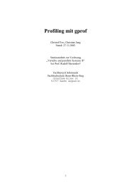
☞ It is extremely fast! 

Experiments on a wide range of graphs has shown that METIS is one to two orders of magnitude faster than other 

widely used partitioning algorithms. Figure 2 shows the amount of time required to partition a variety of graphs 

in 256 parts for two different architectures, an R10000-based SGI Challenge and a Pentium Pro-based personal 

computer. Graphs containing up to four million vertices can be partitioned in 256 parts in well under a minute 

on today’s scientific workstations. The run time of METIS is comparable to (or even smaller than) the run time 

of some geometric partitioning algorithms that often produce much worse partitions. 

☞ Provides low fill orderings! 

The fill-reducing orderings produced by METIS are substantially better than those produced by other widely 

used algorithms including multiple minimum degree. For many classes of problems arising in scientific computations 

and linear programming, METIS is able to reduce the storage and computational requirements of sparse 

matrix factorization methods by up to an order of magnitude. Moreover, unlike multiple minimum degree, the 

elimination trees produced by METIS are suited for parallel direct factorization. Furthermore, as Figure 2 illustrates, 

METIS is able to compute these ordering very fast. Matrices with over two hundred thousand rows can be 

reordered in just a few seconds on current generation workstations and PCs. 

4

Mdual3 

Big 

Mdual2 

Auto 

Troll 

Mdual1 

144 

Ocean 

Brack2 

Ocean 

Troll 

FORT17 

KEN18 

PDS-20 

BCSSTK31 

BCSSTK32 

BCSSTK30 

Inpro1 

METIS's Partitioning Performance 

4.42sec 

4.00sec 

3.79sec 

2.10sec 

2.55sec 

1.57sec 

7.79sec 

5.96sec 

5.87sec 

11.32sec 

17.81sec 

15.76sec 

16.95sec 

15.12sec 

19.40sec 

31.11sec 

47.34sec 

Number of 

Vertices 

Number of 

Edges 

Mdual3 4,039,160 8,016,848 

Big 295,433 7,953,453 

Mdual2 1,017,253 2,015,714 

Auto 448,695 3,314,611 

Troll 213,453 5,885,829 

Mdual1 257,000 505,048 

144 144,649 1,074,393 

Ocean 143,437 409,593 

Brack2 62,631 366,559 

MIPS R10000@200MHz Intel PPRO@200MHz 

METIS's Ordering Performance 

0.90sec 

2.67sec 

2.19sec 

1.52sec 

3.96sec 

3.55sec 

4.10sec 

3.43sec 

3.42sec 

3.95sec 

5.90sec 

6.55sec 

6.59sec 

10.51sec 

11.32sec 

13.34sec 

20.07sec 

24.43sec 

MIPS R10000@200MHz Intel PPRO@200MHz 

90.45sec 

Number of Number of Operation 

Vertices Edges Count 

Ocean 143,437 409,593 1.26e+08 

Troll 213,453 5,885,829 5.53e+10 

Fort17 86,650 247,424 8.05e+06 

Ken18 105,127 252,072 2.85e+08 

PDS-20 33,798 143,161 3.82e+09 

BCSSTK31 35,588 572,914 1.16e+09 

BCSSTK32 44,609 985,046 1.32e+09 

BCSSTK30 28,294 1,007,284 1.17e+09 

Inpro1 46,949 1,117,809 1.24e+09 

Figure 2: The amount of time required by METIS to partition various graphs in 256 parts and the amount of time required by METIS 

to compute fill-reducing orderings for various sparse matrices. 

The rest of this manual is organized as follows: Section 4 describes the user interface to the stand-alone programs 

provided by METIS. Section 5 describes the stand-alone library that implements the various algorithms implemented 

in METIS. Finally, Section 6 describes the system requirements for the METIS package. 

5

3 What is New in This Version 

The latest version of METIS contains a number of changes over the previous major release (version 3.0). Most of these 

changes are concentrated on the graph and mesh partitioning routines and they marginally affect the sparse matrix reordering 

routines. Table 1 describes which programs and routines of METISlib have been changed and the new routines 

in METISlib. In the rest of this section we briefly describe some of the major changes. 

Multi-Constraint Partitioning METIS now includes partitioning routines that can be used to partition a graph in 

the presence of multiple balancing constraints. The idea is that each vertex has a vector of weights of size m associated 

with it, and the objective of the partitioning algorithm is to minimize the edgecut subject to the constraints that each 

one of the m weights is equally distributed among the domains. For example, if the first weight corresponds to the 

amount of computation and the second weight corresponds to the amount of storage required for each element, then 

the partitioning computed by the new algorithms will balance both the computation performed in each domain as well 

as the amount of memory that it requires. Also, multi-phase (multi-physics) computations can use the new partitioning 

algorithm to simultaneously balance the computations performed in each phase. The multi-constraint partitioning 

algorithms and their applications are further described in [6]. 

The multi-constraint partitioning algorithm is implemented by the METIS mCPartGraphRecursive and 

METIS mCPartGraphKway routines that are based on the multilevel recursive bisection and the multilevel k-way 

partitioning paradigms, respectively. Also, the pmetis and the kmetis programs have been overloaded to invoke the 

multi-constraint partitioner when the input graph contains multiple vertex weights (Section 4.5.1 describes how the 

format of the input graph file has been extended to allow you to specify multiple vertex weights). 

Minimizing the Total Communication Volume The objective of the traditional graph partitioning problem is 

to compute a balanced k-way partitioning such that the number of edges (or in the case of weighted graphs the sum of 

their weights) that straddle different partitions is minimized. When partitioning is used to distribute a graph or a mesh 

among the processors of a parallel computer, the objective of minimizing the edgecut is only an approximation of the 

true communication cost resulting from the partitioning. Despite that, for a wide range of problems, by minimizing 

the edgecut, the partitioning algorithms also minimize the communication cost reasonably well. 

However, there are cases in which a partitioning algorithm can significantly reduce the communication cost by 

directly minimizing this objective (as opposed to the edgecut). METIS now provides the METIS PartGraphVKway 

and METIS WPartGraphVKway routines that directly minimize the communication cost as defined by the total 

communication volume resulted by the partitioning (see Section 5.3 for a precise definition of this objective function). 

Note that for these routines to provide meaningful partitionings, the connectivity of the graph should reflect the true 

information exchange requirements of the underlying computation. 

Minimizing the Maximum Connectivity of the Subdomains The communication cost resulting from a kway 

partitioning in general depends on the following factors: (i) the total communication volume, (ii) the maximum 

amount of data that any particular processor needs to send and receive; and (iii) the number of messages a processor 

needs to send and receive. The partitioning routines in earlier versions of METIS concentrated only on the first factor 

(by minimizing the edgecut). In this release, METIS also provides support for minimizing the third factor (which 

essentially reduces the number of startups) and indirectly (up to a point) reduces the second factor. Experiments have 

shown that for most graphs corresponding to finite element meshes, the new release of METIS is able to reduce the 

maximum (and total) number of adjacent subdomains considerably—especially when the graph is partitioned in a 

relatively large number of partitions (e.g., greater than 30). For most 3D finite elements graphs, the maximum number 

of subdomains for a 50-way partition has been reduced from around 25 to around 16. 

This enhancement is provided as a refinement option for both the METIS PartGraphKway and 

METIS PartGraphVKway routines, and is the default option of kmetis and METIS PartGraphKway. 

Reducing the Number of Non-Contiguous Subdomains A k-way partitioning of a contiguous graph can 

often lead to some subdomains being assigned non-contiguous portions of the graph. For many problems, the non- 

6

Changes in METIS’s stand-alone programs 

pmetis It has been over-loaded to invoke the multi-constraint partitioning algorithm 

when the graph contains multiple vertex weights. 

kmetis It has been over-loaded to invoke the multi-constraint partitioning algorithm 

when the graph contains multiple vertex weights. 

The partitioning algorithm has been modified to also minimize the connectivity 

of the subdomains. 

A pre- and post-refinement step is applied that tries to reduce the number 

of non-contiguous subdomains. 

partnmesh 

partdmesh 

Changes in METISlib’s routines 

METIS PartGraphKway 

METIS WPartGraphKway 

METIS PartGraphVKway 

METIS WPartGraphVKway 

METIS mCPartGraphRecursive 

METIS mCPartGraphKway 

The partitioning algorithm has been modified to also minimize the connectivity 

of the subdomains. 

A new refinement algorithm has been added that also minimizes the connectivity 

of the subdomains. This new algorithm has been made the default 

option. 

A pre- and post-refinement step is applied that tries to reduce the number 

of non-contiguous subdomains. 

This is a new set of routines that compute a k-way partitioning whose 

objective is to minimize the total communication volume. 

This is a new set of routines that compute a k-way partitioning subject to 

multiple balancing constraints. 

Table 1: Summary of the changes in METIS and METISlib. 

contiguity is a result of the underlying geometry and often leads to better quality partitions. Nevertheless, there are 

cases in which the partitioning algorithm is fooled and breaks certain domains. METIS now provides support for 

eliminating such spurious non-contiguous subdomains. 

This support is provided as a default option for both the METIS PartGraphKway and METIS PartGraphVKway 

routines, and the kmetis program. 

7

4 METIS’s Stand-Alone Programs 

METIS provides a variety of programs that can be used to partition graphs, partition meshes, compute fill-reducing 

orderings of sparse matrices, as well as programs to convert meshes into graphs appropriate for METIS’s graph partitioning 

programs. 

The rest of this section provides detailed descriptions about the functionality of these programs, how to use them, 

the format of the input files required by them, and the format of the produced output files. 

4.1 Graph Partitioning Programs 

METIS provides two programs pmetis and kmetis for partitioning an unstructured graph into k equal size parts. 

The partitioning algorithm used by pmetis is based on multilevel recursive bisection described in [8], whereas the 

partitioning algorithm used by kmetis is based on multilevel k-way partitioning described in [7]. Both of these 

programs are able to produce high quality partitions. However, depending on the application, one program may be 

preferable than the other. In general, kmetis is preferred when it is necessary to partition graphs into more than eight 

partitions. For such cases, kmetis is considerably faster than pmetis. On the other hand, pmetis is preferable 

for partitioning a graph into a small number of partitions. 

Both pmetis and kmetis are invoked by providing two arguments at the command line as follows: 

pmetis GraphFile Nparts 

kmetis GraphFile Nparts 

The first argument GraphFile, is the name of the file that stores the graph (whose format is described in Section 

4.5.1), while the second argument Nparts, is the number of partitions that is desired. Both pmetis and kmetis 

can partition a graph into an arbitrary number of partitions. Upon successful execution, both programs display statistics 

regarding the quality of the computed partitioning and the amount of time taken to perform the partitioning. The 

actual partitioning is stored in a file named GraphFile.part.Nparts, whose format is described in Section 4.6.1. 

Figure 3 shows the output of pmetis and kmetis for partitioning a graph into 100 parts. From this figure we 

see that both programs initially print information about the graph, such as its name, the number of vertices (#Vertices), 

the number of edges (#Edges), and also the number of desired partitions (#Parts). Next, they print some information 

regarding the quality of the partitioning. Specifically, they report the number of edges being cut (Edge-Cut) by the 

partitioning, as well as the balance of the partitioning 1 . Finally, both pmetis and kmetis show the time taken 

by the various phases of the algorithm. All times are in seconds. For this particular example, pmetis required a 

total of 17.070 seconds, of which 13.850 seconds was taken by the partitioning algorithm itself, and the rest was to 

read the graph itself. Similarly, kmetis required a total of 6.790 seconds, of which 3.570 seconds was taken by the 

partitioning algorithm itself. As you can see from this example, kmetis is considerably faster than pmetis, and it 

produces a partitioning that is slightly better than that produced by pmetis. 

Figure 4 shows the output of pmetis and kmetis for partitioning a graph into 16 parts subject to three balancing 

constraints. Both pmetis and kmetis have been over-loaded to invoke the multi-constraint partitioning routines 

whenever the input graph file specifies more that one set of vertex weights. Comparing the output of Figure 4 to that 

of Figure 3 we see that when pmetis and kmetis operate in the multi-constraint mode they display some additional 

information regarding the number of constraints and also the balance of the computed partitioning with respect to each 

one of these constraints. In this example, pmetis was able to balance the three constraints within 1%, 3%, and 2%, 

respectively. Note that for multi-constraint partitioning, for small number of partitions pmetis outperforms kmetis 

in terms of partitioning quality. However, for larger number of partitions kmetis achieves better quality and is more 

robust in simultaneously balancing the various constraints. 

1 For a k way partition of a graph with n vertices, let m be the size of the largest part produced by the k-way partitioning algorithm. The balance 

of the partitioning is defined as km/n, and is essentially the load imbalance induced by non-equal partitions. pmetis produces partitions that are 

perfectly balanced at each bisection level, however, some small load imbalance may result due to the log k levels of recursive bisection. In general, 

the load imbalance is less than 1%. kmetis produces partitions that are not perfectly balanced, but the algorithm limits the load imbalance to 3%. 

8

' 

prompt% pmetis brack2.graph 100 

********************************************************************** 

METIS 4.0 Copyright 1998, Regents of the University of Minnesota 

Graph Information --------------------------------------------------- 

Name: brack2.graph, #Vertices: 62631, #Edges: 366559, #Parts: 100 

Recursive Partitioning... ------------------------------------------- 

100-way Edge-Cut: 37494, Balance: 1.00 

Timing Information -------------------------------------------------- 

I/O: 0.820 

Partitioning: 6.110 (PMETIS time) 

Total: 6.940 

********************************************************************** 

prompt% kmetis brack2.graph 100 

********************************************************************** 



Name: brack2.graph, #Vertices: 62631, #Edges: 366559, #Parts: 100 

K-way Partitioning... ----------------------------------------------- 



I/O: 0.820 

Partitioning: 1.750 (KMETIS time) 

Total: 2.570 

********************************************************************** 

& 

Figure 3: Output of pmetis and kmetis for graph brack2.graph and a 100-way partition. 

4.2 Mesh Partitioning Programs 

$ 

% 

METIS provides two programs partnmesh and partdmesh for partitioning meshes (e.g., those arising in finite 

element or finite volume methods) into k equal size parts. These programs take as input the element node array of the 

mesh and compute a partitioning for both its elements and its nodes. METIS currently supports four different types of 

mesh elements which are triangles, tetrahedra, hexahedra (bricks), and quadrilaterals. 

These programs first convert the mesh into a graph, and then use kmetis to partition this graph. The difference 

between these two programs is that partnmesh converts the mesh into a nodal graph (i.e., each node of the mesh 

becomes a vertex of the graph), whereas partdmesh converts the mesh into a dual graph (i.e., each element becomes 

a vertex of the graph). In the case of partnmesh, the partitioning of the nodal graph is used to derive a partitioning of 

the elements. In the case of partdmesh, the partitioning of the dual graph is used to derive a partitioning of the nodes. 

Both of these programs produce partitioning of comparable quality, with partnmesh being considerably faster than 

partdmesh. However, in some cases, partnmesh may produce partitions that have higher load imbalance than 

partdmesh. 

Both partnmesh and partdmesh are invoked by providing two arguments at the command line as follows: 

partnmesh MeshFile Nparts 

partdmesh MeshFile Nparts 

The first argument MeshFile, is the name of the file that stores the mesh (whose format is described in Section 4.5.2), 

while the second argument Nparts, is the number of partitions that is desired. Both partnmesh and partdmesh can 

partition a mesh into an arbitrary number of partitions. Upon successful execution, both programs display statistics 

regarding the quality of the computed partitioning and the amount of time taken to perform the partitioning. The 

9

' 

prompt% pmetis m14.graph3 16 

********************************************************************** 



Name: m14.graph3, #Vertices: 214765, #Edges: 1679018, #Parts: 16 

Balancing Constraints: 3 

Recursive Partitioning... ------------------------------------------- 

16-way Edge-Cut: 74454, Balance: 1.01 1.03 1.02 


I/O: 4.310 

Partitioning: 28.410 (PMETIS time) 

Total: 32.830 

********************************************************************** 

prompt% kmetis m14.graph3 16 

********************************************************************** 



Name: m14.graph3, #Vertices: 214765, #Edges: 1679018, #Parts: 16 

Balancing Constraints: 3 

K-way Partitioning... ----------------------------------------------- 

16-way Edge-Cut: 71410, Balance: 1.04 1.04 1.04 


I/O: 4.020 

Partitioning: 7.430 (KMETIS time) 

Total: 11.550 

********************************************************************** 

& 

$ 

% 

Figure 4: Output of pmetis and kmetis for a multi-constraint graph with three constraints and a 16-way partition. 

actual partitioning is stored in two files named: MeshFile.npart.Nparts which stores the partitioning of the nodes, and 

MeshFile.epart.Nparts which stores the partitioning of the elements. The format of the partitioning files is described 

in Section 4.6.1. 

Figure 5 shows the output of partnmesh and partdmesh for partitioning a mesh with tetrahedron elements into 

100 parts. From this figure we see that both programs initially print information about the mesh, such as its name, the 

number of elements (#Elements), the number of nodes (#Nodes), and the type of elements (e.g., TET). Next, they print 

some information regarding the quality of the partitioning. Specifically, they report the number of edges being cut 

(Edge-Cut) by the partitioning 2 , as well as the balance of the partitioning. For both partnmesh and partdmesh, 

the balance is computed with respect to the number of elements. The balance with respect to the number of nodes is 

not shown, but it is in general similar to the element balance. 

Finally, both partnmesh and partdmesh show the time that was taken by the various phases of the algorithm. 

All times are in seconds. In this particular example, it took partnmesh 23.370 seconds to partition the mesh into 

100 parts. Note that this time includes the time required both to construct the nodal graph and to partition it. Similarly, 

it took partdmesh 74.560 seconds to partition the same mesh. Again, this time includes the time required both to 

construct the dual graph and to partition it. As you can see from this example, partnmesh is considerably faster 

than partdmesh. This is because of two reasons: (i) the time required to construct the nodal graph is smaller than 

the time required to construct the dual graph; (ii) the nodal graph is smaller than the dual graph. 

2 The edgecut that is reported by partnmesh is that of the nodal graph, whereas the edgecut reported by partdmesh is that of the dual graph. 

These two edgecuts cannot be compared with each other, as they correspond to partitionings of two totally different graphs. 

10

Note If you need to compute multiple partitionings of the same mesh, it may be preferable to first use one of 

the mesh conversion programs described in Section 4.4 to first convert the mesh into a graph, and then use 

kmetis to partition it. By doing this, you pay the cost of converting the mesh into a graph only once. 

' 

prompt% partnmesh 144.mesh 100 

********************************************************************** 


Mesh Information ---------------------------------------------------- 

Name: 144.mesh, #Elements: 905410, #Nodes: 144649, Etype: TET 

Partitioning Nodal Graph... ----------------------------------------- 



I/O: 13.210 

Partitioning: 7.950 

********************************************************************** 

prompt% partdmesh 144.mesh 100 

********************************************************************** 




Partitioning Dual Graph... ------------------------------------------ 



I/O: 11.540 

Partitioning: 28.220 

********************************************************************** 

& 

Figure 5: Output of partnmesh and partdmesh for mesh 144.mesh and a 100-way partition. 

4.3 Sparse Matrix Reordering Programs 

$ 

% 

METIS provides two programs oemetis and onmetis for computing fill-reducing orderings of sparse matrices. 

Both of these programs use multilevel nested dissection to compute a fill-reducing ordering [8]. The nested dissection 

paradigm is based on computing a vertex-separator for the the graph corresponding to the matrix. The nodes in the 

separator are moved to the end of the matrix, and a similar process is applied recursively for each one of the other two 

parts. 

Even though both programs are based on multilevel nested dissection, they differ on how they compute the vertex 

separators. The oemetis program finds a vertex separator by first computing an edge separator using a multilevel 

algorithm, whereas the onmetis program uses the multilevel paradigm to directly find a vertex separator. The orderings 

produced by onmetis generally incur less fill than those produced by oemetis. In particular, for matrices 

arising in linear programming problems the orderings computed by onmetis are significantly better than those produced 

by oemetis. Furthermore, onmetis utilizes compression techniques to reduce the size of the graph prior to 

computing the ordering. Sparse matrices arising in many application domains are such that certain rows of the matrix 

have the same sparsity pattern. Such matrices can be represented by a much smaller graph in which all rows with 

identical sparsity pattern are represented by just a single vertex whose weight is equal to the number of rows. Such 

compression techniques can significantly reduce the size of the graph, whenever applicable, and substantially reduce 

the amount of time required by onmetis. However, when there is no reduction in graph size, oemetis is about 

20% to 30% faster than onmetis. Furthermore, for large matrices arising in three-dimensional problems, the quality 

11

' 

prompt% oemetis bcsstk31.graph 

********************************************************************** 



Name: bcsstk31.graph, #Vertices: 35588, #Edges: 572914 

Edge-Based Ordering... ---------------------------------------------- 

Nonzeros: 4693428, Operation Count: 1.4356e+09 


I/O: 1.160 

Ordering: 7.380 (OEMETIS time) 

Symbolic Factorization: 0.440 

Total: 8.980 

********************************************************************** 

prompt% onmetis bcsstk31.graph 

********************************************************************** 



Name: bcsstk31.graph, #Vertices: 35588, #Edges: 572914 

Node-Based Ordering... ---------------------------------------------- 

Nonzeros: 4330669, Operation Count: 1.1564e+09 


I/O: 1.080 

Ordering: 4.540 (ONMETIS time) 

Symbolic Factorization: 0.440 

Total: 6.060 

********************************************************************** 

& 

Figure 6: Output of oemetis and onmetis for graph bcsstk31.graph. 

of orderings produced by the two algorithms is quite similar. 

Both oemetis and onmetis are invoked by providing one argument at the command line as follows: 

oemetis GraphFile 

onmetis GraphFile 

$ 

% 

The only argument of these programs GraphFile, is the name of the file that stores the sparse matrix in the graph 

format described in Section 4.5.1. Upon successful execution, both programs display statistics regarding the quality 

of the computed orderings and the amount of time taken to perform the ordering. The actual ordering is stored in a file 

named GraphFile.iperm, whose format is described in Section 4.6.2. 

Figure 6 shows the output of oemetis and onmetis for computing a fill-reducing ordering of a sample matrix. 

From this figure we see that both programs initially print information about the graph, such as its name, the number 

of vertices (#Vertices), and the number of edges (#Edges). Next, they print some information regarding the quality of 

the ordering. Specifically, they report the number of non-zeros that are required in the lower triangular matrix, and the 

number of operations (OPC) required to factor the matrix using Cholesky factorization. Note that number of nonzeros 

includes both the original non-zeros and the new non-zeros due to the fill. Finally, both oemetis and onmetis 

show the time that was taken by the various phases of the algorithm. All times are in seconds. For this particular 

example, oemetis takes a total of 23.290 seconds, of which 17.760 seconds was taken by the ordering algorithm 

itself. For the same example onmetis takes a total of 17.340 seconds, of which 11.810 seconds was taken by the 

partitioning algorithm itself. Note that in this case onmetis is faster than oemetis, because onmetis was able 

to compress the matrix. Also note that the quality of the fill-reducing ordering produced by onmetis is significantly 

better than that produced by oemetis. In fact, the ordering produced by onmetis results in 8% fewer non-zeros 

12

and 20% fewer operations. 

4.4 Auxiliary Programs 

4.4.1 Mesh To Graph Conversion 

' 

prompt% mesh2nodal 144.mesh 

********************************************************************** 




Forming Nodal Graph... ---------------------------------------------- 

Nodal Information: #Vertices: 144649, #Edges: 1074393 


I/O: 15.290 

Nodal Creation: 3.030 

********************************************************************** 

prompt% mesh2dual 144.mesh 

********************************************************************** 




Forming Dual Graph... ----------------------------------------------- 

Dual Information: #Vertices: 905410, #Edges: 1786484 


I/O: 19.200 

Dual Creation: 10.880 

********************************************************************** 

& 

Figure 7: Output of mesh2nodal and mesh2dual for mesh 144.mesh. 

$ 

% 

METIS provides two programs mesh2nodal and mesh2dual for converting a mesh into the graph format used 

by METIS. In particular, mesh2nodal converts the element node array of a mesh into a nodal graph; i.e., each node 

of the mesh corresponds to a vertex in the graph and two vertices are connected by an edge if the corresponding 

nodes are connected by lines in the mesh. Similarly, mesh2dual converts the element node array of a mesh into 

a dual graph; i.e., each element of the mesh corresponds to a vertex in the graph and two vertices are connected if 

the corresponding elements in the mesh share a face. These mesh-to-graph conversion programs support meshes with 

triangular, tetrahedra, and hexahedra (bricks) elements. 

Both mesh2nodal and mesh2dual are invoked by providing one argument at the command line as follows: 

mesh2nodal MeshFile 

mesh2dual MeshFile 

The only argument of these programs MeshFile, is the name of the file that stores the mesh (whose format is 

described in Section 4.5.2). Upon successful execution, both programs display information about the generated graphs, 

and the amount of time taken to perform the conversion. The actual graph is stored in a file named: MeshFile.ngraph 

in the case of mesh2nodal and MeshFile.dgraph in the case of mesh2dual. The format of these graph files are 

compatible with METIS and is described in Section 4.5.1. 

Figure 7 shows the output of mesh2nodal and mesh2dual for generating the nodal and dual graphs of a sample 

mesh. Note that the sizes of the generated graphs are different, as the dual graph is larger than the nodal graph. Also 

note that generating the nodal graph is considerably faster than generating the dual graph. 

13

4.4.2 Graph Checker 

METIS provide a program called graphchk to check whether or not the format of a graph is appropriate for use with 

METIS. This program should be used whenever there is any doubt about the format of any graph file. It is invoked by 

providing one argument at the command line as follows: 

graphchk GraphFile 

where GraphFile is the name of the file that stores the graph. 

14

4.5 Input File Formats 

The various programs in METIS require as input either a file storing a graph or a file storing a mesh. The format of 

these files are described in the following sections. 

4.5.1 Graph File 

The primary input of the partitioning and fill-reducing ordering programs in METIS is the graph to be partitioned or 

ordered. This graph is stored in a file and is supplied to the various programs as one of the command line parameters. 

A graph G = (V, E) with n vertices and m edges is stored in a plain text file that contains n + 1 lines (excluding 

comment lines). The first line contains information about the size and the type of the graph, while the remaining n 

lines contain information for each vertex of G. Any line that starts with ‘%’ is a comment line and is skipped. 

The first line contains either two (n, m), three (n, m, fmt), or four (n, m, fmt, ncon) integers. The first two integers 

(n, m) are the number of vertices and the number of edges, respectively. Note that in determining the number of edges 

m, an edge between any pair of vertices v and u is counted only once and not twice (i.e., we do not count the edge 

(v, u) separately from (u,v)). For example, the graph in Figure 8 contains 11 vertices. The third integer (fmt) is used 

to specify whether or not the graph has weights associated with its vertices, its edges, or both. Table 2 describes the 

possible values of fmt and their meaning. Note that if the graph is unweighted (i.e., all vertices and edges have the 

same weight), then the fmt parameter can be omitted. Finally, the fourth integer (ncon) is used to specify the number 

of weights associated with each vertex of the graph. The value of this parameter determines whether or not METIS will 

use the multi-constraint partitioning algorithms described in Section 3. If the vertices of the graph have no weights or 

only a single weight, then the ncon parameter can be omitted. However, if ncon is greater than 0, then the file should 

contain the required vertex weights and the fmt parameter should be set appropriately (i.e., it should be set to either 10 

or 11). 

fmt Meaning 

0 The graph has no weights associated with either the edges or the vertices 

1 The graph has weights associated with the edges 

10 The graph has weights associated with the vertices 

11 The graph has weights associated with both the edges & vertices 

Table 2: The various possible values for the fmt parameter and their meaning. 

The remaining n lines store information about the actual structure of the graph. In particular, the ith line (excluding 

comment lines) contains information that is relevant to the ith vertex. Depending on the value of the fmt and ncon 

parameters, the information stored at each line is somewhat different. In the most general form (when fmt = 11 and 

ncon > 1) each line will have the following structure: 

w1,w2,...wncon, v1, e1,v2, e2,...,vk, ek 

where w1,w2,...,wncon are the ncon vertex weights associated with this vertex, v1,v2,...,vk are the vertices adjacent 

to this vertex, and e1, e2,...,ek are the weights of these edges. In the remaining of this section we illustrate this 

format by a sequence of examples. Note that the vertices are numbered starting from 1 (not from 0 as is often done in 

C). Furthermore, the vertex-weights must be integers greater or equal to 0, whereas the edge-weights must be strictly 

greater than 0. 

The simplest format for a graph G is when the weight of all vertices and the weight of all the edges is the same. 

This format is illustrated in Figure 8(a). Note, the optional fmt parameter is skipped in this case. 

However, there are cases in which the edges in G have different weights. This is accommodated as shown in 

Figure 8(b). Now, the adjacency list of each vertex contains the weight of the edges in addition to the vertices that is 

connected with. If v has k vertices adjacent to it, then the line for v in the graph file contains 2 ∗ k numbers, each pair 

of numbers stores the vertex that v is connected to, and the weight of the edge. Note that the fmt parameter is equal 

15

2 

1 

Graph File: 

[4] 

1 

1 

[2] 

2 

5 

3 

7 11 

5 3 2 

1 3 4 

5 4 2 1 

2 3 6 7 

1 3 6 

5 4 7 

6 4 

1 

Graph File: 

4 

6 

(a) Unweighted Graph 

2 

2 

[1] 

5 

[5] 

3 

2 

1 

3 

4 

[3] 

[6] 

6 

7 11 11 

4 5 1 3 2 2 1 

2 1 1 3 2 4 1 

5 5 3 4 2 2 2 1 2 

3 2 1 3 2 6 2 7 5 

1 1 1 3 3 6 2 

6 5 2 4 2 7 6 

2 6 6 4 5 

(c) Weighted Graph 

Weights both on vertices and edges 

2 

2 

5 

6 

7 

7 

[2] 

1 

2 

1 

2 

1 

1 

Graph File: 

[0, 2, 2] 

[1, 2, 0] 

2 

2 

5 

1 

3 

3 

5 

2 

2 

4 

2 

7 11 1 

5 1 3 2 2 1 

1 1 3 2 4 1 

5 3 4 2 2 2 1 2 

2 1 3 2 6 2 7 5 

1 1 3 3 6 2 

5 2 4 2 7 6 

6 6 4 5 

Graph File: 

[4, 1, 1] 

3 

7 11 10 3 

1 2 0 5 3 2 

0 2 2 1 3 4 

4 1 1 5 4 2 1 

2 2 3 2 3 6 7 

1 1 1 1 3 6 

2 2 1 5 4 7 

1 2 1 6 4 

6 

(b) Weighted Graph 

Weights on edges 

[1, 1, 1] 

Figure 8: Storage format for various type of graphs. 

5 

[2, 2, 1] 

6 

4 

[2, 2, 3] 

(d) Multi-Constraint Graph 

to 1, indicating the fact that G has weights on the edges. 

In addition to having weights on the edges, weights on the vertices are also allowed, as illustrated in Figure 8(c). In 

this case, the value of fmt is equal to 11, and each line of the graph file first stores the weight of the vertex, and then 

the weighted adjacency list. 

Finally, Figure 8(d) illustrates the format of the input file when the vertices of the graph contain multiple weights 

(3 in this example). In this case, the value of fmt is equal to 10 (we do not have weights associated with the edges), 

and the value of ncon is equal to 3 (since we have three sets of vertex-weights). Each line of the graph file stores the 

three weights of the vertices followed by the adjacency list. 

4.5.2 Mesh File 

The primary input of the mesh partitioning programs in METIS is the mesh to be partitioned. This mesh is stored in 

a file in the form of the element node array. A mesh with n elements is stored in a plain text file that contains n + 1 

16 

6 

7 

[1, 2, 1] 

7

lines. The first line contains information about the size and the type of the mesh, while the remaining n lines contain 

the nodes that make up each element. 

The first line contains two integers. The first integer is the number of elements n in the mesh. The second integer 

etype is used to denote the type of elements that the mesh is made off. Etype can either take the values of 1, 2, 3, or 4, 

indicating that the mesh consists of either triangles, tetrahedra, hexahedra (bricks), or quadrilaterals, respectively. 

After the first line, the remaining n lines store the element node array. In particular for element i, line i + 1 stores 

the nodes that this element is made off. Depending on etype, each line can either have three integers (in the case of 

triangles), four integers (in the case of tetrahedra and quadrilaterals), or eight integers (in the case of hexahedra). In 

the case of triangles and tetrahedra, the ordering of the nodes for each element does not matter. However, in the case 

of hexahedra and quadrilaterals, the nodes for each element should be ordered according to the numbering illustrated 

in Figure 9(b). Note that the node numbering starts from 1. 

Figure 9 illustrates this format for a small mesh with triangular elements. Note that the etype field of the mesh file 

is set to 1 indicating that the mesh consists of triangular elements. 

4 

2 

Mesh File: 

6 

1 

(a) Sample Mesh File 

5 

3 

5 1 

1 2 3 

2 4 6 

2 6 3 

4 5 6 

5 6 3 

6 

2 

5 

1 

7 

3 

8 

4 

(b) Ordering of nodes 

Figure 9: (a) The file that stores the mesh. (b) The ordering of the nodes in the case of hexahedra and quadrilaterals. 

4.6 Output File Formats 

The output of METIS is either a partition or an ordering file, depending on whether METIS is used for graph/mesh 

partitioning or for sparse matrix ordering. The format of these files are described in the following sections. 

4.6.1 Partition File 

The partition file of a graph with n vertices consists of n lines with a single number per line. The ith line of the 

file contains the partition number that the ith vertex belongs to. Partition numbers start from 0 up to the number of 

partitions minus one. 

4.6.2 Ordering File 

The ordering file of a graph with n vertices consists of n lines with a single number per line. The ith line of the 

ordering file contains the new order of the ith vertex of the graph. The numbering in the ordering file starts from 0. 

Note that the ordering file stores what is referred to as the the inverse permutation vector iperm of the ordering. Let 

A be a matrix and let A ′ be the reordered matrix. The inverse permutation vector maps the ith row (column) of A into 

the iperm[i] row (column) of A ′ . 

17 

2 

1 

3 

4

5 METIS’s Library Interface 

The various programs provided in METIS can also be directly accessed from a C or Fortran program by using the standalone 

library METISlib. Furthermore, METISlib extends the functionality provided by METIS’s stand-alone programs 

in two different ways. First, it allows the user to alter the behavior of the various algorithms in METIS, and second 

METISlib provides additional routines that can be used to partition graphs into unequal-size partitions and compute 

partitionings that directly minimize the total communication volume. 

In the rest of this section we describe the interface to the routines in METISlib by first describing the various data 

structures used to pass information into and get information out of the routines, followed by a detailed description of 

the calling sequence of the various routines. 

5.1 Graph Data Structure 

All of the graph partitioning and sparse matrix ordering routines in METISlib take as input the adjacency structure of 

the graph and the weights of the vertices and edges (if any). 

The adjacency structure of the graph is stored using the compressed storage format (CSR). The CSR format is a 

widely used scheme for storing sparse graphs. In this format the adjacency structure of a graph with n vertices and 

m edges is represented using two arrays xadj and adjncy. The xadj array is of size n + 1 whereas the adjncy 

array is of size 2m (this is because for each edge between vertices v and u we actually store both (v, u) and (u,v)). 

The adjacency structure of the graph is stored as follows. Assuming that vertex numbering starts from 0 (C style), 

then the adjacency list of vertex i is stored in array adjncy starting at index xadj[i] and ending at (but not 

including) index xadj[i + 1] (i.e., adjncy[xadj[i]] through and including adjncy[xadj[i + 1]-1]). That 

is, for each vertex i, its adjacency list is stored in consecutive locations in the array adjncy, and the array xadj is 

used to point to where it begins and where it ends. Figure 10(b) illustrates the CSR format for the 15-vertex graph 

shown in Figure 10(a). 

xadj 

adjncy 

0 1 2 3 4 

5 

10 

6 

11 

7 

12 

13 

14 

(a) A sample graph 

0 2 5 8 11 13 16 20 24 28 31 33 36 39 42 44 

8 

9 

1 5 0 2 6 1 3 7 2 4 8 3 9 0 6 10 1 5 7 11 2 6 8 12 3 7 9 13 4 8 14 5 11 6 10 12 7 11 13 8 12 14 9 13 

(b CSR format 

Figure 10: An example of the CSR format for storing sparse graphs. 

The weights of the vertices (if any) are stored in an additional array called vwgt. Ifncon is the number of weights 

associated with each vertex, the array vwgt contains n ∗ ncon elements (recall that n is the number of vertices). The 

weights of the ith vertex are stored in ncon consecutive entries starting at location vwgt[i ∗ ncon]. Note that if 

each vertex has only a single weight, then vwgt will contain n elements, and vwgt[i] will store the weight of the 

ith vertex. The vertex-weights must be integers greater or equal to zero. If all the vertices of the graph have the same 

weight (i.e., the graph is unweighted), then the vwgt can be set to NULL. 

The weights of the edges (if any) are stored in an additional array called adjwgt. This array contains 2m elements, 

and the weight of edge adjncy[ j] is stored at location adjwgt[ j]. The edge-weights must be integers greater 

than zero. If all the edges of the graph have the same weight (i.e., the graph is unweighted), then the adjwgt can be 

set to NULL. 

All of these four arrays (xadj, adjncy, vwgt, and adjwgt) are defined in METISlib to be of of type idxtype. By 

default idxtype is set to be equivalent to type int (i.e., the integer datatype of C). However, idxtype can be 

18

made to be equivalent to a short int for certain architectures that use 64-bit integers by default. The conversion of 

idxtype from int to short can be done by modifying the file Lib/struct.h (instructions are included there). 

The same idxtype is used for the arrays that are used to store the computed partition and permutation vector. 

5.2 Mesh Data Structure 

All of the mesh partitioning and mesh conversion routines in METISlib take as input the element node array of a mesh. 

This element node array is stored using an array called elmnts. For a mesh with n elements and k nodes per element, 

the size of the elmnts array is n ∗ k. Note that since the supported elements in METIS are only triangles, tetrahedra, 

hexahedra, and quadrilaterals, the possible values for k are 3, 4, 8, and 4, respectively. 

The element node array of the mesh is stored in elmnts as follows. Assuming that the element numbering starts 

from 0 (C style), then the k nodes that make up element i are stored in array elmnts starting at index i ∗ k and ending 

(but not including) index (i + 1) ∗ k. As it was the case with the format of the mesh file described in Section 4.5.2, 

the ordering of the nodes is not important for triangle and tetrahedra elements. However, in the case of hexahedra, the 

nodes for each element must be ordered according to the numbering illustrated in Figure 9(b). 

The array that describes the element node array of the mesh is defined in METISlib to be of type idxtype, which 

by default is equivalent to int (i.e., integers). 

5.3 Partitioning Objectives 

The partitioning algorithms in METISlib can be used to compute a balanced k-way partitioning that minimizes either 

the number of edges that straddle partitions (edgecut) or the total communication volume (totalv). In the rest of this 

section we briefly describe these two objectives and provide some suggestions on when they should be used. 

Minimizing the Edge-Cut Consider a graph G = (V, E), and let P be a vector of size |V | such that P[i] stores 

the number of the partition that vertex i belongs to. The edgecut of this partitioning is defined as the number of edges 

that straddle partitions. That is, the number of edges (v, u) for which P[v] =P[u]. If the graph has weights associated 

with the edges, then the edgecut is defined as the sum of the weight of these straddling edges. 

Minimizing the Total Communication Volume Consider a graph G = (V, E), and let P be a vector of size 

|V | such that P[i] stores the number of the partition that vertex i belongs to. Let Vb ⊂ V be the subset of interface (or 

boarder) vertices. That is, each vertex v ∈ Vb is connected to at least one vertex that belongs to a different partition. 

For each vertex v ∈ Vb let Nadj[v] be the number of domains other than P[v] that the vertices adjacent to v belong 

to. The totalv of this partitioning is defined as: 

totalv = 

Nadj[v]. (1) 

v∈Vb 

Equation 1 corresponds to the total communication volume incurred by the partitioning because each interface vertex 

v needs to be sent to all of its Nadj[v] partitions. 

The above model can be extended to instances in which the amount of data that needs to be sent for each node is 

different. In particular, if wv is the amount of data that needs to be sent for vertex v, then Equation 1 can be re-written 

as: 

totalv = 

wv Nadj[v]. (2) 

v∈Vb 

METISlib supports this weighted totalv model by using an array called vsize such that the amount of data that needs 

to be sent due to the ith vertex is stored in vsize[i]. Note that the amount of data that needs to be sent is different 

from the weight of the vertex. The former corresponds to communication cost whereas the later corresponds to the 

computational cost. 

Note that for partitioning algorithms to correctly minimize the totalv, the graph should reflect the true information 

exchange requirements of the underlying computations. For instance, the dual graph of a finite element mesh does not 

19

correctly model the underlying communication, whereas the nodal graph does. 

Which one is Better? When partitioning is used to distribute a graph or a mesh among the processors of a parallel 

computer, the edgecut is only an approximation of the true communication cost resulting from the partitioning. On 

the other hand, by minimizing the totalv we can directly minimize the overall communication cost. Despite of that, 

for many graphs the solutions obtained by minimizing the edgecut or minimizing the totalv, are comparable. This 

is especially true for graphs corresponding to well-shaped finite element meshes. This is because for these graphs, 

the degrees of the various vertices are similar and the objectives of minimizing the edgecut or the totalv behave the 

same. On the other hand, if the vertex degrees vary significantly (e.g., graphs corresponding to linear programming 

matrices), then by minimizing the totalv we can obtain a significant reduction in the total communication volume. 

In terms of the amount of time required by these two partitioning objectives, minimizing the edgecut is faster than 

minimizing the totalv. For this reason, the totalv objective should be used only for problems in which it actually 

reduces the overall communication volume. 

20

5.4 Graph Partitioning Routines 

METIS PartGraphRecursive (int *n, idxtype *xadj, idxtype *adjncy, idxtype *vwgt, idxtype *adjwgt, int *wgtflag, 

int *numflag, int *nparts, int *options, int *edgecut, idxtype *part) 

Description 

It is used to partition a graph into k equal-size parts using multilevel recursive bisection. It provides the functionality 

of the pmetis program. The objective of the partitioning is to minimize the edgecut (as described in 

Section 5.3). 

Parameters 

n The number of vertices in the graph. 

xadj, adjncy 

The adjacency structure of the graph as described in Section 5.1. 

vwgt, adjwgt 

Information about the weights of the vertices and edges as described in Section 5.1. 

wgtflag Used to indicate if the graph is weighted. wgtflag can take the following values: 

0 No weights (vwgts and adjwgt are NULL) 

1 Weights on the edges only (vwgts = NULL) 

2 Weights on the vertices only (adjwgt = NULL) 

3 Weights both on vertices and edges. 

numflag Used to indicate which numbering scheme is used for the adjacency structure of the graph. numflag 

can take the following two values: 

0 C-style numbering is assumed that starts from 0 

1 Fortran-style numbering is assumed that starts from 1 

nparts The number of parts to partition the graph. 

options This is an array of 5 integers that is used to pass parameters for the various phases of the algorithm. 

If options[0]=0 then default values are used. If options[0]=1, then the remaining four elements of 

options are interpreted as follows: 

options[1] Determines matching type. Possible values are: 

1 Random Matching (RM) 

2 Heavy-Edge Matching (HEM) 

3 Sorted Heavy-Edge Matching (SHEM) (Default) 

Experiments has shown that both HEM and SHEM perform quite well. 

options[2] Determines the algorithm used during initial partitioning. Possible values are: 

1 Region Growing (Default) 

options[3] Determines the algorithm used for refinement. Possible values are: 

1 Early-Exit Boundary FM refinement (Default) 

options[4] Used for debugging purposes. Always set it to 0 (Default). 

edgecut Upon successful completion, this variable stores the number of edges that are cut by the partition. 

part This is a vector of size n that upon successful completion stores the partition vector of the graph. The 

numbering of this vector starts from either 0 or 1, depending on the value of numflag. 

Note 

This function should be used to partition a graph into a small number of partitions (less than 8). If a large number 

of partitions is desired, the METIS PartGraphKway should be used instead, as it is significantly faster. 

21

METIS PartGraphKway (int *n, idxtype *xadj, idxtype *adjncy, idxtype *vwgt, idxtype *adjwgt, int *wgtflag, 

int *numflag, int *nparts, int *options, int *edgecut, idxtype *part) 

Description 

It is used to partition a graph into k equal-size parts using the multilevel k-way partitioning algorithm. It 

provides the functionality of the kmetis program. The objective of the partitioning is to minimize the edgecut 

(as described in Section 5.3). 

Parameters 


xadj, adjncy 


vwgt, adjwgt 















options[1] Determines the matching type. Possible values are: 






1 Multilevel recursive bisection (Default) 


1 Random boundary refinement 

2 Greedy boundary refinement 

3 Random boundary refinement that also minimizes the connectivity among the subdomains 

(Default) 





Note 

This function should be used to partition a graph into a large number of partitions (greater than 8). If a small 

number of partitions is desired, the METIS PartGraphRecursive should be used instead, as it produces somewhat 

better partitions. 

22

METIS PartGraphVKway (int *n, idxtype *xadj, idxtype *adjncy, idxtype *vwgt, idxtype *vsize, int *wgtflag, 

int *numflag, int *nparts, int *options, int *volume, idxtype *part) 

Description 

It is used to partition a graph into k equal-size parts using the multilevel k-way partitioning algorithm. The 

objective of the partitioning is to minimize the total communication volume (as described in Section 5.3). 

Parameters 


xadj, adjncy 

The adjacency structure of the graph as described in Sections 5.1 and 5.3. 

vwgt, vsize 

Information about the weights of the vertices related to the computation and communication as described 

in Section 5.1. 


0 No weights (vwgts and vsize are NULL) 

1 Communication weights only (vwgts = NULL) 

2 Computation weights only (vsize = NULL) 

3 Both communication and computation weights. 

















1 Random boundary refinement (Default) 



volume Upon successful completion, this variable stores the total communication volume requires by the 

partition. 



23

METIS mCPartGraphRecursive (int *n, int *ncon, idxtype *xadj, idxtype *adjncy, idxtype *vwgt, idxtype *adjwgt, 

int *wgtflag, int *numflag, int *nparts, int *options, int *edgecut, idxtype *part) 

Description 

It is used to partition a graph into k parts such that multiple balancing constraints are satisfied. It uses the multiconstraint 

multilevel recursive bisection algorithm. It provides the functionality of the pmetis program when 

it is used to compute a multi-constraint partitioning. The objective of the partitioning is to minimize the edgecut 


Parameters 


ncon The number of constraints. This should be greater than one and smaller than 15. 

xadj, adjncy 


vwgt, adjwgt 

Information about the weights of the vertices and edges as described in Section 5.1. Note that the 

weight vector must be supplied and it should be of size n*ncon. 


0 No weights (adjwgt is NULL) 

1 Weights on the edges. 













5 Sorted Heavy-Edge Matching followed by 1-norm Balanced-edge (SHEBM1N) 

6 Sorted Heavy-Edge Matching followed by ∞-norm Balanced-edge (SHEBMIN) 

(Default) 

7 1-norm Balanced-edge followed by Heavy-Edge Matching (SBHEM1N) 

8 ∞-norm Balanced-edge followed by Heavy-Edge Matching (SBHEMIN) 

Experiments has shown that for simple balancing problems, the schemes that give priority 

to heavy edges (e.g., SHEM, SHEBM1N, SHEBMIN) perform better, and for hard 

balancing problems, the schemes that give priority to balanced edges (e.g., SBHEM1N, 

SBHEMIN) perform better. 


1 Multi-constraint Greedy Graph Growing 

2 Random (Default) 


24

Note 






This function should be used to partition a graph into a small number of partitions. If a large number of partitions 

is desired, the METIS mCPartGraphKway should be used instead, as it produces somewhat better partitions 

(both in terms of quality and balance). 

25

METIS mCPartGraphKway (int *n, int *ncon, idxtype *xadj, idxtype *adjncy, idxtype *vwgt, idxtype *adjwgt, 

int *wgtflag, int *numflag, int *nparts, float *ubvec, int *options, int *edgecut, 

idxtype *part) 

Description 

It is used to partition a graph into k parts such that multiple balancing constraints are satisfied. It uses the multiconstraint 

multilevel k-way partitioning algorithm. It provides the functionality of the kmetis program when 

it is used to compute a multi-constraint partitioning. The objective of the partitioning is to minimize the edgecut 


Parameters 


ncon The number of constraints. This should be greater than one and smaller than 15. 

xadj, adjncy 


vwgt, adjwgt 

Information about the weights of the vertices and edges as described in Section 5.1. Note that the 

weight vector must be supplied and it should be of size n*ncon. 


0 No weights (adjwgt is NULL) 

1 Weights on the edges. 






ubvec This is a vector of size ncon that specifies the load imbalance tolerances for each one of the ncon 

constraints. Each tolerance should be greater than 1.0 (preferably greater than 1.03). 








5 Sorted Heavy-Edge Matching followed by 1-norm Balanced-edge (SHEBM1N) 

6 Sorted Heavy-Edge Matching followed by ∞-norm Balanced-edge (SHEBMIN) 

(Default) 

7 1-norm Balanced-edge followed by Heavy-Edge Matching (SBHEM1N) 

8 ∞-norm Balanced-edge followed by Heavy-Edge Matching (SBHEMIN) 

Experiments has shown that for simple balancing problems, the schemes that give priority 

to heavy edges (e.g., SHEM, SHEBM1N, SHEBMIN) perform better, and for hard 

balancing problems, the schemes that give priority to balanced edges (e.g., SBHEM1N, 

SBHEMIN) perform better. 


26

Note 

1 Multilevel recursive bisection 

2 Relaxed Multilevel recursive bisection (Default) 








number of partitions is desired, the METIS mCPartGraphRecursive should be used instead, as it produces 

somewhat better partitions. 

27

METIS WPartGraphRecursive (int *n, idxtype *xadj, idxtype *adjncy, idxtype *vwgt, idxtype *adjwgt, int *wgtflag, 

int *numflag, int *nparts, float *tpwgts, int *options, int *edgecut, idxtype *part) 

Description 

It is used to partition a graph into k parts using multilevel recursive bisection. The underlying algorithm is 

similar to the one used by METIS PartGraphRecursive, but it can be used to compute a partitioning with 

prescribed partition weights. For example, it can be used to compute a 3-way partition such that partition 1 has 

50% of the weight, partition 2 has 20% of the weight, and partition 3 has 30% of the weight. The objective of 

the partitioning is to minimize the edgecut (as described in Section 5.3). 

Parameters 


xadj, adjncy 


vwgt, adjwgt 












tpwgts This is an array containing nparts floating point numbers. For partition i, tpwgts[i] stores the fraction 

of the total weight that should be assigned to it. For example, for a 4-way partition the vector tpwgts[] 

= {0.2 0.2 0.4 0.2} will result in partitions 0, 1, and 3 having 20% of the weight and partition 2 having 

40% of the weight. Note that the numbers in tpwgts should add up to 1.0. 















28

Note 



This function should be used to partition a graph into a small number of partitions (less than 8). If a large number 

of partitions is desired, the METIS WPartGraphKway should be used instead, as it is significantly faster. 

29

METIS WPartGraphKway (int *n, idxtype *xadj, idxtype *adjncy, idxtype *vwgt, idxtype *adjwgt, int *wgtflag, 

int *numflag, int *nparts, float *tpwgts, int *options, int *edgecut, idxtype *part) 

Description 


similar to the one used by METIS PartGraphKway, but it can be used to compute a partitioning with prescribed 

partition weights. For example, it can be used to compute a 3-way partition such that partition 1 has 50% of 

the weight, partition 2 has 20% of the weight, and partition 3 has 30% of the weight. The objective of the 

partitioning is to minimize the edgecut (as described in Section 5.3). 

Parameters 


xadj, adjncy 


vwgt, adjwgt 



























1 Random boundary refinement 

2 Greedy boundary refinement 


(Default) 

30

Note 






number of partitions is desired, the METIS WPartGraphRecursive should be used instead, as it produces 

somewhat better partitions. 

31

METIS WPartGraphVKway (int *n, idxtype *xadj, idxtype *adjncy, idxtype *vwgt, idxtype *vsize, int *wgtflag, 

int *numflag, int *nparts, float *tpwgts, int *options, int *volume, idxtype *part) 

Description 


similar to the one used by METIS PartGraphKway, but it can be used to compute a partitioning with prescribed 

partition weights. For example, it can be used to compute a 3-way partition such that partition 1 has 50% of 

the weight, partition 2 has 20% of the weight, and partition 3 has 30% of the weight. The objective of the 

partitioning is to minimize the total communication volume (as described in Section 5.3). 

Parameters 


xadj, adjncy 

The adjacency structure of the graph as described in Sections 5.1 and 5.3. 

vwgt, vsize 

Information about the weights of the vertices related to the computation and communication as described 

in Section 5.1. 


0 No weights (vwgts and vsize are NULL) 

1 Communication weights only (vwgts = NULL) 

2 Computation weights only (vsize = NULL) 

3 Both communication and computation weights. 























32


volume Upon successful completion, this variable stores the total communication volume required by the 

partition. 



33

5.5 Mesh Partitioning Routines 

METIS PartMeshNodal (int *ne, int *nn, idxtype *elmnts, int *etype, int *numflag, int *nparts, int *edgecut, 

idxtype *epart, idxtype *npart) 

Description 

This function is used to partition a mesh into k equal-size parts. It provides the functionality of the partnmesh 

program. 

Parameters 

ne The number of elements in the mesh. 

nn The number of nodes in the mesh. 

elmnts The element node array storing the mesh as described in Section 5.2. 

etype Indicates the type of the elements in the mesh. etype can take the following values: 

1 The elements are triangles. 

2 The elements are tetrahedra. 

3 The elements are hexahedra (bricks). 

4 The elements are quadrilaterals. 

numflag Used to indicate which numbering scheme is used for the element node array. numflag can take the 

following two values: 



nparts The number of parts to partition the mesh. 

edgecut Upon successful completion, this variable stores the number of edges that are cut by the partition in 

the nodal graph. 

epart This is a vector of size ne that upon successful completion stores the partition vector for the elements 

of the mesh. The numbering of this vector starts from either 0 or 1, depending on the value of 

numflag. 

npart This is a vector of size nn that upon successful completion stores the partition vector for the nodes of 

the mesh. The numbering of this vector starts from either 0 or 1, depending on the value of numflag. 

Note 

This function converts the mesh into a nodal graph and then uses METIS PartGraphKway to compute a partitioning 

of the nodes. This partitioning of nodes is then used to compute a partitioning for the elements. This is 

done by assigning each element to the partition in which the majority of its nodes belong to (subject to balance 

constraints). 

34

METIS PartMeshDual (int *ne, int *nn, idxtype *elmnts, int *etype, int *numflag, int *nparts, int *edgecut, 

idxtype *epart, idxtype *npart) 

Description 

This function is used to partition a mesh into k equal-size parts. It provides the functionality of the partdmesh 

program. 

Parameters 













nparts The number of parts to partition the mesh. 

edgecut Upon successful completion, this variable stores the number of edges that are cut by the partition in 

the dual graph. 

epart This is a vector of size ne that upon successful completion stores the partition vector for the elements 

of the mesh. The numbering of this vector starts from either 0 or 1, depending on the value of 

numflag. 

npart This is a vector of size nn that upon successful completion stores the partition vector for the nodes of 

the mesh. The numbering of this vector starts from either 0 or 1, depending on the value of numflag. 

Note 

This function converts the mesh into a dual graph and then uses METIS PartGraphKway to compute a partitioning 

of the elements. This partitioning of elements is then used to compute a partitioning for the nodes. This 

is done by assigning each node to the partition in which the majority of its incident elements belong to (subject 

to balance constraints). 

35

5.6 Sparse Matrix Reordering Routines 

METIS EdgeND (int *n, idxtype *xadj, idxtype *adjncy, int *numflag, int *options, idxtype *perm, idxtype *iperm) 

Description 

This function computes fill reducing orderings of sparse matrices using the multilevel nested dissection algorithm. 

It provides the functionality of the oemetis program. 

Parameters 


xadj, adjncy 









options[1] Determined the matching type. Possible values are: 










perm, iperm 

These are vectors, each of size n. Upon successful completion, they store the fill-reducing permutation 

and inverse-permutation. Let A be the original matrix and A ′ be the permuted matrix. The 

arrays perm and iperm are defined as follows. Row (column) i of A ′ is the perm[i] row (column) of 

A, and row (column) i of A is the iperm[i] row (column) of A ′ . The numbering of this vector starts 

from either 0 or 1, depending on the value of numflag. 

Note 

This function computes the vertex separator from the edge separator using a minimum cover algorithm. This 

function should be used only in ordering large graphs arising in 3D finite element applications. In general the 

METIS NodeND routine should be preferred, as it produces better orderings. 

36

METIS NodeND (int *n, idxtype *xadj, idxtype *adjncy, int *numflag, int *options, idxtype *perm, idxtype *iperm) 

Description 


It provides the functionality of the onmetis program. 

Parameters 


xadj, adjncy 







If options[0]=0 then default values are used. If options[0]=1, then the remaining seven elements of 






Experiments have shown that all three matching schemes perform quite well. In general 

SHEM is faster and RM is slower, but feel free to experiment with the other matching 

schemes. 


1 Edge-based region growing (Default) 

2 Node-based region growing 


1 Two-sided node FM refinement 

2 One-sided node FM refinement (Default) 

One-sided FM refinement is faster than two-sided, but in some cases two-sided refinement 

may produce better orderings. Feel free to experiment with this option. 


options[5] Used to select whether or not to compress the graph and to order connected components 

separately. The possible values and their meaning are as follows. 

0 Do not try to compress the graph and do not order each connected component 

separately. 

1 Try to compress the graph. (A compressed graph is actually formed if the size of 

the graph can be reduced by at least 15%) (Default). 

2 Order each connected component of the graph separately. This option is particularly 

useful when after a few levels of nested dissection, the graph breaks up in 

many smaller disconnected subgraphs. This is true for certain types of LP matrices. 

3 Try to compress the graph and also order each connected component separately. 

37

Note 

options[6] Used to control whether or not the ordering algorithm should remove any vertices with 

high degree (i.e., dense columns). This is particularly helpful for certain classes of LP 

matrices, in which there a few vertices that are connected to many other vertices. By 

removing these vertices prior to ordering, the quality and the amount of time required 

to do the ordering improves. The possible values are as follows: 

0 Do not remove any vertices (Default) 

x Where x > 0, instructs the algorithm to remove any vertices whose degree is 

greater than 0.1 ∗ x ∗ (average degree). For example if x = 40, and the average 

degree is 5, then the algorithm will remove all vertices with degree greater than 20. 

The vertices that are removed are ordered last (i.e., they are automatically placed in 

the top-level separator). Good values are often in the range of 60 to 200 (i.e., 6 to 

20 times more than the average). 

options[7] Used to determine how many separators to find at each step of nested dissection. The 

larger the number of separators found at each step, the higher the runtime and better the 

quality is (in general). The default value is 1, unless the graph has been compressed by 

more than a factor of 2, in which case it becomes 2. Reasonable values are in the range 

of 1 to 5. For most problems, a value of 5 increases the runtime by a factor of 3. 

perm, iperm 






This function computes the vertex separator directly by using a multilevel algorithm. This function produces 

high quality orderings and should be preferred over METIS EdgeND. 

38

METIS NodeWND (int *n, idxtype *xadj, idxtype *adjncy, idxtype *vwgt, int *numflag, int *options, 

idxtype *perm, idxtype *iperm) 

Description 


It is similar to METIS NodeWND but it assumes that the compression has been already performed prior 

to calling this routine. It is particularly suited for ordering very large matrices in which the compressed matrix 

is known a priori. 

Parameters 


xadj, adjncy 


vwgt The weight of the vertices. 












Experiments have shown that all three matching schemes perform quite well. In general 

SHEM is faster and RM is slower, but feel free to experiment with the other matching 

schemes. 


1 Edge-based region growing (Default) 

2 Node-based region growing 


1 Two-sided node FM refinement 

2 One-sided node FM refinement (Default) 

One-sided FM refinement is faster than two-sided, but in some cases two-sided refinement 

may produce better orderings. Feel free to experiment with this option. 


perm, iperm 






39

5.7 Auxiliary Routines 

METIS MeshToNodal (int *ne, int *nn, idxtype *elmnts, int *etype, int *numflag, idxtype *nxadj, idxtype *nadjncy) 

Description 

This function is used to convert a mesh into a nodal graph, in a format suitable for METISlib. It provides the 

function of the mesh2nodal program. 

Parameters 













nxadj, nadjncy 

These arrays store the adjacency structure of the nodal graph. The user must provide arrays that 

are sufficiently large to store the graph. The size of array nxadj is nn+1 where the size of nadjncy 

depends on the type of the mesh. For triangular-element and hexahedra-element meshes, nadjncy 

should be at least 6 ∗ nn, for quadrilateral-element meshes, nadjncy should be at least 4 ∗ nn, and for 

tetrahedra-element meshes, nadjncy should be at least 15 ∗ nn. 

Note 

The nodal graph is defined as the graph in which each vertex of the graph corresponds to a node in the mesh, 

and two vertices are connected by an edge if the corresponding nodes a connected by an element. 

40

METIS MeshToDual (int *ne, int *nn, idxtype *elmnts, int *etype, int *numflag, idxtype *dxadj, idxtype *dadjncy) 

Description 

This function is used to convert a mesh into a dual graph, in a format suitable for METISlib. It provides the 

function of the mesh2nodal program. 

Parameters 













dxadj, dadjncy 

These arrays store the adjacency structure of the dual graph. The user must provide arrays that 

are sufficiently large to store the graph. The size of array dxadj is ne+1 where the size of dadjncy 

depends on the type of the mesh. For triangular-element meshes, dadjncy should be at least 3 ∗ ne, 

for tetrahedra-element and quadrilateral-element meshes, dadjncy should be at least 4 ∗ ne, and for 

hexahedra-element meshes, dadjncy should be at least 6 ∗ ne. 

Note 

The dual graph is defined as the graph in which each vertex of the graph corresponds to an element in the mesh, 

and two vertices are connected by an edge if the corresponding elements share a face. 

41

METIS EstimateMemory (int *n, idxtype *xadj, int *adjncy, int *numflag, int *optype, int *nbytes) 

Description 

This function is used to estimate the amount of memory that will be used by METIS. Even though, METIS dynamically 

allocates the amount of memory that it needs, this function can be useful in determining if the amount of 

memory in the system is sufficient for METIS. 

Parameters 


xadj, adjncy 






optype Indicates the operation for which the memory will be estimated. optype can take the following values: 

1 Estimates the memory needed for METIS PartGraphRecursive and METIS WPartGraphRecursive. 

2 Estimates the memory needed for METIS PartGraphKway and METIS WPartGraphKway. 

3 Estimates the memory needed for METIS EdgeND. 

4 Estimates the memory needed for METIS NodeND, but it does not take into account memory 

saved due to compression. 

nbytes Upon return, nbytes stores an estimate on the number of bytes that METIS requires. 

42

5.8 C and Fortran Support 

The various routines in METISlib can be called from either C or Fortran programs. Using C with METISlib is quite 

straightforward (as METIS is written entirely in C). However, METISlib fully supports Fortran as well. This support 

comes in three forms. 

1. All the scalar arguments in the routines are passed by reference to facilitate Fortran programs. 

2. All the routines take a parameter called numflag indicating whether or not the numbering of the graph or mesh 

starts from 0 or 1. In C programs numbering usually starts from 0, whereas in Fortran programs numbering 

starts from 1. 

3. METISlib incorporates alternative names for each of the routines to facilitate linking the library with Fortran programs. 

In particular, for every function METISlib provides three additional names, one all capital, one all lower 

case, and one all lower case with ‘ ’ appended to it. For example, for METIS PartGraphKway, METISlib provides 

METIS PARTGRAPHKWAY, metis partgraphkway, and metis partgraphkway . These extra names 

allow the library to be directly linked into Fortran programs on a wide range of architectures including Cray, 

SGI, and HP. If you still encounter problems linking with the library let us know so we can include appropriate 

support. 

43

6 System Requirements and Contact Information 

The distribution of METIS contains a number of files, that total to over 22,000 lines of code. It is written entirely in 

ANSI C, and is portable on most Unix systems that have an ANSI C compiler (the GNU C compiler will do). It has 

been extensively tested on AIX, SunOS, Solaris, IRIX, Linux, HP-UX, BSD, and Unicos. Instructions on how to build 

and install METIS can be found in the file INSTALL of the distribution. 

Even though, METIS contains no known bugs, it does not mean that all of its bugs have been found and fixed. If you 

find any problems, please send email to metis@cs.umn.edu, with a brief description of the problem you have found. 

Also, any future updates to METIS will be made available on WWW at http://www.cs.umn.edu/˜metis. 

References 

[1] Stephen T. Barnard and Horst D. Simon. A fast multilevel implementation of recursive spectral bisection for partitioning 

unstructured problems. In Proceedings of the sixth SIAM conference on Parallel Processing for Scientific Computing, pages 

711–718, 1993. 

[2] A. George and J. W.-H. Liu. Computer Solution of Large Sparse Positive Definite Systems. Prentice-Hall, Englewood Cliffs, 

NJ, 1981. 

[3] Anshul Gupta, George Karypis, and Vipin Kumar. Highly scalable parallel algorithms for sparse matrix factorization. 

IEEE Transactions on Parallel and Distributed Systems, 8(5):502–520, May 1997. Available on WWW at URL 

http://www.cs.umn.edu/˜karypis. 

[4] Bruce Hendrickson and Robert Leland. The chaco user’s guide, version 1.0. Technical Report SAND93-2339, Sandia National 

Laboratories, 1993. 

[5] Bruce Hendrickson and Robert Leland. A multilevel algorithm for partitioning graphs. Technical Report SAND93-1301, 

Sandia National Laboratories, 1993. 

[6] G. Karypis and V. Kumar. Multilevel algorithms for multi-constraint graph partitioning. Technical Report TR 98-019, 

Department of Computer Science, University of Minnesota, 1998. 

[7] G. Karypis and V. Kumar. Multilevel k-way partitioning scheme for irregular graphs. Journal of Parallel and Distributed 

Computing, 48(1):96–129, 1998. Also available on WWW at URL http://www.cs.umn.edu/˜karypis. 

[8] G. Karypis and V. Kumar. A fast and highly quality multilevel scheme for partitioning irregular graphs. SIAM Journal on 

Scientific Computing, 1998 (to appear). Also available on WWW at URL http://www.cs.umn.edu/˜karypis. A short version 

appears in Intl. Conf. on Parallel Processing 1995. 

[9] George Karypis, Rajat Aggarwal, Vipin Kumar, and Shashi Shekhar. Multilevel hypergraph partitioning: Application in vlsi 

domain. In Proceedings of the Design and Automation Conference, 1997. 

[10] Vipin Kumar, Ananth Grama, Anshul Gupta, and George Karypis. Introduction to Parallel Computing: Design and Analysis 

of Algorithms. Benjamin/Cummings Publishing Company, Redwood City, CA, 1994. 

44

Metis reference manual

You also want an ePaper? Increase the reach of your titles

Delete template?

Save as template?