Wiki Book Mounir Gmati - Get a Free Blog

Wiki Book Mounir Gmati

Wiki Book Mounir Gmati 

Lévitation Quantique: 

Les ingrédients et la recette 

PDF generated using the open source mwlib toolkit. See http://code.pediapress.com/ for more information. 

PDF generated at: Mon, 14 Nov 2011 01:54:04 UTC


Contents 

Articles 

Superconductivity 1 


Type-I superconductor 14 

Yttrium barium copper oxide 15 

Liquid nitrogen 20 

Magnetism 23 

Magnetism 23 

Magnetic field 33 

Flux pinning 54 

Magnetic levitation 55 

References 

Article Sources and Contributors 63 

Image Sources, Licenses and Contributors 65 

Article Licenses 

License 66


Superconductivity 

Superconductivity 

Superconductivity is a phenomenon of exactly zero electrical 

resistance occurring in certain materials below a characteristic 

temperature. It was discovered by Heike Kamerlingh Onnes on April 8, 

1911 in Leiden. Like ferromagnetism and atomic spectral lines, 

superconductivity is a quantum mechanical phenomenon. It is 

characterized by the Meissner effect, the complete ejection of magnetic 

field lines from the interior of the superconductor as it transitions into 

the superconducting state. The occurrence of the Meissner effect 

indicates that superconductivity cannot be understood simply as the 

idealization of perfect conductivity in classical physics. 

The electrical resistivity of a metallic conductor decreases gradually as 

temperature is lowered. In ordinary conductors, such as copper or 

silver, this decrease is limited by impurities and other defects. Even 

near absolute zero, a real sample of a normal conductor shows some 

resistance. In a superconductor, the resistance drops abruptly to zero 

when the material is cooled below its critical temperature. An electric 

current flowing in a loop of superconducting wire can persist 

indefinitely with no power source. [1] 

In 1986, it was discovered that some cuprate-perovskite ceramic 

materials have a critical temperature above 90 K (−183 °C). Such a 

high transition temperature is theoretically impossible for a 

conventional superconductor, leading the materials to be termed 

high-temperature superconductors. Liquid nitrogen boils at 77 K, 

facilitating many experiments and applications that are less practical at 

lower temperatures. In conventional superconductors, electrons are 

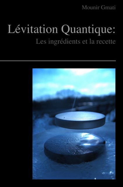
A magnet levitating above a high-temperature 

superconductor, cooled with liquid nitrogen. 

Persistent electric current flows on the surface of 

the superconductor, acting to exclude the 

magnetic field of the magnet (Faraday's law of 

induction). This current effectively forms an 

electromagnet that repels the magnet. 

A high-temperature superconductor levitating 

above a magnet 

held together in pairs by an attraction mediated by lattice phonons. The best available model of high-temperature 

superconductivity is still somewhat crude. There is a hypothesis that electron pairing in high-temperature 

superconductors is mediated by short-range spin waves known as paramagnons. 

Classification 

There is not just one criterion to classify superconductors. The most common are 

• By their physical properties: they can be Type I (if their phase transition is of first order) or Type II (if their 

phase transition is of second order). 

• By the theory to explain them: they can be conventional (if they are explained by the BCS theory or its 

derivatives) or unconventional (if not). 

• By their critical temperature: they can be high temperature (generally considered if they reach the 

superconducting state just cooling them with liquid nitrogen, that is, if T c > 77 K), or low temperature (generally 

if they need other techniques to be cooled under their critical temperature). 

1



• By material: they can be chemical elements (as mercury or lead), alloys (as niobium-titanium or 

germanium-niobium or niobium nitride), ceramics (as YBCO or the magnesium diboride), or organic 

superconductors (as fullerenes or carbon nanotubes, though these examples technically might be included among 

the chemical elements as they are composed entirely of carbon). 

Elementary properties of superconductors 

Most of the physical properties of superconductors vary from material to material, such as the heat capacity and the 

critical temperature, critical field, and critical current density at which superconductivity is destroyed. 

On the other hand, there is a class of properties that are independent of the underlying material. For instance, all 

superconductors have exactly zero resistivity to low applied currents when there is no magnetic field present or if the 

applied field does not exceed a critical value. The existence of these "universal" properties implies that 

superconductivity is a thermodynamic phase, and thus possesses certain distinguishing properties which are largely 

independent of microscopic details. 

Zero electrical DC resistance 

The simplest method to measure the electrical resistance of a sample of 

some material is to place it in an electrical circuit in series with a 

current source I and measure the resulting voltage V across the sample. 

The resistance of the sample is given by Ohm's law as R = V/I. If the 

voltage is zero, this means that the resistance is zero. 

Superconductors are also able to maintain a current with no applied 

voltage whatsoever, a property exploited in superconducting 

electromagnets such as those found in MRI machines. Experiments 

have demonstrated that currents in superconducting coils can persist 

for years without any measurable degradation. Experimental evidence 

points to a current lifetime of at least 100,000 years. Theoretical 

estimates for the lifetime of a persistent current can exceed the 

estimated lifetime of the universe, depending on the wire geometry and the temperature. [1] 

Electric cables for accelerators at CERN: top, 

regular cables for LEP; bottom, superconducting 

cables for the LHC 

In a normal conductor, an electric current may be visualized as a fluid of electrons moving across a heavy ionic 

lattice. The electrons are constantly colliding with the ions in the lattice, and during each collision some of the 

energy carried by the current is absorbed by the lattice and converted into heat, which is essentially the vibrational 

kinetic energy of the lattice ions. As a result, the energy carried by the current is constantly being dissipated. This is 

the phenomenon of electrical resistance. 

The situation is different in a superconductor. In a conventional superconductor, the electronic fluid cannot be 

resolved into individual electrons. Instead, it consists of bound pairs of electrons known as Cooper pairs. This 

pairing is caused by an attractive force between electrons from the exchange of phonons. Due to quantum mechanics, 

the energy spectrum of this Cooper pair fluid possesses an energy gap, meaning there is a minimum amount of 

energy ΔE that must be supplied in order to excite the fluid. Therefore, if ΔE is larger than the thermal energy of the 

lattice, given by kT, where k is Boltzmann's constant and T is the temperature, the fluid will not be scattered by the 

lattice. The Cooper pair fluid is thus a superfluid, meaning it can flow without energy dissipation. 

In a class of superconductors known as type II superconductors, including all known high-temperature 

superconductors, an extremely small amount of resistivity appears at temperatures not too far below the nominal 

superconducting transition when an electric current is applied in conjunction with a strong magnetic field, which 

may be caused by the electric current. This is due to the motion of vortices in the electronic superfluid, which 

dissipates some of the energy carried by the current. If the current is sufficiently small, the vortices are stationary,



and the resistivity vanishes. The resistance due to this effect is tiny compared with that of non-superconducting 

materials, but must be taken into account in sensitive experiments. However, as the temperature decreases far enough 

below the nominal superconducting transition, these vortices can become frozen into a disordered but stationary 

phase known as a "vortex glass". Below this vortex glass transition temperature, the resistance of the material 

becomes truly zero. 

Superconducting phase transition 

In superconducting materials, the 

characteristics of superconductivity 

appear when the temperature T is 

lowered below a critical temperature 

T c . The value of this critical 

temperature varies from material to 

material. Conventional 

superconductors usually have critical 

temperatures ranging from around 

20 K to less than 1 K. Solid mercury, 

for example, has a critical temperature 

of 4.2 K. As of 2009, the highest 

critical temperature found for a 

conventional superconductor is 39 K 

[2] [3] 

for magnesium diboride (MgB ), 

2 

although this material displays enough 

exotic properties that there is some 

Behavior of heat capacity (c v , blue) and resistivity (ρ, green) at the superconducting phase 

transition 

doubt about classifying it as a "conventional" superconductor. [4] Cuprate superconductors can have much higher 

critical temperatures: YBa 2 Cu 3 O 7 , one of the first cuprate superconductors to be discovered, has a critical 

temperature of 92 K, and mercury-based cuprates have been found with critical temperatures in excess of 130 K. The 

explanation for these high critical temperatures remains unknown. Electron pairing due to phonon exchanges 

explains superconductivity in conventional superconductors, but it does not explain superconductivity in the newer 

superconductors that have a very high critical temperature. 

Similarly, at a fixed temperature below the critical temperature, superconducting materials cease to superconduct 

when an external magnetic field is applied which is greater than the critical magnetic field. This is because the Gibbs 

free energy of the superconducting phase increases quadratically with the magnetic field while the free energy of the 

normal phase is roughly independent of the magnetic field. If the material superconducts in the absence of a field, 

then the superconducting phase free energy is lower than that of the normal phase and so for some finite value of the 

magnetic field (proportional to the square root of the difference of the free energies at zero magnetic field) the two 

free energies will be equal and a phase transition to the normal phase will occur. More generally, a higher 

temperature and a stronger magnetic field lead to a smaller fraction of the electrons in the superconducting band and 

consequently a longer London penetration depth of external magnetic fields and currents. The penetration depth 

becomes infinite at the phase transition. 

The onset of superconductivity is accompanied by abrupt changes in various physical properties, which is the 

hallmark of a phase transition. For example, the electronic heat capacity is proportional to the temperature in the 

normal (non-superconducting) regime. At the superconducting transition, it suffers a discontinuous jump and 

thereafter ceases to be linear. At low temperatures, it varies instead as e −α /T for some constant, α. This exponential 

behavior is one of the pieces of evidence for the existence of the energy gap.



The order of the superconducting phase transition was long a matter of debate. Experiments indicate that the 

transition is second-order, meaning there is no latent heat. However in the presence of an external magnetic field 

there is latent heat, as a result of the fact that the superconducting phase has a lower entropy below the critical 

temperature than the normal phase. It has been experimentally demonstrated [5] that, as a consequence, when the 

magnetic field is increased beyond the critical field, the resulting phase transition leads to a decrease in the 

temperature of the superconducting material. 

Calculations in the 1970s suggested that it may actually be weakly first-order due to the effect of long-range 

fluctuations in the electromagnetic field. In the 1980s it was shown theoretically with the help of a disorder field 

theory, in which the vortex lines of the superconductor play a major role, that the transition is of second order within 

the type II regime and of first order (i.e., latent heat) within the type I regime, and that the two regions are separated 

by a tricritical point. [6] The results were confirmed by Monte Carlo computer simulations. [7] 

Meissner effect 

When a superconductor is placed in a weak external magnetic field H, and cooled below its transition temperature, 

the magnetic field is ejected. The Meissner effect does not cause the field to be completely ejected but instead the 

field penetrates the superconductor but only to a very small distance, characterized by a parameter λ, called the 

London penetration depth, decaying exponentially to zero within the bulk of the material. The Meissner effect is a 

defining characteristic of superconductivity. For most superconductors, the London penetration depth is on the order 

of 100 nm. 

The Meissner effect is sometimes confused with the kind of diamagnetism one would expect in a perfect electrical 

conductor: according to Lenz's law, when a changing magnetic field is applied to a conductor, it will induce an 

electric current in the conductor that creates an opposing magnetic field. In a perfect conductor, an arbitrarily large 

current can be induced, and the resulting magnetic field exactly cancels the applied field. 

The Meissner effect is distinct from this—it is the spontaneous expulsion which occurs during transition to 

superconductivity. Suppose we have a material in its normal state, containing a constant internal magnetic field. 

When the material is cooled below the critical temperature, we would observe the abrupt expulsion of the internal 

magnetic field, which we would not expect based on Lenz's law. 

The Meissner effect was given a phenomenological explanation by the brothers Fritz and Heinz London, who 

showed that the electromagnetic free energy in a superconductor is minimized provided 

where H is the magnetic field and λ is the London penetration depth. 

This equation, which is known as the London equation, predicts that the magnetic field in a superconductor decays 

exponentially from whatever value it possesses at the surface. 

A superconductor with little or no magnetic field within it is said to be in the Meissner state. The Meissner state 

breaks down when the applied magnetic field is too large. Superconductors can be divided into two classes according 

to how this breakdown occurs. In Type I superconductors, superconductivity is abruptly destroyed when the strength 

of the applied field rises above a critical value H c . Depending on the geometry of the sample, one may obtain an 

intermediate state [8] consisting of a baroque pattern [9] of regions of normal material carrying a magnetic field mixed 

with regions of superconducting material containing no field. In Type II superconductors, raising the applied field 

past a critical value H c1 leads to a mixed state (also known as the vortex state) in which an increasing amount of 

magnetic flux penetrates the material, but there remains no resistance to the flow of electric current as long as the 

current is not too large. At a second critical field strength H c2 , superconductivity is destroyed. The mixed state is 

actually caused by vortices in the electronic superfluid, sometimes called fluxons because the flux carried by these 

vortices is quantized. Most pure elemental superconductors, except niobium, technetium, vanadium and carbon 

nanotubes, are Type I, while almost all impure and compound superconductors are Type II.



London moment 

Conversely, a spinning superconductor generates a magnetic field, precisely aligned with the spin axis. The effect, 

the London moment, was put to good use in Gravity Probe B. This experiment measured the magnetic fields of four 

superconducting gyroscopes to determine their spin axes. This was critical to the experiment since it is one of the 

few ways to accurately determine the spin axis of an otherwise featureless sphere. 

Theories of superconductivity 

Since the discovery of superconductivity, great efforts have been devoted to finding out how and why it works. 

During the 1950s, theoretical condensed matter physicists arrived at a solid understanding of "conventional" 

superconductivity, through a pair of remarkable and important theories: the phenomenological Ginzburg-Landau 

theory (1950) and the microscopic BCS theory (1957). [10] [11] Generalizations of these theories form the basis for 

understanding the closely related phenomenon of superfluidity, because they fall into the Lambda transition 

universality class, but the extent to which similar generalizations can be applied to unconventional superconductors 

as well is still controversial. The four-dimensional extension of the Ginzburg-Landau theory, the Coleman-Weinberg 

model, is important in quantum field theory and cosmology. 

London theory 

The first phenomenological theory of superconductivity was London theory. It was put forward by the brothers Fritz 

and Heinz London in 1935, shortly after the discovery that magnetic fields are expelled from superconductors. A 

major triumph of the equations of this theory is their ability to explain the Meissner effect [12] , wherein a material 

exponentially expels all internal magnetic fields as it crosses the superconducting threshold. By using the London 

equation, one can obtain the dependence of the magnetic field inside the superconductor on the distance to the 

surface [13] . 

There are two London equations: 

The first equation follows from the Newton's second law for superconducting electrons. 

History of superconductivity 

Superconductivity was discovered on April 8, 1911 by Heike Kamerlingh Onnes, who was studying the resistance of 

solid mercury at cryogenic temperatures using the recently-produced liquid helium as a refrigerant. At the 

temperature of 4.2 K, he observed that the resistance abruptly disappeared. [14] In the same experiment, he also 

observed the superfluid transition of helium at 2.2 K, without recognizing its significance. (The precise date and 

circumstances of the discovery were only reconstructed a century later, when Onnes's notebook was found.) [15] In 

subsequent decades, superconductivity was observed in several other materials. In 1913, lead was found to 

superconduct at 7 K, and in 1941 niobium nitride was found to superconduct at 16 K. 

The next important step in understanding superconductivity occurred in 1933, when Meissner and Ochsenfeld 

discovered that superconductors expelled applied magnetic fields, a phenomenon which has come to be known as the 

Meissner effect. [16] In 1935, F. and H. London showed that the Meissner effect was a consequence of the 

minimization of the electromagnetic free energy carried by superconducting current. [17] 

In 1950, the phenomenological Ginzburg-Landau theory of superconductivity was devised by Landau and 

Ginzburg. [18] This theory, which combined Landau's theory of second-order phase transitions with a 

Schrödinger-like wave equation, had great success in explaining the macroscopic properties of superconductors. In 

particular, Abrikosov showed that Ginzburg-Landau theory predicts the division of superconductors into the two 

categories now referred to as Type I and Type II. Abrikosov and Ginzburg were awarded the 2003 Nobel Prize for



their work (Landau had received the 1962 Nobel Prize for other work, and died in 1968). 

Also in 1950, Maxwell and Reynolds et al. found that the critical temperature of a superconductor depends on the 

isotopic mass of the constituent element. [19] [20] This important discovery pointed to the electron-phonon interaction 

as the microscopic mechanism responsible for superconductivity. 

The complete microscopic theory of superconductivity was finally proposed in 1957 by Bardeen, Cooper and 

Schrieffer. [11] Independently, the superconductivity phenomenon was explained by Nikolay Bogolyubov. This BCS 

theory explained the superconducting current as a superfluid of Cooper pairs, pairs of electrons interacting through 

the exchange of phonons. For this work, the authors were awarded the Nobel Prize in 1972. 

The BCS theory was set on a firmer footing in 1958, when Bogolyubov showed that the BCS wavefunction, which 

had originally been derived from a variational argument, could be obtained using a canonical transformation of the 

electronic Hamiltonian. [21] In 1959, Lev Gor'kov showed that the BCS theory reduced to the Ginzburg-Landau 

theory close to the critical temperature. [22] 

In 1962, the first commercial superconducting wire, a niobium-titanium alloy, was developed by researchers at 

Westinghouse, allowing the construction of the first practical superconducting magnets. In the same year, Josephson 

made the important theoretical prediction that a supercurrent can flow between two pieces of superconductor 

separated by a thin layer of insulator. [23] This phenomenon, now called the Josephson effect, is exploited by 

superconducting devices such as SQUIDs. It is used in the most accurate available measurements of the magnetic 

flux quantum , and thus (coupled with the quantum Hall resistivity) for Planck's constant h. Josephson 

was awarded the Nobel Prize for this work in 1973. 

In 2008, it was discovered that the same mechanism that produces superconductivity could produce a superinsulator 

state in some materials, with almost infinite electrical resistance. [24] 

High-temperature superconductivity 

Until 1986, physicists had believed that BCS theory forbade superconductivity at temperatures above about 30 K. In 

that year, Bednorz and Müller discovered superconductivity in a lanthanum-based cuprate perovskite material, which 

had a transition temperature of 35 K (Nobel Prize in Physics, 1987). [25] It was soon found that replacing the 

lanthanum with yttrium (i.e., making YBCO) raised the critical temperature to 92 K, which was important because 

liquid nitrogen could then be used as a refrigerant (the boiling point of nitrogen is 77 K at atmospheric pressure). [26] 

This is important commercially because liquid nitrogen can be produced cheaply on-site from air, and is not prone to 

some of the problems (for instance solid air plugs) of helium in piping. Many other cuprate superconductors have 

since been discovered, and the theory of superconductivity in these materials is one of the major outstanding 

challenges of theoretical condensed matter physics. [27] 

From about 1993, the highest temperature superconductor was a ceramic material consisting of thallium, mercury, 

copper, barium, calcium and oxygen (HgBa 2 Ca 2 Cu 3 O 8+δ ) with T c = 138 K. [28] 

In February 2008, an iron-based family of high-temperature superconductors was discovered. [29] [30] Hideo Hosono, 

of the Tokyo Institute of Technology, and colleagues found lanthanum oxygen fluorine iron arsenide 

(LaO 1-x F x FeAs), an oxypnictide that superconducts below 26 K. Replacing the lanthanum in LaO 1−x F x FeAs with 

samarium leads to superconductors that work at 55 K. [31]



Crystal structure of high-temperature ceramic superconductors 

The structure of a high-T c superconductor is closely related to perovskite structure, and the structure of these 

compounds has been described as a distorted, oxygen deficient multi-layered perovskite structure. One of the 

properties of the crystal structure of oxide superconductors is an alternating multi-layer of CuO 2 planes with 

superconductivity taking place between these layers. The more layers of CuO 2 the higher T c . This structure causes a 

large anisotropy in normal conducting and superconducting properties, since electrical currents are carried by holes 

induced in the oxygen sites of the CuO 2 sheets. The electrical conduction is highly anisotropic, with a much higher 

conductivity parallel to the CuO 2 plane than in the perpendicular direction. Generally, Critical temperatures depend 

on the chemical compositions, cations substitutions and oxygen content. They can be classified as superstripes; i.e., 

particular realizations of superlattices at atomic limit made of superconducting atomic layers, wires, dots separated 

by spacer layers, that gives multiband and multigap superconductivity. 

YBaCuO superconductors 

The first superconductor found with T c > 77 K (liquid nitrogen boiling 

point) is yttrium barium copper oxide (YBa 2 Cu 3 O 7-x ), the proportions 

of the 3 different metals in the YBa 2 Cu 3 O 7 superconductor are in the 

mole ratio of 1 to 2 to 3 for yttrium to barium to copper respectively. 

Thus, this particular superconductor is often referred to as the 123 

superconductor. 

The unit cell of YBa 2 Cu 3 O 7 consists of three pseudocubic elementary 

perovskite unit cells. Each perovskite unit cell contains a Y or Ba atom 

at the center: Ba in the bottom unit cell, Y in the middle one, and Ba in 

the top unit cell. Thus, Y and Ba are stacked in the sequence 

[Ba–Y–Ba] along the c-axis. All corner sites of the unit cell are 

occupied by Cu, which has two different coordinations, Cu(1) and 

Cu(2), with respect to oxygen. There are four possible crystallographic 

sites for oxygen: O(1), O(2), O(3) and O(4). [32] The coordination 

polyhedra of Y and Ba with respect to oxygen are different. The 

tripling of the perovskite unit cell leads to nine oxygen atoms, whereas 

YBa 2 Cu 3 O 7 has seven oxygen atoms and, therefore, is referred to as an 

oxygen-deficient perovskite structure. The structure has a stacking of 

YBCO unit cell 

different layers: (CuO)(BaO)(CuO 2 )(Y)(CuO 2 )(BaO)(CuO). One of the key feature of the unit cell of YBa 2 Cu 3 O 7-x 

(YBCO) is the presence of two layers of CuO 2 . The role of the Y plane is to serve as a spacer between two CuO 2 

planes. In YBCO, the Cu–O chains are known to play an important role for superconductivity. T c is maximal near 92 

K when x ≈ 0.15 and the structure is orthorhombic. Superconductivity disappears at x ≈ 0.6, where the structural 

transformation of YBCO occurs from orthorhombic to tetragonal. [33]



Bi-, Tl- and Hg-based high-T c superconductors 

The crystal structure of Bi-, Tl- and Hg-based high-T c superconductors are very similar. Like YBCO, the 

perovskite-type feature and the presence of CuO 2 layers also exist in these superconductors. However, unlike YBCO, 

Cu–O chains are not present in these superconductors. The YBCO superconductor has an orthorhombic structure, 

whereas the other high-T c superconductors have a tetragonal structure. 

The Bi–Sr–Ca–Cu–O system has three superconducting phases forming a homologous series as 

Bi 2 Sr 2 Ca n−1 Cu n O 4+2n+x (n = 1, 2 and 3). These three phases are Bi-2201, Bi-2212 and Bi-2223, having transition 

temperatures of 20, 85 and 110 K, respectively, where the numbering system represent number of atoms for Bi, Sr, 

Ca and Cu respectively. [34] The two phases have a tetragonal structure which consists of two sheared 

crystallographic unit cells. The unit cell of these phases has double Bi–O planes which are stacked in a way that the 

Bi atom of one plane sits below the oxygen atom of the next consecutive plane. The Ca atom forms a layer within the 

interior of the CuO 2 layers in both Bi-2212 and Bi-2223; there is no Ca layer in the Bi-2201 phase. The three phases 

differ with each other in the number of CuO 2 planes; Bi-2201, Bi-2212 and Bi-2223 phases have one, two and three 

CuO 2 planes, respectively. The c axis of these phases increases with the number of CuO 2 planes (see table below). 

The coordination of the Cu atom is different in the three phases. The Cu atom forms an octahedral coordination with 

respect to oxygen atoms in the 2201 phase, whereas in 2212, the Cu atom is surrounded by five oxygen atoms in a 

pyramidal arrangement. In the 2223 structure, Cu has two coordinations with respect to oxygen: one Cu atom is 

bonded with four oxygen atoms in square planar configuration and another Cu atom is coordinated with five oxygen 

atoms in a pyramidal arrangement. [35] 

Tl–Ba–Ca–Cu–O superconductor: The first series of the Tl-based superconductor containing one Tl–O layer has 

the general formula TlBa 2 Ca n-1 Cu n O 2n+3 , [36] whereas the second series containing two Tl–O layers has a formula of 

Tl 2 Ba 2 Ca n-1 Cu n O 2n+4 with n = 1, 2 and 3. In the structure of Tl 2 Ba 2 CuO 6 (Tl-2201), there is one CuO 2 layer with 

the stacking sequence (Tl–O) (Tl–O) (Ba–O) (Cu–O) (Ba–O) (Tl–O) (Tl–O). In Tl 2 Ba 2 CaCu 2 O 8 (Tl-2212), there 

are two Cu–O layers with a Ca layer in between. Similar to the Tl 2 Ba 2 CuO 6 structure, Tl–O layers are present 

outside the Ba–O layers. In Tl 2 Ba 2 Ca 2 Cu 3 O 10 (Tl-2223), there are three CuO2 layers enclosing Ca layers between 

each of these. In Tl-based superconductors, T c is found to increase with the increase in CuO 2 layers. However, the 

value of T c decreases after four CuO 2 layers in TlBa 2 Ca n-1 Cu n O 2n+3 , and in the Tl 2 Ba 2 Ca n-1 Cu n O 2n+4 compound, it 

decreases after three CuO 2 layers. [37] 

Hg–Ba–Ca–Cu–O superconductor: The crystal structure of HgBa 2 CuO 4 (Hg-1201), [38] HgBa 2 CaCu 2 O 6 

(Hg-1212) and HgBa 2 Ca 2 Cu 3 O 8 (Hg-1223) is similar to that of Tl-1201, Tl-1212 and Tl-1223, with Hg in place 

of Tl. It is noteworthy that the T c of the Hg compound (Hg-1201) containing one CuO 2 layer is much larger as 

compared to the one-CuO 2 -layer compound of thallium (Tl-1201). In the Hg-based superconductor, T c is also found 

to increase as the CuO 2 layer increases. For Hg-1201, Hg-1212 and Hg-1223, the values of T c are 94, 128 and 134 K 

respectively, as shown in table below. The observation that the T c of Hg-1223 increases to 153 K under high pressure 

indicates that the T c of this compound is very sensitive to the structure of the compound. [39]



Critical temperature (T c ), crystal structure and lattice constants of some high-T c 

superconductors 

Formula Notation T c (K) No. of Cu-O 

YBa 2 Cu 3 O 7 

Bi 2 Sr 2 CuO 6 

Bi 2 Sr 2 CaCu 2 O 8 

Bi 2 Sr 2 Ca 2 Cu 3 O 6 

Tl 2 Ba 2 CuO 6 

Tl 2 Ba 2 CaCu 2 O 8 

Tl 2 Ba 2 Ca 2 Cu 3 O 10 

TlBa 2 Ca 3 Cu 4 O 11 

HgBa 2 CuO 4 

HgBa 2 CaCu 2 O 6 

Preparation of high-T c superconductors 

planes 

in unit cell 

Crystal structure 

123 92 2 Orthorhombic 

Bi-2201 20 1 Tetragonal 



Tl-2201 80 1 Tetragonal 




Hg-1201 94 1 Tetragonal 

Hg-1212 128 2 Tetragonal 

HgBa 2 Ca 2 Cu 3 O 8 Hg-1223 134 3 Tetragonal 

The simplest method for preparing high-T c superconductors is a 

solid-state thermochemical reaction involving mixing, calcination and 

sintering. The appropriate amounts of precursor powders, usually 

oxides and carbonates, are mixed thoroughly using a ball mill. Solution 

chemistry processes such as coprecipitation, freeze-drying and sol-gel 

methods are alternative ways for preparing a homogenous mixture. 

These powders are calcined in the temperature range from 800 °C to 

950 °C for several hours. The powders are cooled, reground and 

calcined again. This process is repeated several times to get 

homogenous material. The powders are subsequently compacted to 

Superconductor timeline 

pellets and sintered. The sintering environment such as temperature, annealing time, atmosphere and cooling rate 

play a very important role in getting good high-T c superconducting materials. The YBa 2 Cu 3 O 7-x compound is 

prepared by calcination and sintering of a homogenous mixture of Y 2 O 3 , BaCO 3 and CuO in the appropriate atomic 

ratio. Calcination is done at 900–950 °C, whereas sintering is done at 950 °C in an oxygen atmosphere. The oxygen 

stoichiometry in this material is very crucial for obtaining a superconducting YBa 2 Cu 3 O 7−x compound. At the time 

of sintering, the semiconducting tetragonal YBa 2 Cu 3 O 6 compound is formed, which, on slow cooling in oxygen 

atmosphere, turns into superconducting YBa 2 Cu 3 O 7−x . The uptake and loss of oxygen are reversible in 

YBa 2 Cu 3 O 7−x . A fully oxidized orthorhombic YBa 2 Cu 3 O 7−x sample can be transformed into tetragonal YBa 2 Cu 3 O 6 

by heating in a vacuum at temperature above 700 °C. [33] 

The preparation of Bi-, Tl- and Hg-based high-T c superconductors is difficult compared to YBCO. Problems in these 

superconductors arise because of the existence of three or more phases having a similar layered structure. Thus, 

syntactic intergrowth and defects such as stacking faults occur during synthesis and it becomes difficult to isolate a 

single superconducting phase. For Bi–Sr–Ca–Cu–O, it is relatively simple to prepare the Bi-2212 (T c ≈ 85 K) phase, 

whereas it is very difficult to prepare a single phase of Bi-2223 (T c ≈ 110 K). The Bi-2212 phase appears only after 

few hours of sintering at 860–870 °C, but the larger fraction of the Bi-2223 phase is formed after a long reaction



time of more than a week at 870 °C. [35] Although the substitution of Pb in the Bi–Sr–Ca–Cu–O compound has been 

found to promote the growth of the high-T c phase, [40] a long sintering time is still required. 

Possible superconductivity of the vacuum 

Maxim Chernodub of the French National Centre for Scientific Research has postulated that the vacuum can become 

a superconductor in magnetic fields of 10 16 Tesla or more, [41] at temperatures of at least a billion, [42] perhaps billions 

of degrees. [43] 

Applications 

Superconducting magnets are some of the most powerful electromagnets known. They are used in MRI/NMR 

machines, mass spectrometers, and the beam-steering magnets used in particle accelerators. They can also be used 

for magnetic separation, where weakly magnetic particles are extracted from a background of less or non-magnetic 

particles, as in the pigment industries. 

In the 1950s and 1960s, superconductors were used to build experimental digital computers using cryotron switches. 

More recently, superconductors have been used to make digital circuits based on rapid single flux quantum 

technology and RF and microwave filters for mobile phone base stations. 

Superconductors are used to build Josephson junctions which are the building blocks of SQUIDs (superconducting 

quantum interference devices), the most sensitive magnetometers known. SQUIDs are used in scanning SQUID 

microscopes and magnetoencephalography. Series of Josephson devices are used to realize the SI volt. Depending on 

the particular mode of operation, a superconductor-insulator-superconductor Josephson junction can be used as a 

photon detector or as a mixer. The large resistance change at the transition from the normal- to the superconducting 

state is used to build thermometers in cryogenic micro-calorimeter photon detectors. The same effect is used in 

ultrasensitive bolometers made from superconducting materials. 

Other early markets are arising where the relative efficiency, size and weight advantages of devices based on 

high-temperature superconductivity outweigh the additional costs involved. 

Promising future applications include high-performance smart grid, electric power transmission, transformers, power 

storage devices, electric motors (e.g. for vehicle propulsion, as in vactrains or maglev trains), magnetic levitation 

devices, fault current limiters, nanoscopic materials such as buckyballs, nanotubes, composite materials and 

superconducting magnetic refrigeration. However, superconductivity is sensitive to moving magnetic fields so 

applications that use alternating current (e.g. transformers) will be more difficult to develop than those that rely upon 

direct current. 

Nobel Prize for Superconductivity 

1913 Heike Kamerlingh Onnes on Matter at low temperature 

1972 John Bardeen, Leon N. Cooper, J. Robert Schrieffer on Theory of superconductivity 

1973 Leo Esaki, Ivar Giaever, Brian D. Josephson on Tunneling in superconductors 

1987 Georg Bednorz, Alex K. Müller on High-temperature superconductivity 

2003 Alexei A. Abrikosov, Vitaly L. Ginzburg, Anthony J. Leggett on Pioneering contributions to the theory of 

superconductors and superfluids. [44]



References 

[1] John C. Gallop (1990). SQUIDS, the Josephson Effects and Superconducting Electronics (http:/ / books. google. com/ ?id=ad8_JsfCdKQC& 

printsec=frontcover). CRC Press. pp. 3, 20. ISBN 0750300515. . 

[2] Jun Nagamatsu, Norimasa Nakagawa, Takahiro Muranaka, Yuji Zenitani and Jun Akimitsu (2001). "Superconductivity at 39 K in magnesium 

diboride". Nature 410 (6824): 63. Bibcode 2001Natur.410...63N. doi:10.1038/35065039. PMID 11242039. 

[3] Paul Preuss (14 August 2002). "A most unusual superconductor and how it works: first-principles calculation explains the strange behavior of 

magnesium diboride" (http:/ / www. lbl. gov/ Science-Articles/ Archive/ MSD-superconductor-Cohen-Louie. html). Research News 

(Lawrence Berkeley National Laboratory). . Retrieved 2009-10-28. 

[4] Hamish Johnston (17 February 2009). "Type-1.5 superconductor shows its stripes" (http:/ / physicsworld. com/ cws/ article/ news/ 37806). 

Physics World (Institute of Physics). . Retrieved 2009-10-28. 

[5] R. L. Dolecek (1954). "Adiabatic Magnetization of a Superconducting Sphere". Physical Review 96 (1): 25–28. 

Bibcode 1954PhRv...96...25D. doi:10.1103/PhysRev.96.25. 

[6] H. Kleinert (1982). "Disorder Version of the Abelian Higgs Model and the Order of the Superconductive Phase Transition" (http:/ / www. 

physik. fu-berlin. de/ ~kleinert/ 97/ 97. pdf). Lettere al Nuovo Cimento 35 (13): 405–412. doi:10.1007/BF02754760. . 

[7] J. Hove, S. Mo, A. Sudbo (2002). "Vortex interactions and thermally induced crossover from type-I to type-II superconductivity" (http:/ / 

www. physik. fu-berlin. de/ ~kleinert/ papers/ sudbotre064524. pdf). Physical Review B 66 (6): 064524. arXiv:cond-mat/0202215. 

Bibcode 2002PhRvB..66f4524H. doi:10.1103/PhysRevB.66.064524. . 

[8] Lev D. Landau, Evgeny M. Lifschitz (1984). Electrodynamics of Continuous Media. Course of Theoretical Physics. 8. Oxford: 

Butterworth-Heinemann. ISBN 0-7506-2634-8. 

[9] David J. E. Callaway (1990). "On the remarkable structure of the superconducting intermediate state". Nuclear Physics B 344 (3): 627–645. 

Bibcode 1990NuPhB.344..627C. doi:10.1016/0550-3213(90)90672-Z. 

[10] J. Bardeen, L. N. Cooper and J. R. Schrieffer (1957). "Microscopic Theory of Superconductivity". Physical Review 106 (1): 162–164. 

Bibcode 1957PhRv..106..162B. doi:10.1103/PhysRev.106.162. 

[11] J. Bardeen, L. N. Cooper and J. R. Schrieffer (1957). "Theory of Superconductivity". Physical Review 108 (5): 1175–1205. 

Bibcode 1957PhRv..108.1175B. doi:10.1103/PhysRev.108.1175. 

[12] Meissner, W.; R. Ochsenfeld (1933). "Ein neuer Effekt bei Eintritt der Supraleitfähigkeit". Naturwissenschaften 21 (44): 787. 

Bibcode 1933NW.....21..787M. doi:10.1007/BF01504252. 

[13] "The London equations" (http:/ / openlearn. open. ac. uk/ mod/ oucontent/ view. php?id=398540& section=3. 3). The Open University. . 

Retrieved 2011-10-16. 

[14] H. K. Onnes (1911). "The resistance of pure mercury at helium temperatures". Commun. Phys. Lab. Univ. Leiden 12: 120. 

[15] The Discovery of Superconductivity (http:/ / ilorentz. org/ history/ cold/ DelftKes_HKO_PT. pdf) 

[16] W. Meissner and R. Ochsenfeld (1933). "Ein neuer Effekt bei Eintritt der Supraleitfähigkeit". Naturwissenschaften 21 (44): 787–788. 

Bibcode 1933NW.....21..787M. doi:10.1007/BF01504252. 

[17] F. London and H. London (1935). "The Electromagnetic Equations of the Supraconductor". Proceedings of the Royal Society of London A 

149 (866): 71–88. Bibcode 1935RSPSA.149...71L. doi:10.1098/rspa.1935.0048. JSTOR 96265. 

[18] V. L. Ginzburg and L.D. Landau (1950). "On the theory of superconductivity". Zhurnal Eksperimental'noi i Teoreticheskoi Fiziki 20: 1064. 

[19] E. Maxwell (1950). "Isotope Effect in the Superconductivity of Mercury". Physical Review 78 (4): 477. Bibcode 1950PhRv...78..477M. 

doi:10.1103/PhysRev.78.477. 

[20] C. A. Reynolds, B. Serin, W. H. Wright and L. B. Nesbitt (1950). "Superconductivity of Isotopes of Mercury". Physical Review 78 (4): 487. 

Bibcode 1950PhRv...78..487R. doi:10.1103/PhysRev.78.487. 

[21] N. N. Bogoliubov (1958). "A new method in the theory of superconductivity". Zhurnal Eksperimental'noi i Teoreticheskoi Fiziki 34: 58. 

[22] L. P. Gor'kov (1959). "Microscopic derivation of the Ginzburg--Landau equations in the theory of superconductivity". Zhurnal 

Eksperimental'noi i Teoreticheskoi Fiziki 36: 1364. 

[23] B. D. Josephson (1962). "Possible new effects in superconductive tunnelling". Physics Letters 1 (7): 251–253. Bibcode 1962PhL.....1..251J. 

doi:10.1016/0031-9163(62)91369-0. 

[24] "Newly discovered fundamental state of matter, a superinsulator, has been created." (http:/ / www. sciencedaily. com/ releases/ 2008/ 04/ 

080408160614. htm). Science Daily. April 9, 2008. . Retrieved 2008-10-23. 

[25] J. G. Bednorz and K. A. Mueller (1986). "Possible high T C superconductivity in the Ba-La-Cu-O system". Zeitschrift für Physik B 64 (2): 

189–193. Bibcode 1986ZPhyB..64..189B. doi:10.1007/BF01303701. 

[26] M. K. Wu et al. (1987). "Superconductivity at 93 K in a New Mixed-Phase Y-Ba-Cu-O Compound System at Ambient Pressure". Physical 

Review Letters 58 (9): 908–910. Bibcode 1987PhRvL..58..908W. doi:10.1103/PhysRevLett.58.908. PMID 10035069. 

[27] Alexei A. Abrikosov (8 December 2003). "type II Superconductors and the Vortex Lattice" (http:/ / nobelprize. org/ nobel_prizes/ physics/ 

laureates/ 2003/ abrikosov-lecture. html). Nobel Lecture. . 

[28] P. Dai, B. C. Chakoumakos, G. F. Sun, K. W. Wong, Y. Xin and D. F. Lu (1995). "Synthesis and neutron powder diffraction study of the 

superconductor HgBa 2 Ca 2 Cu 3 O 8+δ by Tl substitution". Physica C 243 (3–4): 201–206. Bibcode 1995PhyC..243..201D. 

doi:10.1016/0921-4534(94)02461-8. 

[29] Hiroki Takahashi, Kazumi Igawa, Kazunobu Arii, Yoichi Kamihara, Masahiro Hirano, Hideo Hosono (2008). "Superconductivity at 43 K in 

an iron-based layered compound LaO 1−x F x FeAs". Nature 453 (7193): 376–378. Bibcode 2008Natur.453..376T. doi:10.1038/nature06972.



PMID 18432191. 

[30] Adrian Cho. "Second Family of High-Temperature Superconductors Discovered" (http:/ / sciencenow. sciencemag. org/ cgi/ content/ full/ 

2008/ 417/ 1). ScienceNOW Daily News. . 

[31] Zhi-An Ren et al. (2008). "Superconductivity and phase diagram in iron-based arsenic-oxides ReFeAsO1-d (Re = rare-earth metal) without 

fluorine doping". EPL 83: 17002. Bibcode 2008EL.....8317002R. doi:10.1209/0295-5075/83/17002. 

[32] R. Hazen et al. (1987). "Crystallographic description of phases in the Y-Ba-Cu-O superconductor". Physical Review B 35 (13): 7238. 

Bibcode 1987PhRvB..35.7238H. doi:10.1103/PhysRevB.35.7238. 

[33] Neeraj Khare (2003-05-01). Handbook of High-Temperature Superconductor Electronics (http:/ / books. google. com/ 

books?id=is-L_R2H3IAC). ISBN 0-8247-0823-7. . 

[34] R. Hazen et al. (1988). "Superconductivity in the high-T c Bi-Ca-Sr-Cu-O system: Phase identification". Physical Review Letters 60 (12): 

1174. Bibcode 1988PhRvL..60.1174H. doi:10.1103/PhysRevLett.60.1174. 

[35] J. Tarascon et al. (1988). "Preparation, structure, and properties of the superconducting compound series Bi 2 Sr 2 Ca n−1 Cu n O y with n = 1, 2, 

and 3". Physical Review B 38 (13): 8885. Bibcode 1988PhRvB..38.8885T. doi:10.1103/PhysRevB.38.8885. 

[36] Z. Sheng et al. (1988). "Superconductivity at 90 K in the Tl-Ba-Cu-O system". Physical Review Letters 60 (10): 937–940. 

Bibcode 1988PhRvL..60..937S. doi:10.1103/PhysRevLett.60.937. PMID 10037895. 

[37] Z.Z. Sheng, A. M. Hermann, Z. Z.; Hermann, A. M. (1988). "Superconductivity in the rare-earth-free Tl-Ba-Cu-O system above 

liquid-nitrogen temperature". Nature 332 (6159): 55. Bibcode 1988Natur.332...55S. doi:10.1038/332055a0. 

[38] S. N. Putilin et al. (1993). "Superconductivity at 94 K in HgBa2Cu04+δ". Nature 362 (6417): 226. Bibcode 1993Natur.362..226P. 

doi:10.1038/362226a0. 

[39] C. W. Chu et al. (1993). "Superconductivity above 150 K in HgBa2Ca2Cu3O8+δ at high pressures". Nature 365 (6444): 323. 

Bibcode 1993Natur.365..323C. doi:10.1038/365323a0. 

[40] D. Shi et al. (1989). "Origin of enhanced growth of the 110 K superconducting phase by Pb doping in the Bi-Sr-Ca-Cu-O system". Applied 

Physics Letters 55 (7): 699. Bibcode 1989ApPhL..55..699S. doi:10.1063/1.101573. 

[41] Maggie McKee: How to turn the vacuum into a superconductor (http:/ / webcache. googleusercontent. com/ 

search?q=cache:yuuQSPuvjdAJ:www. newscientist. com/ article/ mg21028073. 800-how-to-turn-the-vacuum-into-a-superconductor. html+ 

"maxim+ chernodub"+ "new+ scientist"& cd=4& hl=en& ct=clnk& gl=uk& source=www. google. co. uk). New Scientist, April 8, 2011, 

retrieved May 13, 2011 

[42] Alasdair Wilkins: Ultra-hot superconductors could spontaneously form in the vacuum of space (http:/ / io9. com/ 5787141/ ultra+ 

hot-superconductors-could-spontaneously-form-in-the-vacuum-of-space). io9, March 30, 2011, retrieved May 13, 2011 

[43] Jon Cartwright: Superconductivity from nowhere (http:/ / physicsworld. com/ cws/ article/ news/ 45558). Physicworld.com, March 29, 2011, 

retrieved May 13, 2011 

[44] The Nobel Prize for Physics, 1901–2008 [=http:/ / math. ucr. edu/ home/ baez/ physics/ Administrivia/ nobel. html "The Nobel Prize for 

Physics,1901-2008"]. =. 

Further reading 

• Hagen Kleinert (1989). "Superflow and Vortex Lines" (http:/ / www. physik. fu-berlin. de/ ~kleinert/ 

kleiner_reb1/ contents1. html). Gauge Fields in Condensed Matter. 1. World Scientific. ISBN 9971-5-0210-0. 

• Anatoly Larkin; Andrei Varlamov (2005). Theory of Fluctuations in Superconductors. Oxford University Press. 

ISBN 0198528159. 

• A. G. Lebed (2008). The Physics of Organic Superconductors and Conductors. 110 (1rst ed.). Springer. 

ISBN 978-3-540-76667-4. 

• Jean Matricon, Georges Waysand, Charles Glashausser (2003). The Cold Wars: A History of Superconductivity. 

Rutgers University Press. ISBN 0813532957. 

• "Physicist Discovers Exotic Superconductivity" (http:/ / www. sciencedaily. com/ releases/ 2006/ 08/ 

060817101658. htm). ScienceDaily. 17 August 2006. 

• Michael Tinkham (2004). Introduction to Superconductivity (2nd ed.). Dover Books. ISBN 0-486-43503-2. 

• Terry Orlando, Kevin Delin (1991). Foundations of Applied Superconductivity. Prentice Hall. 

ISBN 978-0-2011-8323-8. 

• Paul Tipler, Ralph Llewellyn (2002). Modern Physics (4th ed.). W. H. Freeman. ISBN 0-7167-4345-0.



External links 

• Everything about superconductivity: properties, research, applications with videos, animations, games (http:/ / 

www. superconductivity. eu) 

• Video about Type I Superconductors: R=0/transition temperatures/ B is a state variable/ Meissner effect/ Energy 

gap(Giaever)/ BCS model (http:/ / alfredleitner. com) 

• Superconductivity: Current in a Cape and Thermal Tights. An introduction to the topic for non-scientists (http:/ / 

www. magnet. fsu. edu/ education/ tutorials/ magnetacademy/ superconductivity101/ ) National High Magnetic 

Field Laboratory 

• Introduction to superconductivity (http:/ / www. ornl. gov/ reports/ m/ ornlm3063r1/ pt1. html) 

• Lectures on Superconductivity (series of videos, including interviews with leading experts) (http:/ / www. msm. 

cam. ac. uk/ ascg/ lectures/ ) 

• Superconducting Niobium Cavities (http:/ / www. sns. gov/ partnerlabs/ jlab. shtml) 

• Superconductivity in everyday life : Interactive exhibition (http:/ / www. superlife. info) 

• Videos for various types of superconducting levitations including trains and hoolahoops – also videos of Ohm's 

law in a superconductor (http:/ / h0. web. u-psud. fr/ supraconductivite/ vulgaFilms. html) 

• Video of the Meissner effect from the NJIT Mathclub (http:/ / web. njit. edu/ ~mathclub/ superconductor/ index. 

html) 

• Superconductivity News Update (http:/ / www. superconductivitynewsupdate. com) 

• Superconductor Week Newsletter – industry news, links, et cetera (http:/ / www. superconductorweek. com) 

• Superconducting Magnetic Levitation (http:/ / www. maniacworld. com/ Superconducting-Magnetic-Levitation. 

html) 

• National Superconducting Cyclotron Laboratory at Michigan State University (http:/ / www. nscl. msu. edu) 

• High Temperature Superconducting and Cryogenics in RF applications (http:/ / www. suptech. com/ 

hts_crfe_tech. htm) 

• CERN Superconductors Database (http:/ / sdb-server. cern. ch/ mediawiki/ index. php/ Main_Page) 

• Magnetisation of High Temperature superconductors by the flux pumping method (http:/ / www. fluxpump. co. 

uk/ default. aspx) 

• YouTube Video Levitating magnet (http:/ / youtube. com/ watch?v=indyz6O-Xyw& feature=user) 

• Isotope effect in superconductivity (http:/ / www. physics. csulb. edu/ ~abill/ isotope. html) 

• International Workshop on superconductivity in Diamond and Related Materials (free download papers) (http:/ / 

www. iop. org/ EJ/ toc/ 1468-6996/ 9/ 4) 

• New Diamond and Frontier Carbon Technology Volume 17, No.1 Special Issue on Superconductivity in CVD 

Diamond (http:/ / www. nims. go. jp/ NFM/ NDFCT17/ NDFCT17. html) 

• DoITPoMS Teaching and Learning Package – "Superconductivity" (http:/ / www. doitpoms. ac. uk/ tlplib/ 

superconductivity/ index. php) 

• The Nobel Prize for Physics, 1901–2008 (http:/ / math. ucr. edu/ home/ baez/ physics/ Administrivia/ nobel. html)


Type-I superconductor 14 

Type-I superconductor 

Superconductors cannot be penetrated by magnetic flux lines (Meissner–Ochsenfeld effect). This Meissner state 

breaks down when the applied magnetic field is too large. Superconductors can be divided into two classes according 

to how this breakdown occurs. In Type-I superconductors, superconductivity is abruptly destroyed via a first order 

phase transition when the strength of the applied field rises above a critical value H c . As such, they have only a 

single critical magnetic field at which the material ceases to superconduct, becoming resistive. Depending on the 

geometry of the sample, one may obtain an intermediate state described first by Lev Landau [1] consisting of a 

baroque pattern [2] of macroscopically large regions of normal material carrying a magnetic field mixed with regions 

of superconducting material containing no field. Elementary superconductors, such as aluminium and lead are 

typical Type-I superconductors. The origin of their superconductivity is explained by BCS theory. This type of 

superconductivity is normally exhibited by pure metals, e.g. aluminium, lead or mercury. 

References 

[1] L.D. Landau (1984). Electrodynamics of Continuous Media. Course of Theoretical Physics. Vol. 8. Butterworth-Heinemann. 

ISBN 0-7506-2634-8. 

[2] D.J.E. Callaway (1990). "On the remarkable structure of the superconducting intermediate state". Nuclear Physics B 344: 627–645. 

Bibcode 1990NuPhB.344..627C. doi:10.1016/0550-3213(90)90672-Z.



Yttrium barium copper oxide 

CAS number 

Yttrium barium copper oxide 

Identifiers 

Properties 

107539-20-8 [1] 

Molecular formula YBa 2 Cu 3 O 7 

Molar mass 666.19 

Appearance Black solid 

Density 

3[2] [3] 

6.3 g/cm 

Melting point >1000 °C 

Solubility in water Insoluble 

Structure 

Crystal structure Based on the perovskite structure. 

Coordination 

geometry 

Hazards 

Orthorhombic 

EU classification Irritant (Xi) 

Related high-T c 

superconductors 

Related compounds 

BaLaO 3-x 

Related compounds Yttrium(III) oxide 

Barium oxide 

Copper(II) oxide 

(verify) [4] (what is: / ?) 

Except where noted otherwise, data are given for materials in their standard state (at 25 °C, 100 kPa) 

Infobox references 

Yttrium barium copper oxide, often abbreviated YBCO, is a crystalline chemical compound with the formula 

YBa 2 Cu 3 O 7 . This material, a famous "high-temperature superconductor", achieved prominence because it was the 

first material to achieve superconductivity above the boiling point (77 K) of liquid nitrogen. 

History 

In April 1986 (seventy-five years after the discovery of superconductivity in 1911), Georg Bednorz and Karl Müller, 

working at IBM in Zurich, discovered that certain semiconducting oxides became superconducting at 35 K, then 

considered a relatively high temperature. In particular, the lanthanum barium copper oxides, an oxygen deficient 

perovskite-related material, proved promising. In 1987, Bednorz and Müller were jointly awarded the Nobel Prize in 

Physics for this work.



Building on that, Maw-Kuen Wu and his graduate students, Ashburn and Torng [5] at the University of Alabama in 

Huntsville in 1987, and Paul Chu and his students at the University of Houston in 1987 (see superconductor page for 

info), discovered YBCO has a T c of 93 K. (The first samples were Y 1.2 Ba 0.8 CuO 4 .) Their work led to a rapid 

succession of new high temperature superconducting materials, ushering in a new era in material science and 

chemistry. 

YBCO was the first material to become superconducting above 77 K, the boiling point of liquid nitrogen. All 

materials developed before 1986 became superconducting only at temperatures near the boiling points of liquid 

helium (T b = 4.2 K) or liquid hydrogen (T b = 20.28 K) — the highest being Nb 3 Ge at 23 K. The significance of the 

discovery of YBCO is the much lower cost of the refrigerant used to cool the material to below the critical 

temperature. 

Synthesis 

Relatively pure YBCO was first synthesized by heating a mixture of the metal carbonates at temperatures between 

[6] [7] 

1000 to 1300 K. 

4 BaCO 3 + Y 2 (CO 3 ) 3 + 6 CuCO 3 + (1/2−x) O 2 → 2 YBa 2 Cu 3 O 7−x + 13 CO 2 

Modern syntheses of YBCO use the corresponding oxides and nitrates. [7] 

The superconducting properties of YBa 2 Cu 3 O 7−x are sensitive to the value of x, its oxygen content. Only those 

materials with 0 ≤ x ≤ 0.65 are superconducting below T c , and when x ~ 0.07 the material superconducts at the 

highest temperature of 95 K, [7] or in highest magnetic fields: 120 T for B perpendicular and 250 T for B parallel to 

the CuO 2 planes. [8] 

In addition to being sensitive to the stoichiometry of oxygen, the properties of YBCO are influenced by the 

crystallization methods used. Care must be taken to sinter YBCO. YBCO is a crystalline material, and the best 

superconductive properties are obtained when crystal grain boundaries are aligned by careful control of annealing 

and quenching temperature rates. 

Numerous other methods to synthesize YBCO have developed since its discovery by Wu and his coworkers, such as 

chemical vapor deposition (CVD), [6] [7] sol-gel, [9] and aerosol [10] methods. These alternative methods, however, still 

require careful sintering to produce a quality product. 

However, new possibilities have been opened since the discovery that trifluoroacetic acid (TFA), a source of 

fluorine, prevents the formation of the undesired barium carbonate (BaCO 3 ). Routes such as CSD (chemical solution 

deposition) have opened a wide range of possibilities, particularly in the preparation of long length YBCO tapes. [11] 

This route lowers the temperature necessary to get the correct phase to around 700 °C. This, and the lack of 

dependence on vacuum, makes this method a very promising way to get scalable YBCO tapes.



Structure 

YBCO crystallises in a defect perovskite structure 

consisting of layers. The boundary of each layer is 

defined by planes of square planar CuO 4 units 

sharing 4 vertices. The planes can some times be 

slightly puckered. [6] Perpendicular to these CuO 2 

planes are CuO 4 ribbons sharing 2 vertices. The 

yttrium atoms are found between the CuO 2 planes, 

while the barium atoms are found between the CuO 4 

ribbons and the CuO 2 planes. This structural feature 

is illustrated in the figure to the right. 

More details 

Although YBa 2 Cu 3 O 7 is a well-defined chemical 

compound with a specific structure and 

stoichiometry, materials with less than seven oxygen 

atoms per formula unit are non-stoichiometric 

compounds. The structure of these materials depends 

on the oxygen content. This non-stoichiometry is 

denoted by the YBa Cu O in the chemical 

2 3 7-x 

formula. When x = 1, the O(1) sites in the Cu(1) layer 

are vacant and the structure is tetragonal. The 

tetragonal form of YBCO is insulating and does not 

superconduct. Increasing the oxygen content slightly 

causes more of the O(1) sites to become occupied. For x < 0.65, Cu-O chains along the b axis of the crystal are 

formed. Elongation of the b axis changes the structure to orthorhombic, with lattice parameters of a = 3.82, b = 3.89, 

and c = 11.68 Å. Optimum superconducting properties occur when x ~ 0.07, i.e., almost all of the O(1) sites are 

occupied, with few vacancies. 

In experiments where other elements are substituted at the Cu and Ba sites evidence has shown that conduction 

occurs in the Cu(2)O planes while the Cu(1)O(1) chains act as charge reservoirs, which provide carriers to the CuO 

planes. However, this model fails to address superconductivity in the homologue Pr123 (praseodymium instead of 

yttrium). [12] This (conduction in the copper planes) confines conductivity to the a-b planes and a large anisotropy in 

transport properties is observed. Along the c axis, normal conductivity is 10 times smaller than in the a-b plane. For 

other cuprates in the same general class, the anisotropy is even greater and inter-plane transport is highly restricted. 

Furthermore, the superconducting length scales show similar anisotropy, in both penetration depth (λ ab ≈ 150 nm, λ c 

≈ 800 nm) and coherence length, (ξ ab ≈ 2 nm, ξ c ≈ 0.4 nm). Although the coherence length in the a-b plane is 5 

times greater than that along the c axis it is quite small compared to classic superconductors such as niobium (where 

ξ ≈ 40 nm). This modest coherence length means that the superconducting state is more susceptible to local 

disruptions from interfaces or defects on the order of a single unit cell, such as the boundary between twinned crystal 

domains. This sensitivity to small defects complicates fabricating devices with YBCO, and the material is also 

sensitive to degradation from humidity.



Superconductive properties 

It is a Type-II superconductor. 

Penetration depth : 120 nm in the ab plane, 800 nm along the c axis. 

Coherence length : 2 nm in the ab plane, 0.4 nm along the c axis. 

Properties of single crystals 

The upper critical field is 120 T for B perpendicular and 250 T for B parallel to the CuO 2 planes. 

Bulk properties 

Bulk properties depend greatly on the manner of synthesis and treatment because of the effect on crystal size, 

alignment, and density and type of lattice defects. 

Applications in technology 

"The implementation of thin-film YBCO receiver coils has improved the signal-to-noise ratio of nuclear magnetic 

resonance (NMR) spectrometers by a factor of 3 compared to that achievable with conventional coils." [13] 

Several commercial applications of high temperature superconducting materials have been realized. For example, 

superconducting materials are finding use as magnets in magnetic resonance imaging, magnetic levitation, and 

Josephson junctions. (The most used material for power cables and magnets is BSCCO.) 

YBCO has yet to be used in many applications involving superconductors for two primary reasons: 

• First, while single crystals of YBCO have a very high critical current density, polycrystals have a very low critical 

current density: only a small current can be passed while maintaining superconductivity. This problem is due to 

crystal grain boundaries in the material. When the grain boundary angle is greater than about 5°, the supercurrent 

cannot cross the boundary. The grain boundary problem can be controlled to some extent by preparing thin films 

via CVD or by texturing the material to align the grain boundaries. 

• A second problem limiting the use of this material in technological applications is associated with processing of 

the material. Oxide materials such as this are brittle, and forming them into wires by any conventional process 

does not produce a useful superconductor. (Unlike BSCCO, the powder-in-tube process does not give good 

results with YBCO.) 

It should be noted that cooling materials to liquid nitrogen temperature (77 K) is often not practical on a large scale, 

although many commercial magnets are routinely cooled to liquid helium temperatures (4.2 K). 

The most promising method developed to utilize this material involves deposition of YBCO on flexible metal tapes 

coated with buffering metal oxides. This is known as coated conductor. Texture (crystal plane alignment) can be 

introduced into the metal tape itself (the RABiTS process) or a textured ceramic buffer layer can be deposited, with 

the aid of an ion beam, on an untextured alloy substrate (the IBAD process). Subsequent oxide layers prevent 

diffusion of the metal from the tape into the superconductor while transferring the template for texturing the 

superconducting layer. Novel variants on CVD, PVD, and solution deposition techniques are used to produce long 

lengths of the final YBCO layer at high rates. Companies pursuing these processes include American 

Superconductor, Superpower (a division of Intermagnetics General Corp), Sumitomo, Fujikura, Nexans 

Superconductors, and European Advanced Superconductors. A much larger number of research institutes have also 

produced YBCO tape by these methods.



Surface modification of YBCO 

Surface modification of materials has often led to new and improved properties. Corrosion inhibition, polymer 

adhesion and nucleation, preparation of organic superconductor/insulator/high-T c superconductor trilayer structures, 

and the fabrication of metal/insulator/superconductor tunnel junctions have been developed using surface-modified 

YBCO. [14] 

These molecular layered materials are synthesized using cyclic voltammetry. Thus far, YBCO layered with 

alkylamines, arylamines, and thiols have been produced with varying stability of the molecular layer. It has been 

proposed that amines act as Lewis bases and bind to Lewis acidic Cu surface sites in YBa 2 Cu 3 O 7 to form stable 

coordination bonds. 

References 

[1] http:/ / www. commonchemistry. org/ ChemicalDetail. aspx?ref=107539-20-8 

[2] Knizhnik, A (2003). "Interrelation of preparation conditions, morphology, chemical reactivity and homogeneity of ceramic YBCO". Physica 

C: Superconductivity 400: 25. Bibcode 2003PhyC..400...25K. doi:10.1016/S0921-4534(03)01311-X. 

[3] Grekhov, I (1999). "Growth mode study of ultrathin HTSC YBCO films on YBaCuNbO buffer". Physica C: Superconductivity 324: 39. 

Bibcode 1999PhyC..324...39G. doi:10.1016/S0921-4534(99)00423-2. 

[4] http:/ / en. wikipedia. org/ wiki/ %3Ayttrium_barium_copper_oxide?diff=cur& oldid=432929974 

[5] M. K. Wu, J. R. Ashburn, C. J. Torng, P. H. Hor, R. L. Meng, L. Gao, Z. J. Huang, Y. Q. Wang, and C. W. Chu (1987). "Superconductivity at 

93 K in a New Mixed-Phase Y-Ba-Cu-O Compound System at Ambient Pressure". Physical Review Letters 58 (9): 908–910. 

Bibcode 1987PhRvL..58..908W. doi:10.1103/PhysRevLett.58.908. PMID 10035069. 

[6] Housecroft, C. E.; Sharpe, A. G. (2004). Inorganic Chemistry (2nd ed.). Prentice Hall. ISBN 978-0130399137. 

[7] Greenwood, Norman N.; Earnshaw, Alan (1997). Chemistry of the Elements (2nd ed.). Oxford: Butterworth-Heinemann. ISBN 0080379419. 

[8] T. Sekitania, N. Miura, S. Ikedaa, Y. H. Matsudaa, Y. Shioharab (2004). "Upper critical field for optimally-doped YBa2Cu3O7−δ" (http:/ / 

www. sciencedirect. com/ science?_ob=ArticleURL& _udi=B6TVH-4BWYV0D-H& _user=10& _rdoc=1& _fmt=& _orig=search& 

_sort=d& view=c& _acct=C000050221& _version=1& _urlVersion=0& _userid=10& md5=28aeb1ca959e86bc4a201f483224ec06). Elsevier 

Science B.V.. . 

[9] Yang-Kook Sun, In-Hwan Oh (1996). "Preparation of Ultrafine YBa2Cu3O7-x Superconductor Powders by the Poly(vinyl alcohol)-Assisted 

Sol−Gel Method". Ind. Eng. Chem. Res. 35 (11): 4296. doi:10.1021/ie950527y. 

[10] Zhou, Derong (1991) (Ph.D. Thesis). Yttrium Barium Copper Oxide Superconducting Powder Generation by An Aerosol Process. University 

of Cincinnati. pp. 28. Bibcode 1991PhDT........28Z. 

[11] O. Castano, A. Cavallaro, A. Palau, J. C. Gonzalez, M. Rossell, T. Puig, F. Sandiumenge, N. Mestres, S. Pinol, A. Pomar, and X. Obradors 

(2003). "High quality YBa 2 Cu 3 O {7–x} thin films grown by trifluoroacetates metal-organic deposition". Supercond. Sci. Technol. 16: 45–53. 

Bibcode 2003SuScT..16...45C. doi:10.1088/0953-2048/16/1/309. 

[12] Oka, K (1998). "Crystal growth of superconductive PrBa2Cu3O7−y". Physica C 300 (3–4): 200. doi:10.1016/S0921-4534(98)00130-0. 

[13] Superconducting devices (http:/ / encyclopedia2. thefreedictionary. com/ Superconducting+ devices) 

[14] F. Xu et al. (1998). "Surface Coordination Chemistry of YBa2Cu3O7-δ". Langmuir 14 (22): 6505. doi:10.1021/la980143n. 


• Diagram of YBCO structure (http:/ / www. ch. ic. ac. uk/ otway/ YBCO. html) 

• New World Record For Superconducting Magnet 26.8T April 2007 (http:/ / www. physorg. com/ 

news105718161. html) 

• External MSDS Data Sheet (safety classifications) for YBCO (http:/ / www. futurescience. com/ manual/ 

ybcomsds. html). 

• Superconductivity in everyday life : Interactive exhibition – little if any specific to YBCO (http:/ / www. 

superlife. info).



Liquid nitrogen 

Liquid nitrogen is nitrogen in a liquid state at a very low temperature. 

It is produced industrially by fractional distillation of liquid air. Liquid 

nitrogen is a colourless clear liquid with density of 0.807 g/mL at its 

boiling point and a dielectric constant of 1.4. [1] Liquid nitrogen is often 

referred to by the abbreviation, LN 2 or "LIN" or "LN" and has the UN 

number 1977. 

At atmospheric pressure, liquid nitrogen boils at 77K (-196°C; -321°F) 

and is a cryogenic fluid which can cause rapid freezing on contact with 

living tissue, which may lead to frostbite. When appropriately insulated 

from ambient heat, liquid nitrogen can be stored and transported, for 

example in vacuum flasks. Here, the very low temperature is held 

constant at 77 K by slow boiling of the liquid, resulting in the 

evolution of nitrogen gas. Depending on the size and design, the 

holding time of vacuum flasks ranges from a few hours to a few weeks. 

Liquid nitrogen can easily be converted to the solid by placing it in a 

vacuum chamber pumped by a rotary vacuum pump. [2] Liquid nitrogen 

freezes at 63 K (−210 °C; −346 °F). Despite its reputation, liquid 

nitrogen's efficiency as a coolant is limited by the fact that it boils 

immediately on contact with a warmer object, enveloping the object in 

insulating nitrogen gas. This effect, known as the Leidenfrost effect, 

applies to any liquid in contact with an object significantly hotter than 

its boiling point. More rapid cooling may be obtained by plunging an 

object into a slush of liquid and solid nitrogen than into liquid nitrogen 

alone. 

Nitrogen was first liquefied at the Jagiellonian University on 15 April 

1883 by Polish physicists, Zygmunt Wróblewski and Karol Olszewski. [3] 

Uses 

Liquid nitrogen 

MIT students preparing homemade ice cream 

with liquid nitrogen. 

Liquid nitrogen is a compact and readily transported source of nitrogen gas without pressurization. Further, its ability 

to maintain temperatures far below the freezing point of water makes it extremely useful in a wide range of 

applications, primarily as an open-cycle refrigerant, including: 

• in cryotherapy for removing unsightly or potentially malignant skin lesions such as warts and actinic keratosis 

• as a coolant for CCD cameras in astronomy 

• to store cells at low temperature for laboratory work 

• in cryogenics 

• as a source of very dry nitrogen gas 

• for the immersion freezing and transportation of food products 

• for the cryopreservation of blood, reproductive cells (sperm and egg), and other biological samples and materials 

• as a method of freezing water pipes in order to work on them in situations where a valve is not available to block 

water flow to the work area 

• in the process of promession, a way to dispose of the dead 

• for cooling a high-temperature superconductor to a temperature sufficient to achieve superconductivity



• for the cryonic preservation in the hope of future reanimation. 

• to preserve tissue samples from surgical excisions for future studies 

• to shrink-weld machinery parts together 

• as a coolant for vacuum pump traps and in controlled-evaporation processes in chemistry. 

• as a coolant to increase the sensitivity of infrared homing seeker heads of missiles such as the Strela 3 

• as a coolant to temporarily shrink mechanical components during machine assembly and allow improved 

interference fits 

• as a coolant for computers [4] 

• in food preparation, such as for making ultra-smooth ice cream. [5] 

Safety 

Since the liquid to gas expansion ratio of nitrogen is 1:694 at 20C, a 

tremendous amount of force can be generated if liquid nitrogen is 

rapidly vaporized. In an incident in 2006 at Texas A&M University, 

the pressure-relief devices of a tank of liquid nitrogen were 

malfunctioning and later sealed. As a result of the subsequent pressure 

buildup, the tank failed catastrophically and exploded. The force of the 

explosion was sufficient to propel the tank through the ceiling 

immediately above it. [6] 

Because of its extremely low temperature, careless handling of liquid 

nitrogen may result in cold burns. 

As liquid nitrogen evaporates it will reduce the oxygen concentration 

in the air and might act as an asphyxiant, especially in confined spaces. 

Nitrogen is odorless, colorless and tasteless, and may produce asphyxia 

without any sensation or prior warning. [7] A laboratory assistant died in 

Scotland in 1999, apparently from asphyxiation, possibly caused by 

liquid nitrogen spilled in a basement storage room. [8] 

Vessels containing liquid nitrogen can condense oxygen from air. The 

liquid in such a vessel becomes increasingly enriched in oxygen 

Filling a liquid nitrogen Dewar from a storage 

(boiling point = 90 K) as the nitrogen evaporates, and can cause violent oxidation of organic material. 

References 

[1] "Dielectric Constants" (http:/ / www. apgsensors. com/ ltr2/ access. php?file=pdf/ dielectric-constants. pdf). . 

[2] Umrath, W. (1974) Cooling bath for rapid freezing in electron microscopy. Journal of Microscopy 101, 103–105. 

[3] William Augustus Tilden (2009). A Short History of the Progress of Scientific Chemistry in Our Own Times (http:/ / books. google. com/ 

books?id=8SKrWdFLEd4C& pg=PA249). BiblioBazaar, LLC. p. 249. ISBN 1103358421. . 

[4] Wainner, Scott; Robert Richmond (2003). The Book of Overclocking: Tweak Your PC to Unleash Its Power. No Starch Press. pp. 44. 

ISBN 188641176X. 

[5] Liquid Nitrogen Ice Cream Recipe (http:/ / www. 101cookbooks. com/ archives/ 001366. html), March 7, 2006 

[6] Brent S. Mattox. "Investigative Report on Chemistry 301A Cylinder Explosion" (http:/ / ucih. ucdavis. edu/ docs/ chemistry_301a. pdf) 

(reprint). Texas A&M University. . 

[7] British Compressed Gases Association (2000) BCGA Code of Practice CP30. The Safe Use of Liquid nitrogen Dewars up to 50 litres. (http:/ / 

www. bcga. co. uk/ preview/ products. php?g1=3ff921& n=2) ISSN 0260-4809. 

[8] Inquiry after man dies in chemical leak (http:/ / news. bbc. co. uk/ 2/ hi/ uk_news/ scotland/ 484813. stm), BBC News, . 

tank




• Behind the scenes video (http:/ / www. younghotelier. com/ interviews/ 

video-cooking-with-liquid-nitrogen-in-the-real-world-tang-restaurant-dubai/ ) – How liquid nitrogen is used in 

restaurants for cooking and cocktails


Magnetism 

Magnetism 

Magnetism is a property of materials that respond at an atomic or subatomic level to an applied magnetic field. 

Ferromagnetism is the strongest and most familiar type of magnetism. It is responsible for the behavior of permanent 

magnets, which produce their own persistent magnetic fields, as well as the materials that are attracted to them. 

However, all materials are influenced to a greater or lesser degree by the presence of a magnetic field. Some are 

attracted to a magnetic field (paramagnetism); others are repulsed by a magnetic field (diamagnetism); others have a 

much more complex relationship with an applied magnetic field (spin glass behavior and antiferromagnetism). 

Substances that are negligibly affected by magnetic fields are known as non-magnetic substances. They include 

copper, aluminium, gases, and plastic. 

The magnetic state (or phase) of a material depends on temperature (and other variables such as pressure and applied 

magnetic field) so that a material may exhibit more than one form of magnetism depending on its temperature, etc. 

History 

Aristotle attributed the first of what could be called a scientific discussion on magnetism to Thales, who lived from 

about 625 BCE to about 545 BCE. [1] Around the same time, in ancient India, the Indian surgeon, Sushruta, was the 

first to make use of the magnet for surgical purposes. [2] 

In ancient China, the earliest literary reference to magnetism lies in a 4th century BCE book called Book of the Devil 

Valley Master (鬼谷子): "The lodestone makes iron come or it attracts it." [3] The earliest mention of the attraction of 

a needle appears in a work composed between AD 20 and 100 (Louen-heng): "A lodestone attracts a needle." [4] The 

ancient Chinese scientist Shen Kuo (1031–1095) was the first person to write of the magnetic needle compass and 

that it improved the accuracy of navigation by employing the astronomical concept of true north (Dream Pool 

Essays, AD 1088), and by the 12th century the Chinese were known to use the lodestone compass for navigation. 

They sculpted a directional spoon from lodestone in such a way that the handle of the spoon always pointed south. 

Alexander Neckham, by 1187, was the first in Europe to describe the compass and its use for navigation. In 1269, 

Peter Peregrinus de Maricourt wrote the Epistola de magnete, the first extant treatise describing the properties of 

magnets. In 1282, the properties of magnets and the dry compass were discussed by Al-Ashraf, a Yemeni physicist, 

astronomer, and geographer. [5] 

In 1600, William Gilbert published his De Magnete, Magneticisque Corporibus, et de Magno Magnete Tellure (On 

the Magnet and Magnetic Bodies, and on the Great Magnet the Earth). In this work he describes many of his 

experiments with his model earth called the terrella. From his experiments, he concluded that the Earth was itself 

magnetic and that this was the reason compasses pointed north (previously, some believed that it was the pole star 

(Polaris) or a large magnetic island on the north pole that attracted the compass). 

An understanding of the relationship between electricity and magnetism began in 1819 with work by Hans Christian 

Oersted, a professor at the University of Copenhagen, who discovered more or less by accident that an electric 

current could influence a compass needle. This landmark experiment is known as Oersted's Experiment. Several 

other experiments followed, with André-Marie Ampère, who in 1820 discovered that the magnetic field circulating 

in a closed-path was related to the current flowing through the perimeter of the path; Carl Friedrich Gauss; 

Jean-Baptiste Biot and Félix Savart, both of which in 1820 came up with the Biot-Savart Law giving an equation for 

the magnetic field from a current-carrying wire; Michael Faraday, who in 1831 found that a time-varying magnetic 

flux through a loop of wire induced a voltage, and others finding further links between magnetism and electricity. 

23


Magnetism 24 

James Clerk Maxwell synthesized and expanded these insights into Maxwell's equations, unifying electricity, 

magnetism, and optics into the field of electromagnetism. In 1905, Einstein used these laws in motivating his theory 

of special relativity, [6] requiring that the laws held true in all inertial reference frames. 

Electromagnetism has continued to develop into the 21st century, being incorporated into the more fundamental 

theories of gauge theory, quantum electrodynamics, electroweak theory, and finally the standard model. 

Sources of magnetism 

Magnetism, at its root, arises from two sources: 

1. Electric currents or more generally, moving electric charges create magnetic fields (see Maxwell's Equations). 

2. Many particles have nonzero "intrinsic" (or "spin") magnetic moments. Just as each particle, by its nature, has a 

certain mass and charge, each has a certain magnetic moment, possibly zero. 

In magnetic materials, sources of magnetization are the electrons' orbital angular motion around the nucleus, and the 

electrons' intrinsic magnetic moment (see electron magnetic dipole moment). The other sources of magnetism are the 

nuclear magnetic moments of the nuclei in the material which are typically thousands of times smaller than the 

electrons' magnetic moments, so they are negligible in the context of the magnetization of materials. Nuclear 

magnetic moments are important in other contexts, particularly in nuclear magnetic resonance (NMR) and magnetic 

resonance imaging (MRI). 

Ordinarily, the enormous number of electrons in a material are arranged such that their magnetic moments (both 

orbital and intrinsic) cancel out. This is due, to some extent, to electrons combining into pairs with opposite intrinsic 

magnetic moments as a result of the Pauli exclusion principle (see electron configuration), or combining into filled 

subshells with zero net orbital motion. In both cases, the electron arrangement is so as to exactly cancel the magnetic 

moments from each electron. Moreover, even when the electron configuration is such that there are unpaired 

electrons and/or non-filled subshells, it is often the case that the various electrons in the solid will contribute 

magnetic moments that point in different, random directions, so that the material will not be magnetic. 

However, sometimes — either spontaneously, or owing to an applied external magnetic field — each of the electron 

magnetic moments will be, on average, lined up. Then the material can produce a net total magnetic field, which can 

potentially be quite strong. 

The magnetic behavior of a material depends on its structure, particularly its electron configuration, for the reasons 

mentioned above, and also on the temperature. At high temperatures, random thermal motion makes it more difficult 

for the electrons to maintain alignment. 

Topics


Magnetism 25 

Diamagnetism 

Diamagnetism appears in all materials, 

and is the tendency of a material to 

oppose an applied magnetic field, and 

therefore, to be repelled by a magnetic 

field. However, in a material with 

paramagnetic properties (that is, with a 

tendency to enhance an external 

magnetic field), the paramagnetic 

behavior dominates. [8] Thus, despite its 

universal occurrence, diamagnetic 

behavior is observed only in a purely 

Hierarchy of types of magnetism. [7] 

diamagnetic material. In a diamagnetic material, there are no unpaired electrons, so the intrinsic electron magnetic 

moments cannot produce any bulk effect. In these cases, the magnetization arises from the electrons' orbital motions, 

which can be understood classically as follows: 

When a material is put in a magnetic field, the electrons circling the nucleus will experience, in addition to 

their Coulomb attraction to the nucleus, a Lorentz force from the magnetic field. Depending on which 

direction the electron is orbiting, this force may increase the centripetal force on the electrons, pulling them in 

towards the nucleus, or it may decrease the force, pulling them away from the nucleus. This effect 

systematically increases the orbital magnetic moments that were aligned opposite the field, and decreases the 

ones aligned parallel to the field (in accordance with Lenz's law). This results in a small bulk magnetic 

moment, with an opposite direction to the applied field. 

Note that this description is meant only as an heuristic; a proper understanding requires a quantum-mechanical 

description. 

Note that all materials undergo this orbital response. However, in paramagnetic and ferromagnetic substances, the 

diamagnetic effect is overwhelmed by the much stronger effects caused by the unpaired electrons. 

Paramagnetism 

In a paramagnetic material there are unpaired electrons, i.e. atomic or molecular orbitals with exactly one electron in 

them. While paired electrons are required by the Pauli exclusion principle to have their intrinsic ('spin') magnetic 

moments pointing in opposite directions, causing their magnetic fields to cancel out, an unpaired electron is free to 

align its magnetic moment in any direction. When an external magnetic field is applied, these magnetic moments 

will tend to align themselves in the same direction as the applied field, thus reinforcing it. 

Ferromagnetism 

A ferromagnet, like a paramagnetic substance, has unpaired electrons. However, in addition to the electrons' intrinsic 

magnetic moment's tendency to be parallel to an applied field, there is also in these materials a tendency for these 

magnetic moments to orient parallel to each other to maintain a lowered-energy state. Thus, even when the applied 

field is removed, the electrons in the material maintain a parallel orientation. 

Every ferromagnetic substance has its own individual temperature, called the Curie temperature, or Curie point, 

above which it loses its ferromagnetic properties. This is because the thermal tendency to disorder overwhelms the 

energy-lowering due to ferromagnetic order. 

Some well-known ferromagnetic materials that exhibit easily detectable magnetic properties (to form magnets) are 

nickel, iron, cobalt, gadolinium and their alloys.


Magnetism 26 

Magnetic domains 

The magnetic moment of atoms in a ferromagnetic material cause them to 

behave something like tiny permanent magnets. They stick together and align 

themselves into small regions of more or less uniform alignment called 

magnetic domains or Weiss domains. Magnetic domains can be observed 

with a magnetic force microscope to reveal magnetic domain boundaries that 

resemble white lines in the sketch. There are many scientific experiments that 

can physically show magnetic fields. 

Effect of a magnet on the domains. 

Magnetic domains in ferromagnetic 

material. 

When a domain contains too many molecules, it becomes unstable 

and divides into two domains aligned in opposite directions so that 

they stick together more stably as shown at the right. 

When exposed to a magnetic field, the domain boundaries move so 

that the domains aligned with the magnetic field grow and 

dominate the structure as shown at the left. When the magnetizing 

field is removed, the domains may not return to an unmagnetized 

state. This results in the ferromagnetic material's being 

magnetized, forming a permanent magnet. 

When magnetized strongly enough that the prevailing domain 

overruns all others to result in only one single domain, the material 

is magnetically saturated. When a magnetized ferromagnetic 

material is heated to the Curie point temperature, the molecules are 

agitated to the point that the magnetic domains lose the 

organization and the magnetic properties they cause cease. When 

the material is cooled, this domain alignment structure spontaneously returns, in a manner roughly analogous to how 

a liquid can freeze into a crystalline solid. 

Antiferromagnetism 

In an antiferromagnet, unlike a ferromagnet, there is a tendency for the 

intrinsic magnetic moments of neighboring valence electrons to point 

in opposite directions. When all atoms are arranged in a substance so 

that each neighbor is 'anti-aligned', the substance is 

antiferromagnetic. Antiferromagnets have a zero net magnetic 

moment, meaning no field is produced by them. Antiferromagnets are 

less common compared to the other types of behaviors, and are mostly 

observed at low temperatures. In varying temperatures, 

antiferromagnets can be seen to exhibit diamagnetic and ferrimagnetic properties. 

Antiferromagnetic ordering 

In some materials, neighboring electrons want to point in opposite directions, but there is no geometrical 

arrangement in which each pair of neighbors is anti-aligned. This is called a spin glass, and is an example of 

geometrical frustration.


Magnetism 27 

Ferrimagnetism 

Like ferromagnetism, ferrimagnets retain their magnetization in the 

absence of a field. However, like antiferromagnets, neighboring pairs 

of electron spins like to point in opposite directions. These two 

properties are not contradictory, because in the optimal geometrical 

arrangement, there is more magnetic moment from the sublattice of 

electrons that point in one direction, than from the sublattice that points 

in the opposite direction. 

The first discovered magnetic substance, magnetite, was originally 

Ferrimagnetic ordering 

believed to be a ferromagnet; Louis Néel disproved this, however, with the discovery of ferrimagnetism. 

Superparamagnetism 

When a ferromagnet or ferrimagnet is sufficiently small, it acts like a single magnetic spin that is subject to 

Brownian motion. Its response to a magnetic field is qualitatively similar to the response of a paramagnet, but much 

larger. 

Electromagnet 

An electromagnet is a type of magnet whose magnetism is produced by the flow of electric current. The magnetic 

field disappears when the current ceases. 

Electromagnets attracts paper clips when current 

is applied creating a magnetic field. The 

electromagnet loses them when current and 

magnetic field are removed. 

Other types of magnetism 

• Molecular magnet 

• Metamagnetism 

• Molecule-based magnet 

• Spin glass 

Magnetism, electricity, and special relativity 

As a consequence of Einstein's theory of special relativity, electricity 

and magnetism are fundamentally interlinked. Both magnetism lacking 

electricity, and electricity without magnetism, are inconsistent with 

special relativity, due to such effects as length contraction, time 

dilation, and the fact that the magnetic force is velocity-dependent. 

However, when both electricity and magnetism are taken into account, the resulting theory (electromagnetism) is 

fully consistent with special relativity. [6] [9] In particular, a phenomenon that appears purely electric to one observer 

may be purely magnetic to another, or more generally the relative contributions of electricity and magnetism are 

dependent on the frame of reference. Thus, special relativity "mixes" electricity and magnetism into a single, 

inseparable phenomenon called electromagnetism, analogous to how relativity "mixes" space and time into 

spacetime.


Magnetism 28 

Magnetic fields in a material 

In a vacuum, 

where μ 0 is the vacuum permeability. 

In a material, 

The quantity μ 0 M is called magnetic polarization. 

If the field H is small, the response of the magnetization M in a diamagnet or paramagnet is approximately linear: 

the constant of proportionality being called the magnetic susceptibility. If so, 

In a hard magnet such as a ferromagnet, M is not proportional to the field and is generally nonzero even when H is 

zero (see Remanence). 

Force due to magnetic field - The magnetic force 

The phenomenon of magnetism is "mediated" by the magnetic field. 

An electric current or magnetic dipole creates a magnetic field, and 

that field, in turn, imparts magnetic forces on other particles that are in 

the fields. 

Maxwell's equations, which simplify to the Biot-Savart law in the case 

of steady currents, describe the origin and behavior of the fields that 

govern these forces. Therefore magnetism is seen whenever electrically 

charged particles are in motion---for example, from movement of 

electrons in an electric current, or in certain cases from the orbital 

motion of electrons around an atom's nucleus. They also arise from 

"intrinsic" magnetic dipoles arising from quantum-mechanical spin. 

Magnetic lines of force of a bar magnet shown by 

iron filings on paper 

The same situations that create magnetic fields — charge moving in a current or in an atom, and intrinsic magnetic 

dipoles — are also the situations in which a magnetic field has an effect, creating a force. Following is the formula 

for moving charge; for the forces on an intrinsic dipole, see magnetic dipole. 

When a charged particle moves through a magnetic field B, it feels a Lorentz force F given by the cross product: [10] 

where 

is the electric charge of the particle, and 

v is the velocity vector of the particle 

Because this is a cross product, the force is perpendicular to both the motion of the particle and the magnetic field. It 

follows that the magnetic force does no work on the particle; it may change the direction of the particle's movement, 

but it cannot cause it to speed up or slow down. The magnitude of the force is 

where is the angle between v and B. 

One tool for determining the direction of the velocity vector of a moving charge, the magnetic field, and the force 

exerted is labeling the index finger "V", the middle finger "B", and the thumb "F" with your right hand. When 

making a gun-like configuration, with the middle finger crossing under the index finger, the fingers represent the


Magnetism 29 

velocity vector, magnetic field vector, and force vector, respectively. See also right hand rule. 

Magnetic dipoles 

A very common source of magnetic field shown in nature is a dipole, with a "South pole" and a "North pole", terms 

dating back to the use of magnets as compasses, interacting with the Earth's magnetic field to indicate North and 

South on the globe. Since opposite ends of magnets are attracted, the north pole of a magnet is attracted to the south 

pole of another magnet. The Earth's North Magnetic Pole (currently in the Arctic Ocean, north of Canada) is 

physically a south pole, as it attracts the north pole of a compass. 

A magnetic field contains energy, and physical systems move toward configurations with lower energy. When 

diamagnetic material is placed in a magnetic field, a magnetic dipole tends to align itself in opposed polarity to that 

field, thereby lowering the net field strength. When ferromagnetic material is placed within a magnetic field, the 

magnetic dipoles align to the applied field, thus expanding the domain walls of the magnetic domains. 

Magnetic monopoles 

Since a bar magnet gets its ferromagnetism from electrons distributed evenly throughout the bar, when a bar magnet 

is cut in half, each of the resulting pieces is a smaller bar magnet. Even though a magnet is said to have a north pole 

and a south pole, these two poles cannot be separated from each other. A monopole — if such a thing exists — 

would be a new and fundamentally different kind of magnetic object. It would act as an isolated north pole, not 

attached to a south pole, or vice versa. Monopoles would carry "magnetic charge" analogous to electric charge. 

Despite systematic searches since 1931, as of 2010, they have never been observed, and could very well not exist. [11] 

Nevertheless, some theoretical physics models predict the existence of these magnetic monopoles. Paul Dirac 

observed in 1931 that, because electricity and magnetism show a certain symmetry, just as quantum theory predicts 

that individual positive or negative electric charges can be observed without the opposing charge, isolated South or 

North magnetic poles should be observable. Using quantum theory Dirac showed that if magnetic monopoles exist, 

then one could explain the quantization of electric charge---that is, why the observed elementary particles carry 

charges that are multiples of the charge of the electron. 

Certain grand unified theories predict the existence of monopoles which, unlike elementary particles, are solitons 

(localized energy packets). The initial results of using these models to estimate the number of monopoles created in 

the big bang contradicted cosmological observations — the monopoles would have been so plentiful and massive 

that they would have long since halted the expansion of the universe. However, the idea of inflation (for which this 

problem served as a partial motivation) was successful in solving this problem, creating models in which monopoles 

existed but were rare enough to be consistent with current observations. [12] 

Quantum-mechanical origin of magnetism 

In principle all kinds of magnetism originate (similar to Superconductivity) from specific quantum-mechanical 

phenomena which are not easily explained (e.g. Mathematical formulation of quantum mechanics, in particular the 

chapters on spin and on the Pauli principle). A successful model was developed already in 1927, by Walter Heitler 

and Fritz London, who derived quantum-mechanically, how hydrogen molecules are formed from hydrogen atoms, 

i.e. from the atomic hydrogen orbitals and centered at the nuclei A and B, see below. That this leads to 

magnetism, is not at all obvious, but will be explained in the following. 

According the Heitler-London theory, so-called two-body molecular -orbitals are formed, namely the resulting 

orbital is:


Magnetism 30 

Here the last product means that a first electron, r 1 , is in an atomic hydrogen-orbital centered at the second nucleus, 

whereas the second electron runs around the first nucleus. This "exchange" phenomenon is an expression for the 

quantum-mechanical property that particles with identical properties cannot be distinguished. It is specific not only 

for the formation of chemical bonds, but as we will see, also for magnetism, i.e. in this connection the term exchange 

interaction arises, a term which is essential for the origin of magnetism, and which is stronger, roughly by factors 

100 and even by 1000, than the energies arising from the electrodynamic dipole-dipole interaction. 

As for the spin function , which is responsible for the magnetism, we have the already mentioned Pauli's 

principle, namely that a symmetric orbital (i.e. with the + sign as above) must be multiplied with an antisymmetric 

spin function (i.e. with a - sign), and vice versa. Thus: 

I.e., not only and must be substituted by α and β, respectively (the first entity means "spin up", the second 

one "spin down"), but also the sign + by the − sign, and finally r i by the discrete values s i (= ±½); thereby we have 

, 

and . The "singlet state", i.e. the - sign, means: the 

spins are antiparallel, i.e. for the solid we have antiferromagnetism, and for two-atomic molecules one has 

diamagnetism. The tendency to form a (homoeopolar) chemical bond (this means: the formation of a symmetric 

molecular orbital , i.e. with the + sign) results through the Pauli principle automatically in an antisymmetric spin 

state (i.e. with the - sign). In contrast, the Coulomb repulsion of the electrons, i.e. the tendency that they try to avoid 

each other by this repulsion, would lead to an antisymmetric orbital function (i.e. with the - sign) of these two 

particles, and complementary to a symmetric spin function (i.e. with the + sign, one of the so-called "triplet 

functions"). Thus, now the spins would be parallel (ferromagnetism in a solid, paramagnetism in two-atomic gases). 

The last-mentioned tendency dominates in the metals iron, cobalt and nickel, and in some rare earths, which are 

ferromagnetic. Most of the other metals, where the first-mentioned tendency dominates, are nonmagnetic (e.g. 

sodium, aluminium, and magnesium) or antiferromagnetic (e.g. manganese). Diatomic gases are also almost 

exclusively diamagnetic, and not paramagnetic. However, the oxygen molecule, because of the involvement of 

π-orbitals, is an exception important for the life-sciences. 

The Heitler-London considerations can be generalized to the Heisenberg model of magnetism (Heisenberg 1928). 

The explanation of the phenomena is thus essentially based on all subtleties of quantum mechanics, whereas the 

electrodynamics covers mainly the phenomenology. 

Units of electromagnetism 

SI units related to magnetism 

SI electromagnetism units 

Symbol [13] Name of Quantity Derived Units Conversion of International to SI base units 

Electric current ampere (SI base unit) 

Electric charge coulomb 

Potential difference; Electromotive force volt 

Electric resistance; Impedance; Reactance ohm 

Resistivity ohm metre 

Electric power watt 

Capacitance farad 

Electric field strength volt per metre


Magnetism 31 

Other units 

Electric displacement field Coulomb per square metre 

Permittivity farad per metre 

Electric susceptibility Dimensionless 

Conductance; Admittance; Susceptance siemens 

Conductivity siemens per metre 

Magnetic flux density, Magnetic induction tesla 

Magnetic flux weber 

Magnetic field strength ampere per metre 

Inductance henry 

Permeability henry per metre 

Magnetic susceptibility Dimensionless 

• gauss – The gauss, abbreviated as G, is the CGS unit of magnetic field (B). 

• oersted – The oersted is the CGS unit of magnetizing field (H). 

• Maxwell – is the CGS unit for the magnetic flux. 

• gamma – is a unit of magnetic flux density that was commonly used before the tesla became popular (1 gamma = 

1 nT) 

• μ 0 – common symbol for the permeability of free space (4π×10 −7 N/(ampere-turn) 2 ). 

Living things 

Some organisms can detect magnetic fields, a phenomenon known as magnetoception. Magnetobiology studies 

magnetic fields as a medical treatment; fields naturally produced by an organism are known as biomagnetism. 

References 

[1] Fowler, Michael (1997). "Historical Beginnings of Theories of Electricity and Magnetism" (http:/ / galileoandeinstein. physics. virginia. edu/ 

more_stuff/ E& M_Hist. html). . Retrieved 2008-04-02. 

[2] Vowles, Hugh P. (1932). "Early Evolution of Power Engineering". Isis (University of Chicago Press) 17 (2): 412–420 [419–20]. 

doi:10.1086/346662. 

[3] Li Shu-hua, “Origine de la Boussole 11. Aimant et Boussole,” Isis, Vol. 45, No. 2. (Jul., 1954), p.175 

[4] Li Shu-hua, “Origine de la Boussole 11. Aimant et Boussole,” Isis, Vol. 45, No. 2. (Jul., 1954), p.176 

[5] Schmidl, Petra G. (1996–1997). "Two Early Arabic Sources On The Magnetic Compass". Journal of Arabic and Islamic Studies 1: 81–132. 

[6] A. Einstein: "On the Electrodynamics of Moving Bodies" (http:/ / www. fourmilab. ch/ etexts/ einstein/ specrel/ www/ ), June 30, 1905. 

[7] HP Meyers (1997). Introductory solid state physics (http:/ / books. google. com/ ?id=Uc1pCo5TrYUC& pg=PA322) (2 ed.). CRC Press. 

p. 362; Figure 11.1. ISBN 0748406603. . 

[8] Catherine Westbrook, Carolyn Kaut, Carolyn Kaut-Roth (1998). MRI (Magnetic Resonance Imaging) in practice (http:/ / books. google. com/ 

?id=Qq1SHDtS2G8C& pg=PA217) (2 ed.). Wiley-Blackwell. p. 217. ISBN 0632042052. . 

[9] Griffiths 1998, chapter 12 

[10] Jackson, John David (1999). Classical electrodynamics (3rd ed.). New York, [NY.]: Wiley. ISBN 0-471-30932-X 

[11] Milton mentions some inconclusive events (p.60) and still concludes that "no evidence at all of magnetic monopoles has survived" (p.3). 

Milton, Kimball A. (June 2006). "Theoretical and experimental status of magnetic monopoles". Reports on Progress in Physics 69 (6): 

1637–1711. arXiv:hep-ex/0602040. Bibcode 2006RPPh...69.1637M. doi:10.1088/0034-4885/69/6/R02.. 

[12] Guth, Alan (1997). The Inflationary Universe: The Quest for a New Theory of Cosmic Origins. Perseus. ISBN 0-201-32840-2. 

OCLC 38941224.. 

[13] International Union of Pure and Applied Chemistry (1993). Quantities, Units and Symbols in Physical Chemistry, 2nd edition, Oxford: 

Blackwell Science. ISBN 0-632-03583-8. pp. 14–15. Electronic version. (http:/ / www. iupac. org/ publications/ books/ gbook/ 

green_book_2ed. pdf)


Magnetism 32 


• Furlani, Edward P. (2001). Permanent Magnet and Electromechanical Devices: Materials, Analysis and 

Applications. Academic Press. ISBN 0-12-269951-3. OCLC 162129430. 

• Griffiths, David J. (1998). Introduction to Electrodynamics (3rd ed.). Prentice Hall. ISBN 0-13-805326-X. 

OCLC 40251748. 

• Kronmüller, Helmut. (2007). Handbook of Magnetism and Advanced Magnetic Materials, 5 Volume Set. John 

Wiley & Sons. ISBN 978-0-470-02217-7. OCLC 124165851. 

• Tipler, Paul (2004). Physics for Scientists and Engineers: Electricity, Magnetism, Light, and Elementary Modern 

Physics (5th ed.). W. H. Freeman. ISBN 0-7167-0810-8. OCLC 51095685. 

• David K. Cheng (1992). Field and Wave Electromagnetics. Addison-Wesley Publishing Company, Inc.. 

ISBN 0-201-12819-5. 


• Magnetism (http:/ / www. bbc. co. uk/ programmes/ p003k9dd) on In Our Time at the BBC. ( listen now (http:/ / 

www. bbc. co. uk/ iplayer/ console/ p003k9dd/ In_Our_Time_Magnetism)) 

• Magnetism Experiments (http:/ / sciencecastle. com/ sc/ index. php/ scienceexperiments/ search?p=0& t=a& 

v=mr& c=0& cl=1) 

• Electromagnetism (http:/ / www. lightandmatter. com/ html_books/ 0sn/ ch11/ ch11. html) - a chapter from an 

online textbook 

• Video: The physicist Richard Feynman answers the question, Why do bar magnets attract or repel each other? 

(http:/ / www. youtube. com/ watch?v=wMFPe-DwULM) 

• On the Magnet, 1600 (http:/ / www. antiquebooks. net/ readpage. html#gilbert) First scientific book on magnetism 

by the father of electrical engineering. Full English text, full text search.



Magnetic field 

A magnetic field is a mathematical description of the magnetic influence of electric currents and magnetic materials. 

The magnetic field at any given point is specified by both a direction and a magnitude (or strength); as such it is a 

vector field. [1] The magnetic field is most commonly defined in terms of the Lorentz force it exerts on moving 

electric charges. There are two separate but closely related fields to which the name 'magnetic field' can refer: a 

magnetic B field and a magnetic H field. 

Magnetic fields are produced by moving electric charges and the intrinsic magnetic moments of elementary particles 

associated with a fundamental quantum property, their spin. In special relativity, electric and magnetic fields are two 

interrelated aspects of a single object, called the electromagnetic field tensor; the aspect of the electromagnetic field 

that is seen as a magnetic field is dependent on the reference frame of the observer. In quantum physics, the 

electromagnetic field is quantized and electromagnetic interactions result from the exchange of photons. 

Magnetic fields have had many uses in ancient and modern society. The Earth produces its own magnetic field, 

which is important in navigation. Rotating magnetic fields are utilized in both electric motors and generators. 

Magnetic forces give information about the charge carriers in a material through the Hall effect. The interaction of 

magnetic fields in electric devices such as transformers is studied in the discipline of magnetic circuits. 

History 

Although magnets and magnetism were 

known much earlier, one of the first 

descriptions of the magnetic field was 

produced in 1269 by the French scholar 

Petrus Peregrinus [2] who mapped out the 

magnetic field on the surface of a spherical 

magnet using iron needles. Noting that the 

resulting field lines crossed at two points he 

named those points 'poles' in analogy to 

Earth's poles. Almost three centuries later, 

William Gilbert of Colchester replicated 

Petrus Peregrinus' work and was the first to 

state explicitly that Earth itself was a 

magnet. Gilbert's great work De Magnete 

was published in 1600 and helped to 

establish the study of magnetism as a 

science. 

One of the first successful models of the 

magnetic field was developed in 1824 by 

One of the first drawings of a magnetic field, by René Descartes, 1644. It 

illustrated his theory that magnetism was caused by the circulation of tiny helical 

particles, "threaded parts", through threaded pores in magnets. 

Siméon-Denis Poisson (1781–1840). Poisson assumed that magnetism was due to 'magnetic charges' such that like 

'magnetic charges' repulse while opposites attract. The model he created is exactly analogous to modern 

electrostatics with a magnetic H-field being produced by 'magnetic charges' in the same way that an electric field 

E-field is produced by electric charges. It predicts the correct H-field for permanent magnets. It predicts the forces 

between magnets. And, it predicts the correct energy stored in the magnetic fields. [3] 

Three remarkable discoveries though, would challenge Poisson's model. First, in 1819, Hans Christian Oersted 

discovered that an electric current generates a magnetic field encircling it. Then, André-Marie Ampère showed that 

parallel wires having currents in the same direction attract one another. Finally Jean-Baptiste Biot and Félix Savart



discovered the Biot–Savart law which correctly predicts the magnetic field around any current-carrying wire. 

Together, these discoveries suggested a model in which the magnetic B field of a material is produced by 

microscopic current loops. In this model, these current loops (called magnetic dipoles) would replace the dipoles of 

charge of the Poisson's model. [4] No magnetic charges are needed which has the additional benefit of explaining why 

magnetic charge can not be isolated; cutting a magnet in half does not result in two separate poles but in two separate 

magnets, each of which has both poles. 

The next decade saw two developments that help lay the foundation for the full theory of electromagnetism. In 1825, 

Ampère published his Ampère's law which like the Biot–Savart law correctly described the magnetic field generated 

by a steady current but was more general. And, in 1831, Michael Faraday showed that a changing magnetic field 

generates an encircling electric field and thereby demonstrated that electricity and magnetism are even more tightly 

knitted. 

Between 1861 and 1865, James Clerk Maxwell developed and published a set of Maxwell's equations which 

explained and united all of classical electricity and magnetism. The first set of these equations was published in a 

paper entitled On Physical Lines of Force in 1861. The mechanism that Maxwell proposed to underlie these 

equations in this paper was fundamentally incorrect, which is not surprising since it predated the modern 

understanding even of the atom. Yet, the equations were valid although incomplete. He completed the set of 

Maxwell's equations in his later 1865 paper A Dynamical Theory of the Electromagnetic Field and demonstrated the 

fact that light is an electromagnetic wave. Thus, he theoretically unified not only electricity and magnetism but light 

as well. This fact was then later confirmed experimentally by Heinrich Hertz in 1887. 

Even though the classical theory of electrodynamics was essentially complete with Maxwell's equations, the 

twentieth century saw a number of improvements and extensions to the theory. Albert Einstein, in his great paper of 

1905 that established relativity, showed that both the electric and magnetic fields are part of the same phenomena 

viewed from different reference frames. (See moving magnet and conductor problem for details about the thought 

experiment that eventually helped Albert Einstein to develop special relativity.) Finally, the emergent field of 

quantum mechanics was merged with electrodynamics to form quantum electrodynamics or QED. 

Definitions, units, and measurement 

Alternative names for the field B [5] 

• Magnetic flux density 

• Magnetic induction 

• Magnetic field 

[5] [6] 

Alternative names for the field H 

• Magnetic field intensity 

• Magnetic field strength 

• Magnetic field 

• Magnetizing field 

The term magnetic field is historically used to describe a magnetic H-field whereas other terms were used to describe 

a related magnetic B-field. Informally, and formally for some recent textbooks mostly in physics, the term 'magnetic 

field' is used to describe the magnetic B-field as well as or in place of H. [7] There are many alternative names for 

both (see sidebar to right). To avoid confusion, this article uses B-field and H-field for these fields, and uses 

magnetic field where either or both fields apply. 

The magnetic field can be defined in many equivalent ways based on the effects it has on its environment. For 

instance, a particle having an electric charge, q, and moving in a B-field with a velocity, v, experiences a force, F, 

called the Lorentz force. See Force on a charged particle below. Alternatively, the magnetic field can be defined in



terms of the torque it produces on a magnetic dipole. See Torque on a magnet due to a B-field below. 

The H-field is defined as a modification of B due to magnetic fields produced by material media. See H and B inside 

and outside of magnetic materials below for the relationship between B and H. Outside of a material (i.e., in 

vacuum) the B and H fields are indistinguishable. (They only differ by a multiplicative constant.) Inside a material, 

though, they may differ in relative magnitude and even direction. Often, though, they differ only by a material 

dependent multiplicative constant. 

The B-field is measured in teslas in SI units and in gauss in cgs units. (1 tesla = 10,000 gauss). The SI unit of tesla is 

equivalent to (newton·second)/(coulomb·metre). [8] The H-field is measured in ampere-turn per metre (A/m) in SI 

units, and in oersteds (Oe) in cgs units. [9] 

Devices used to measure the local magnetic field are called magnetometers. Important classes of magnetometers 

include using a rotating coil, Hall effect magnetometers, NMR magnetometers, SQUID magnetometers, and fluxgate 

magnetometers. The magnetic fields of distant astronomical objects are measured through their effects on local 

charged particles. For instance, electrons spiraling around a field line produce synchrotron radiation which is 

detectable in radio waves. 

The smallest precision level for a magnetic field measurement [10] is on the order of attoteslas (10 −18 tesla); the 

largest magnetic field produced in a laboratory is 2,800 T (VNIIEF in Sarov, Russia, 1998). [11] The magnetic field of 

some astronomical objects such as magnetars are much higher; magnetars range from 0.1 to 100 GT (10 8 to 

10 11 T). [12] See orders of magnitude (magnetic field). 

Magnetic field lines 

Compasses reveal the direction of 

the local magnetic field. As seen 

here, the magnetic field points 

towards a magnet's south pole and 

away from its north pole. 

Mapping the magnetic field of an object is simple in principle. First, measure the 

strength and direction of the magnetic field at a large number of locations. Then, 

mark each location with an arrow (called a vector) pointing in the direction of the 

local magnetic field with a length proportional to the strength of the magnetic field. 

A simpler way to visualize the magnetic field is to 'connect' the arrows to form 

"magnetic field lines". Magnetic field lines make it much easier to visualize and 

understand the complex mathematical relationships underlying magnetic field. If 

done carefully, a field line diagram contains the same information as the vector 

field it represents. The magnetic field can be estimated at any point on a magnetic 

field line diagram (whether on a field line or not) using the direction and density of 

nearby magnetic field lines. [13] A higher density of nearby field lines indicates a 

stronger magnetic field.



Various phenomena have the effect of "displaying" magnetic field lines 

as though the field lines are physical phenomena. For example, iron 

filings placed in a magnetic field line up to form lines that correspond 

to 'field lines'. Magnetic fields "lines" are also visually displayed in 

polar auroras, in which plasma particle dipole interactions create 

visible streaks of light that line up with the local direction of Earth's 

magnetic field. However, field lines are a visual and conceptual aid 

only and are no more real than (for example) the contour lines 

(constant altitude) on a topographic map. They do not exist in the 

actual field; a different choice of mapping scale could show twice as 

many "lines" or half as many. 

Field lines can be used as a qualitative tool to visualize magnetic 

forces. In ferromagnetic substances like iron and in plasmas, magnetic 

forces can be understood by imagining that the field lines exert a 

tension, (like a rubber band) along their length, and a pressure 

perpendicular to their length on neighboring field lines. 'Unlike' poles 

The direction of magnetic field lines represented 

by the alignment of iron filings sprinkled on 

paper placed above a bar magnet. The mutual 

attraction of opposite poles of the iron filings 

results in the formation of elongated clusters of 

filings along "field lines". The field is not 

precisely the same as around the isolated magnet; 

the magnetization of the filings alters the field 

somewhat. 

of magnets attract because they are linked by many field lines; 'like' poles repel because their field lines do not meet, 

but run parallel, pushing on each other. 

Most physical phenomena that "display" magnetic field lines do not include which direction along the lines that the 

magnetic field is in. A compass, though, reveals that magnetic field lines outside of a magnet point from the north 

pole (compass points away from north pole) to the south (compass points toward the south pole). The magnetic field 

of a straight current-carrying wire encircles the wire with a direction that depends on the direction of the current and 

that can be measured with a compass as well. 

B-field lines never end 

Field lines are a useful way to represent any vector field and often reveal sophisticated properties of fields quite 

simply. One important property of the B-field revealed this way is that magnetic B field lines neither start nor end 

(mathematically, B is a solenoidal vector field); a field line either extends to infinity or wraps around to form a 

closed curve. [14] To date no exception to this rule has been found. (See magnetic monopole below.) 

Magnetic field lines exit a magnet near its north pole and enter near its south pole, but inside the magnet B-field lines 

continue through the magnet from the south pole back to the north. [15] If a B-field line enters a magnet somewhere it 

has to leave somewhere else; it is not allowed to have an end point. Magnetic poles, therefore, always come in N and 

S pairs. Cutting a magnet in half results in two separate magnets each with both a north and a south pole. 

More formally, since all the magnetic field lines that enter any given region must also leave that region, subtracting 

the 'number' [16] of field lines that enter the region from the number that exit gives identically zero. Mathematically 

this is equivalent to: 

, 

where the integral is a surface integral over the closed surface S (a closed surface is one that completely surrounds a 

region with no holes to let any field lines escape). Since dA points outward, the dot product in the integral is positive 

for B-field pointing out and negative for B-field pointing in. 

There is also a corresponding differential form of this equation covered in Maxwell's equations below.



H-field lines begin and end near magnetic poles 

Unlike B-field lines, which never end, the H-field lines due to a magnetic material begin in a region(s) of the magnet 

called the north pole pass through the magnet and/or outside of the magnet and ends in a different region of the 

material called the south pole. Near the north pole, therefore, all H-field lines point away from the north pole 

(whether inside the magnet or out) while near the south pole (whether inside the magnet or out) all H-field lines 

point toward the south pole. (The B-field lines, for comparison, form a closed loop going from south to north inside 

the magnet and from north to south outside the magnet) 

The H-field, therefore, is analogous to the electric field E which starts at a positive charge and ends at a negative 

charge. It is tempting, therefore, to model magnets in terms of magnetic charges localized near the poles. 

Unfortunately, this model is incorrect; for instance, it often fails when determining the magnetic field inside of 

magnets. (See "Non-uniform magnetic field causes like poles to repel and opposites to attract" below.) 

Outside a material, though, the H-field is identical to the B-field (to a multiplicative constant) so that in many cases 

the distinction can be ignored. This is particularly true for magnetic fields, such as those due to electric currents, that 

are not generated by magnetic materials. 

Magnetic monopole (hypothetical) 

A magnetic monopole is a hypothetical particle (or class of particles) that has, as its name suggests, only one 

magnetic pole (either a north pole or a south pole). In other words, it would possess a "magnetic charge" analogous 

to an electric charge. Magnetic field lines would start or end on magnetic monopoles, so if they exist, they would 

give exceptions to the rule that magnetic field lines neither start nor end. 

Modern interest in this concept stems from particle theories, notably Grand Unified Theories and superstring 

theories, that predict either the existence, or the possibility, of magnetic monopoles. These theories and others have 

inspired extensive efforts to search for monopoles. Despite these efforts, no magnetic monopole has been observed 

to date. [17] 

In recent research, materials known as spin ices can simulate monopoles, but do not contain actual monopoles. 

The magnetic field and permanent magnets 

Permanent magnets are objects that produce their own persistent magnetic fields. They are made of ferromagnetic 

materials, such as iron and nickel, that have been magnetized, and they have both a north and a south pole. 

Magnetic field of permanent magnets 

The magnetic field of permanent magnets can be quite complicated, especially near the magnet. The B field of a 

small [18] straight magnet is proportional to the magnet's strength (called its magnetic dipole moment m). The 

equations are non-trivial and also depend on the distance from the magnet and the orientation of the magnet. For 

simple magnets, m points in the direction of a line drawn from the south to the north pole of the magnet. Flipping a 

bar magnet is equivalent to rotating its m by 180 degrees. 

It is sometimes useful to model the force and torques between two magnets as due to magnetic poles repelling or 

attracting each other in the same manner as the Coulomb force between electric charges. In this model, a magnetic 

H-field is produced by magnetic charges that are 'smeared' around each pole. A north pole therefore feels a force in 

the direction of the H-field while the force on the south pole is opposite to the H-field. 

Unfortunately, the concept of poles of 'magnetic charge' does not accurately reflect what happens inside a magnet 

(see ferromagnetism). Magnetic charges do not exist. Magnetic poles cannot exist apart from each other; all magnets 

have north/south pairs which cannot be separated without creating two magnets each having a north/south pair. 

Finally, magnetic charge fails to account for magnetism that is produced by electric currents nor the force that a 

magnetic field applies to moving electric charges.



The more physically correct description of magnetism involves atomic sized loops of current distributed throughout 

the magnet. [19] 

Non-uniform magnetic field causes like poles to repel and opposites to attract 

The force between two small magnets is quite complicated and depends on the strength and orientation of both 

magnets and the distance and direction of the magnets relative to each other. The force is particularly sensitive to 

rotations of the magnets due to magnetic torque. The force on each magnet depends on its magnetic moment and the 

magnetic field B [20] of the other. 

To understand the force between magnets and to generalize it to other cases, it is useful to examine the magnetic 

charge model given above (with the caveats given above as well). In this model, the H-field of the first magnet 

pushes and pulls on the magnetic charges near both poles of the second magnet. If the H-field due to the first magnet 

is the same at both poles of the second magnet then there is no net force on that magnet since the force is opposite 

for opposite poles. The magnetic field is not the same, though; the magnetic field is significantly stronger near the 

poles of a magnet. In this nonuniform magnetic field, each pole sees a different field and is subject to a different 

force. This difference in the two forces moves the magnet in the direction of increasing magnetic field and may also 

cause a net torque. 

This is a specific example of a general rule that magnets are attracted (or repulsed depending on the orientation of 

the magnet) into regions of higher magnetic field. Any non-uniform magnetic field whether caused by permanent 

magnets or by electric currents will exert a force on a small magnet in this way. 

Mathematically, the force on a small magnet having a magnetic moment m due to a magnetic field B is: [21] 

where the gradient ∇ is the change of the quantity m · B per unit distance and the direction is that of maximum 

increase of m · B. To understand this equation, note that the dot product m · B = mBcos(θ), where m and B represent 

the magnitude of the m and B vectors and θ is the angle between them. If m is in the same direction as B then the dot 

product is positive and the gradient points 'uphill' pulling the magnet into regions of higher B-field (more strictly 

larger m · B). This equation is strictly only valid for magnets of zero size, but is often a good approximation for not 

too large magnets. The magnetic force on larger magnets is determined by dividing them into smaller regions having 

their own m then summing up the forces on each of these regions. 

Torque on a magnet due to a B-field 

Magnetic torque on a magnet due to an external magnetic field can be observed by placing two magnets near each 

other while allowing one to rotate. Magnetic torque is used to drive simple electric motors. In one simple motor 

design, a magnet is fixed to a freely rotating shaft and subjected to a magnetic field from an array of electromagnets. 

By continuously switching the electric current through each of the electromagnets, thereby flipping the polarity of 

their magnetic fields, like poles are kept next to the rotor; the resultant torque is transferred to the shaft. See Rotating 

magnetic fields below. 

Magnetic torque τ tends to align a magnet's poles with the B-field lines (since m is in the direction of the poles this is 

equivalent to saying that it tends to align m in the same direction as B). This is why the magnetic needle of a 

compass points toward earth's north pole. By definition, the direction of the Earth's local magnetic field is the 

direction in which the north pole of a compass (or of any magnet) tends to point. 

Mathematically, the torque τ on a small magnet is proportional both to the applied B-field and to the magnetic 

moment m of the magnet: 

where × represents the vector cross product. Note that this equation includes all of the qualitative information 

included above. There is no torque on a magnet if m is in the same direction as B. (The cross product is zero for two



vectors that are in the same direction.) Further, all other orientations feel a torque that twists them toward the 

direction of B. 

The magnetic field and electric currents 

Currents of electric charges both generate a magnetic field and feel a force due to magnetic B-fields. 

Magnetic field due to moving charges and electric currents 

All moving charged particles produce magnetic fields. Moving point 

charges, such as electrons, produce complicated but well known 

magnetic fields that depend on the charge, velocity, and acceleration of 

the particles. [22] 

Magnetic field lines form in concentric circles around a cylindrical 

current-carrying conductor, such as a length of wire. The direction of 

such a magnetic field can be determined by using the "right hand grip 

rule" (see figure at right). The strength of the magnetic field decreases 

with distance from the wire. (For an infinite length wire the strength 

decreases inversely proportional to the distance.) 

Bending a current-carrying wire into a loop concentrates the magnetic 

field inside the loop while weakening it outside. Bending a wire into 

multiple closely spaced loops to form a coil or "solenoid" enhances this 

effect. A device so formed around an iron core may act as an 

electromagnet, generating a strong, well-controlled magnetic field. An 

infinitely long cylindrical electromagnet has a uniform magnetic field 

inside, and no magnetic field outside. A finite length electromagnet 

Right hand grip rule: current (I) flowing through 

a conductor in the direction indicated by the 

white arrow produces a magnetic field (B) around 

the conductor as shown by the red arrows. 

Solenoid 

produces a magnetic field that looks similar to that produced by a uniform permanent magnet, with its strength and 

polarity determined by the current flowing through the coil. 

The magnetic field generated by a steady current (a constant flow of electric charges in which charge is neither 

accumulating nor depleting at any point) [23] is described by the Biot–Savart law: 

where the integral sums over the wire length where vector dℓ is the direction of the current, μ 0 is the magnetic 

constant, r is the distance between the location of dℓ and the location at which the magnetic field is being calculated, 

and r̂ is a unit vector in the direction of r. 

A slightly more general [24] [25] way of relating the current to the B-field is through Ampère's law: 

where the line integral is over any arbitrary loop and is the current enclosed by that loop. Ampère's law is 

enc 

always valid for steady currents and can be used to calculate the B-field for certain highly symmetric situations such 

as an infinite wire or an infinite solenoid. 

In a modified form that accounts for time varying electric fields, Ampère's law is one of four Maxwell's equations 

that describe electricity and magnetism.



Force on moving charges and current 

Force on a charged particle 

A charged particle moving in a B-field experiences a 

sideways force that is proportional to the strength of 

the magnetic field, the component of the velocity that 

is perpendicular to the magnetic field and the charge 

of the particle. This force is known as the Lorentz 

force, and is given by 

Charged particle drifts in a magnetic field with (A) no net force, (B) 

an electric field, E, (C) a charge independent force, F (e.g. gravity), and 

(D) an inhomogeneous magnetic field, grad H.



Magnetic force on charged particles and currents, shown in 3d. The electric 

current shown here is conventional, the real current would be a charge of –q 

flowing in exactly the opposite direction. Only one charge carrier is shown to 

prevent cluttering the diagram. r 1 is the position of entry into the field B, r 2 is 

the exit. The vector l is the integral (sum) of all all infinitesimal vectors dr 

from r 1 to r 2 . 

where F is the force, q is the electric charge of the particle, v is the instantaneous velocity of the particle, and B is the 

magnetic field (in teslas). 

The Lorentz force is always perpendicular to both the velocity of the particle and the magnetic field that created it. 

When a charged particle moves in a static magnetic field it will trace out a helical path in which the helix axis is 

parallel to the magnetic field and in which the speed of the particle will remain constant. Because the magnetic force 

is always perpendicular to the motion, the magnetic field can do no work on an isolated charge. It can only do work 

indirectly, via the electric field generated by a changing magnetic field. It is often claimed that the magnetic force 

can do work to a non-elementary magnetic dipole, or to charged particles whose motion is constrained by other 

forces, but this is incorrect [26] because the work in those cases is performed by the electric forces of the charges 

deflected by the magnetic field. 

Force on current-carrying wire 

The force on a current carrying wire is similar to that of a moving charge as expected since a charge carrying wire is 

a collection of moving charges. A current carrying wire feels a sideways force in the presence of a magnetic field. 

The Lorentz force on a macroscopic current is often referred to as the Laplace force. Consider a conductor of length 

l and area of cross section A and has charge q which is due to electric current i .If a conductor is placed in a magnetic 

field of induction B which makes an angle θ (theta) with the velocity of charges in the conductor which has i current



flowing in it. then force exerted due to small particle q is 

then for n number of charges it has 

then force exerted on the body is 

but 

that is 

The right-hand rule: Pointing the thumb of the right hand in the 

direction of the conventional current and the fingers in the direction 

of the B-field the force on the current points out of the palm. The 

force is reversed for a negative charge. 

Direction of force 

The direction of force on a charge or a current can be 

determined by a mnemonic known as the right-hand 

rule. See the figure on the left. Using the right hand 

and pointing the thumb in the direction of the moving 

positive charge or positive current and the fingers in the 

direction of the magnetic field the resulting force on the 

charge points outwards from the palm. The force on a 

negatively charged particle is in the opposite direction. 

If both the speed and the charge are reversed then the 

direction of the force remains the same. For that reason 

a magnetic field measurement (by itself) cannot 

distinguish whether there is a positive charge moving to 

the right or a negative charge moving to the left. (Both of these cases produce the same current.) On the other hand, a 

magnetic field combined with an electric field can distinguish between these, see Hall effect below. 

An alternative mnemonic to the right hand rule is Fleming's left hand rule. 

H and B inside and outside of magnetic materials 

The formulas derived for the magnetic field above are correct when dealing with the entire current. A magnetic 

material placed inside a magnetic field, though, generates its own bound current which can be a challenge to 

calculate. (This bound current is due to the sum of atomic sized current loops and the spin of the subatomic particles 

such as electrons that make up the material.) The H-field as defined above helps factor out this bound current; but in 

order to see how, it helps to introduce the concept of magnetization first.



Magnetization 

The magnetization field M represents how strongly a region of material is magnetized. For a uniform magnet, the 

magnetization is equal to its magnetic moment, m, divided by its volume. More generally, the magnetization of a 

region is defined as net magnetic dipole moment per unit volume of that region. Since the SI unit of magnetic 

moment is ampere-turn meter 2 , the SI unit of magnetization M is ampere-turn per meter which is identical to that of 

the H-field. 

The magnetization M field of a region points in the direction of the average magnetic dipole moment in the region 

and is in the same direction as the local B-field it produces. Therefore, M field lines move from near the south pole 

of a magnet to near its north. Unlike B, magnetization only exists inside a magnetic material. Therefore, 

magnetization field lines begin and end near magnetic poles. 

The physically correct way to represent magnetization is to add all of the currents of the dipole moments that 

produce the magnetization. See Magnetic dipoles below and magnetic poles vs. atomic currents for more 

information. The resultant current is called bound current and is the source of the magnetic field due to the magnet. 

Given the definition of the magnetic dipole, the magnetization field follows a similar law to that of Ampere's law: 

[27] 

where the integral is a line integral over any closed loop and I b is the 'bound current' enclosed by that closed loop. 

It is also possible to model the magnetization in terms of magnetic charge in which magnetization begins at and ends 

at bound 'magnetic charges'. If a given region, therefore, has a net positive 'magnetic charge' then it will have more 

magnetic field lines entering it than leaving it. Mathematically this is equivalent to: 

, 

where the integral is a closed surface integral over the closed surface S and q M is the 'magnetic charge' (in units of 

magnetic flux) enclosed by S. (A closed surface completely surrounds a region with no holes to let any field lines 

escape.) The negative sign occurs because, like B inside a magnet, the magnetization field moves from south to 

north. 

H-field and magnetic materials 

The H-field is defined as: 

(definition of H in SI units) 

With this definition, Ampere's law becomes: 

where I f represents the 'free current' enclosed by the loop so that the line integral of H does not depend at all on the 

bound currents. [28] For the differential equivalent of this equation see Maxwell's equations. Ampere's law leads to the 

boundary condition 

where K f is the surface free current density. [29] 

Similarly, a surface integral of H over any closed surface is independent of the free currents and picks out the 

'magnetic charges' within that closed surface:



which does not depend on the free currents. 

The H-field, therefore, can be separated into two [30] independent parts: 

where H 0 is the applied magnetic field due only to the free currents and H d is the demagnetizing field due only to the 

bound currents. 

The magnetic H-field, therefore, re-factors the bound current in terms of 'magnetic charges'. The H field lines loop 

only around 'free current' and, unlike the magnetic B field, begins and ends at near magnetic poles as well. 

Magnetism 

Most materials respond to an applied B-field by producing their own magnetization M and therefore their own 

B-field. Typically, the response is very weak and exists only when the magnetic field is applied. The term 

'magnetism' describes how materials respond on the microscopic level to an applied magnetic field and is used to 

categorize the magnetic phase of a material. Materials are divided into groups based upon their magnetic behavior: 

• Diamagnetic materials [31] produce a magnetization that opposes the magnetic field. 

• Paramagnetic materials [31] produce a magnetization in the same direction as the applied magnetic field. 

[32] [33] 

• Ferromagnetic materials and the closely related ferrimagnetic materials and antiferromagnetic materials 

can have a magnetization independent of an applied B-field with a complex relationship between the two fields. 

• Superconductors (and ferromagnetic superconductors) [34] [35] are materials that are characterized by perfect 

conductivity below a critical temperature and magnetic field. They also are highly magnetic and can be perfect 

diamagnets below a lower critical magnetic field. Superconductors often have a broad range of temperatures and 

magnetic fields (the so named mixed state) for which they exhibit a complex hysteretic dependence of M on B. 

In the case of paramagnetism and diamagnetism, the magnetization M is often proportional to the applied magnetic 

field such that: 

where μ is a material dependent parameter called the permeability. In some cases the permeability may be a second 

rank tensor so that H may not point in the same direction as B. These relations between B and H are examples of 

constitutive equations. However, superconductors and ferromagnets have a more complex B to H relation, see 

magnetic hysteresis. 

Energy stored in magnetic fields 

Energy is needed to generate a magnetic field both to work against the electric field that a changing magnetic field 

creates and to change the magnetization of any material within the magnetic field. For non-dispersive materials this 

same energy is released when the magnetic field is destroyed so that this energy can be modeled as being stored in 

the magnetic field. 

For linear, non-dispersive, materials (such that B = μH where μ is frequency-independent), the energy density is: 

If there are no magnetic materials around then μ can be replaced by μ 0 . The above equation cannot be used for 

nonlinear materials, though; a more general expression given below must be used. 

In general, the incremental amount of work per unit volume δW needed to cause a small change of magnetic field δB 

is: 

Once the relationship between H and B is known this equation is used to determine the work needed to reach a given 

magnetic state. For hysteretic materials such as ferromagnets and superconductors the work needed will also depend



on how the magnetic field is created. For linear non-dispersive materials, though, the general equation leads directly 

to the simpler energy density equation given above. 

Electromagnetism: the relationship between magnetic and electric fields 

Faraday's Law: Electric force due to a changing B-field 

A changing magnetic field, such as a magnet moving through a conducting coil, generates an electric field (and 

therefore tends to drive a current in the coil). This is known as Faraday's law and forms the basis of many electrical 

generators and electric motors. 

Mathematically, Faraday's law is: 

where is the electromotive force (or EMF, the voltage generated around a closed loop) and Φ m is the magnetic 

flux—the product of the area times the magnetic field normal to that area. (This definition of magnetic flux is why B 

is often referred to as magnetic flux density.) 

The negative sign is necessary and represents the fact that any current generated by a changing magnetic field in a 

coil produces a magnetic field that opposes the change in the magnetic field that induced it. This phenomenon is 

known as Lenz's Law. 

This integral formulation of Faraday's law can be converted [36] into a differential form, which applies under slightly 

different conditions. This form is covered as one of Maxwell's equations below. 

Maxwell's correction to Ampère's Law: The magnetic field due to a changing electric field 

Similar to the way that a changing magnetic field generates an electric field, a changing electric field generates a 

magnetic field. This fact is known as 'Maxwell's correction to Ampère's law'. Maxwell's correction to Ampère's 

Law bootstrap together with Faraday's law of induction to form electromagnetic waves, such as light. Thus, a 

changing electric field generates a changing magnetic field which generates a changing electric field again. 

Maxwell's correction to Ampère law is applied as an additive term to Ampere's law given above. This additive term 

is proportional to the time rate of change of the electric flux and is similar to Faraday's law above but with a different 

and positive constant out front. (The electric flux through an area is proportional to the area times the perpendicular 

part of the electric field.) 

This full Ampère law including the correction term is known as the Maxwell–Ampère equation. It is not commonly 

given in integral form because the effect is so small that it can typically be ignored in most cases where the integral 

form is used. The Maxwell term is critically important in the creation and propagation of electromagnetic waves. 

These, though, are usually described using the differential form of this equation given below.



Maxwell's equations 

Like all vector fields the B-field has two important mathematical properties that relates it to its sources. (For 

magnetic fields the sources are currents and changing electric fields.) These two properties, along with the two 

corresponding properties of the electric field, make up Maxwell's Equations. Maxwell's Equations together with the 

Lorentz force law form a complete description of classical electrodynamics including both electricity and 

magnetism. 

The first property is the divergence of a vector field A, ∇ · A which represents how A 'flows' outward from a given 

point. As discussed above, a B-field line never starts or ends at a point but instead forms a complete loop. This is 

mathematically equivalent to saying that the divergence of B is zero. (Such vector fields are called solenoidal vector 

fields.) This property is called Gauss's law for magnetism and is equivalent to the statement that there are no 

magnetic charges or magnetic monopoles. The electric field on the other hand begins and ends at electric charges so 

that its divergence is non-zero and proportional to the charge density (See Gauss's law). 

The second mathematical property is called the curl, such that ∇ × A represents how A curls or 'circulates' around a 

given point. The result of the curl is called a 'circulation source'. The equations for the curl of B and of E are called 

the Ampère–Maxwell equation and Faraday's law respectively. They represent the differential forms of the integral 

equations given above. 

The complete set of Maxwell's equations then are: 

where J = complete microscopic current density and ρ is the charge density. 

Magnetic field, like all pseudovectors, changes 

sign when reflected in a mirror: When a loop of 

wire (black), carrying a current is reflected in a 

mirror (dotted line), the magnetic field it 

generates (blue) is not simply reflected in the 

mirror; rather, it is reflected and reversed. 

Technically, B is a pseudovector (also called an axial vector) due to being defined by a vector cross product. 

Because of the right-hand rule, a current-carrying loop viewed in a mirror results in a B vector that is both 

mirror-imaged and flipped in orientation, whereas an ordinary vector (e.g., velocity) is mirror-imaged only. (See 

diagram to right.) 

As discussed above, materials respond to an applied electric E field and an applied magnetic B field by producing 

their own internal 'bound' charge and current distributions that contribute to E and B but are difficult to calculate. To 

circumvent this problem the auxiliary H and D fields are defined so that Maxwell's equations can be re-factored in 

terms of the free current density J f and free charge density ρ f :



These equations are not any more general than the original equations (if the 'bound' charges and currents in the 

material are known'). They also need to be supplemented by the relationship between B and H as well as that 

between E and D. On the other hand, for simple relationships between these quantities this form of Maxwell's 

equations can circumvent the need to calculate the bound charges and currents. 

Electric and magnetic fields: different aspects of the same phenomenon 

According to the special theory of relativity, the partition of the electromagnetic force into separate electric and 

magnetic components is not fundamental, but varies with the observational frame of reference: An electric force 

perceived by one observer may be perceived by another (in a different frame of reference) as a magnetic force, or a 

mixture of electric and magnetic forces. 

Formally, special relativity combines the electric and magnetic fields into a rank-2 tensor, called the 

electromagnetic tensor. Changing reference frames mixes these components. This is analogous to the way that 

special relativity mixes space and time into spacetime, and mass, momentum and energy into four-momentum. 

Magnetic vector potential 

In advanced topics such as quantum mechanics and relativity it is often easier to work with a potential formulation of 

electrodynamics rather than in terms of the electric and magnetic fields. In this representation, the vector potential, 

A, and the scalar potential, φ, are defined such that: 

The vector potential A may be interpreted as a generalized potential momentum per unit charge [37] just as φ is 

interpreted as a generalized potential energy per unit charge. 

Maxwell's equations when expressed in terms of the potentials can be cast into a form that agrees with special 

relativity with little effort. [38] In relativity A together with φ forms the four-potential analogous to the 

four-momentum which combines the momentum and energy of a particle. Using the four potential instead of the 

electromagnetic tensor has the advantage of being much simpler; further it can be easily modified to work with 

quantum mechanics.



Quantum electrodynamics 

In modern physics, the electromagnetic field is understood to be not a classical field, but rather a quantum field; it is 

represented not as a vector of three numbers at each point, but as a vector of three quantum operators at each point. 

The most accurate modern description of the electromagnetic interaction (and much else) is Quantum 

electrodynamics (QED), [39] which is incorporated into a more complete theory known as the "Standard Model of 

particle physics". 

In QED, the magnitude of the electromagnetic interactions between charged particles (and their antiparticles) is 

computed using perturbation theory; these rather complex formulas have a remarkable pictorial representation as 

Feynman diagrams in which virtual photons are exchanged. 

Predictions of QED agree with experiments to an extremely high degree of accuracy: currently about 10 −12 (and 

limited by experimental errors); for details see precision tests of QED. This makes QED one of the most accurate 

physical theories constructed thus far. 

All equations in this article are in the classical approximation, which is less accurate than the quantum description 

mentioned here. However, under most everyday circumstances, the difference between the two theories is negligible. 

Important uses and examples of magnetic field 

Earth's magnetic field 

The Earth's magnetic field is thought to be produced by convection currents in the outer liquid of Earth's core. The 

Dynamo theory proposes that these movements produce electric currents which, in turn, produce the magnetic 

field. [40] 

The presence of this field causes a compass, placed anywhere within it, to rotate so that the "north pole" of the 

magnet in the compass points roughly north, toward Earth's north magnetic pole. This is the traditional definition of 

the "north pole" of a magnet, although other equivalent definitions are also possible. 

One confusion that arises from this definition is that, if 

Earth itself is considered as a magnet, the south pole of 

that magnet would be the one nearer the north 

magnetic pole, and vice-versa [41] (opposite poles 

attract, so the north pole of the compass magnet is 

attracted to the south pole of Earth's interior magnet). 

The north magnetic pole is so-named not because of 

the polarity of the field there but because of its 

geographical location. The north and south poles of a 

permanent magnet are so-called because they are 

"north-seeking" and "south-seeking", respectively. [42] 

The figure to the right is a sketch of Earth's magnetic 

field represented by field lines. For most locations, the 

magnetic field has a significant up/down component in 

addition to the North/South component. (There is also 

an East/West component; Earth's magnetic poles do 

not coincide exactly with Earth's geological pole.) The 

magnetic field can be visualised as a bar magnet buried 

deep in Earth's interior. 

A sketch of Earth's magnetic field representing the source of the 

field as a magnet. The geographic north pole of Earth is near the top 

of the diagram, the south pole near the bottom. The south pole of that 

magnet is deep in Earth's interior below Earth's North Magnetic Pole. 

Earth's magnetic field is not constant — the strength of the field and the location of its poles vary. Moreover, the 

poles periodically reverse their orientation in a process called geomagnetic reversal. The most recent reversal



occurred 780,000 years ago. 

Rotating magnetic fields 

The rotating magnetic field is a key principle in the operation of alternating-current motors. A permanent magnet in 

such a field rotates so as to maintain its alignment with the external field. This effect was conceptualized by Nikola 

Tesla, and later utilized in his, and others', early AC (alternating-current) electric motors. 

A rotating magnetic field can be constructed using two orthogonal coils with 90 degrees phase difference in their AC 

currents. However, in practice such a system would be supplied through a three-wire arrangement with unequal 

currents. 

This inequality would cause serious problems in standardization of the conductor size and so, in order to overcome 

it, three-phase systems are used where the three currents are equal in magnitude and have 120 degrees phase 

difference. Three similar coils having mutual geometrical angles of 120 degrees create the rotating magnetic field in 

this case. The ability of the three-phase system to create a rotating field, utilized in electric motors, is one of the main 

reasons why three-phase systems dominate the world's electrical power supply systems. 

Because magnets degrade with time, synchronous motors use DC voltage fed rotor windings which allows the 

excitation of the machine to be controlled and induction motors use short-circuited rotors (instead of a magnet) 

following the rotating magnetic field of a multicoiled stator. The short-circuited turns of the rotor develop eddy 

currents in the rotating field of the stator, and these currents in turn move the rotor by the Lorentz force. 

In 1882, Nikola Tesla identified the concept of the rotating magnetic field. In 1885, Galileo Ferraris independently 

researched the concept. In 1888, Tesla gained U.S. Patent 381968 [43] for his work. Also in 1888, Ferraris published 

his research in a paper to the Royal Academy of Sciences in Turin. 

Hall effect 

The charge carriers of a current carrying conductor placed in a transverse magnetic field experience a sideways 

Lorentz force; this results in a charge separation in a direction perpendicular to the current and to the magnetic field. 

The resultant voltage in that direction is proportional to the applied magnetic field. This is known as the 'Hall effect'. 

The Hall effect is often used to measure the magnitude of a magnetic field. It is used as well to find the sign of the 

dominant charge carriers in materials such as semiconductors (negative electrons or positive holes). 

Magnetic circuits 

An important use of H is in magnetic circuits where inside a linear material B = μ H. Here, μ is the magnetic 

permeability of the material. This result is similar in form to Ohm's law J = σ E, where J is the current density, σ is 

the conductance and E is the electric field. Extending this analogy, the counterpart to the macroscopic Ohm's law ( I 

= V ⁄ R ) is: 

where is the magnetic flux in the circuit, is the magnetomotive force applied to 

the circuit, and is the reluctance of the circuit. Here the reluctance is a quantity similar in nature to 

resistance for the flux. 

Using this analogy it is straight-forward to calculate the magnetic flux of complicated magnetic field geometries, by 

using all the available techniques of circuit theory.



Magnetic field shape descriptions 

• An azimuthal magnetic field is one that runs east-west. 

• A meridional magnetic field is one that runs north-south. In the 

solar dynamo model of the Sun, differential rotation of the solar 

plasma causes the meridional magnetic field to stretch into an 

azimuthal magnetic field, a process called the omega-effect. The 

reverse process is called the alpha-effect. [44] 

• A dipole magnetic field is one seen around a bar magnet or around 

a charged elementary particle with nonzero spin. 

• A quadrupole magnetic field is one seen, for example, between the 

poles of four bar magnets. The field strength grows linearly with the 

radial distance from its longitudinal axis. 

• A solenoidal magnetic field is similar to a dipole magnetic field, 

except that a solid bar magnet is replaced by a hollow 

electromagnetic coil magnet. 

• A toroidal magnetic field occurs in a doughnut-shaped coil, the 

Schematic quadrupole magnet ("four-pole") 

magnetic field. There are four steel pole tips, two 

opposing magnetic north poles and two opposing 

magnetic south poles. 

electric current spiraling around the tube-like surface, and is found, for example, in a tokamak. 

• A poloidal magnetic field is generated by a current flowing in a ring, and is found, for example, in a tokamak. 

• A radial magnetic field is one in which the field lines are directed from the center outwards, similar to the spokes 

in a bicycle wheel. An example can be found in a loudspeaker transducers (driver). [45] 

• A helical magnetic field is corkscrew-shaped, and sometimes seen in space plasmas such as the Orion Molecular 

Cloud. [46] 

Magnetic dipoles 

The magnetic field of a magnetic dipole is depicted on the right. From 

outside, the ideal magnetic dipole is identical to that of an ideal electric 

dipole of the same strength. Unlike the electric dipole, a magnetic 

dipole is properly modeled as a current loop having a current I and an 

area a. Such a current loop has a magnetic moment of: 

where the direction of m is perpendicular to the area of the loop and 

depends on the direction of the current using the right-hand rule. An 

ideal magnetic dipole is modeled as a real magnetic dipole whose area 

a has been reduced to zero and its current I increased to infinity such 

that the product m = Ia is finite. In this model it is easy to see the 

connection between angular momentum and magnetic moment which 

is the basis of the Einstein-de Haas effect "rotation by magnetization" 

and its inverse, the Barnett effect or "magnetization by rotation". [47] 

Magnetic field lines around a ”magnetostatic 

dipole” pointing to the right. 

Rotating the loop faster (in the same direction) increases the current and therefore the magnetic moment, for 

example. 

It is sometimes useful to model the magnetic dipole similar to the electric dipole with two equal but opposite 

magnetic charges (one south the other north) separated by distance d. This model produces an H-field not a B-field. 

Such a model is deficient, though, both in that there are no magnetic charges and in that it obscures the link between 

electricity and magnetism. Further, as discussed above it fails to explain the inherent connection between angular 

momentum and magnetism.



Notes 

[1] Technically, a magnetic field is a pseudo vector; pseudo-vectors, which also include torque and rotational velocity, are similar to vectors 

except that they remain unchanged when the coordinates are inverted. 

[2] His Epistola Petri Peregrini de Maricourt ad Sygerum de Foucaucourt Militem de Magnete, which is often shortened to Epistola de magnete, 

is dated 1269 C.E. 

[3] By the definition of magnetization, in this model, and in analogy to the physics of springs, the work done per unit volume, in stretching and 

twisting the bonds between magnetic charge to increment the magnetization by μ 0 δM is W = H · μ 0 δM. In this model, B = μ 0 (H + M ) is an 

effective magnetization which includes the H-field term to account for the energy of setting up the magnetic field in a vacuum. Therefore the 

total energy density increment needed to increment the magnetic field is W = H · δB. 

[4] It is a remarkable fact that from the 'outside' the field of a dipole of magnetic charge has the exact same form as that of an elementary current 

loop called a magnetic dipole. It is therefore only for the physics of magnetism 'inside' of magnetic material that the two models differ. 

[5] Electromagnetics, by Rothwell and Cloud, p23 (http:/ / books. google. com/ books?id=jCqv1UygjA4C& pg=PA23) 

[6] R.P. Feynman, R.B. Leighton, M. Sands (1963). The Feynman Lectures on Physics, volume 2. 

[7] Edward Purcell, in Electricity and Magnetism, McGraw-Hill, 1963, writes, Even some modern writers who treat B as the primary field feel 

obliged to call it the magnetic induction because the name magnetic field was historically preempted by H. This seems clumsy and pedantic. If 

you go into the laboratory and ask a physicist what causes the pion trajectories in his bubble chamber to curve, he'll probably answer 

"magnetic field", not "magnetic induction." You will seldom hear a geophysicist refer to the Earth's magnetic induction, or an astrophysicist 

talk about the magnetic induction of the galaxy. We propose to keep on calling B the magnetic field. As for H, although other names have 

been invented for it, we shall call it "the field H" or even "the magnetic field H." In a similar vein, M Gerloch (1983). Magnetism and 

Ligand-field Analysis (http:/ / books. google. com/ ?id=Ovo8AAAAIAAJ& pg=PA110). Cambridge University Press. p. 110. 

ISBN 0521249392. . says: "So we may think of both B and H as magnetic fields, but drop the word 'magnetic' from H so as to maintain the 

distinction ... As Purcell points out, 'it is only the names that give trouble, not the symbols'." 

[8] This can be seen from the magnetic part of the Lorentz force law F mag = (qvB). 

[9] Magnetic Field Strength Converter (http:/ / www. unitconversion. org/ unit_converter/ magnetic-field-strength. html), UnitConversion.org. 

[10] "Gravity Probe B Executive Summary" (http:/ / www. nasa. gov/ pdf/ 168808main_gp-b_pfar_cvr-pref-execsum. pdf). pp. 10,21. . 

[11] "With record magnetic fields to the 21st Century" (http:/ / ieeexplore. ieee. org/ xpl/ freeabs_all. jsp?arnumber=823621). IEEE Xplore. . 

[12] Kouveliotou, C.; Duncan, R. C.; Thompson, C. (February 2003). " Magnetars (http:/ / solomon. as. utexas. edu/ ~duncan/ sciam. pdf)". 

Scientific American; Page 36. 

[13] The use of iron filings to display a field presents something of an exception to this picture; the filings alter the magnetic field so that it is 

much larger along the "lines" of iron, due to the large permeability of iron relative to air. 

[14] Magnetic field lines may also wrap around and around without closing but also without ending. These more complicated non-closing 

non-ending magnetic field lines are moot, though, since the magnetic field of objects that produce them are calculated by adding the magnetic 

fields of 'elementary parts' having magnetic field lines that do form closed curves or extend to infinity. 

[15] To see that this must be true imagine placing a compass inside a magnet. There, the north pole of the compass points toward the north pole 

of the magnet since magnets stacked on each other point in the same direction. 

[16] As discussed above, magnetic field lines are primarily a conceptual tool used to represent the mathematics behind magnetic fields. The total 

'number' of field lines is dependent on how the field lines are drawn. In practice, integral equations such as the one that follows in the main 

text are used instead. 

[17] Two experiments produced candidate events that were initially interpreted as monopoles, but these are now regarded to be inconclusive. For 

details and references, see magnetic monopole. 

[18] Here 'small' means that the observer is sufficiently far away that it can be treated as being infinitesimally small. 'Larger' magnets need to 

include more complicated terms in the expression and depend on the entire geometry of the magnet not just m. 

[19] Griffiths, David J. (1999). Introduction to Electrodynamics (3rd ed.). Prentice Hall. pp. 255–8. ISBN 0-13-805326-X. OCLC 40251748. 

[20] Either B or H may be used for the magnetic field outside of the magnet. 

[21] See Eq. 11.42 in E. Richard Cohen, David R. Lide, George L. Trigg (2003). AIP physics desk reference (http:/ / books. google. com/ 

?id=JStYf6WlXpgC& pg=PA381) (3 ed.). Birkhäuser. p. 381. ISBN 0387989730. . 

[22] Griffiths, David J. (1999). Introduction to Electrodynamics (3rd ed.). Prentice Hall. p. 438. ISBN 0-13-805326-X. OCLC 40251748. 

[23] In practice, the Biot–Savart law and other laws of magnetostatics are often used even when the currents are changing in time as long as it is 

not changing too quickly. It is often used, for instance, for standard household currents which oscillate sixty times per second. 


[25] The Biot–Savart law contains the additional restriction (boundary condition) that the B-field must go to zero fast enough at infinity. It also 

depends on the divergence of B being zero, which is always valid. (There are no magnetic charges.) 

[26] Deissler, R.J. (2008). "Dipole in a magnetic field, work, and quantum spin" (http:/ / academic. csuohio. edu/ deissler/ 

PhysRevE_77_036609. pdf). Physical Review E 77 (3, pt 2): 036609. Bibcode 2008PhRvE..77c6609D. doi:10.1103/PhysRevE.77.036609. 

PMID 18517545. . 


[28] John Clarke Slater, Nathaniel Herman Frank (1969). Electromagnetism (http:/ / books. google. com/ ?id=GYsphnFwUuUC& pg=PA69) 

(first published in 1947 ed.). Courier Dover Publications. p. 69. ISBN 0486622630. .



[29] David Griffiths. Introduction to Electrodynamics (3rd 1999 ed.). p. 332. 

[30] A third term is needed for changing electric fields and polarization currents; this displacement current term is covered in Maxwell's 

equations below. 

[31] RJD Tilley (2004). Understanding Solids (http:/ / books. google. com/ ?id=ZVgOLCXNoMoC& pg=PA368). Wiley. p. 368. 

ISBN 0470852755. . 

[32] Sōshin Chikazumi, Chad D. Graham (1997). Physics of ferromagnetism (http:/ / books. google. com/ ?id=AZVfuxXF2GsC& 

printsec=frontcover) (2 ed.). Oxford University Press. p. 118. ISBN 0198517769. . 

[33] Amikam Aharoni (2000). Introduction to the theory of ferromagnetism (http:/ / books. google. com/ ?id=9RvNuIDh0qMC& pg=PA27) (2 

ed.). Oxford University Press. p. 27. ISBN 0198508085. . 

[34] M Brian Maple et al. (2008). "Unconventional superconductivity in novel materials" (http:/ / books. google. com/ ?id=PguAgEQTiQwC& 

pg=PA640). In K. H. Bennemann, John B. Ketterson. Superconductivity. Springer. p. 640. ISBN 3540732527. . 

[35] Naoum Karchev (2003). "Itinerant ferromagnetism and superconductivity" (http:/ / books. google. com/ ?id=3AFo_yxBkD0C& pg=PA169). 

In Paul S. Lewis, D. Di (CON) Castro. Superconductivity research at the leading edge. Nova Publishers. p. 169. ISBN 1590338618. . 

[36] A complete expression for Faraday's law of induction in terms of the electric E and magnetic fields can be written as: 

where ∂Σ(t) is the moving closed path 

bounding the moving surface Σ(t), and dA is an element of surface area of Σ(t). The first integral calculates the work done moving a charge a 

distance dℓ based upon the Lorentz force law. In the case where the bounding surface is stationary, the Kelvin–Stokes theorem can be used to 

show this equation is equivalent to the Maxwell–Faraday equation. 

[37] E. J. Konopinski (1978). "What the electromagnetic vector potential describes". Am. J. Phys. 46 (5): 499–502. 

Bibcode 1978AmJPh..46..499K. doi:10.1119/1.11298. 

[38] Griffiths, David J. (1999). Introduction to Electrodynamics (3rd ed.). Prentice Hall. p. 422. ISBN 0-13-805326-X. OCLC 40251748. 

[39] For a good qualitative introduction see: Feynman, Richard (2006). QED: the strange theory of light and matter. Princeton University Press. 

ISBN 0-691-12575-9. 

[40] Herbert, Yahreas (June 1954). "What makes the earth Wobble" (http:/ / books. google. com/ ?id=NiEDAAAAMBAJ& pg=PA96& 

dq=What+ makes+ the+ earth+ wobble& q=What makes the earth wobble). Popular Science (New York: Godfrey Hammond): p.266. . 

[41] College Physics, Volume 10, by Serway, Vuille, and Faughn, page 628 weblink (http:/ / books. google. com/ books?id=CX0u0mIOZ44C& 

pg=PT660). "the geographic North Pole of Earth corresponds to a magnetic south pole, and the geographic South Pole of Earth corresponds to 

a magnetic north pole". 

[42] Kurtus, Ron (2004). "Magnets" (http:/ / www. school-for-champions. com/ science/ magnets. htm). School for champions: Physics topics. . 

Retrieved 17 July 2010. 

[43] http:/ / www. google. com/ patents?vid=381968 

[44] The Solar Dynamo (http:/ / www. cora. nwra. com/ ~werne/ eos/ text/ dynamo. html), retrieved Sep 15, 2007. 

[45] I. S. Falconer and M. I. Large (edited by I. M. Sefton), " Magnetism: Fields and Forces (http:/ / www. physics. usyd. edu. au/ super/ 

life_sciences/ electricity. html)" Lecture E6, The University of Sydney, retrieved 3 Oct 2008 

[46] Robert Sanders, " Astronomers find magnetic Slinky in Orion (http:/ / berkeley. edu/ news/ media/ releases/ 2006/ 01/ 12_helical. shtml)", 

12 January 2006 at UC Berkeley. Retrieved 3 Oct 2008 

[47] (See magnetic moment for further information.) 

B. D. Cullity, C. D. Graham (2008). Introduction to Magnetic Materials (http:/ / books. google. com/ 

?id=ixAe4qIGEmwC& pg=PA103) (2 ed.). Wiley-IEEE. p. 103. ISBN 0471477419. . 

References 


• Durney, Carl H. and Johnson, Curtis C. (1969). Introduction to modern electromagnetics. McGraw-Hill. 

ISBN 0-07-018388-0. 

• Furlani, Edward P. (2001). Permanent Magnet and Electromechanical Devices: Materials, Analysis and 

Applications. Academic Press Series in Electromagnetism. ISBN 0-12-269951-3. OCLC 162129430. 

• Jiles, David (1994). Introduction to Electronic Properties of Materials (1st ed ed.). Springer. 

ISBN 0-412-49580-5. 

• Kraftmakher, Yaakov (2001). "Two experiments with rotating magnetic field" (http:/ / www. iop. org/ EJ/ 

abstract/ 0143-0807/ 22/ 5/ 302). Eur. J. Phys. 22: 477–482. 

• Melle, Sonia; Rubio, Miguel A.; Fuller, Gerald G. (2000). "Structure and dynamics of magnetorheological fluids 

in rotating magnetic fields" (http:/ / prola. aps. org/ abstract/ PRE/ v61/ i4/ p4111_1). Phys. Rev. E 61:



4111–4117. 

• Rao, Nannapaneni N. (1994). Elements of engineering electromagnetics (4th ed.). Prentice Hall. 

ISBN 0-13-948746-8. OCLC 221993786. 

• Mielnik, Bogdan (1989). "An electron trapped in a rotating magnetic field" (http:/ / scitation. aip. org/ getabs/ 

servlet/ GetabsServlet?prog=normal& id=JMAPAQ000030000002000537000001& idtype=cvips& gifs=yes). 

Journal of Mathematical Physics 30 (2): 537–549. 

• Thalmann, Julia K. (2010). Evolution of Coronal Magnetic Fields. uni-edition. ISBN 978-3-942171-41-0. 

• Tipler, Paul (2004). Physics for Scientists and Engineers: Electricity, Magnetism, Light, and Elementary Modern 

Physics (5th ed.). W. H. Freeman. ISBN 0-7167-0810-8. OCLC 51095685. 


Information 

• Crowell, B., " Electromagnetism (http:/ / www. lightandmatter. com/ 

html_books/ 0sn/ ch11/ ch11. html)". 

• Nave, R., " Magnetic Field (http:/ / hyperphysics. phy-astr. gsu. edu/ hbase/ 

magnetic/ magfie. html)". HyperPhysics. 

• "Magnetism", The Magnetic Field (http:/ / theory. uwinnipeg. ca/ physics/ 

mag/ node2. html#SECTION00110000000000000000). theory.uwinnipeg.ca. 

• Hoadley, Rick, " What do magnetic fields look like (http:/ / my. execpc. com/ 

~rhoadley/ magfield. htm)?" 17 July 2005. 

Field density 

• Oppelt, Arnulf (2006-11-02). "magnetic field strength" (http:/ / searchsmb. 

techtarget. com/ sDefinition/ 0,290660,sid44_gci763586,00. html). Retrieved 

2007-06-04. 

• "magnetic field strength converter" (http:/ / www. unitconversion. org/ 

unit_converter/ magnetic-field-strength. html). Retrieved 2007-06-04. 

Rotating magnetic fields 

• " Rotating magnetic fields (http:/ / www. tpub. com/ neets/ 

book5/ 18a. htm)". Integrated Publishing. 

• "Introduction to Generators and Motors", rotating magnetic 

field (http:/ / www. tpub. com/ content/ neets/ 14177/ css/ 

14177_87. htm). Integrated Publishing. 

• " Induction Motor – Rotating Fields (http:/ / www. egr. msu. 

edu/ ~jurkovi4/ Experiment4. pdf)". (dead link) 

Diagrams 

• McCulloch, Malcolm,"A2: Electrical Power and Machines", 

Rotating magnetic field (http:/ / www. eng. ox. ac. uk/ 

~epgmdm/ A2/ img89. htm). eng.ox.ac.uk. 

• "AC Motor Theory" Figure 2 Rotating Magnetic Field (http:/ 

/ www. tpub. com/ content/ doe/ h1011v4/ css/ h1011v4_23. 

htm). Integrated Publishing. 

• "Magnetic Fields" Arc & Mitre Magnetic Field Diagrams 

(http:/ / www. first4magnets. com/ ekmps/ shops/ trainer27/ 

resources/ Other/ magnetic-fields. pdf). Magnet Expert Ltd.


Flux pinning 54 

Flux pinning 

Flux pinning is the phenomenon that magnetic flux lines do not move (become trapped, or "pinned") in spite of the 

Lorentz force acting on them inside a current-carrying Type II superconductor. The phenomenon cannot occur in 

Type I superconductors, since these cannot be penetrated by magnetic fields (Meissner–Ochsenfeld effect). Flux 

pinning is only possible when there are defects in the crystalline structure of the superconductor (usually resulting 

from grain boundaries or impurities). 

Importance of flux pinning 

Flux pinning is desirable in high-temperature ceramic superconductors to prevent "flux creep", which can create a 

pseudo-resistance and depress both critical current density and critical field. 

Degradation of a high-temperature superconductor's properties due to flux creep is a limiting factor in the use of 

these superconductors. SQUID magnetometers suffer reduced precision in a certain range of applied field due to flux 

creep in the superconducting magnet used to bias the sample, and the maximum field strength of high-temperature 

superconducting magnets is drastically reduced by the depression in critical field. 

References 

• Future Science [1] introduction to high-temperature superconductors. 

• American Magnetics [2] tutorial on magnetic field exclusion and flux pinning in superconductors. 

• Cern Lhc documentation [3] Stability of superconductors. 

Other sources 

• Flux-Pinning of Bi 2 Sr 2 CaCu 2 O (8 + Delta) High T c Superconducting Tapes Utilizing (Sr,Ca) 14 Cu 24 O (41 + Delta) and 

Sr 2 CaAl 2 O 6 Defects (T. Haugan; et al. AFB OH Propulsion Directorate. Air Force Research Lab 

Wright-Patterson. Oct 2003) 

References 

[1] http:/ / www. futurescience. com/ scintro. html 

[2] http:/ / www. americanmagnetics. com/ supercon. php 

[3] http:/ / quench-analysis. web. cern. ch/ quench-analysis/ phd-fs-html/ node41. html



Magnetic levitation 

Magnetic levitation, maglev, or magnetic suspension is a 

method by which an object is suspended with no support other 

than magnetic fields. Magnetic pressure is used to counteract the 

effects of the gravitational and any other accelerations. 

Earnshaw's theorem proves that using only static ferromagnetism 

it is impossible to stably levitate against gravity, but 

servomechanisms, the use of diamagnetic materials, 

superconduction, or systems involving eddy currents permit this to 

occur. 

In some cases the lifting force is provided by magnetic levitation, 

but there is a mechanical support bearing little load that provides 

stability. This is termed pseudo-levitation. 

Magnetic levitation is used for maglev trains, magnetic bearings 

and for product display purposes. 

Lift 

Levitating pyrolytic carbon 

Magnetic materials and systems are able to attract or press each other apart or together with a force dependent on the 

magnetic field and the area of the magnets, and a magnetic pressure can then be defined. 

The magnetic pressure of a magnetic field on a superconductor can be calculated by: 

where is the force per unit area in pascals, is the magnetic field just above the superconductor in teslas, 

and = 4π×10 −7 N·A −2 is the permeability of the vacuum. [1] 

Stability 

Static stability means that any small displacement away from a stable equilibrium causes a net force to push it back 

to the equilibrium point. 

Earnshaw's theorem proved conclusively that it is not possible to levitate stably using only static, macroscopic, 

paramagnetic fields. The forces acting on any paramagnetic object in any combinations of gravitational, electrostatic, 

and magnetostatic fields will make the object's position, at best, unstable along at least one axis, and it can be 

unstable equilibrium along all axes. However, several possibilities exist to make levitation viable, for example, the 

use of electronic stabilization or diamagnetic materials (since relative magnetic permeability is less than one [2] ); it 

can be shown that diamagnetic materials are stable along at least one axis, and can be stable along all axes. 

Conductors can have a relative permeability to alternating magnetic fields of below one, so some configurations 

using simple AC driven electromagnets are self stable. 

Dynamic stability occurs when the levitation system is able to damp out any vibration-like motion that may occur.



Methods 

For successful levitation and control of all 6 axes (3 spatial and 3 rotational) a combination of permanent magnets 

and electromagnets or diamagnets or superconductors as well as attractive and repulsive fields can be used. From 

Earnshaw's theorem at least one stable axis must be present for the system to levitate successfully, but the other axes 

can be stabilised using ferromagnetism. 

The primary ones used in maglev trains are servo-stabilized electromagnetic suspension (EMS), electrodynamic 

suspension (EDS), and experimentally, Inductrack. 

Mechanical constraint (pseudo-levitation) 

With a small amount of mechanical constraint for stability, 

pseudo-levitation is relatively straightforwardly achieved. 

If two magnets are mechanically constrained along a single vertical 

axis, for example, and arranged to repel each other strongly, this will 

act to levitate one of the magnets above the other. 

Another geometry is where the magnets are attracted, but constrained 

from touching by a tensile member, such as a string or cable. 

Another example is the Zippe-type centrifuge where a cylinder is 

suspended under an attractive magnet, and stabilized by a needle 

bearing from below. 

Diamagnetism 

Mechanical constraint (in this case the lateral 

restrictions created by a box) can permit 

pseudo-levitation of permanent magnets 

Diamagnetism is the property of an object which causes it to create a magnetic field in opposition to an externally 

applied magnetic field, thus causing a repulsive effect. Specifically, an external magnetic field alters the orbital 

velocity of electrons around their nuclei, thus changing the magnetic dipole moment. According to Lenz's law, this 

opposes the external field. Diamagnets are materials with a magnetic permeability less than μ0 (a relative 

permeability less than 1). Consequently, diamagnetism is a form of magnetism that is only exhibited by a substance 

in the presence of an externally applied magnetic field. It is generally quite a weak effect in most materials, although 

superconductors exhibit a strong effect. Diamagnetic materials cause lines of magnetic flux to curve away from the 

material, and superconductors can exclude them completely (except for a very thin layer at the surface).



Direct diamagnetic levitation 

A substance that is diamagnetic repels a magnetic field. All 

materials have diamagnetic properties, but the effect is very weak, 

and is usually overcome by the object's paramagnetic or 

ferromagnetic properties, which act in the opposite manner. Any 

material in which the diamagnetic component is strongest will be 

repelled by a magnet. 

Earnshaw's theorem does not apply to diamagnets. These behave 

in the opposite manner to normal magnets owing to their relative 

permeability of μ r < 1 (i.e. negative magnetic susceptibility). 

Diamagnetic levitation can be used to levitate very light pieces of 

pyrolytic graphite or bismuth above a moderately strong 

permanent magnet. As water is predominantly diamagnetic, this 

technique has been used to levitate water droplets and even live 

animals, such as a grasshopper, frog and a mouse. However, the 

magnetic fields required for this are very high, typically in the 

range of 16 teslas, and therefore create significant problems if 

ferromagnetic materials are nearby. 

The minimum criterion for diamagnetic levitation is , where: 

• is the magnetic susceptibility 

• is the density of the material 

• is the local gravitational acceleration (−9.8 m/s 2 on Earth) 

• is the permeability of free space 

• is the magnetic field 

• is the rate of change of the magnetic field along the vertical axis. 

Assuming ideal conditions along the z-direction of solenoid magnet: 

• Water levitates at 

• Graphite levitates at 

A live frog levitates inside a 32 mm diameter vertical 

bore of a Bitter solenoid in a magnetic field of about 16 

teslas at the High Field Magnet Laboratory [3] of the 

Radboud University in Nijmegen the Netherlands. 

Direct link to video [4]



Diamagnetically-stabilized levitation 

A permanent magnet can be stably suspended by various configurations of strong permanent magnets and strong 

diamagnets. When using superconducting magnets, the levitation of a permanent magnet can even be stabilized by 

the small diamagnetism of water in human fingers. [5] 

Superconductors 

Superconductors may be considered perfect diamagnets (μ r = 0), as 

well as the property they have of completely expelling magnetic fields 

due to the Meissner effect when the superconductivity initially forms. 

The levitation of the magnet is further stabilized due to flux pinning 

within the superconductor; this tends to stop the superconductor 

leaving the magnetic field, even if the levitated system is inverted. 

These principles are exploited by EDS (Electrodynamic Suspension), 

superconducting bearings, flywheels, etc. 

In trains, a very strong magnetic field is required to levitate a massive 

train, the JR–Maglev have superconducting magnetic coils. 

JR–Maglev levitation is not by Meissner effect. 

Rotational stabilization 

A magnet can be levitated against gravity when gyroscopically 

stabilized by spinning it in a toroidal field created by a base ring of 

magnet(s). However, it will only remain stable until the rate of 

A superconductor levitating a permanent magnet 

precession slows below a critical threshold—the region of stability is quite narrow both spatially and in the required 

rate of precession. The first discovery of this phenomenon was by Roy Harrigan, a Vermont inventor who patented a 

levitation device in 1983 based upon it. [6] Several devices using rotational stabilization (such as the popular Levitron 

toy) have been developed citing this patent. Non-commercial devices have been created for university research 

laboratories, generally using magnets too powerful for safe public interaction. 

Servomechanisms 

The attraction from a fixed strength magnet decreases with increased 

distance, and increases at closer distances. This is unstable. For a stable 

system, the opposite is needed, variations from a stable position should 

push it back to the target position. 

Stable magnetic levitation can be achieved by measuring the position 

and speed of the object being levitated, and using a feedback loop 

which continuously adjusts one or more electromagnets to correct the 

object's motion, thus forming a servomechanism. 

Many systems use magnetic attraction pulling upwards against gravity 

for these kinds of systems as this gives some inherent lateral stability, 

but some use a combination of magnetic attraction and magnetic 

repulsion to push upwards. 

The Transrapid system uses servomechanisms to 

pull the train up from underneath the track and 

maintains a constant gap while travelling at high 

Either system represents examples of ElectroMagnetic Suspension (EMS). For a very simple example, some tabletop 

levitation demonstrations use this principle, and the object cuts a beam of light to measure the position of the object. 

speed



The electromagnet is above the object being levitated; the electromagnet is turned off whenever the object gets too 

close, and turned back on when it falls further away. Such a simple system is not very robust; far more effective 

control systems exist, but this illustrates the basic idea. 

EMS magnetic levitation trains are based on this kind of levitation: The train wraps around the track, and is pulled 

upwards from below. The servo controls keep it safely at a constant distance from the track. 

Induced currents 

These schemes work due to repulsion due to Lenz's law. When a conductor is presented with a time-varying 

magnetic field electrical currents in the conductor are set up which create a magnetic field that causes a repulsive 

effect. 

Relative motion between conductors and magnets 

If one moves a base made of a very good electrical conductor such as copper, aluminium or silver close to a magnet, 

an (eddy) current will be induced in the conductor that will oppose the changes in the field and create an opposite 

field that will repel the magnet (Lenz's law). At a sufficiently high rate of movement, a suspended magnet will 

levitate on the metal, or vice versa with suspended metal. Litz wire made of wire thinner than the skin depth for the 

frequencies seen by the metal works much more efficiently than solid conductors. 

An especially technologically-interesting case of this comes when one uses a Halbach array instead of a single pole 

permanent magnet, as this almost doubles the field strength, which in turn almost doubles the strength of the eddy 

currents. The net effect is to more than triple the lift force. Using two opposed Halbach arrays increases the field 

even further. [7] 

Halbach arrays are also well-suited to magnetic levitation and stabilisation of gyroscopes and electric motor and 

generator spindles. 

Oscillating electromagnetic fields 

A conductor can be levitated above an electromagnet (or vice versa) with an alternating current flowing through it. 

This causes any regular conductor to behave like a diamagnet, due to the eddy currents generated in the conductor. [8] 

[9] Since the eddy currents create their own fields which oppose the magnetic field, the conductive object is repelled 

from the electromagnet, and most of the field lines of the magnetic field will no longer penetrate the conductive 

object. 

This effect requires non-ferromagnetic but highly conductive materials like aluminium or copper, as the 

ferromagnetic ones are also strongly attracted to the electromagnet (although at high frequencies the field can still be 

expelled) and tend to have a higher resistivity giving lower eddy currents. Again, litz wire gives the best results. 

The effect can be used for stunts such as levitating a telephone book by concealing an aluminium plate within it. 

At high frequencies (a few tens of kilohertz or so) and kilowatt powers small quantities of metals can be levitated 

and melted using levitation melting without the risk of the metal being contaminated by the crucible. [10] 

One source of oscillating magnetic field that is used is the linear induction motor. This can be used to levitate as well 

as provide propulsion.



Strong focusing 

Earnshaw's theory strictly only applies to static fields. Alternating magnetic fields, even purely alternating attractive 

fields, [11] can induce stability and confine a trajectory through a magnetic field to give a levitation effect. 

This is used in particle accelerators to confine and lift charged particles, and has been proposed for maglev trains 

also. [11] 

Dynamic stability 

Magnetic fields are conservative forces and therefore in principle have no built-in damping, and in practice many of 

the levitation schemes are under-damped and in some cases negatively damped. [12] This can permit vibration modes 

to exist that can cause the item to leave the stable region. 

Damping of motion is done in a number of ways: 

• external mechanical damping (in the support), such as dashpots, air drag etc. 

• eddy current damping (conductive metal influenced by field) 

• tuned mass dampers in the levitated object 

• electromagnets controlled by electronics 

Difficulties 

Most of the levitation techniques have various complexities. 

• The power requirements of electromagnets increase rapidly with load-bearing capacity, which also necessitates 

relative increases in conductor and cooling equipment mass and volume. 

• Superconductors require very low temperatures to operate, often helium cooling is employed. 

Uses 

Maglev transportation 

Maglev, or magnetic levitation, is a system of transportation that suspends, guides and propels vehicles, 

predominantly trains, using magnetic levitation from a very large number of magnets for lift and propulsion. This 

method has the potential to be faster, quieter and smoother than wheeled mass transit systems. The technology has 

the potential to exceed 6,400 km/h (4,000 mi/h) if deployed in an evacuated tunnel. [13] If not deployed in an 

evacuated tube the power needed for levitation is usually not a particularly large percentage and most of the power 

needed is used to overcome air drag, as with any other high speed train. 

The highest recorded speed of a maglev train is 581 kilometers per hour (361 mph), achieved in Japan in 2003, [14] 

6 km/h faster than the conventional TGV speed record. This is slower than many aircraft, since aircraft can fly at far 

higher altitudes where air drag is lower, thus high speeds are more readily attained.



Magnetic bearings 

• Magnetic bearings 

• Flywheels 

• Centrifuges 

• Magnetic ring spinning 

Levitation melting 

Electromagnetic levitation (EML), patented by Muck in 1923 [15] , is one of the oldest levitation techniques used 

for containerless experiments. [16] The technique enables the levitation of an object using electromagnets. A typical 

EML coil has reversed winding of upper and lower sections energized by a radio frequency power supply. 

History 

This list is incomplete. 

• 1839 Earnshaw's theorem showed electrostatic levitation was impossible, later theorem was extended to 

magnetostatic levitation by others 

• 1912 Emile Bachelet awarded a patent in March 1912 for his “levitating transmitting apparatus” (patent no. 

1,020,942) for electromagnetic suspension system 

• 1933 Superdiamagnetism Walter Meissner and Robert Ochsenfeld (the Meissner effect) 

• 1934 Hermann Kemper “monorail vehicle with no wheels attached.” Reich Patent number 643316 

• 1939 Braunbeck’s extension showed that magnetic levitation is possible with diamagnetic materials 

• 1939 Bedford, Peer, and Tonks aluminum plate placed on two concentric cylindrical coils shows 6-axis stable 

levitation. [17] 

• 1961 James R. Powell and BNL colleague Gordon Danby electrodynamic levitation using superconducting 

magnets 

• 1970s Spin stabilized magnetic levitation Roy M. Harrigan 

• 1974 Magnetic river Eric Laithwaite and others 

• 1979 transrapid train carried passengers 

• 1984 Low speed maglev shuttle in Birmingham Eric Laithwaite and others 

• 1999 Inductrack permanent magnet electrodynamic levitation (General Atomics) 

• 2000 Diamagnetically levitated live frog Andre Geim 

References 

[1] Lecture 19 MIT 8.02 Electricity and Magnetism, Spring 2002 

[2] Braunbeck, W. Free suspension of bodies in electric and magnetic fields, Zeitschrift für Physik, 112, 11, pp753-763 (1939) 

[3] http:/ / RU. nl/ HFML 

[4] http:/ / web. Archive. org/ web/ 20070211113825/ http:/ / www. HFML. RU. nl/ pics/ Movies/ frog. mpg 

[5] Diamagnetically stabilized magnet levitation (http:/ / netti. nic. fi/ ~054028/ images/ LeviTheory. pdf) 

[6] US patent 4382245 (http:/ / worldwide. espacenet. com/ textdoc?DB=EPODOC& IDX=US4382245), Roy M. Harrigan, "Levitation device", 

issued 1983-05-03 

[7] (https:/ / www. llnl. gov/ str/ November03/ Post. html) 

[8] Eddy current magnetic levitation, models and experiments by Marc T. Thompson (http:/ / www. classictesla. com/ download/ 

ieee_potentials_2000. pdf) 

[9] Levitated Ball-Levitating a 1 cm aluminum sphere (http:/ / sprott. physics. wisc. edu/ demobook/ chapter5. htm) 

[10] "Magnetic levitation of liquid metals", Journal of Fluid Mechanics 117, pages 27-43, by A. J. Mestel 

[11] Attractive levitation for high-speed ground transport with largeguideway clearance and alternating-gradient stabilization Hull, J.R. 

Magnetics, IEEE Transactions on Volume 25, Issue 5, Sep 1989 Page(s):3272 - 3274 Digital Object Identifier 10.1109/20.42275 (http:/ / 

ieeexplore. ieee. org/ Xplore/ login. jsp?url=/ iel1/ 20/ 1621/ 00042275. pdf?tp=& isnumber=1621& arnumber=42275& type=ref) 

[12] A Review of Dynamic Stability of Repulsive-Force Maglev Suspension Systems- Y. Cai and D.M.Rote 

[13] http:/ / www. popsci. com/ scitech/ article/ 2004-04/ trans-atlantic-maglev



[14] "Japan's maglev train sets speed record" (http:/ / www. theglobeandmail. com/ servlet/ story/ RTGAM. 20031202. gtmaglevdec2/ BNStory/ 

International/ ). CTVglobemedia Publishing Inc.. 2003-12-02. . Retrieved 2009-02-16. 

[15] O. Muck. German patent no. 42204 (Oct. 30, 1923) 

[16] Paul C. Nordine, J. K. Richard Weber, and Johan G. Abadie (2000), "Properties of high-temperature melts using levitation", Pure and 

Applied Chemistry 72: 2127–2136, doi:10.1351/pac200072112127 

[17] linear Electric Machines- A Personal View ERIC R. LAITHWAITE, FELLOW, IEEE, PROCEEDINGS OF THE IEEE, VOL. 63, NO. 2, 

FEBRUARY 1975 


• Maglev Trains (http:/ / www. magnet. fsu. edu/ education/ community/ slideshows/ maglev/ index. html) Audio 

slideshow from the National High Magnetic Field Laboratory discusses magnetic levitation, the Meissner Effect, 

magnetic flux trapping and superconductivity 

• Magnetic Levitation - Science is Fun (http:/ / www. levitationfun. com/ index. html) 

• Magnetic (superconducting) levitation experiment (YouTube) (http:/ / www. youtube. com/ 

watch?v=nWTSzBWEsms& feature=related) 

• Maglev video gallery (http:/ / users. bigpond. net. au/ com/ maglevvideogallery/ ) 

• How can you magnetically levitate objects? (http:/ / my. execpc. com/ ~rhoadley/ maglev. htm) 

• Levitated aluminum ball (oscillating field) (http:/ / sprott. physics. wisc. edu/ demobook/ chapter5. htm) 

• Instructions to build an optically triggered feedback maglev demonstration (http:/ / www. coilgun. info/ levitation/ 

home. htm) 

• Videos of diamagnetically levitated objects, including frogs and grasshoppers (http:/ / www. hfml. sci. kun. nl/ 

levitation-movies. html) 

• Larry Spring's Mendocino Brushless Magnetic Levitation Solar Motor (http:/ / www. larryspring. com/ 

class_motors. html) 

• A Classroom Demonstration of Levitation... (http:/ / arxiv. org/ abs/ 0803. 3090) 

• 25kg MAGLEV suspension setup (http:/ / www. youtube. com/ watch?v=Y_WG4YStMxs& feature=related) 

• 25kg MAGLEV suspension control via Classical control strategy (http:/ / www. youtube. com/ 

watch?v=kXodf7WKiFs) 

• 25kg MAGLEV suspension via State feedback control strategy (http:/ / www. youtube. com/ 

watch?v=TsgoF13KvYk& feature=related) 

• Frogs levitate in a strong enough magnetic field (http:/ / www. physics. org/ facts/ frog-really. asp)



Article Sources and Contributors 

Superconductivity Source: http://en.wikipedia.org/w/index.php?oldid=460476186 Contributors: 2over0, 52 6f 62, ASchwarz, AVand, Aeronautics, Agnel P.B., Ahoerstemeier, Ahpook, 

Ahsbenton, Aitias, AlanDewey, Aleitner, Alfakim, Alias Flood, Anatoly larkin, Andre Engels, Andrejj, Arwen4014, AstroNomer, Astrobradley, AtmanDave, AxelBoldt, Azhyd, Bakkouz, Bamse, 

Bertiethecat, Bkell, Bob man801, Bobblewik, Bobo192, Breadbox, Brews ohare, Brienanni, Britannic, BrokenSegue, Bryan Derksen, Burntsauce, CALR, CBM, CYD, Calvin 1998, Calwiki, 

CambridgeBayWeather, CanadianLinuxUser, CanisRufus, Casomerville, Chaiken, Chaojoker, CharlesC, Chasingsol, Chetvorno, Children of the dragon, Christopher Thomas, Cimon Avaro, 

CinchBug, Citicat, Closedmouth, Cmapm, Codell, CommonsDelinker, Complexica, Connelly, Conversion script, Coolkoon, Courtjester555, Cousins.inc, Cryoboy, Csmallw, Ctiefel, Cyberpunks, 

Cyclonenim, DJ Clayworth, DVdm, Dalf, Dandv, Dasacus, Dave3457, DaveOinSF, David spector, DavidLevinson, DeadEyeArrow, Deeceevoice, Deglr6328, Dgies, Dhollm, Dick Chu, Dirac66, 

Discospinster, Dmrmatt19, DocWatson42, Doctorpsi, Dominus, Donarreiskoffer, DonyG, DopefishJustin, Dr. Universe, Dual Freq, Długosz, E23, Editor at Large, Edward, Eep not for fat people, 

Egil, Elecwikiman, Elendil's Heir, Elliott-rhodes, Enric Naval, Epbr123, Equazcion, Eras-mus, Evil Monkey, Eynar, FSUlawalumni, Fastfission, Felix0411, Femto, Ferkelparade, Fibonacci, 

Filou, Firien, Fischer.sebastian, Fish and karate, Flning, Foobar, Forscite, Fosnez, Fred Bauder, Furrykef, Fuzzylunkinz, GCarty, GeeJo, Gene Nygaard, Geni, Geoff Plourde, Gerrit, GiantSloth, 

Giftlite, Gilderien, Ginga2, Glenn, GregorB, Gruntler, Guff2much, Gurch, Gwcdt, Hadal, Haj33, Hamiltondaniel, Hans Dunkelberg, Hao2lian, Harksaw, Harp, Haxwell, Headbomb, Heller2007, 

Henry Delforn, Heron, Hightc, Hmtamza, Hqb, Hu, Hydrargyrum, Icairns, Ino5hiro, Irarum, JabberWok, Jan van Male, Janolaf30, Japhet, JarahE, JasonSaulG, Jeck1335, Jeepo, Jeff3000, 

JeffreyRMiles, Jhfireboy, Jiyojolly, Jjasi, Jncraton, JoanneB, Joerg Reiher, John of Reading, JorisvS, JosephJohnCox, Josh Parris, Joshua Davis, Jqt, Jtw11, Jubobroff, Julesd, Jwanders, K Eliza 

Coyne, Kaisershatner, Kam42705, Karada, Keilana, Kgf0, Kjkolb, Kmarinas86, Kostmo, Kuru, Kvng, Kwamikagami, LMB, LSTech, LarRan, Lee, Lee Daniel Crocker, Leonard G., Leslie 

Mateus, Lester, Leszek Jańczuk, Light current, Lightdarkness, Limtohhan, Liquidcentre, Lokal Profil, LouScheffer, Magister Mathematicae, Majormcmuffin, Manjish, ManosHacker, 

MarkPNeyer, MassimoAr, Materialscientist, Mathew10111, Matwilko, Mccready, Medeis, Melab-1, Melchoir, Merope, Michael Hardy, Mikespedia, Mkouklis, Mojohaza1, Mollsmolyneux, 

MorkaisChosen, Moxfyre, MrBell, Mxn, Myscrnnm, NCurse, Names are hard to think of, Natty sci, Nbishop, Neha simon, Neil Froschauer, Netscott, Neucleon, Ngebbett, Nigholith, 

Nightenbelle, Nineteenthly, NinjaDreams, Nk, Noctibus, Noommos, Nothingbutdreamer, Oliphaunt, Oliverdl, Olivier, Omegatron, Onopearls, Oscarthecat, Ost316, Pakaran, Papa November, 

Pascalf, Paul August, PaulHanson, Pavel Vozenilek, Peter bertok, Petri Krohn, Pharaoh of the Wizards, Phatom87, Phil Boswell, PhilHibbs, PhilipSargent, Pinethicket, Pion, Pong711, Pstudier, 

Pwjb, Qaz123qaz, Quadell, Quentar, Quintanilla, RHaworth, RJFJR, Rama, Raschd, Reddi, Reflex Reaction, RevenDS, Richardc03, Rjwilmsi, Robinh, Rod57, Rorro, Rotational, Runewiki777, 

RyanLivingston, Sailsbystars, Salsb, Schmloof, Schrodingers rabbit, Scottfisher, Searchme, Seidenstud, SeventyThree, Simon Arnold, Simonbp, Sina.zapf, Sjakkalle, SkerHawx, Skierpage, 

Slicky, Sligocki, Snoyes, Sodapopinski, Someone42, Spiel496, Spiralhighway, Stephan Schulz, Steven Weston, Stevenj, Stone, StradivariusTV, Subash.chandran007, THEN WHO WAS 

PHONE?, Takaaki, Tantalate, Taxman, Techdawg667, Tevonic, The Rambling Man, TheKMan, The_ansible, Theda, Theresa knott, Thumperward, Tiles, Tim1988, Tls60, Tom harrison, 

TomyDuby, Tonym88, Toomontrangle, Topbanana, Traroth, Travisoto, Trekphiler, TrevorRC, Triddle, Trojancowboy, TubularWorld, Uncle Dick, Useight, UtherSRG, Van helsing, Vanished 

User 8a9b4725f8376, Virtualerian, Vsmith, WMSwiki, Waveguy, Wertuose, WikiBaller, WikiHacker187, WikiMcGowan, Wimox, Wmahan, Wylie440, Xantolus, Xerxes314, YBCO, Zowie, 

665 anonymous edits 

Type-I superconductor Source: http://en.wikipedia.org/w/index.php?oldid=430200914 Contributors: 2over0, Anoop K Nayak, Athaler, Auriam, Dick Chu, DrTorstenHenning, Eynar, Graeme 

Bartlett, H2oOo2, Headbomb, Hqb, Ivanov2009, LarRan, Materialscientist, Moxfyre, Rod57, Scott.medling, Spiel496, Taw22, TomyDuby, 10 anonymous edits 

Yttrium barium copper oxide Source: http://en.wikipedia.org/w/index.php?oldid=459464493 Contributors: Amitpnt, Arteitle, Axiosaurus, Beetstra, Benjah-bmm27, Blaxthos, Bluemoose, 

Bryan Derksen, Cadmium, Chem-awb, Crystal whacker, Donarreiskoffer, EitanTs, Freecat, Fukumoto, GCarty, Galoubet, GeeJo, Gene Nygaard, Gentgeen, Gruntler, Hellbus, Itub, Jannikkappel, 

Jdedmond, Johnbod, Lambda(T), Leszek Jańczuk, Lfh, MarkS, Materialscientist, Metlin, Moxfyre, Mrshaba, Nahaj, Nbougalis, Nono64, Phil Boswell, PhilipSargent, Physchim62, Physics is all 

gnomes, PotentialEnergy, Puppy8800, Rhelmich, Rifleman 82, Rjwilmsi, Rmhermen, Rod57, Rodriguín, Rswarbrick, RyanJones, Scybart, SheffieldSteel, Simonsvane, Smokefoot, Spiel496, 

Stiner905, Stone, Template namespace initialisation script, Tetracube, That Guy, From That Show!, Thumperward, Tigerente, Tight Nut, Tim314, TutterMouse, Unyoyega, Vadim Makarov, 

Vitaleyes, Vsmith, Warut, Whitepaw, Wimvandorst, Woohookitty, Zakkmac, Zanimum, 84 anonymous edits 

Liquid nitrogen Source: http://en.wikipedia.org/w/index.php?oldid=458759995 Contributors: - ), 99of9, A8UDI, Aaronsharpe, Adys, Agent Smith (The Matrix), Aiyizo, Aldaron, Alex.tan, 

Aquilosion, Bobo192, Bobosheep24, BorgQueen, BrianKnez, Brianga, Bullzeye, Cdelapena, CheMechanical, DAMurphy, DARTH SIDIOUS 2, DJ Clayworth, Darth Panda, Deeuubee, Dgwohu, 

Dudestolemyfish, EVCM, El aprendelenguas, Elio96, Epbr123, Escherspace, Ewolin, Fieldday-sunday, Gail, Gareth422, Gene Nygaard, Ginsengbomb, Graham87, Gurch, Gvanantham, Hgrosser, 

Independovirus, Iridescent, Itub, J.delanoy, JdwNYC, John, Julesd, Jusdafax, Kbh3rd, Kosebamse, Little Mountain 5, LizardJr8, MITBeaverRocks, MaBoehm, Materialscientist, McSly, 

Megaman en m, Mion, Monkey Bounce, Mononomic, Mrwojo, NReitzel, Nergaal, NuclearWarfare, Nurg, Nyxaus, Pb30, PeterTheWall, Philip Trueman, Pinethicket, Plantsurfer, Polrbear2000, 

Puppy8800, Qwerty Binary, RandomP, RatatoskLemur, Rchandra, RenOfHeavens, Reywas92, Rifleman 82, Rjwilmsi, Robbin' Knowledge, Rolypolyman, ScAvenger, ScienceGeekling, Shoefly, 

Shoessss, SkyWalker, Soyseñorsnibbles, Stephenb, TVC 15, Taylorcw, Tedickey, Thecheesykid, Thingg, Timotheus Canens, TreyGeek, Triwbe, Tyrol5, Veraladeramanera, Verdatum, Versus22, 

Vrenator, WIKIWIKIdudeperson, Wikieditor06, Wrongfacts, Yamamoto Ichiro, ZooFari, Русские идут!, ﺪﻤﺣﺃ.ﻱﺪﻣﺎﻏ.24, 274 anonymous edits 

Magnetism Source: http://en.wikipedia.org/w/index.php?oldid=460033815 Contributors: 0, 16@r, 2over0, 4lex, 5 albert square, A Mom, A8UDI, AL2TB, Abce2, Adam Krellenstein, 

Adawg117, Addshore, Ahoerstemeier, Akendall, Akriasas, Aksi great, Alansohn, Ale jrb, Alex-engraver, Aliwikii, Allstarecho, American Eagle, Amog, Andonic, Andy Dingley, Anonymous 

Dissident, Antandrus, Apocalypse2009, Bassbonerocks, Bcfootball, Bchaplucian, Beland, Benbest, Bensaccount, Blizzarex, Bob sagget jr., Bobo192, Bongwarrior, Boredzo, Brews ohare, 

Brianga, Brockert, C d h, CDN99, CYD, Caknuck, CalebNoble, Caltas, Calvin 1998, Can't sleep, clown will eat me, Capricorn42, Capybara123, Casull, Catgut, Caturdayz, Celarnor, Chaiken, 

Changer-guy, Charivari, Charles Matthews, Chaser, Chetvorno, Chrislk02, ChucksGay123456789, Clark89, ClarkLewis, Closedmouth, Cmichael, CommonsDelinker, Conversion script, Craig 

Pemberton, Crawlbeforeiwalk, Cryptoid, Ctachme, D6, DJIndica, DMacks, DV8 2XL, Dalegudmunsen, Dan Austin, Dan kelley90, DanMatan, Daniel.Cardenas, Davdclehn, David.Mestel, 

Davidhorman, Davidkazuhiro, Dbtfz, Delirium, DerHexer, Dfrg.msc, Dina, Discospinster, Donarreiskoffer, Doodoobutter, Doulos Christos, Dr. Sunglasses, Drostie, Drrngrvy, Dubbin, 

Duncan.france, Duncharris, DÅ‚ugosz, Długosz, E23, E2eamon, ESkog, EWikist, Ed Poor, Edderso, Edinborgarstefan, Edison, Edward, Edward Z. Yang, Eeekster, Egil, Egmontaz, El 

aprendelenguas, ElTyrant, Electrodynamicist, ElectronicsEnthusiast, Elipongo, Ellywa, Enormousdude, Epbr123, EquinoX, Erniesaurus, Eubulides, FJPB, Fang Aili, Feline1, Femto, Ferix, 

Firozmusthafa, Flubber88, Fluidchameleon, Flutterman, Fredrik, Froid, Fuhghettaboutit, Gail, Gaius Cornelius, Gangasudhan, Gene Nygaard, Geologyguy, George2001hi, GhostPirate, Giftlite, 

Gioto, Glenn, Gnowor, Gogo Dodo, GoldenTorc, GraemeL, Grapetonix, Griffin5, Gscshoyru, Guanaco, Gurch, Gzuckier, Haham hanuka, Hairy Dude, Halpaugh, Harold f, Headbomb, Hellbus, 

HereToHelp, Heron, HexaChord, Hmains, Hobartimus, Hongooi, Hu, Hv, Hydrogen Iodide, II MusLiM HyBRiD II, IMNOTARETARDATALL, IW.HG, Icairns, IceUnshattered, Immunize, 

IndulgentReader, Insanity Incarnate, Inthepink, InverseHypercube, Ipigott, Iridescent, Isis, Ixfd64, J. Spencer, J.delanoy, JA.Davidson, JCPH, JDspeeder1, JForget, JabberWok, JacobTrue, 

Jaeger5432, Jagged 85, Jakhai1000, Jamesontai, Jauhienij, Jcwf, Jeffhoy, Jeremy Visser, Jfdwolff, Jim.belk, Jmabel, Jmundo, Joanjoc, Jocelyne Heys-Gerard, JorisvS, JulianB12, Junglecat, 

Jusdafax, JustAddPeter, Karch, Karcih, Karl-Henner, Karol Langner, Karteek987, Kazvorpal, Keegan, Keilana, Kerotan, Khyranleander, King of Hearts, Kingpin13, Knutsi, Koavf, Kostisl, 

Ktsquare, KyleCardoza, Lahiru k, Lankiveil, Leif27, Light current, Lightmouse, Lir, Llywrch, Lone Skeptic, Lordyou, LorenzoB, M412k, MELISASIMPSONS, MER-C, MZMcBride, Mac, 

Magister Mathematicae, MarcoAurelio, Martarius, Masonm95, Masonprof, Maxellus, Maxrokatanski, Mdanziger, Meggar, Melchoir, Mentifisto, Mephistophelian, Metacomet, Michael Hardy, 

Mike Dill, Mike by, Mistercow, Mjspe1, Mkch, Mobile Snail, Modemac, Mp50967, Mr Stephen, Mr. Trustegious, Mspraveen, Mufka, MusicMaker5376, Mxn, Mygerardromance, NHRHS2010, 

Nabla, Natalie Erin, Nauticashades, NawlinWiki, NewEnglandYankee, Nick Number, Nicktfx, Nihiltres, Ninjackster, Nmgrad, Nmnogueira, Noor Qasmieh, Nsaa, Octahedron80, Oliviosu, 

Omicronpersei8, Opelio, Otolemur crassicaudatus, Ottawa4ever, Ownedestroy, Ozone77, Ozuma, Paddy-B-Jr, Pak21, Paolo.dL, ParkerHiggins, Party, Pedant17, Peterlin, Petr Kopač, Petrb, Pgk, 

Pharaoh of the Wizards, Philip Trueman, Physchim62, Piano non troppo, Pigman, Pilotguy, Pinestone, Piotrus, Pjbcool103, Pmbeck, Pointillist, PoolDoc, Postscript07, PrincessofLlyr, ProDigit, 

Proficient, Proofreader77, Puchiko, Pudgy78685, PwncakesN bacon, Qui-Gon Jinn, Quickbeam, Quigley, Quintote, RDR, RG2, Radon210, Rafonseca, Raminmahpour, Reconsider the static, 

Reddi, Redfarmer, Renesis, RexNL, Rifleman 82, Rising*From*Ashes, Roberdor, Robma, RockMagnetist, Rolinator, Ron B. Thomson, Rossf18, Royboycrashfan, Rpb01r, Rrburke, Russell4, 

Ryalisaivamsi, Ryne1, S colligan, S ortiz, SGMD1, Sadi Carnot, Saideepak.budaraju, Sammyk214, Samsee, Sandstein, Satanael, Sbyrnes321, Schultz.Ryan, Science5, Scientizzle, Scott3, 

Shadowjams, Shotwell, Sietse Snel, Silent78, Sinewalker, Sionus, Skew-t, Slgrandson, Slon02, Sluzzelin, Smack, Smilesfozwood, Snowmanradio, Snowolf, Snoyes, Some jerk on the Internet, 

Spangineer, Special-T, Spencer, Spinningspark, Splartmaggot, Srikar33, Ssilvers, St. Hubert, Stanlste, Stephenb, SteveBaker, Stevertigo, Stokerm, Stone, Strait, Stuart07, Suffusion of Yellow, 

Sunray, Syrthiss, THEN WHO WAS PHONE?, TStein, Techguru, Techman224, Technobebop, TehBrandon, Template namespace initialisation script, Tempodivalse, Texture, Tgv8925, That 

Guy, From That Show!, The Rambling Man, The Thing That Should Not Be, The Troll lolololololololol, TheBendster, TheFronze05, TheMolecularMan, Theresa knott, Thingg, This user has left 

wikipedia, Thisisborin9, Tiddly Tom, Tide rolls, Tim Shuba, Tim Starling, Tobias Bergemann, Tommy2010, Trojancowboy, Tyler Matthews, Ulric1313, Unyoyega, Usp, Uvainio, VASANTH 

S.N., Vadim Makarov, Vanilluv30, Vanished user 39948282, VanishedUser314159, Versus22, Viriditas, Vrenator, Vsmith, Vssun, WOSlinker, Warut, Waveguy, Wayne Slam, Wenli, Where, 

Whereizben, WikHead, Wiki alf, Wikier.ko, William S. Saturn, Willking1979, Wolfkeeper, Woudloper, Wtmitchell, Xenonice, Xxanthippe, Yamamoto Ichiro, Yevgeny Kats, Ykral, Yoduh2007, 

Yoyo2222, Yuwangswisscom, Z.E.R.O., Zoragotcha, Zundark, Zvika, 老陳, 1170 anonymous edits 

Magnetic field Source: http://en.wikipedia.org/w/index.php?oldid=460428766 Contributors: 1howardsr1, 213.253.39.xxx, 23790AD, 2D, 2over0, 4twenty42o, @pple, Abductive, Af648, 

Ahoerstemeier, Aitias, Aka042, Alansohn, Alex Klotz, Alfred Centauri, Alphachimp, Ambros-aba, Anna512, Anterior1, Antixt, Arch dude, Armius, Arthena, Ascidian, Ashill, Aulis Eskola, 

B21O303V3941W42371, BSTR, Bachrach44, Barneca, Bart133, Beland, BenFrantzDale, Bender235, Bishoppowell, Bobyorox, Bookandcoffee, Brews ohare, BrianWilloughby, Brichcja, 

Brigman, Bryan Derksen, Buster79, C14, CUSENZA Mario, Calvin 1998, Cantiorix, Capricorn42, Captain Yankee, CaptinJohn, Catslash, Celebere, Cessator, CharlesChandler, Chetvorno, Chris 

the speller, Chrislk02, Chrsschm, Citeseer, Clicketyclack, CliffC, Clw, Cocytus, Coldwarrier, Cometstyles, Complexica, CosineKitty, Creidieki, Curps, Cxz111, CyrilB, D6, DARTH SIDIOUS 2, 

DJIndica, DMahalko, Da Joe, Dadude3320, Daf, Damo0078, Daniel.Cardenas, Deadlyops, Defender of torch, Delirium, DemonThing, Dennis Brown, DerHexer, DesertAngel, Dgmyer, Dgroseth, 

Diannaa, Dicklyon, Dino, Direvus, Discospinster, Djr32, Dmn, Doc aberdeen, DomenicDenicola, DoubleBlue, Download, Doyley, Dr. Seaweed, DrBob, Dreadengineer, Drrngrvy, Dynaflow, 

Edivorce, Egmontaz, Ekkert, El C, El estremeñu, Enchanter, Enormousdude, Ethan, Ettrig, Eudoxie, Evgeny, Excirial, Explodinglam, FDT, FelisLeo, Femto, Filemon, Filippopoulos, Floorsheim,



Fongs, Fpahl, Freelance Physicist, Fresheneesz, From-cary, FrstFrs, Fyyer, FyzixFighter, Fæ, G-W, GDonato, GRB, Gary King, Gatoatigrado, Geek1337, Gene Nygaard, Gfoley4, Giftlite, 

Giggy12345, Gilliam, Gingavitus777, Gits (Neo), Glenn, Glmory, Goudzovski, Greenpowered, Grstain, Gryllida, Gökhan, H0dges, H2g2bob, HEL, Harry, Headbomb, Helix84, Hellbus, Herbee, 

Heron, HexaChord, Hommadi2001, Hongooi, Hqb, Hunter360x, Hurricane Angel, Hydrogen Iodide, ICE77, IVAN3MAN, Iantresman, Icairns, Icep, Imrankhan85, Incompetence, Inquisitus, 

Intangir, Iridescent, Isdarts222, Ixfd64, J.delanoy, JD554, JForget, JJ Harrison, JaGa, JabberWok, Jackelfive, JackyR, Jaganath, Jagun, Janolaf30, JasonSaulG, Jauhienij, Javalenok, Jaxl, 

JerrySteal, Jfx319, JoanneB, John of Reading, John254, JohnBlackburne, Jojalozzo, Justanyone, Jvansanten, KJS77, Kafka Liz, KasugaHuang, Katalaveno, Katieh5584, Kenshin9554, Kesac, 

Khashishi, Kimse, Kingpin13, Kku, Kmarinas86, Kri, Kurzon, Laurascudder, LeCire, LeilaniLad, Lenko, Lichen from Hell, Light current, LilHelpa, Lindberg G Williams Jr, Locriani, Lookang, 

Lseixas, Luke490, Luna Santin, M C Y 1008, MC10, MER-C, MacedonianBoy, Magog the Ogre, Manscher, MarcoLittel, Marmzok, MarsRover, Maschen, Matdrodes, Materialscientist, Mattbr, 

Maxhutch, Mcmonkeyburger, Mebden, Melchoir, Mentifisto, Merseyless, Metacomet, Mh liv01, Michael Hardy, Michi zh, Mihail Vasiliev, Mikiemike, Mjpieters, Mni9791, Modulatum, Momo 

san, Mossd, Msiddalingaiah, Mstyne, Myasuda, Mygerardromance, Nabla, Nageh, Nakon, NatureA16, Ndhuang, Neko-chan, Netheril96, NewEnglandYankee, Nicolharper, Nigilan, Nmnogueira, 

Noommos, Notinasnaid, Ocolon, Oda Mari, Ohnoitsjamie, Old Moonraker, Olivier, Omegatron, Onco p53, Oreo Priest, Owlbuster, Oxymoron83, Palle.haastrup, Paolo.dL, Papa November, 

Patrick, Paverider, Pax:Vobiscum, Pdn, Pearle, Pedantik, Pedro, Pekinensis, Penubag, Persian Poet Gal, Pfalstad, Pgadfor, Pgosta, Phasespace, Phil Boswell, Philip Trueman, Photodude, 

Phynicen, Physis, Pi zza314159, Pinethicket, Pissipo, Pjacobi, Pokipsy76, Pol098, Pollinator, Postglock, Prodego, Qniemiec, Quantpole, Quibik, RG2, RJHall, Racko94, RadioFan, Radon210, 

Rafonseca, Ral315, Razimantv, Rbj, Rdsmith4, Reddi, Regig, RepublicanJacobite, Rich Farmbrough, Richerman, Rico402, Rjstott, Rjwilmsi, Robinh, RockMagnetist, Ross Burgess, Rossami, 

Rpf, Rrburke, Rundquist, SCZenz, SDC, SJP, Salsb, Salt Yeung, Sam Korn, Santista1982, Sbharris, Sbyrnes321, Scarian, Scohoust, Scooter, Sfu, Shawn81, Sheliak, Signalhead, Sintau.tayua, 

Sir48, SirEditALot, Sjakkalle, Smack, Smark33021, Smile a While, Sneller2, Snigbrook, Sole Soul, Some jerk on the Internet, SomeUsr, Southen, Speedevil, Srleffler, Ssilvers, Stan Sykora, 

Stannered, Starwed, Starwiz, Steel, Steve Quinn, SteveBaker, Stevenj, Strait, TStein, Tagray, Talon Artaine, Tarquin, TedPavlic, Telpardec, Template namespace initialisation script, 

Tempodivalse, Tgoyen, Thatguyflint, The Earwig, The Thing That Should Not Be, The wub, The-G-Unit-Boss, Thric3, Tide rolls, Tim Shuba, Tim Starling, Time3000, Tkirkman, Tlabshier, 

Tonyalfrey, Treisijs, Trovatore, Trusilver, Twsx, UnknownForEver, Useight, Utcursch, Vamaviscool123, Van der Hoorn, Van helsing, Vary, Vcelloho, Veinor, Verdi1, Versus22, Vlus, Wahying, 

Wavelength, Wavgfkl, Wayward, Whitepaw, WikHead, WikiDao, William Avery, Wizard191, Wogboy52, Wolfkeeper, Woohookitty, Woseph, Ximenes Resende, Xtremepunker, Yevgeny Kats, 

Yill577, Yoduh2007, Yurei-eggtart, ZodTron, Zoicon5, ﻢﻟﺎﻋ ﺏﻮﺒﺤﻣ, સતિષચંદ્ર, 1029 anonymous edits 

Flux pinning Source: http://en.wikipedia.org/w/index.php?oldid=457514795 Contributors: Bryan Derksen, Christopher Thomas, DrTorstenHenning, DragonflySixtyseven, Dthomsen8, Gene 

Nygaard, Hauganm, Ifnord, JorisvS, LorenzoB, Marcin Sablik, Notinasnaid, Pieter Kuiper, Rorro, Scray, Shinkansen Fan, Шуфель, 12 anonymous edits 

Magnetic levitation Source: http://en.wikipedia.org/w/index.php?oldid=460180181 Contributors: Abeg92, Adam McMaster, Addshore, Ahoerstemeier, Alansohn, Allstarecho, Andy M. Wang, 

Animum, Antixt, Armando, Aruton, AtticusX, Auntof6, AustinZ, AxelBoldt, BarretBonden, Beland, Bg007, Bibhu heaven 123, Billgates1, BlckKnght, Bobblewik, Boing! said Zebedee, Bryan 

Derksen, Caltas, Calvin Lourdes He, Candytangerineman, CapitalR, CatherineMunro, Catslash, Chaparalasujan, CharlesC, Chris Rodgers, Christand Joseph, Closedmouth, Cometstyles, 

CrniBombarder!!!, Cxz111, D, DAJF, DCGeist, Danhje, DarkLordSeth, Davey5505, Delldot, DerHexer, Distantbody, Dood i sk8, DrTimRobinson, Dspradau, Duomillia, Dutchdrummer99, 

Dysprosia, E2eamon, ERcheck, ESkog, Edgjerp, Epbr123, Ephdot, Excirial, F-j123, Falcorian, FlyHigh, Fryed-peach, GDonato, GVnayR, Gadfium, Gdo01, Gene Nygaard, Giftlite, Glenn, 

GoodDamon, H. Yaghoubi, Herald Alberich, Hoeksas, HorsePunchKid, IRP, Ian01, Ideyal, Incompetence, Indon, Invincible Ninja, Iohannes Animosus, Iridescent, It Is Me Here, Iubvjn, 

Ivansanchez, J.delanoy, Jasonjunker, JayEsJay, Jianshuo, Johnboykillme, Joseph989, Jrockley, Jsnx, Jusdafax, K Eliza Coyne, Karbyne, Keilana, KevM, Killiondude, Kon michael, L Kensington, 

Lantonov, Lbr123, Lil-luke93, LilHelpa, Littlealien182, Livajo, LorenzoB, LouI, Lumos3, Mac, Martin451, Marvinandmilo, Materialscientist, Mattbash, Maxus96, Mcapdevila, Meanos, Message 

From Xenu, MetaNest, Michael Hardy, MichaelJanich, Mikaey, Mikeblas, Mikeo, Mikisi, Mindmatrix, Minesweeper, Mipadi, MoraSique, Morwen, Mr. Vague, MrOllie, Msylvester, Mysonjesus, 

Nathan Johnson, Netscott, NeuronExMachina, NewEnglandYankee, NielsenGW, Ninkendo, Nivix, Ocean moberg, Olivier, Omegatron, Ortan13, Ouch.my.nhi, OverlordQ, Patrick, Patrol110, 

Pearle, Pennsylvanian, Pharaoh of the Wizards, Philip Trueman, Pil56, Pixel ;-), Poeloq, Polyamorph, Postdlf, Prashanthns, ProperFraction, RadicalBender, Rememberway, Rheostatik, Rickyrab, 

Rmhermen, Ronhjones, Rror, Rtyq2, SDC, Safalra, Seananoc, Secretlondon, Seejyb, Seraphim, Seraphita, Shantavira, Sherifm00, Signorbean, Smeschia, Smilesfozwood, Snoyes, Sokavik, 

Steve1231, Stevertigo, Storm Rider, Syntaxers, Talon Artaine, TangentCube, Tanweer Morshed, Tarquin, The Thing That Should Not Be, Theinfo, Thepackerfan2493, Therealhazel, 

Thumperward, Tide rolls, Tikar aurum, Timbitalish, Tomchiukc, Treekids, Tweenk, Tzarius, Utcursch, Wandering wonderer, Wasell, Whitepaw, Wolfkeeper, Wrs1864, Wuhwuzdat, Wylie440, 

Xantolus, Xumbra, Yamamoto Ichiro, Zhou Yu, Zinger0, 471 anonymous edits


Image Sources, Licenses and Contributors 65 

Image Sources, Licenses and Contributors 

Image:Meissner effect p1390048.jpg Source: http://en.wikipedia.org/w/index.php?title=File:Meissner_effect_p1390048.jpg License: Creative Commons Attribution-ShareAlike 3.0 Unported 

Contributors: Mai-Linh Doan 

File:Stickstoff gekühlter Supraleiter schwebt über Dauermagneten 2009-06-21.jpg Source: 

http://en.wikipedia.org/w/index.php?title=File:Stickstoff_gekühlter_Supraleiter_schwebt_über_Dauermagneten_2009-06-21.jpg License: Creative Commons Attribution-Sharealike 

3.0,2.5,2.0,1.0 Contributors: Henry Mühlpfordt 

Image:CERN-cables-p1030764.jpg Source: http://en.wikipedia.org/w/index.php?title=File:CERN-cables-p1030764.jpg License: Creative Commons Attribution-Sharealike 2.0 Contributors: 

Rama 

Image:Cvandrhovst.png Source: http://en.wikipedia.org/w/index.php?title=File:Cvandrhovst.png License: Creative Commons Attribution-ShareAlike 3.0 Unported Contributors: 

User:Chaiken 

File:ybco.jpg Source: http://en.wikipedia.org/w/index.php?title=File:Ybco.jpg License: Public Domain Contributors: Haj33 

File:Sc history.gif Source: http://en.wikipedia.org/w/index.php?title=File:Sc_history.gif License: Public Domain Contributors: Department of Energy 

Image:BaYCusuperconduct.jpg Source: http://en.wikipedia.org/w/index.php?title=File:BaYCusuperconduct.jpg License: Public domain Contributors: en:Cadmium 

File:Yes check.svg Source: http://en.wikipedia.org/w/index.php?title=File:Yes_check.svg License: Public Domain Contributors: Anomie 

Image:X mark.svg Source: http://en.wikipedia.org/w/index.php?title=File:X_mark.svg License: Public Domain Contributors: User:Gmaxwell 

Image:Ybco002.svg Source: http://en.wikipedia.org/w/index.php?title=File:Ybco002.svg License: GNU Free Documentation License Contributors: Rswarbrick 

File:Liquidnitrogen.jpg Source: http://en.wikipedia.org/w/index.php?title=File:Liquidnitrogen.jpg License: Creative Commons Attribution-Sharealike 2.0 Contributors: Cory Doctorow aka 

gruntzoki on Flickr 

Image:Nitrogen ice cream 0020.jpg Source: http://en.wikipedia.org/w/index.php?title=File:Nitrogen_ice_cream_0020.jpg License: Public Domain Contributors: David.Monniaux, Mu301 

File:Liquid Nitrogen Tank.JPG Source: http://en.wikipedia.org/w/index.php?title=File:Liquid_Nitrogen_Tank.JPG License: Creative Commons Attribution-Sharealike 3.0 Contributors: Toby 

Hudson 

File:Magnetism.JPG Source: http://en.wikipedia.org/w/index.php?title=File:Magnetism.JPG License: Creative Commons Attribution-Sharealike 3.0 Contributors: Brews ohare 

Image:Ferromag Matl Sketch.JPG Source: http://en.wikipedia.org/w/index.php?title=File:Ferromag_Matl_Sketch.JPG License: Creative Commons Attribution 2.5 Contributors: Original 

uploader was JA.Davidson at en.wikipedia 

Image:Ferromag Matl Magnetized.JPG Source: http://en.wikipedia.org/w/index.php?title=File:Ferromag_Matl_Magnetized.JPG License: Creative Commons Attribution 2.5 Contributors: 

Original uploader was JA.Davidson at en.wikipedia 

Image:Antiferromagnetic ordering.svg Source: http://en.wikipedia.org/w/index.php?title=File:Antiferromagnetic_ordering.svg License: Creative Commons Attribution-ShareAlike 3.0 

Unported Contributors: Michael Schmid 

Image:Ferrimagnetic ordering.svg Source: http://en.wikipedia.org/w/index.php?title=File:Ferrimagnetic_ordering.svg License: Creative Commons Attribution-ShareAlike 3.0 Unported 

Contributors: Michael Schmid 

File:Electromagnet.gif Source: http://en.wikipedia.org/w/index.php?title=File:Electromagnet.gif License: Creative Commons Attribution-Sharealike 3.0 Contributors: Anynobody 

Image:Magnet0873.png Source: http://en.wikipedia.org/w/index.php?title=File:Magnet0873.png License: Public Domain Contributors: Newton Henry Black 

Image:Descartes magnetic field.jpg Source: http://en.wikipedia.org/w/index.php?title=File:Descartes_magnetic_field.jpg License: Public Domain Contributors: René Descartes 

Image:Magnetic field near pole.svg Source: http://en.wikipedia.org/w/index.php?title=File:Magnetic_field_near_pole.svg License: Creative Commons Attribution-Sharealike 3.0 Contributors: 

TStein 

Image:Manoderecha.svg Source: http://en.wikipedia.org/w/index.php?title=File:Manoderecha.svg License: GNU Free Documentation License Contributors: Jfmelero 

Image:Solenoid-1.png Source: http://en.wikipedia.org/w/index.php?title=File:Solenoid-1.png License: Public Domain Contributors: Zureks 

File:charged-particle-drifts.svg Source: http://en.wikipedia.org/w/index.php?title=File:Charged-particle-drifts.svg License: Creative Commons Attribution 2.5 Contributors: User:Stannered 

File:Magnetic force.svg Source: http://en.wikipedia.org/w/index.php?title=File:Magnetic_force.svg License: Creative Commons Attribution-Sharealike 3.0 Contributors: User:Maschen 

Image:Regla mano derecha Laplace.svg Source: http://en.wikipedia.org/w/index.php?title=File:Regla_mano_derecha_Laplace.svg License: Creative Commons Attribution-Sharealike 3.0 

Contributors: Jfmelero 

File:BIsAPseudovector.svg Source: http://en.wikipedia.org/w/index.php?title=File:BIsAPseudovector.svg License: Public Domain Contributors: Sbyrnes321 

Image:Earths Magnetic Field Confusion.svg Source: http://en.wikipedia.org/w/index.php?title=File:Earths_Magnetic_Field_Confusion.svg License: Creative Commons Attribution-Sharealike 

3.0 Contributors: TStein 

Image:Magnetic quadrupole moment.svg Source: http://en.wikipedia.org/w/index.php?title=File:Magnetic_quadrupole_moment.svg License: Public Domain Contributors: Original uploader 

was K. Aainsqatsi at en.wikipedia 

Image:VFPt dipole magnetic3.svg Source: http://en.wikipedia.org/w/index.php?title=File:VFPt_dipole_magnetic3.svg License: Creative Commons Attribution-Sharealike 3.0 Contributors: 

Geek3 

File:Diamagnetic graphite levitation.jpg Source: http://en.wikipedia.org/w/index.php?title=File:Diamagnetic_graphite_levitation.jpg License: Public domain Contributors: en:User:Splarka 

File:Levitation.JPG Source: http://en.wikipedia.org/w/index.php?title=File:Levitation.JPG License: Creative Commons Attribution 3.0 Contributors: Talmoryair 

File:Frog diamagnetic levitation.jpg Source: http://en.wikipedia.org/w/index.php?title=File:Frog_diamagnetic_levitation.jpg License: GNU Free Documentation License Contributors: Lijnis 

Nelemans 

File:Levitation superconductivity.JPG Source: http://en.wikipedia.org/w/index.php?title=File:Levitation_superconductivity.JPG License: Creative Commons Attribution-Sharealike 3.0 

Contributors: Julien Bobroff (user:Jubobroff), Frederic Bouquet (user:Fbouquet), LPS, Orsay, France 

File:Maglev june2005.jpg Source: http://en.wikipedia.org/w/index.php?title=File:Maglev_june2005.jpg License: Creative Commons Attribution 2.5 Contributors: User JakeLM on 

en.wikipedia


License 66 

License 

Creative Commons Attribution-Share Alike 3.0 Unported 

//creativecommons.org/licenses/by-sa/3.0/

Wiki Book Mounir Gmati - Get a Free Blog

You also want an ePaper? Increase the reach of your titles

Delete template?

Save as template?