Hypersonic Aerothermodynamics Methodology ... - TFAWS - NASA

Hypersonic Aerothermodynamics Methodology using 

ZONAIR for RLV/TPS Design and Analysis + 

______________________________________________________________________________________________________ 

+ Presented at NASA 14 th Thermal Fluids Analysis Workshop 2003, August 18-22, 2003, Hampton, VA. 

* ZONA Technology, Inc. · 7430 E. Stetson Dr. Ste 205, Scottsdale, AZ 85251 · Tel (480) 945-9988 · Fax (480) 945-6588 

www.zonatech.com, info@zonatech.com 

P.C. Chen, D.D. Liu, K.T. Chang, X.W. Gao, and L. Tang 

ZONA Technology*, Scottsdale, AZ, www.zonatech.com 

Abstract 

With continuing AFRL contractual support, the development of ZONA unified 

hypersonic/supersonic/subsonic aerodynamic method ZONAIR and its integration into ZONA 

aerothermoelastic software system including ASTROS for the thermal protection system (TPS) of RLV 

design/analysis was proven a successful tool. Substantial effort has been directed towards further 

development of a new module ZSTREAM and using it with ZONAIR to replace the outdated streamline 

modules in SHVD, thus to couple them with SHABP for aerothermoelastic applications. Feasibility 

cases studied included a CKEM body, blunt cones and a simplified X-34 wing-body. The cases selected 

are well validated with finite-difference solutions using CFL3D. Computed heat rates by applying 

ZONAIR with ZONA aerotheromelastic software to X-34 through two assigned hypersonic trajectories 

were found to agree well with those using MINIVER. A prototypical TPS subsystem was constructed 

using the obtained heat rates form X-43 as the input to the developed automated optimization 

module MINIVER/OPT for TPS sizing. With its FEM/TRIM modules ASTROS yields the trim solution 

and stress distribution for a flexible X-34 at a typical trajectory point, demonstrating the 

multifunctionality in the MDO capability for the present aerothermoelastic methodology. 

Recent advances in the development of ZONAIR are reported. These include: (a) Development of an 

optimization procedure for TPS sizing using MINIVER with an innovative complex variable 

differentiation (CVD) scheme for sensitivity, i.e., the MINIVER/OPT module ;(b) Temperature mapping 

capability from aerodynamic to structural grids to account for the effect of aerothermoelasticity; and (c) 

Demonstration of automated mesh/panel generation capability and the design-oriented feature of AML 

coupling with ZONAIR 

Background 

NASA's space launch initiative (SLI) has two emerging programs - the Orbital Space Plane and Next 

Generation Launch Technology programs. In response to these programs, it is required to identify 

technologies needed to create a new, safe, cost-effective launch system thus to generate an integrated 

technology plan. More urgently, it is required to develop and integrate maturing technologies in key 

areas, such as hypersonic aerodynamics/aeroheating, propulsion, structures and integrated vehicle systems 

preferably in a multidiscilinary design/analysis optimization (MDO) manner. NASA is currently working 

in concert with Department of Defense initiatives on a variety of launch system technologies including 

the design methodology development of a viable reusable launch vehicle (RLV). 

Such a reusable launch vehicle (RLV)[1], during the course of its hypersonic re-entry/maneuver phases, 

will encounter an extreme environment with substantial aeroheating, which will generate thermal loads 

that would cause structural deformation of the RLV, while interacting with external hypersonic flow. 

This is known as the aerothermoelastic problem in hypersonic flight. The present project is a result of 

continuing support of AFRL for the further development of an expedient hypersonic 

aerothermodynamic/aerothermoelastic methodology for the design/ analysis of RLV with its thermal 

protection system (TPS). [2]

Introduction 

For RLV design consideration, it requires the synergic interdisciplines of hypersonic aerothermodynamics 

and aeroelasticity. In particular, the aerothermoelastic effects will strongly affect its thermal protection 

system (TPS)[3], hence the integrated RLV/TPS structural design. Therefore, for RLV/TPS design 

consideration, it requires a methodology for accurate aerothermodynamic-loads and aeroelastic-loads 

prediction to couple with an optimization method in order to achieve a viable RLV/TPS structural design 

with minimum weight objective. Toward this end, it is desirable to achieve, in an MDO procedure, an 

optimum TPS structural design, while performing the primary structure sizing so that the TPS design can 

augment the primary load bearing structure to satisfy all structural constraints including the 

aerothermoelastic constraint. 

To develop a comprehensive aerothermoelastic program for RLV/TPS design requires careful planning of 

the required disciplines. It appears that thus far all required disciplines have been developed individually 

to a large extent including the trajectory analysis, the TPS sizing analysis, the thermal/structure analysis 

and the aerodynamic/aerothermodynamic programs. Thus, to integrate these programs into an efficient 

MDO procedure is a challenging task. Because the disparate analysis disciplines and their adopted 

methodologies being at different levels, these programs could not readily constitute a viable RLV/TPS 

design process. There are many stumbling blocks in achieving this integration task. For example, the 

low computational efficiency of the high fidelity aerodynamics/surface temperatures would prevent 

sufficient iterations in the design cycles. The interface between the surface temperature calculations and 

the structural heat transfer appears to be underdeveloped. Note that the temperature calculation is driven 

by trajectory analysis and high-fidelity aerodynamic computation, whereas the structural heat transfer 

analysis is driven by the thermal properties of the TPS and primary structure. Finally, the primary 

structural loads must be kept synchronized with the structural temperature distributions in order to ensure 

the primary structure is capable of bearing the in-flight launch loads and re-entry/maneuver loads. 

Therefore, for an expedient integrated aerothermodynamics/aerothermoelastic design methodology we 

realize that a unified hypersonic panel method [4] with high-fidelity aerodynamic surface-compliant 

panels must be employed. Thus, these panels could be tightly coupled with a structural FEM (Finite 

Element Method) module such as ASTROS* (Automated STRuctural Optimization Systems) [5], or 

NASTRAN for aerodynamic/structural interface in order to ensure a proper MDO procedure. For further 

advancement of the software architecture, the proposed integration of AML [6] with the aerothermoelastic 

program based on a high-fidelity panel aerodynamic methodology is mandatory. This will probably rule 

out the existing efficient but non-FEM compatible types of aerodynamic prediction programs such as 

APAS, Datcom, or AP98 [7, 8, 9]. On the other hand, any high-level CFD method would not be suitable 

as a rapid design tool under the proposed environment. Clearly, for an expedient, high-fidelity 

aerothermoelastic/aerothermodynamic program, a compatible hypersonic aerodynamic methodology is 

warranted. In the next section, we identify such a unified hypersonic panel method program is in fact the 

ZONAIR aerodynamic code [10]. 

Finally, ZONAIR in the hypersonic aerothermodynamics/aerothermoelastic MDO program will be 

integrated in a feature-based design environment using Adaptive Modeling Language (AML) [6] with 

parametric control of models and data exchange capability. 

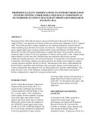
In the course of the development, our specific objectives include: (i) Establish interfaces between all key 

analysis software tools of the preliminary software system (see Fig 1) and (ii) Validate the proposed 

software system by a feasibility study on a selected RLV configuration (e.g., X-34). In what follows, we 

will discuss the total integration program architecture, the central MDO methodology ASTROS and down 

to each disciplinary domains with separate case validations. Emphasis is placed on the recent 

development of a) temperature mapping capability from aerodynamic to structural grids and b) an 

automated TPS optimization scheme using MINIVER [11]. 

2

Weight 

Model 

8 

Trajectory 

Analysis 

5 

• Mission 

Requirement • Minimum Fuel 

• Aerodynamic 

• Propulsion 

• Re-entry 

• Exo-atmosphere 

Force & 

Moment 

Database 

• Mass 

• Orbital Transfer 

(POST) 

(POST) 

• Mach Number, 

Altitude and 

Angle of Attack 

Time History 

• Parametric Geometry 

Aerodynamic Model 

Mesh Generator 

ZONAIR Unified Hypersonic 

Aerodynamics 

• Mach Number List 

• Angle of Attack List 

• Control Surface Deflection List 

• Aerodynamic 

Pressure 

C f Distribution 

Database 

Aerothermodynamic 2 

Analysis 

• Compressible Boundary Layer 

• Aero-Heating 

• Provide q, C f , C h 

(S/HABP) 

(S/HABP) 

• Temperature 

Distribution 

Database 

• Temperature C h and q 

Time History on OML 

3 

6 

Aerothermoelastic Optimization 

1 

• AIC 

FEM Model 

Mesh Generator 

ASTROS* Structural Optimization 

• Trim Analysis for Flight Loads 

• Ply thickness as design 

variables 

• Closed-Loop System Using 

ASE Module 

• Strength, Flutter and Divergent 

Constraints 

• Trim 

Solutions of 

Trajectory • Shear 

Loads 

• Shock 

Loads 

TPS Sizing 

• TPS Mass & 

Stiffness 

• Material Property 

Degradations 

• Temperature on 

Load-Carry 

Structures 

• Heat Transfer Analysis 

• TPS Design Concept 

• Stress Analysis 

7 

(MINIVER, (MINIVER, SINDA, SINDA, ASTROS*) 

ASTROS*) 

Fig 1 Block Diagram of Integrated Hypersonic Aerothermoelastic Program Architecture 

ZONAIR for Expedient Hypersonic Aerodynamics 

For the defined comprehensive multidisciplinary design/analysis optimization (MDO) development 

involving aerothermodynamics, we propose the ZONAIR code for expedient hypersonic aerodynamic 

methodology [10]. ZONAIR is a high-fidelity unstructured panel code that is unified in subsonic, sonic, 

supersonic and hypersonic Mach numbers. Given flight conditions, ZONAIR, will provide aerodynamic 

pressures/forces/magnitudes generator to efficiently create aerodynamic and loads databases for 6DOF 

simulation and critical loads identification. ZONAIR is formulated based on the unstructured surface 

panel scheme that is compatible to the finite element methods. This enables the direct adoption of offthe-shelf 

finite element pre- and post-processors such as PATRAN, I-DEAS, FEMAP, etc. for ZONAIR 

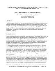
panel model generation (see Figure 2). The specific capabilities of ZONAIR include: 

• A unified high-order subsonic/supersonic/hypersonic panel methodology as the underlying 

aerodynamic force generator. 

• Unstructured surface panel scheme compatible to the finite element method. 

• Direct adoption of off-the-shelf FEM pre- and post-processors for rapid panel model generation. 

• High quality streamline solution with a hypersonic boundary layer method for aerothermodynamics. 

• Vortex roll-up scheme for high angle-of-attack aerodynamics. 

• Trim module for flexible loads and aeroheating module for aeroheating analysis. 

• Pressure interpolation scheme for transonic flexible loads generation. 

• Aerodynamic and loads database for 6 d.o.f. simulation and critical loads identification. 

ZONAIR consists of many submodules for various disciplines that include (1) AIC matrix generation 

module, (2) 3-D spline module, (3) Trim module, (4) Aeroheating module, (5) Vortex roll-up module and 

(6) Aerodynamic stability derivative module. The interrelationship of ZONAIR with other engineering 

software systems such as the pre-processor, structural finite element method (FEM), Computational Fluid 

4 

3 

• Total 

Mass 

Back to Trajectory

Dynamic (CFD) method, six degree-of-freedom (6 d.o.f.) and critical loads identification is depicted as 

follows. 

CAD 

Off-the-shelf 

pre-processor 

•PATRAN 

•I-DEAS 

•FEMAP 

•… 

Automated Automated mesh mesh generation 

generation 

AML 

AML 

ZONAIR Panel Model 

FEM solution 

3-D Spline 

AIC 

generation 

Aeroheating 

4 

ZONAIR 

Trim 

analysis 

Aerodynamic 

force/ moment 

generation 

Pressure 

interpolation 

CFD/Windtunnel 

pressures 

Aerodynamic 

and loads 

database 

Fig 2 ZONAIR and It’s Interfacing Capacity with Other FEM Software 

6 d.o.f. 

simulation 

Critical loads 

identification 

ZONAIR has been under continuous development by ZONA throughout the last decade. ZONAIR’s 

current version has proven capability accounting for multi-body interference, ground interference, wave 

reflection and store-separation, aerodynamics in hypersonic/supersonic as well as subsonic flow domains 

(Table 1). By comparison, ZONAIR is clearly the best choice as an expedient and versatile aerodynamic 

methodology. In what follows, we present the ZSTREAM development along with the hypersonic 

aerodynamics/aerothermodynamics applications based on ZONAIR whose results are compared with that 

of CFL3D [12]. These include: 

− CKEM(Compact Kinetic Energy Missile) at M = 6.0, α = ± 2° 

− 15° Blunt Cone at M = 10.6 and α = 5° 

− X-34 at M = 6.0, α = 9° and altitude = 183 Kft 

Finally, a TPS sizing example employing heat rate input provided by ZONAIR + SHABP [13] from its 

coupled trajectory/aeroheating solution, is presented. 

Code Method Comp. 

Eff. (X- 

34) 

Table 1. Comparison of Various Aerodynamic Codes. 

Grid 

Gen. 

Subsonic/ 

Supersonic/ 

Hypersonic 

Multi 

Body 

Interf 

Ground 

Effect 

Aeroheating 

Geo. 

High 

Fidelity 

6 DOF 

Store 

Sep. 

Aeroload 

at FEM 

GRID 

CFL3D Euler/NS 30 hrs Needed All Yes Yes Yes Yes No No 

ZONAIR Potential 

+ 

Perturbed 

Euler 

20 min No All Yes Yes Yes Yes Yes Yes 

APAS Potential

compressibility stretch in the axial direction. A local pulsating body analogy has been established to 

account for shock/flow rotationally effects. ZONAIR is found to yield excellent trends following those of 

Exact Euler steady/unsteady solutions (Sims and Brong) in terms of static and dynamic stability 

derivatives throughout all Mach numbers from shock detachment to Mach 20. Expedient and accurate 

predictability in stability derivatives is one of the superior features of ZONAIR. A detailed theoretical 

formulation of ZONAIR is found in [4, 10]. 

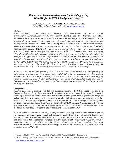
Fig 3 shows the ZONAIR pressure distribution and aerodynamic force/moments along the CKEM body at 

M=6.0 for various bent-nose angles and angles of attack and compared with CFL3D results. In all cases, 

the ZONAIR results agree very well with those of CFL3D. Note that CFL3D requires over 2 hours of 

computer time for each bent-nose case whereas ZONAIR takes only 1 minute. 

C P 

C P 

Undeflected Case, Body & Nose at the same AOA 

(Nose = Body = -2°, at M=6.0) 

0.2 

0.18 

0.16 

0.14 

0.12 

0.1 

0.08 

0.06 

0.04 

0.02 

0 

M = 6.0 -2° 

-2° 

Cp_lower CFL3D 

Cp_upper CFL3D 

Cp_lower ZONAIR 

Cp_upper ZONAIR 

-0.02 

0 5 10 15 20 

x 

25 30 35 40 

0.2 

0.18 

0.16 

0.14 

0.12 

0.1 

0.08 

0.06 

0.04 

0.02 

0 

5 

Positive 2° Deflection between Body & Nose 

(Nose = 0°, Body = -2°, at M=6.0) 

CFL3D ZONAIR 

0.16 

0.14 



CFL3D ZONAIR 

0.12 


CL -0.118 -0.1125 0.1 

Cp_upper ZONAIR CL -0.076 -0.0712 

0.06 

Cm -0.0549 -0.05588 Cm -0.02552 -0.02776 

0.04 

CD 0.0465 0.050 0 

CD 0.0553 0.049 

Ch -0.00612 -0.00668 


(Nose = 2°, Body = 0°, at M=6.0) 

M = 6.0 

2° 





-0.02 

0 5 10 15 20 

x 

25 30 35 40 

C P 

0.08 

0.02 

-0.02 

M = 6.0 

-2° 

-0.04 

0 5 10 15 20 

x 

25 30 35 40 

Ch 3.76e-7 0 


(Nose = 4°, Body = 2°, at M=6.0) 

CFL3D ZONAIR Cp_lower CFL3D 

CFL3D ZONAIR 


0.2 


CL 0.0437 0.0408 CL 0.1637 0.1517 

0.16 

0.12 

Cm 0.0292 0.02806 

0.08 

2° 

Cm 0.0857 0.08388 

0.04 

CD 0.0492 0.0493 

0 

CD 0.0537 0.057 

Ch 0.00612 0.00668 

lift force , drag force , pitch moment about C.G. , 

CL 

= CD 

= 

Cm 

= 

Ch 

= 

q∞ 

AB 

q∞ 

AB 

q∞ 

AB 

L 

C P 

0.28 

0.24 

M = 6.0 4° 


-0.04 

0 5 10 15 20 

x 

25 30 35 40 

moment of nose section about x = 7 ′′ 

q∞ 

AB 

L 

Ch 0.0123 0.0133 

hinge , AB = 2.405 in 2 , L = 40.25 in 

Fig 3 ZONAIR Pressure Distributions and Aerodynamic Force/Moments along the CKEM Body 

at M = 6.0 for Various Bent-Nose Angles and Angles of Attack 

ZSTREAM for Robust Streamline Computation 

The development of ZSTREAM was prompted by the breakdown of QUADSTREAM in SHABP [13] at 

the stagnation points and its independency of freestream mach numbers. ZSTREAM is a finite element 

based streamline code, which is Mach number dependent and uniformly valid everywhere on the body 

surface. It is capable to define/plot high quality streamline solutions in the complete flow domain on the 

body surface, including the stagnation point, according to surface flow solutions given by a panel code 

(for example, ZONAIR) or a CFD code (For example, CFL3D). These streamline solutions of the CKEM 

body, the 15º blunt cone and X-34 are shown in Fig 4. ZSTREAM functionality is to provide streamlines 

input for Aeroheating/Heat-transfer programs such as SHABP for computations of the heat-transfer rate at 

the body surface.

(a) 

(b) 

(c) 

Fig 4 Streamline Results of (a) CKEM at M=6.0 and α=2°, 

(b) 15° Blunt Cone at M=10.6 and α=5°, (c) X-34 at M=6 and α=9° 

Aerothermodynamic Analysis by ZONAIR 

To validate the ZONAIR/ZSTREAM/SHABP procedure, we have performed the aeroheating analysis on 

three configurations, namely the CKEM body (Figs 5 and 6), a 15° blunt cone (Figs 7 and 8) and the 

simplified X-34 wing-body configuration (Figs 9 and 10). Note that the hypersonic boundary layer 

method in SHABP is developed based on the similarity solutions of compressible (laminar/turbulent) 

boundary layer methodology of Eckert/Boeing Rho-Mu, Spalding-Chi, and the White-Christoph methods 

[15]. The aeroheating results using the ZONAIR+ZSTREAM+boundary layer approach are validated 

with the CFL3D/Euler+LATCH [16] results on all cases considered. Good correlations on the inviscid 

Cp, heat transfer rates and surface temperature distributions can be seen from Figs 5-10. 

It should be noted that the streamline computation procedure of LATCH is based on an integral method 

that contains a singularity at the stagnation point. This singularity prohibits the graphic capability of 

LATCH in the neighborhood of the nose, hence the cut out (Figs 6a, 8a). By contrast, ZONAIR is free 

from such singularity prohibition because of its finite element-based streamline procedure of ZSTREAM. 

0.15 

0.14 

0.13 

0.12 

0.11 

0.1 

0.09 

0.08 

0.07 

0.06 

0.05 

0.04 

0.03 

0.02 

0.01 

0 

CKEM Body: M = 6.0, α = 2û 

ZONAIR CFL3D/Euler 

0.15 

0.14 

0.13 

0.12 

0.11 

0.1 

0.09 

0.08 

0.07 

0.06 

0.05 

0.04 

0.03 

0.02 

0.01 

0 

(a) Inviscid Surface Pressure 

6 

Cp 

0.12 

0.1 

0.08 

0.06 

0.04 

0.02 

0 

CFL3D 

ZONAIR ZONA7U 

-0.02 

0 5 10 15 20 

x (in.) 

25 30 35 40 

(b) Wind-Side Inviscid Surface Pressure (φ=180º) 

Fig 5 Inviscid Surface Pressure on CKEM at ∞ M =6.0, α=2°, ∞ p =2.66 lb/ft2 , T ∞ =89.971ºR, T w =540ºR

1.8 

1.64 

1.48 

1.32 

1.16 

1 

0.84 

0.68 

0.52 

0.36 

0.2 

0 04 

0.45 

0.43 

0.41 

0.39 

0.37 

0.35 

0.33 

0.31 

0.29 

0.27 

0.25 

0.23 

0.21 

0.19 

0.17 

0.15 

0.13 

0.11 

0.09 

0.07 

0.05 

ZONAIR CFL3D/Euler + LATCH 

0.45 

0.43 

0.41 

0.39 

0.37 

0.35 

0.33 

0.31 

0.29 

0.27 

0.25 

0.23 

0.21 

0.19 

0.17 

0.15 

0.13 

0.11 

0.09 

0.07 

0.05 

(a) Laminar Heat Transfer Rates (Btu/ft 2 (b) Wind-Side Laminar Heat Transfer Rates (φ=180º) 

-s) 

Fig 6. Laminar Heat Transfer Rates on CKEM at ∞ M =6, α=2°, ∞ p =2.66 lb/ft2 , T ∞ =89.971ºR, T w =540°R. 

15û Blunt Cone: M = 10.6, α = 5û 

ZONAIR CFL3D/Euler 

1.8 

1.64 

1.48 

1.32 

1.16 

1 

0.84 

0.68 

0.52 

0.36 

0.2 

0 04 

7 

qdot (Btu/ft 2 -s) 

0.4 

0.3 

Cp 0.2 

0.1 

0.28 

0.24 

0.2 

0.16 

0.12 

0.08 

0.04 

CFL3D+LATCH 

ZONAIR 

0 

0 10 20 

x (in.) 

30 40 

Test 

CFL3D 

ZONAIR ZONA7U 

0 

0 2 4 6 8 10 12 14 16 18 

x (in.) 

(a) Inviscid Surface Pressure (b) Wind-Side Invisicid Surface Pressure (φ=180º) 

Fig 7. Inviscid Surface Pressure on a 15° Blunt Cone at M∞=10.6, α=5°, p ∞ =2.66 lb/ft 2 , T ∞ =89.971ºR, T w =540ºR 

12 

11 

10 

9 

8 

7 

6 

5 

4 

3 

2 

1 

0 

“Cut-out” due to 

singularity at 

stagnation point 

ZONAIR CFL3D/Euler + 

LATCH 

12 

11 

10 

9 

8 

7 

6 

5 

4 

3 

2 

1 

0 

“Cut-out” 

due to 

singularity 

at stagnation 

point 

qdot (Btu/ft) 

10 

8 

s) 

d 6 

t 

Bt 

/f 

4 

2 

Test 

CFL3D+LATCH 

ZONA7U+SHABP 

ZONAIR 

0 

0 2 4 6 8 10 12 14 16 18 

x (in.) 

(a) Laminar Heat Transfer Rates (Btu/ft 2 -s) (b) Wind-Side Laminar Heat Transfer Rates (φ=180º) 

Fig 8. Laminar Heat Transfer Rates (Btu/ft 2 -s) on 5º Blunt Cone at 

M∞=10.6, α=5°, p ∞ =2.66 lb/ft 2 , T ∞ =89.971ºR, T w =540ºR.

-0.04 0.12 0.28 0.44 0.6 0.76 0.92 1.08 1.24 1.4 1.56 

ZONAIR CFL3D 

(a) Front View 

8 

-0.04 0.12 0.28 0.44 0.6 0.76 0.92 1.08 1.24 1.4 1.56 

-0.04 0.12 0.28 0.44 0.6 0.76 0.92 1.08 1.24 1.4 1.56 -0.04 0.08 0.2 0.32 0.44 0.56 0.68 0.8 0.92 1.04 1.16 1.28 1.4 1.52 1.64 

(b) Wind-Side 

-0.04 0.12 0.28 0.44 0.6 0.76 0.92 1.08 1.24 1.4 1.56 

-0.04 0.08 0.2 0.32 0.44 0.56 0.68 0.8 0.92 1.04 1.16 1.28 1.4 1.52 1.64 

(c) Lee-Side 

Fig 9. Inviscid Surface Pressure Distributions on the X-34 at M∞=6, α=9°; 

(a) Front View, (b) Wind-Side, and (c) Lee-Side. 

300 500 700 900 1100 1300 1500 1700 

1500 

1200 

900 

600 

300 

ZONAIR 

(a) Front View 

1800 

1700 

1600 

1500 

1400 

1300 

1200 

1100 

1800 

1700 

1600 

1500 

1400 

1300 

1200 

1100 

(b) Wind-Side 

CFL3D+LATCH 

“Cut-out” due to 

singularity at 

stagnation point 

300 500 700 900 1100 1300 1500 1700 

(c) Lee-Side 

Fig 10. Turbulent Surface Temperatures (°F) on the X-34 at M∞=6, α=9°, 

Alt.=183 Kft; (a) Front View, (b) Wind-Side, and (c) Lee-Side. 

Trajectory Analysis 

The main function of the trajectory analysis is to obtain an optimal trajectory that minimizes the fuel 

while satisfying other constraints such as Mach number needed for specific engine usage, final velocities, 

altitudes, launch angle, etc. 

1500 

1200 

900 

600 

300

Here, ZONAIR + SHABP is used to compute the heat rate at the stagnation point of the X-34 according 

to two assigned trajectories (X1004601 and X1004701). Good correlation is found between the present 

ZONAIR + SHABP method and MINIVER [11] (Fig 11). 

ZONAIR + SHABP only requires the trajectory inputs to be submitted once, then it outputs the pressure 

(Cp, not shown) and the heat-rate ( q! ) solutions. For 14 time steps along a stretch of 800 seconds of the 

flying time, it requires less than 10 minutes of computing time. By contrast, MINIVER requires manual 

input for each point of interest; i.e., each output q! curve requires approximately 5 to 10 minutes. 

Heat Rate (Btu/ft 2 Heat Rate (Btu/ft -s) 

2 -s) 

Heat Rate (Btu/ft 2 Heat Rate (Btu/ft -s) 

2 -s) 

10 

8 

6 

4 

2 

Miniver 

ZONA7U ZONAIR + 

SHABP 

0 

0 200 400 600 800 

Time (s) 

(a) 

10 

8 

6 

4 

2 

Miniver 

ZONA7U ZONAIR + 

SHABP 

9 

altitude (Kft) 

angle of attack (deg.) 

Ma 

300 

250 

200 

150 

100 

50 

0 

40 

30 

20 

10 

(a) 

(b) 

0 500 1000 1500 

time (s) 

(a) 

(b) 

0 

0 500 1000 1500 

time (s) 

10 

8 

(a) 

6 

4 

2 

0 

(b) 

0 500 1000 1500 

time (s) 

0 

0 200 400 600 800 

Time (s) 

(b) 

(c) 

Fig 11. Heat Rate Comparison at Stagnation Point 

(a) X1004601, (b) X1004701, (c) Trajectory and flight condition history. 

TPS Sizing and Optimization 

The TPS sizing procedure 

The TPS sizing objective is to develop a procedure to minimize the TPS weight while satisfying the 

thermal protection requirement and the load-carrying requirement of the combined RLV/TPS structure. 

The developed TPS sizing procedure can be demonstrated by a constructed prototypical TPS/AFRSI 

(Advanced Flexible Reusable Surface Insulation) model [17]. (Fig 12)

heat rate (Btu/ft^2-s) 

q! q! q! 

Layer Layer 1 1 - - Coating Coating (h (h o = 0.01 in. HRSI Coating) 

Layer 2 - Outer Fabric (h o = 0.015 in. Outer Fabric AB312) 

Layer (3) Insulation 

a. Q-Felt Insulation (standard) 

b. Q-Felt 3.5PCF x (inches) 

c. 6LB Dynaflex 

(h o = 1.2 in) 

Layer 4 - Inner Fabric (h o = 0.009 in. Inner Fabric AB312) 

Layer 5 - Adhesive (h o = 0.008 in. RTV Adhesive) 

Layer 6 - Structure (h o = 0.011 in. Aluminum) 

• h o is the initial thickness 

• T outer and T interior are the temperatures at the outer edge and (1) to (5) interior layers of the TPS. 

T skin is the temperature at the nodes within the skin layer 6. 

2 

1 

Fig 12. Description of the model TPS system (AFRSI from NASA TM 2000-210289 [17]). 

0 

0 200 400 

time (s) 

600 800 

Point A 

L 

Fig 13. Location and Heat Flux History to Evaluate TPS Size on Windward Side of X-34 Centerline 

(bottom view and side view, L=50 in.) Heat Flux is Based on Trajectory X1004601. 

With this model, the objective becomes one to minimize the total weight of a TPS system as such. The 

inequality constraints are the maximum allowable operating temperature of each layer (characterized by 

the layer material) including that of the skin layer (Fig 12), whereas the thickness of each layer is the 

design variable. A typical TPS element, as an “elementary TPS system” is selected on the windward 

centerline of X-34 (Fig 13). The model input is the heat rate, q! , which is currently provided by 

ZONAIR+SHABP through the trajectory aerothermodynamic prediction (Fig 14). Maximum 

temperatures in each layer, layer thickness and the total minimum TPS weight are resulting outputs, 

obtained by applying the following optimization procedure to MINIVER/EXITS (Table 2). The 

developed code is called MINIVER/OPT. 

10

heat rate (Btu/ft^2-s) 

2 

1 

Input 

Heat Flux History 

0 

0 200 400 

time (s) 

600 800 

h 

1 

h 

2 

h 

n 

TPS Sizing 

11 

Temperature (F) 

Fig 14 Input/Output of TPS Sizing 

Layer 1 

Layer 2 

Layer n 

T o 

. 

q 

Fig 15 Typical TPS sizing problem 

800 

600 

400 

200 

Output 

Max Max Touter 

T outer 

Max Max Tinterior 

T interior 

Max Max Tskin 

T skin 

0 

0 200 400 600 800 1000 

time (s) 

Fig 15 depicts a typical TPS design problem, which consists of n layers of different TPS materials. This 

design process can be automated by formulating an optimization problem statement as follows 

n 

Minimize : W = ∑ ρ h 

i= 

1 

i i 

Subject to : T i < T , i = 1, 2 … n (1) 

oi 

Design variable : h i ≥ h , i = 1, 2 … n 

max i 

where W is the total weight of the TPS system to be minimized, 

ρ i is the density of the ith layer, 

T i is the temperature in the ith layer, 

T oi is the maximum operation temperature of ith layer’s material, 

h i is the thickness of the ith layer, 

and h maxi is the side constraint of the ith layer. 

This optimization problem can be solved by linking a TPS analysis code such as MINIVER/EXITS [11] 

module with an optimization driver like the usable/feasible direction method imbedded in ASTROS [5]. 

One of the essential elements in the usable/feasible direction method is the sensitivity of the temperature 

time history of each layer with respect to the design variable h . i 

Many techniques, such as Finite Difference Method (FDM), Automatic Differentiation (ADIFOR), 

Symbolic Differentiation, the Complex Variable Differentiation (CVD) technique, can be adopted and 

applied to the MINIVER/EXITS module to provide sensitivity. Among them, the CVD technique is 

x

selected because by comparison it is a “numerically-exact” method and requires the least programming 

effort. 

The Complex Variable Differentiation (CVD) technique was first originated by Lyness and Moler [18]. 

In the complex variable approach, the variable x of a real function f (x) 

is replaced by a complex one, 

x + i∆ h. 

For small ∆ h , f(x+ i∆ h) can be expanded into a Taylor’s series as follows: 

2 2 3 3 4 4 

df ∆h d f ∆h d f ∆h 

d f 

f ( x + i∆ h) = f ( x) + i∆h − − i + ... 

(2) 

dx 2 2 6 3 24 4 

dx dx dx 

The first and second derivatives of the above equation can be expressed as: 

( + ∆ ) 

12 

2 ( ) 

df Im ⎡fxih⎤ = 

⎣ ⎦ 

+ O ∆h 

dx ∆h 

( ) 

( ) − ( + ∆ ) 

2 

d f 2 ⎡f x Re f x i h ⎤ 

= 

⎣ ⎦ 

+ O ∆h 

2 2 

dx ∆h 

2 ( ) 

where the symbol “Im” and “Re” denote the imaginary and real parts, respectively. From Eqs. (3) and 

(4), it can be seen that the derivatives using the CV approach only require function evaluations. This 

feature is very attractive particularly when the function is sufficiently complicated, in which case to 

obtain an analytic derivative is cumbersome and error-prone. Unlike the finite difference method, where 

the accuracy of the derivative depends on the step-size, Eq. (3) shows that the first derivative does not 

involve differencing two functions followed by magnification of the subtraction error (because of the 

division by the step size ∆ h ). In fact, no cancellation errors exits for the first derivative in the CVD 

technique, thus the first derivative is step-size independent. Note that the second derivative in Eq. (4) is 

prone to cancellation errors (because of the subtraction of two close numbers), but is not used here. 

Because CVD does not introduce cancellation (roundoff) error for the first derivative, the step-size ∆ h 

30 

can be chosen as small as the machine zero, e.g., 10 − 

∆h = . Hence, the truncation error due to Taylor’s 

2 60 

series of the order of 10 − 

∆h = that approaches to essentially a machine zero in a 32 bit computer. 

For first derivative, CVD does not seem to introduce any approximation in its numerical differentiation, 

rather it is a nearly “numerically-exact” differentiation technique. 

To incorporate CVD into the MINIVER/EXTIS module (called MINIVER/OPT) for sensitivity is rather 

straightforward. One can simply declare all variables in the code as complex variable and introduce a 

30 

small imaginary perturbation ( 10 − 

i ∆h = i × ) in the design variable h i . Division of the imaginary part 

of the temperature time history in each layer by ∆ h yields the sensitivity. 

To validate the accuracy of the sensitivity MINIVER/OPT, we select the constructed prototypical TPS 

system using an AFRSI (Advanced Flexible Reusable Surface Insulation) module, Fig. 12. 

With the given heat/flux . 

q at point A (depicted in Fig 13) we focus on the temperature sensitivity of layer 

6. The sensitivity ∂T6 

, which precisely corresponds to the temperature change at the aluminum 

∂h 

3 

structure due to the thickness perturbation of the Q-Felt insulation material (layer No. 3), computed by 

MINIVER/OPT is shown in Figure 16. The negative values of the sensitivity indicate the decrease of 

(3) 

(4)

temperature due to the increase of thickness; as expected. Comparing to the results of CVD, the relative 

error of the sensitivity computed by FDM with various step size is depicted in Fig 17. It can be seen that 

the error of FDM decreases while the step size decreasing. But with a very small step size ( − 8 

∆ h = 10 ), 

the error increases, showing that the accuracy of FDM is step-size dependent. 

∂T6 

0 

-20 

∂h3 

-40 

-60 

-80 

complex variable differentiation, ∆h3 = e-30 

0 200 400 600 800 1000 

time (sec) 

Fig 16 Sensitivity ∂T6 ∂ h3 

by MINIVER/OPT in the entire history 

Error % 

0.001 

0.0001 

0.00001 

relative error of sensitivity at layer 6 (FD - CV)/CV 

100 

10 

1 

0.1 

0.01 

8 

10 − 

∆h = 

0 200 400 600 800 1000 (sec) 

13 

2 

10 − 

∆h = 

3 

10 − 

∆h = 

4 

10 − 

∆h = 

6 

10 − 

∆h = 

Fig 17 Relative error of FDM and CVD for sensitivity ∂T6 ∂ 

h3

weight (lbm/ft^2) 

weight (lbm/ft^2) 

1.2 

1 

0.8 

0.6 

0.4 

0.2 

0 

1.2 

1 

0.8 

0.6 

0.4 

0.2 

0 

0 1 2 3 4 

optimizaton cycle 

(a) Case A with a given q! (in 263 Sec) 

0 2 4 6 8 

optimization cycle 

(b) Case B with 1.5x q! (in 396 Sec) 

Figure 18 Weight variation of the modeled TPS System (AFRSI) during optimization 

Tstr (F) 

500 

400 

300 

200 

100 

0 

Temperature History at Structure Layer 

0 200 400 600 800 1000 

Time (sec) 

14 

initial (W = 0.777 

lbm/ft^2) 

5th cycle (W = 0.590 

lbm/ft^2) 

final (W = 0.668 

lbm/ft^2) 

Fig 19 Case B Temperature history at the structure layer (Layer 6) during optimization process

Table 2 Case A Optimization Results 

Specific 

heat 

(But/lbm° 

F) 

15 

Initial 

thick- 

ness 

(in) 

T max 

in 

layer 

Layer 

Material and 

Temp limit (°F) 

density 

(lbm/ft 3 ) 

(°F) 

Optimized 

thickness 

(in) 

1 HRSI Coating 

2300 

104 0.20 0.01 705.2 0.0072 

2 AB312 Fabric 

2024 

61.5 0.166 0.015 704.9 0.0072 

3 Q-Felt 

1800 

3.5 0.1875 1.2 701.6 0.66849 


2024 

61.5 0.166 0.009 300.0 0.0072 

5 RTV-560 

550 

88 0.285 0.008 300.0 0.0072 

6 Aluminum 

300 

173 0.22 0.011 300.0 0.011 

- Layer Thickness: upper bound 1.0”, lower bound 0.0072” 

- Given Input heat flux q! , see Fig 13 

- Optimized Weights Winitial = 0.777 lbm/ft 2 , Wfinal = 0.543 lbm/ft 2 

Shown in Table 2 is the optimization results of the AFRSI TPS system depicted in Figures 12 and 13 

(Case A). In this optimization problem, the thickness of first five layers are defined as design variables 

with initial thickness and maximum operational temperature shown in Table 2. The upper bound and 

lower bound of these five design variables are assumed to be 1.0” and 0.0072”, respectively. The 

thickness of aluminum layer (layer 6) remains unchanged because it represents the load-carry structure 

and is not a part of the TPS system. It can be seen that all design variables reach the lower bound 

(0.0072”) except the Q-Felt layer. This is expected because the Q-Felt layer has the lowest density and 

thermal conductivity that provide the highest thermal insulation capability with least structural weight. 

Table 3 Case B Optimization Results 

Specific 

heat 

(But/lbm° 

F) 

Initial 

thick- 

ness 

(in) 

T max 

in 

layer 

Layer 

Material and 

Temp limit (°F) 

density 

(lbm/ft 3 ) 

(°F) 

Optimized 

thickness 

(in) 

1 HRSI Coating 

2300 

104 0.20 0.01 814.5 0.0072 


2024 

61.5 0.166 0.015 814.3 0.0072 

3 Q-Felt 

1800 

3.5 0.1875 1.2 810.0 0.6000 


2024 

61.5 0.166 0.009 300.0 0.0072 

5 RTV-560 

550 

88 0.285 0.008 300.0 0.02705 

6 Aluminum 

300 

173 0.22 0.011 300.0 0.011 

- Layer Thickness: upper bound 0.6”, lower bound 0.0072” 

- Given Input heat flux 1.5x q! , see Fig 13 

- Optimized Weights Winitial = 0.777 lbm/ft 2 , Wfinal = 0.668 lbm/ft 2

Table 3 presents the optimization results of the same AFRSI TPS system but with a magnified heat flux 

(by a factor of 1.5) and a reduced upper bound in design thickness (Case B). The optimized result is that 

the thickness of the Q-Felt layer reaches the upper bound and that of the RTV-560 layer become 0.02705” 

while the thickness of other layers remain at the lower bound. This indicates that because of the higher 

heat flux input, the Q-Felt layer with the upper bound thickness alone is not sufficient to satisfy the 

temperature constraints at all layers. Other than the Q-Felt layer, the next best thermal protection material 

is the RTV-560 layer because of its highest value of specific heat ( c p ). Although, the RTV-560 layer has 

a high density ρ which may not be structurally efficient, however, its higher ρ cp 

value can offer a good 

thermal protection capability. Indeed, MINIVER/OPT can detect this capability and thereby increase the 

thickness of the RTV-560 layer from the lower bound to 0.02705”. 

Figures 18 presents the weight variance versus design cycles during the optimization process. Note that 

case A the nominal heat-flux achieves optimized weight with 3 cycles in 4.5 minutes; whereas case B 

(with 1.5 times heat-flux) takes 8 design cycles in 6.5 minutes. 

Figure 19 presents the time history of the temperature of Case B of the aluminum layer during its eight 

optimization design cycles. With the maximum operational temperature being 300°F of the aluminum as 

one of the design constraints, it can be seen that the initial thickness is over-designed because its 

maximum temperature is only approximately 230°F. Meanwhile, an intermediate design offers a least 

weight but its maximum temperature (400°F) violates the constraint. The maximum temperature of the 

final design is exactly 300°F, indicating that it is an optimum design. 

Smart Structures Module 

Modeling of PZT and SMA 

activations and computes 

the induced aerodynamic 

control forces. 

ZAERO Aerodynamic 

Module 

Unified steady/unsteady 

aerodynamics for subsonic, 

transonic, supersonic, and 

hypersonic flows. 

Sensitivity Analysis 

Provides sensitivity of 

stresses, stability, and 

performance with 

respect to structural 

design variables. 

Smart structures module 

electrodes 

3 

piezoelectri c 

voltage 

2 

ZAERO/UAIC 

1 

UNSTEADY AERODYNAMICS 

Structural Finite Element Module 

NASTRAN-compatible FEM analysis 

ASE 

ZAERO 

Bas e lin e FE 

Str u ct ur al 

UA IC Mo du l e 

M odel 

Va ri at ions 

ASE Module 

Ge ne ra li ze d 

Ma tr ic es 

Co n tr ol 

R at iona l Aer o dyn ami c 

Gu st 

Mo de 

Approx ima ti on s 

M odel 

Sta te S p ac e 

ASE Model 

Ope n / 

Co n tr ol 

Gu st 

Ma rg i ns 

Close d -l oop 

Res p onse 

Fl ut te r 

An al ys is 

Re sult s 

Sens iti v ity 

Ana lysis 

16 

Trim module 

ASE Module 

State-space aeroservoelastic analysis including SISO/MIMO 

control system for stability and gust loads analysis. 

Fig 20 Engineering Modules in ASTROS* 

Trim Module 

Static aeroelastic 

analysis for flight 

loads and optimum 

trim solutions 

Aeroelastic Stability 

Module 

Provides true damping 

flutter solutions. 

Optimization Module 

An optimizer driving all 

modules to achieve the 

optimum design. 

TRIM Analysis using ASTROS* and ZONAIR 

ASTROS* is an enhanced version of ASTROS (Automated Structural Optimization System [5]), an 

internationally acclaimed MDO software developed by Northrop Grumman Corporation for the Air 

Force. Under a two-year contractual support by AFRL, ZONA has further enhanced ASTROS by 

seamlessly integrating several engineering modules into ASTROS [19, 20]. Fig 20 depicts all the 

essential modules of ASTROS*, including a unified aerodynamic module (ZAERO), a NASTRAN-based

structural finite element module, a smart structure module, a trim module, an aeroelastric stability 

module, an aeroservoelastic module, a sensitivity analysis module, and an optimization module. 

The trim analysis for the flexible X-34 is performed using ASTROS* in conjunction with ZONAIR to 

account for the static aeroelastic effect of the vehicle. The outcomes of the trim analysis are the control 

surface deflection angles, load factors, etc. as well as the stress distribution in the structures. Fig 21 

depicts an ASTROS* finite element model of the X-34 that includes the modeling of the TPS mass and 

the material property degradations on the load carrying structure due to aeroheating effects as computed 

by ZONAIR. The ASTROS* trim analysis shows that in order to trim the X-34 at M = 6.0, α = 9° and 

altitude = 183 Kft, the required trailing edge flap angle is 2.05° degrees and a load factor of 0.97-g for a 

total weight of 16,000 lbs. At this condition, the aerodynamic loads computed at the ZONAIR panels are 

then mapped to the FEM grid using the 3D spline module; allowing a subsequent stress analysis of the 

structures. Such a stress distribution is shown in Fig 22. 

Fig 21 X-34 Finite Element Model 

Fig 22 X-34 Stress Distribution at M=6.0, α=9°, Alt=183 Kft 

Temperature Mapping for Aerothermoelastic Analysis 

• Temperature and Aeroloads Mapping from Aerodynamic to Structural Grids 

For the present aerothermoelastic analysis, two types of data mapping between the aerodynamic grid (the 

aerodynamic panels) and the structural finite element (FEM) grid are required. The first type is the 

mapping of the aerodynamic forces from the aerodynamic grid to the structural grid as well as the 

displacement from the FRM grid back to the aerodynamic grid. This type of data mapping procedure has 

been fully developed in ASTROS*, and has been applied to the previous ZONAIR/TRIM analysis for the 

force mapping. The second type of mapping is one that transfers the temperature distribution on the skin 

of RLV to that on the outmost structural surface. Note that this is strictly a grid system mapping for 

temperature transferal whereas no heat transfer is assumed to take place. In terms of finite element 

context, this amounts to the mapping of the temperatures (of the TPS skin layer) from the ZONAIR 

surface grid to the outmost FEM grid. 

Since, FEM elements/grids are filled within and extended to the surface of the RLV it is required to 

identify the outmost FEM surface compatible with the ZONAIR surface for temperature mapping. As 

these two surfaces are likely to be misaligned, then a projection scheme is required to perform the 

temperature mapping “outward” or “inward” from the ZONAIR surface grids. 

The second type mapping requirement is the temperature mapping from the aerodynamic grid to the FEM 

surface grid. There are two technical challenges involved in the development of such a mapping 

procedure: 

17

(1) Because the FEM model contains elements/grids on the surface skin as well as the internal 

structures, it is required to identify those only on the surface skin for temperature mapping. 

(2) Because the wet surface skin defined by the ZONAIR mesh and FEM surface mesh may have 

discrepancy, the temperature mapping requires a projection procedure that can either project 

“outward” or “inward” from the ZONAIR panels. 

• Temperature Mapping Procedure 

A finite-element procedure has been developed for temperature mapping that assumes the coordinates and 

temperatures at any point on the ZONAIR model can be determined by the nodal values of the ZONAIR 

panels through the shape functions expressed as 

( ξη) 

X N , X α 

= ∑ α 

(5) 

α 

where X is the coordinates or temperatures at any given point 

N α ( ξ , η ) is the shape functions and ξ , η are the intrinsic coordinate of the shape 

function 

α is the number of nodes of a ZONAIR panel, and 

X α is the coordinates or temperatures at ZONAIR nodes. 

For a given structural FEM grid p as shown in Figure 23, the point q on the ZONAIR model that has the 

minimum distance to p can be found by solving 

where X is the coordinates of point q 

p 

X is the coordinates of point p 

n is the out-normal of vector of the ZONAIR panel, and 

λ is a multiplication factor to n. 

p 

X − X = λn 

(6) 

A FEM grid p is a surface grid only if no FEM elements are located between the points p and q. This 

condition can be determined by solving the following equation 

( ) 

p q p 

X − X = t X − X 

(7) 

Figure 24 shows a FEM element that is located between the points p and q. The point s on the element 

q p 

which intersects the vector X − X has the conditions such that −1≤ξ≤ 1, 

−1≤η≤ 1 and −1≤ t ≤ 1, 

where t is the position tracking parameter. 

To validate the above procedure, we select the X-34 FEM model as the test case. Fig 25a depicts the X- 

34 FEM model that consists of surface skin elements as well as the elements modeling the internal 

structures. The resulting surface grid and elements are shown in Figure 25b where the removal of the 

internal structures can be clearly seen. 

Once the FEM grid is identified as a structure grid, then its temperature is assumed to be the same as that 

at the closest ZONAIR surface point. It should be noted that the temperature at any ZONAIR surface 

points can be calculated using the shape function shown below 

( ξη) 

T N , T α 

= ∑ α 

(8) 

α 

18

where T α is the temperature at the ZONAIR nodal points. 

Shown in Figure 26a and 26b is a temperature distribution computed on the X-34 ZONAIR model and the 

mapped temperature on the FEM surface grid/elements. Overall, the mapped temperature agrees well 

with the computed temperature, showing the accuracy of the developed temperature mapping 

methodology. 

ZONAIR 

panel 1 

q 

n 

ZONAIR 

panel 2 

X-X 

p 

p point on ZONAIR model 

closest to FEM gird p 

(FEM grid) 

Fig 23 Minimum distance between the FEM grid p and 

a point on the ZONAIR model q 

19 

FEM element 

X-X p 

s 

p 

Fig 24 A FEM element located between point p and q 

q 

X q -X p 

(a) X-34 full FEM model (b) X-34 surface grid/elements 

Fig 25 Removal of the internal grid and elements on the X-34 FEM model 

TEMP 

3340 

3117.29 

2894.57 

2671.86 

2449.14 

2226.43 

2003.71 

1781 

1558.29 

1335.57 

1112.86 

890.143 

667.429 

444.714 

222 

ZONAIR panel 

(a) Temperature distribution 

(b) Mapped temperature on 

computed on ZONAIR model 

FEM surface elements/grids 

Fig 26 Temperature mapping results on the X-34 FEM model 

TEMP 

3340 

3117.29 

2894.57 

2671.86 

2449.14 

2226.43 

2003.71 

1781 

1558.29 

1335.57 

1112.86 

890.143 

667.429 

444.714 

222

Automated Mesh Generation using AML 

Present ZONAIR/ASTROS integration effort directs toward a fully user-oriented 

aerothermodynamic/aerothermoelastic tool for RLV/TPS design. To this end, their integration with 

design-oriented automated mesh generation software is desirable. Prior integration of AML (adaptive 

modeling language) with SHDV (supersonic hypersonic vehicle design) system has shown the former is a 

viable user-oriented mesh generator suitable for aerospace vehicle design. Its capability to generate and 

rapidly alter design configuration is controlled by a set of essential generic geometric parameters. In fact, 

AML could manage and automate the data transfer between various design and analyses tools. [6] 

Specifically, AML can expediently generate FEM element meshes for NASTRAN as well as that for 

ASTROS, because both use the same bulk data input format. Adopted a unstructured finite-element type 

panel scheme, ZONAIR also shares a similar bulk data input format. Thus, applying AML to ZONAIR 

/ASTROS for mesh generation is a straightforward task. Our next step is to integrate ZONAIR/ASTROS 

and the other software in the aerothermodynamic/aerothermoelastic architecture (Figure 1) with AML 

into a feature-based design environment. 

Presented here are some preliminary results generated by the coupling of AML with ZONAIR 

demonstrating a 2-body RMLV design process. Figure 27 shows various views of the 2-body RMLV 

design. Figure 28 shows the automated generation of ZONAIR Panels by AML. Figure 29 presents the 

pressure and Mach number distributions, showing effects of supersonic wave interference between 2bodies. 

Demo of Automated Panel Generation Using AML 

Reusable Military Launch Vehicle (RMLV) 

a. Top View 

Fig 27 Demo of Automated Panel Generation of RMLV using AML 

20



b. Front View 




c. Side View 


21



d. 3D View 



ZONAIR Panel Model of RMLV 

Fig 28 Demo of Automated Panel Generation of AML/ZONAIR 

22


Pressure Distribution at M = 1.2, α = 0º 

a. 

Fig 29 Demo of Automated Panel Generation of AML/ZONAIR Aerodynamics 


Mach Number Distribution at M = 1.2, α = 0º 

b. 

Fig 29 Demo of Automated Panel Generation of AML/ZONAIR Aerodynamics 

Concluding Remarks 

ZONAIR is a mid-level computational method between the high level CFD method and lower level 

engineering methods. ZSTREAM was developed to replace the Newtonian-based streamline generator in 

SHABP in order to improve coupling solutions between the boundary layer option of SHABP and 

23

ZONAIR. When interfaced with SHABP, ZONAIR is shown to be a viable hypersonic 

aerothermodynamic software for expedient RLV/TPS design and analysis. Feasibility studies of various 

configurations including CKEM body, blunt cones, and X-43 have demonstrated that satisfactory pressure 

distribution and heat-flux can be generated by ZONAIR+SHABP (called ZONAIR). Using ZONAIR to 

generate one set of X-34 aerodynamic/heat rates typically requires 10 minutes on a 550 MHZ PC, 

whereas for CFL3D+LATCH it requires 30 hours. 

Recent advances in the ZONAIR development are reported. An optimization procedure for TPS weight 

sizing has been developed using ASTROS optimizer operated on MINIVER by means of an innovative 

Complex Variable Differentiation-derived sensitivity. The result is a MINIVER/OPT module. For 

demonstration, MINIVER/OPT is applied to a prototypical TPS subsystem with a given heat-flux input at 

point A of X-43. The optimized total TPS weight is then reduced by 30% terminated after the 3 rd design 

cycle, while satisfying all TPS temperature constraints. Two types of data mapping procedures have been 

established. These procedures render the mappings of aerodynamic forces and temperatures, through two 

different interfacing schemes from aerodynamic/panel grid to structural FEM grid , thus allowing the 

performances of Trim analysis and the aerothermoelastic design of RLV/TPS. Some preliminary results 

generated by the coupling of AML, a user-oriented automated mesh generator, with ZONAIR 

demonstrating a 2-body RMLV design process 

The trim solution of the X-34 in terms of the flight loads, input to the structural FEM within ASTROS*, 

will yield shear loads and shock loads which will result in strength constraint in the ASTROS* 

optimization procedure. Given trajectory inputs, ZONAIR+SHABP aeroheating solution at the nose of 

X-34 was verified with previous solutions obtained by NASA. Total optimization loop including the full 

capacity of ASTROS will be tested next using an X-34 example as a demonstration case. Further R&D 

works are recommended to compliment the present ZONAIR/ASTROS program for RLV/TPS design. 

These include that: i) Further improvement is warranted for ZONAIR to enhance its aerothermodynamics 

capability in the high AoA and the lee-side hypersonic flow regimes, and ii) A database of TPS material 

in terms of their thermal and mechanical properties must be fully established in order to enhance the 

capability of the optimized scheme. 

Acknowledgement 

Technical management/advice received from the AFRL monitors Dr. Amarshi Bhungalia and Dr. Jeffery 

Zweber under U.S. Air Force contract No. F33615-02-C3213 is gratefully acknowledged. Technsoft, Inc. 

is the subcontractor; ZONA would like to acknowledge the technical effort of Adel Chemaly and Hilmi 

Kamhawi in AML/ZONAIR integration. The authors thank the technical support rendered by: Mr. David 

Adamczak of AFRL/VASD (AEROHEAT); Dr. William Wood and Dr. Steven Alter (X-34 Data and 

Grid Organization); Ms. Katheryn Wurster (MINIVER) of NASA-LaRC; Dr. Christ Riley of CFDesign 

(LATCH) and Dr. Harry Fuhrmann of Orbital/OSC (X-34 and Data release), during the earlier phase of 

the present development. 

References 

1. Freemanm D.C., Jr., Talay, T.A., and Austin, R.E., “Reusable Launch Vehicle Technology Program.” IAF96- 

V.4.01, Oct. 1996. 

2. Liu, D. D., Chen, P. C., Tang, L., Chang, K. T., Chemaly, A. and Kamhawi, H., “Integrated Hypersonic 

Aerothermoelastic Methodology for Transatmospheric Vehicle (TAV)/Thermal Protection System (TPS) 

Structural Design and Optimization,” AFRL-VA-WP-TR-2002-3047, January, 2002. 

3. Hamilton, H. H., De Jarnette, F. R., and Weilmuenster, K. J., “Approximate Method for Calculating Heating 

Rates on Three-Dimensional Vehicles,” Journal of Spacecraft and Rockets, Vol. 31, No. 3, 1994, pp. 345–354. 

4. Chen, P.C. and Liu, D.D. “Unified Hypersonic/Supersonic Panel Method for Aeroelastic Applications to 

Arbitrary Bodies,” Journal of Aircraft, Vol. 39, No. 3, May-June 2002. 

5. Johnson, E.H. and Venkayya V.B., “Automated Structural Optimization System (ASTROS), Theoretical, 

User’s, Application’s, Programmer’s Manual,” AFWAL-TR-88-3028, Vol. I-IV, Dec. 1998. 

24

6. “The Adaptive Modeling Language,” TECHNOSOFT, Inc., Copyright 1993-1999, www.technosoft.com 

7. Bonner, E., Clever, W., and Dunn, K., “Aerodynamic Preliminary Analysis System II Part I – Theory,” NASA 

CR 182076, Apr. 1991. 

8. Hoak, D. E., and Finck, R. D., “USAF Stability and Control Datcom,” Vol. 1-4, Air Force Wright Aeronautical 

Labs., Apr. 1978. 

9. Moore, F. G., Mcinville, R. M., and Hymer, T., “The 1998 Version of the NSWC Aeroprediction Code: Part I – 

Summary of New Theoretical Methodology,” NSWCDD/TR-98/1, Apr. 1998. 

10. Chen, P.C. and Liu, D.D., “ZONAIR: A Finite-Element Based Aerodynamic/Loads System Using a Unified 

High-Order Sub/Super/Hypersonic Panel Methodology,” Presented at Aerospace Flutter and Dynamics Council, 

May 8-10, 2002, Sedona, AZ. 

11. Engel, C.D., and Schmitz, C.P., “MINIVER Upgrade for the AVID System”, Vol. 3, “EXITS User’s and Input 

Guide,” NASA CR-172214, Aug. 1983. 

12. Krist, S.L., Biedron, R.T., and Rumsey, C.L., “CFL3D User’s Manual.” NASA Langley Research Center, 1997. 

13. Burns, K.A., Deters, K.J., Haley, C.P., Kihlken, T.A., “Viscous Effects on Complex Configurations.” WL-TR- 

95-3059, 1995. 

14. Chen, P.C. and Liu, D.D. “Hypersonic Aerodynamic Analysis of Bent-Nose CKEM Body Using ZAERO,” 

Army MRDEC/Dynetics Contract Report (ZONA Rpt 00-40) Oct. 2000. 

15. White, F.M., Viscous Fluid Flow, McGraw Hill, Inc. 1974. 

16. Hamilton, H.H., DeJarnette, F.R., and Weilmuenster, K.J., “Application of Axisymmetric Analogy for 

Calculating Heating in Three-Dimensional Flows.” Journal of Spacecraft, Vol. 24, No. 4, July-August 1987. 

17. Myers, D.E., Martin, C.J. and Blosser, M.L., “Parametric Weight Comparison of Advanced Metallic, Ceramic 

Tile, and Ceramic Blanket Thermal Protection Systems,” NASA TM 2000-210289. 

18. Lyness JN, Moler, CB, Numerical Differentiation of Analytic Functions, SIAM J. Num. Anal. 4: 202-210, 

1967. 

19. Chen, P.C., Liu, D.D., Sarhaddi, D., Striz, A.G., Neill, D.J., and Karpel, M., “Enhancement of the 

Aeroservoelastic Capability in ASTROS,” STTR Phase I Final Report, WL-TR-96-3119, Sep. 1996. 

20. Chen, P.C., Sarhaddi, D., and Liu, D.D., “Development of the Aerodynamic/ Aeroservoelastic Modules in 

ASTROS,” ZAERO User’s/Programmer’s/Applications/ Theoretical Manuals, AFRL-VA-WP-TR-1999- 

3049/3050/3051/3052, Feb. 1999. 

25

Hypersonic Aerothermodynamics Methodology ... - TFAWS - NASA

Create successful ePaper yourself

Delete template?

Save as template?