1. WKB harmonic oscillator

HW6.nb 1
HW 6
1. WKB harmonic oscillator
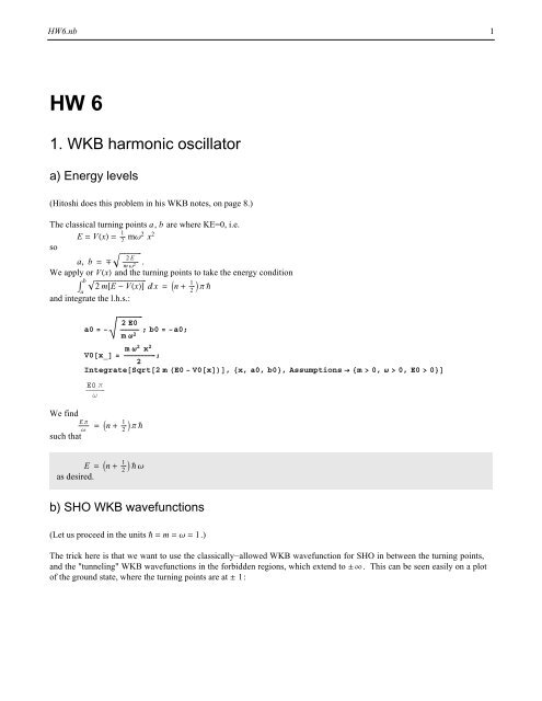
a) Energy levels
(Hitoshi does this problem in his WKB notes, on page 8.)
The classical turning points a, b are where KE=0, i.e.
E Vx 1
mΩ 2 2 x2 so
a, b 2E
m Ω2 .
We apply or Vx and the turning points to take the energy condition
b
2mE Vx x n
a
1
Π 2
and integrate the l.h.s.:
We find E Π
a0 2E0
; b0 a0;
m Ω2 V0x_ m Ω2 x2 ;
2
IntegrateSqrt2mE0 V0x, x, a0, b0, Assumptions m 0, Ω 0, E0 0
E0 Π
Ω
n Ω 1
Π 2
such that
E n 1
Ω 2
as desired.
b) SHO WKB wavefunctions
(Let us proceed in the units m Ω 1.)
The trick here is that we want to use the classically−allowed WKB wavefunction for SHO in between the turning points,
and the "tunneling" WKB wavefunctions in the forbidden regions, which extend to . This can be seen easily on a plot
of the ground state, where the turning points are at 1:

HW6.nb 2
PlotΠ14 Exp x2 x2
, , x, 2, 2, PlotStyle Dashing, Dashing.05, .05;
2 2
2
1.5
1
0.5
-2 -1 1 2
Our SHO energies (from part (a)), potential function, and classical turning points are:
Enn_ n 1
2 ;
Vx_ x2
;
2
an_
2 Enn ;
bn_ an;
We construct the wavefunction in allowed region using Eq. 30 in the notes. We split up the integral around x 0 and
consider the two turning points a and b separately, so Mathematica doesn’t give a trivial result:
Ψa1x_, n_
2AbsV ’an
13
Π
CosIntegrate
2Enn Vx
2Enn Vt ,
t, an, x, Assumptions n 0, an x, x 0 Π
;
4
12
12
Ψa2x_, n_
2AbsV ’bn
13
Π
CosIntegrate
2Enn Vx
2Enn Vt , t, x, bn, Assumptions n 0, x 0, x bn Π
;
4
Similarly, for the forbidden regions we use Eq. 31:
12
Ψf1x_, n_
2AbsV ’an
13
Π
2Vx Enn
1
2
ExpIntegrate
2Vt Enn , t, x, an, Assumptions n 0, x an;
12
Ψf2x_, n_
2AbsV ’bn
13
Π
2Vx Enn
1
2
ExpIntegrate
2Vt Enn , t, bn, x, Assumptions n 0, x bn;

HW6.nb 3
Ok, now what about the regions right around the classical turning points a and b? We know that the wavefunctions above
blow up near these points. So, let’s define a radius about the turning points inside which we treat specially:
Ε 0.5;
Next, we construct a piecewise function from the asymptotic wavefunctions above outside these regions (using ’UnitStep’):
Ψwkbasyx_, n_ 1 n Ψf1x, n1 UnitStepx an Ε
1 n Ψa1x, nUnitStepx an Ε1 UnitStepx
Ψa2x, nUnitStepx1 UnitStepx bn Ε Ψf2x, nUnitStepx bn Ε;
Now, in the special regions, we use the Airy functions themselves, and again construct a piecewise function:
Ψwkbtpax_, n_ 1 n AiryAi2AbsV ’an 13 x anUnitStepx an Ε
1 UnitStepx an Ε AiryAi2AbsV ’bn 13 x bn
UnitStepx bn Ε1 UnitStepx bn Ε;
Finally, we add these two chunks to get the whole function:
Ψwkbx_, n_ Ψwkbasyx, n Ψwkbtpax, n;
WAIT: If we’re using the asymptotic wavefunctions mated to the actual Airy functions in the transition regions, why not
just use the Airy functions everywhere, expanding about the turning points? A moment’s reflection gives the answer: this
would work great coming in from and passing through the turning points, but as you move into the classically−allowed
region, the Airy function would not reach its cosine−shaped asymptote fast enough! The reason we do it piecewise is that
we want accurate results where E V , and live with nastiness in the transition regions. (In the classically−forbidden
regions, the Airy function should decay fast enough to match the asymptotic solution.)
To see this, let’s construct this all−Airy function wavefunction by expanding around the two turning points:
Ψairx_, n_ 1 n AiryAi2AbsV ’an 13 x an1 UnitStepx
AiryAi2AbsV ’bn 13 x bnUnitStepx;
Finally, we wish to compare to the exact results:
1
Ψexax_, n_
2n Π
Factorialn
14 Exp x2
HermiteHn, x;
2
Let’s compare the exact and WKB solutions for n 1:

HW6.nb 4
PlotΨexax, 1, Ψwkbx, 1, x, 4, 4, PlotStyle GrayLevel0, Hue0;
0.6
0.4
0.2
-4 -2 2 4
-0.2
-0.4
-0.6
Our WKB solutions looks great at x and x 0 where E V and E V respectively, as expected. The Airy
function matches nicely with the decaying wavefunctions in the forbidden regions, but does indeed mismatch the wavefunction
in the allowed region.
Now, let’s compare the exact and all−Airy solutions:
PlotΨexax, 1, Ψairx, 1, x, 4, 4, PlotStyle GrayLevel0, Hue0;
0.6
0.4
0.2
-4 -2 2 4
-0.2
-0.4
-0.6
As expected, we get the opposite behavior. Coming in from , the wavefunction matches the exact solution nicely.
However, as we move toward x 0, the discrepancy builds up until you get a mismatch.
Now let’s look at n 10:

HW6.nb 5
PlotΨexax, 10, Ψwkbx, 10, x, 7, 7, PlotStyle GrayLevel0, Hue0;
0.4
0.2
-6 -4 -2 2 4 6
-0.2
-0.4
Fantastic! Because the energy is much higher, the approximation is far more accurate (i.e, the state is much more classical),
and on this plot the mismatch between the Airy function in the transition region and the wavefunction in the allowed region
is not even visible.
Now let’s look at the all−Airy solution for n 10:
PlotΨexax, 10, Ψairx, 10, x, 7, 7, PlotStyle GrayLevel0, Hue0;
0.4
0.2
-6 -4 -2 2 4 6
-0.2
-0.4
A bit better than n 1. The discrepancy builds up again coming toward x 0 from the turning points; however, because n
is even, there is no mismatch at x 0, just a sharp point.
Finally, let us look at n 20:

HW6.nb 6
PlotΨexax, 20, Ψwkbx, 20, x, 10, 10, PlotStyle GrayLevel0, Hue0;
0.4
0.2
-10 -5 5 10
-0.2
-0.4
We see that the WKB solution has a bit of overshoot due to the higher energy; otherwise the agreement is quite good.
Finally, let us compare the exact and all−Airy solutions for n 20:
PlotΨexax, 20, Ψairx, 20, x, 10, 10, PlotStyle GrayLevel0, Hue0;
0.4
0.2
-10 -5 5 10
-0.2
-0.4
The overshoot is still there, but the discrepancy is less approaching x 0 as one would expect with the higher energy.
N.B.: Of course, one could just use polynomial to handle the transition regions. But, if we’re going to use numerical
methods, we might as well use the variational method instead of WKB. :P

HW6.nb 7
2. Classical limit of hydrogen atom
a) Correspondence between orbital motion and emitted photon
One can derive the Bohr model by taking the energy of an electron circling a proton (CGS units)
E 1
m v 2 2 Z e2
r
and applying the quantization condition
Ln m v r n .
(This justification for this quantization is just units; we know that the ground state in fact has no angular momentum. One
can also derive the Bohr model by requiring whole wavelengths to fit on a circle of radius r.)
Substituting for v, we get
E 1 n
m 2 m r 2
Z e2
. r
We require one more condition to eliminate r. Let us use the force balance
m v2
Z e2
F
r r2 which gives
Z e2
r m v2 Z e2
m
and finally
rn n2 2
m r
n 2
Z e2 m .
Substituting this back in to the energy,
En 1
to obtain
En Z2 e4 m
Similarly,
vn
2 n2 2 m rn 2 Z e2
rn n2 2 n
m rn
2n 2 2 .
n
m Z e2 m
n2 2
2m Z e2 m
Z e2
n .
n 2 2 2
Z e2 Z e2 m
n2 2
Having derived these basic quantities, we can express the frequency of orbital motion in state n as
Νo vn
Z e2
2Π rn 2Π n
n3 3 .
On the other hand, we know that the frequency of a photon due to a change from state n to n k is
ΝΓ En Enk 1
2Π 2Π
Z2 e4 m
23 1
n2 1
nk 2 1
2Π
Z2 e4 m
2n2 3
1
1 k
n 2 1
Approximating k n,
.
ΝΓ 1
2Π
Z2 e4 m
2n2 3 1 2k
1
1
n 2Π Z2 e4 m
n3 3 k.
1
Z e2 m
n2 2 1
2Π Z2 e4 m
As indicated in the hint, we find that the frequency of the photon ΝΓ is an integer multiple of the frequency of orbital
motion Νo .

HW6.nb 8
b) Correspondence between classical radiation and mean lifetime
Under classical dynamics the electron is being continually accelerated, so it should emit radiation. To know the mean
lifetime Τ of a state n, we must know how fast it loses power. Since the model is semiclassical, we can use a classical
radiation formula. We found above that the velocity goes like 1
, so the motion at large n is non−relativistic and so we can
n
just use the Larmor power formula (again in CGS)
.
From above,
P 2e2 a2 3c3
an Fn
Substituting,
m
P 2Z6 e 14 m 2
.
3c 3 n 8 8
Z e2
m rn 2
The mean lifetime should be
Rearranging,
Z e2
m Z e2 m
n2 2 2
Z3 e6 m
n4 4 Τ En En1 P
Z2 e4 m
n3 2 1 3c3 n8 8
as expected.
1
Τ 2
3 e2 Z e2
c c 4
m c2
1
n5 2Z 6 e 14 m 2 3c3 n 5 6
.
Z 4 e 10 m .
c) Comparison of classical and quantum lifetimes
We implement the correct expression above (with in units of eV s):
lifetimecn_
2
ΑZ Α
3 4 mec2 1
hbar n5
Computing for n 2, 4, 6 we find respectively
2, 4, 6 lifetimec
1
2.98388 10 9 , 9.54841 10 8 , 7.25082 10 7
. Α 137 1 , Z 1, mec2 511000, hbar 6.582 10 16 ;
These are accurate to within an order of magnitude of the given quantum values, and seem to improve with increasing n as
we would expect.

HW6.nb 9
3. Spin precession in magnetic field
a) Time evolution of eigenstates
The Schrödinger equation is
e
e B
i t Ψ H Ψ g S B Ψ g
2m c 2m c Sz Ψ Ω Sz Ψ
where we defined Ω g
e B
2m c .
Then, for Ψ Sz ; we have
i t Sz ; Ω
2 Sz ;
and for Ψ Sz ; we have
i t Sz ; Ω
2 Sz ; .
So we have for the solutions
Sz ; , t e
Sz ; , t e
Ω
i
i Ω
2 t Sz ;
2 t Sz ; .
For a state aligned with the quantization axis, the "precession" is just a rotating phase.
b) Dynamics of S x ;
First, define the spin matrices:
Sx
2 0, 1, 1, 0;
Sy
2 0, I, I, 0;
Sz
2 1, 0, 0, 1;
Find the eigenstates of Sx :
eigenx EigensystemSx
,
2
, 1, 1, 1, 1
2
Our state Sx ; is then
and so
Sx ; 1
Sz ; Sz ;
2
Sx ; , t 1
Sz ; , t Sz ; , t .
2
In component form on the time−independent basis Sz ; , Sz ; ,

Our state Sx ; is then
Sx ; 1
Sz ; Sz ;
HW6.nb 2 10
and so
Sx ; , t 1
Sz ; , t Sz ; , t .
2
In component form on the time−independent basis Sz ; , Sz ; ,
Sx ; , t 1
2
e
Ω
ei
2 t
Ω
i
c) Showing precession
2 t
.
Let us implement the above state in component form, as well as its conjugate−transpose:
1
Ψsxpt_
ExpI
2
Ω
t, ExpI
2 Ω
t;
2
1
Ψsxpctt_
ExpI
2
Ω
t, ExpI
2 Ω
t;
2
We calculate Sx ; , t S
Sx ; , t and put it into vector x, y, z form:
ExpToTrigΨsxpctt.Sx .Ψsxpt1, 1,
Ψsxpctt.Sy .Ψsxpt1, 1, Ψsxpctt.Sz .Ψsxpt1, 1
1
Cost Ω,
2 1
Sint Ω, 0
2
This is the clockwise precession about the z−axis with angular frequency Ω g of a vector of length . As
2m c 2
expected, there is no z−component. (The classical analogue is a gyroscope precessing clockwise in the plane; of course,
here we can’t simultaneously have components of x/y and z.)
4. Hamilton−Jacobi for light [optional]
a) Apply WKB approximation to equation of motion
Following the same steps we did for the Schrödinger equation, we first write the Maxwell’s equation with A 0 e i S :
n2
c2 2
t2 2
ei S
n2
c2
i S
i S
2
i 2 S
i S
2
ei S 0 .
In the limit S , we can drop terms of OS and keep those of OS 2 :
n2 c2 2
S
S 2 0.
This is the "Hamilton−Jacobi" equation.
e B

HW6.nb 11
(Of course, in the Maxwell equation, there is no notion of . What we are doing is a valid approximation when the variation
of the phase is very fast compared to the variation of the index of refraction. It is called "eikonal approximation" in optics.)
b) Equivalence to particle in given potential
The Hamiltonian of free particle in potential Vx 1
2m nx 2
H p2
2m
n2
2m .
Applying this to the Hamilton−Jacobi equation, we obtain
1
2m
2
S
n2
2m
S
0. t
Since the action has no explicit time dependence, we can make the Legendre transformation St, x S E, x E t to get
and finally
2
1
2m S
n2
E 0
2m
n2
S 2
0.
If n in part (a) has no time dependence, we can do the same Legendre transformation and obtain the equivalent "H−J"
equation
E
n c 2
S 2
0.
c) Separate variables, integrate "action" variable
Assuming nx nx, the "Hamilton−Jacobi" equation does not have an explicit dependence on y or t. Writing
Sx, y, t S
x, py , E py y E t,
the equation becomes
n 2
Therefore,
c2 E2 d
d S
d x
and hence
d x S
n2
c2 E2 py 2
S
x
2 py 2 0.
E2 py 2 d x’.
nx’ 2
c2 Here, the possible x−dependence of the index of refraction is emphasized.
is

HW6.nb 12
S
x
E2 py 2 d x’.
nx’ 2
c2 Here, the possible x−dependence of the index of refraction is emphasized.
d) Integral expressions for "angle" variables
S
S
Using t , y , we find
E
t
y
x
x
py
nx’ 2
c 2 E
d x’,
nx’2
c2 E2 py 2
py
nx’2
c2 E2 py 2
e) Work to Snell’s law
d x’.
Assuming that nx n1 for x 0 and nx n2 for x 0, and choosing the lower end of the integration at x 0,
and
y x
y x
py
n 2
1
c2 E2 py 2
py
n 2
2
c2 E2 py 2
x for x 0
x for x 0.
1
cot2 Α1
Using the trigonometric relation sin Α , we find
and hence
1
c py
sin Α n1 E ,
n 2
1 E2 py 2
c2 1
py 2
1
c py
sin Α n2 E ,
sin Α
sin Α
n 2
2 E2 py 2
c2 1
,
n2 n1
py 2
which is nothing but the Snell’s law of refraction.