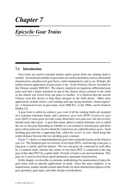
Chapter 07: Epicyclic Gear Trains

Chapter 7
Epicyclic Gear Trains
7.1 Introduction
Gear trains are used to transmit motion and/or power from one rotating shaft to
another. An enormous number of gear trains are used in machinery such as automobile
transmissions, machine tool gear boxes, robot manipulators, and so on. Perhaps, the
earliest known application of gear trains is the South Pointing Chariot invented by
the Chinese around 2600 B.C. The chariot employed an ingenious differential gear
train such that a figure mounted on top of the chariot always pointed to the south
as the chariot was towed from one place to another. It is believed that the ancient
Chinese used this device to help them navigate in the Gobi desert. Other early
applications include clocks, cord winding and rope laying machines, steam engines,
etc. A historical review of gear trains, from 3000 B.C. to the 1960s, can be found in
Dudley [3].
A gear train is called an ordinary gear train if all the rotating shafts are mounted
on a common stationary frame, and a planetary gear train (PGT) or epicyclic gear
train (EGT) if some gears not only rotate about their own joint axes, but also revolve
around some other gears. A gear that rotates about a central stationary axis is called
the sun or ring gear depending on whether it is an external or internal gear, and those
gears whose joint axes revolve about the central axis are called the planet gears. Each
meshing gear pair has a supporting link, called the carrier or arm, which keeps the
center distance between the two meshing gears constant.
Figure 7.1 shows a compound planetary gear train commonly known as the Simpson
gear set. The Simpson gear set consists of two basic PGTs, each having a sun gear, a
ring gear, a carrier, and four planets. The two sun gears are connected to each other
by a common shaft, whereas the carrier of one basic PGT is connected to the ring
gear of the other PGT by a spline shaft. Overall, it forms a one-dof mechanism. This
gear set is used in most three-speed automotive automatic transmissions.
In this chapter, we describe a systematic methodology for enumeration of epicyclic
gear trains with no specific applications in mind. Since the main emphasis is on
enumeration, readers should consult other books for more detailed descriptions of the
gear geometry, gear types, and other design considerations.

FIGURE 7.1
Compound planetary gear train.
7.2 Structural Characteristics
Epicyclic gear trains belong to a special class of geared kinematic chains. In
addition to satisfying the general structural characteristics outlined in Chapters 4 and
6, the following constraints are imposed [2]:
1. All links of an epicyclic gear train are capable of unlimited rotation.
2. For each gear pair, there exists a carrier, which keeps the center distance between
the two meshing gears constant.
Based on the above two constraints, the geared five-bar mechanism discussed in
Chapter 6 is not an epicyclic gear train. In what follows, we study the effects of these
two constraints on the structural characteristics of epicyclic gear trains.
For all links to possess unlimited rotation, the prismatic joint is excluded from
design consideration. Hence only revolute joints and gear pairs are allowed for

structure synthesis of EGTs. For convenience, we use a thin edge to represent a
revolute joint (or turning pair) and a thick edge to stand for a gear pair. For this
reason, thin edges are sometimes called turning-pair edges and thick edges are called
geared edges.
Let jg denote the number of gear pairs and jt represent the number of revolute
joints. It is clear that the total number of joints is given by
j = jt + jg . (7.1)
Substituting Equations (6.7) and (7.1) into Equation (4.3), we obtain
F = 3(n − 1) − 2jt − jg . (7.2)
The first constraint implies that there should not be any circuit formed exclusively
by turning pairs. Otherwise, either the circuit will be locked or rotation of the links
will be limited. The second constraint implies that all vertices should have at least
one incident edge that represents a turning pair. Hence, we have
THEOREM 7.1
The subgraph obtained by removing all geared edges from the graph of an EGT is a
tree.
Since a tree of v vertices contains v − 1 edges, we further conclude that
jt = n − 1 . (7.3)
Substituting Equations (7.1) and (7.3) into Equation (4.5), we obtain
jg = L. (7.4)
Substituting Equations (7.3) and (7.4) into Equation (7.2) yields
L = n − 1 − F = jt − F. (7.5)
Eliminating jt and jg from Equations (7.1), (7.4), and (7.5) yields
j = F + 2L, (7.6)
Summarizing Equations (7.3), (7.4), and (7.5) in words, we have
THEOREM 7.2
In epicyclic gear trains, the number of gear pairs is equal to the number of independent
loops; the number of turning pairs is equal to the number of links diminished by one;
and the number of degrees of freedom is equal to the difference between the number
of turning pairs and the number of gear pairs.

In Chapter 4, we have shown that the degree of a vertex is bounded by Equation
(4.10). In terms of kinematic chains,
In words, we have:
L + 1 ≥ di ≥ 2 . (7.7)
THEOREM 7.3
The degree of any vertex in the graph of an EGT lies between 2 and L + 1.
In general, the graph of an EGT should not contain any circuit that is made up
of only geared edges. Otherwise, the gear train may rely on special link length
proportions to achieve mobility. In the case where geared edges form a loop, the
number of edges must be even. For example, Figure 7.2 shows a two-dof differential
gear train in which gears 3, 4, 5, and 6 form a loop. The four gears are sized such that
the pitch diameter of gear 3 is equal to that of gear 5, and the pitch diameter of gear 4
is equal to that of gear 6. Otherwise, the mechanism will not function properly. In
fact, we may consider either gear 4 or 6 as a redundant link. That is, removing either
gear 4 or 6 from the mechanism does not affect the mobility of the mechanism. This
is a typical fractionated mechanism in that links 2, 3, 4, 5, and 6 form a one-dof gear
train and the second degree of freedom comes from the fact that the gear train itself
can rotate as a rigid body about the “a–a” axis.
FIGURE 7.2
A differential gear train.

Recall that the subgraph obtained by removing all geared edges from the graph of
an EGT is a tree. Any geared edge added onto the tree forms a unique circuit called
the fundamental circuit. In other words, each fundamental circuit is made up of one
geared edge and several turning-pair edges. These turning pairs are responsible for
maintaining a constant center distance between the two gears paired by the geared
edge. Therefore, the axes of all turning pairs in a fundamental circuit can be associated
with two distinct lines in space, one passing through the axis of one gear and the other
passing through the axis of the second gear.
Let each turning-pair edge be labeled by a letter called the level. In this manner,
each label or level denotes an axis of a turning pair in space. We define the turningpair
edges that are adjacent to the geared edge of a fundamental circuit as the terminal
edges. Then, the requirement for constant center distance between two meshing gears
can be stated as:
THEOREM 7.4
In an EGT, there are two and only two edge levels between the terminal edges of a
fundamental circuit. In other words, there exists one and only one vertex, called the
transfer vertex, in each fundamental circuit such that all the turning-pair edges lying
on one side of the transfer vertex share one edge level and all the other turning-pair
edges lying on the opposite side of the transfer vertex share a different level.
The transfer vertex of a fundamental circuit corresponds to the carrier or arm of
a gear pair. We note that a vertex in the graph of an EGT may serve as the transfer
vertex for more than one fundamental circuit. From a mechanical point of view, any
vertex having only two incident turning-pair edges must serve as the transfer vertex
of a fundamental circuit.
A graph having several turning-pair edges of the same level implies that there are
several coaxial links in the corresponding kinematic chain. Hence,
COROLLARY 7.1
All edges of the same level in the graph of an EGT together with their end vertices
form a tree.
For example, Figure 7.3a depicts the schematic diagram of the Simpson gear set
shown in Figure 7.1. The corresponding graph with its turning pair edges labeled
according to their axis locations is shown in Figure 7.3b. Readers can easily verify
that Equations (7.3) through (7.5) are satisfied. Removing all the geared edges from
the graph leads to a spanning tree as shown Figure 7.3c. Putting the geared edges back
on the tree one at a time results in four fundamental circuits as shown in Figures 7.3d
through g. From the above corollary, we see that the transfer vertices of these four
fundamental circuits are 1, 1, 2, and 2, respectively.

FIGURE 7.3
Graph, spanning tree, and fundamental circuits of an EGT.

We summarize the structural characteristics for the graphs of EGTs as follows:
C1. The graph of an F -dof, n-link EGT contains (n − 1) turning-pair edges and
n − 1 − F geared edges.
C2. The subgraph obtained by removing all geared edges from the graph of an EGT
is a tree.
C3. Any geared edge added onto the tree forms one unique circuit, called the fundamental
circuit having one geared edge and several turning-pair edges. Consequently,
the number of fundamental circuits is equal to the number of geared
edges.
C4. Each turning-pair edge can be characterized by a level that identifies the axis
location in space.
C5. There exists a vertex, called the transfer vertex, in each fundamental circuit
such that all turning-pair edges lying on one side of the transfer vertex have the
same edge level and all turning-pair edges on the opposite side of the transfer
vertex share a different edge level.
C6. Any vertex that has only thin edges incident to it must serve as a transfer vertex
of at least one fundamental circuit. In other words, no vertex can have all its
incident edges on the same level.
C7. Turning-pair edges of the same level and their end vertices form a tree.
C8. The graph of an EGT should not contain any circuit that is made up of only
geared edges.
7.3 Buchsbaum–Freudenstein Method
The structural characteristics discussed in the previous section are applicable for
both spur and bevel gear trains. Any graph that satisfies the criteria represents a
feasible solution. Several heuristic methods of enumeration have been developed by
researchers. Perhaps, the first methodology was due to Buchsbaum and Freudenstein
[2]. The method involves the following steps:
S1. Determination of nonisomorphic unlabeled graphs (no distinction between
turning and gear pairs).
Given the number of degrees of freedom and the number of links, we search for
those unlabeled graphs that satisfy the first structural characteristic, C1, from the
atlas of graphs listed in Appendix C. These graphs are classified in accordance
with the number of degrees of freedom, number of independent loops, and

FIGURE 7.4
Unlabeled graphs of one-dof EGTs.
vertex-degree listing. Figures 7.4 and 7.5 provide all the feasible unlabeled
graphs for one- and two-dof gear trains having one to three independent loops.
S2. Determination of nonisomorphic bicolored graphs.
For each graph obtained in S1, we need to find structurally distinct ways of
coloring the edges, one color for the gear pairs and the other for the turning
pairs. Specifically, jg edges of the unlabeled graph are to be assigned as the
gear pairs and the remaining edges as the turning pairs. The solution to this
problem can be regarded as the number of combinations of j elements taken
jg at a time without repetition. From combinatorial analysis, it can be shown

FIGURE 7.5
Unlabeled graphs of two-dof EGTs.
that there are
C j
jg =
j!
jg!
j − jg !
(7.8)
possible ways of coloring the edges. A computer program employing a nesteddo
loops algorithm can be written to find all possible combinations. For example,
we may treat the edges as x1,x2,...,xj variables and solve Equation (7.9)
for all possible solutions of x1,x2,...,xj in ones and zeros, where the “1” represents
a gear pair and the “0” a turning pair.
x1 + x2 +···+xj = jg . (7.9)
We note that some of the graphs obtained by this process may be isomorphic,
others may violate the second structural characteristic, C2, and still others
may result in partially locked kinematic chains. Hence, the total number of

structurally distinct bicolored graphs would be fewer than the number predicted
by Equation (7.8).
For example, the 2210 graph shown in Figure 7.4 has five vertices and seven
edges. From the structural characteristic C1, we know that three of the seven
edges are to be assigned as gear pairs and the remaining edges as turning pairs.
Equation (7.8) predicts 7!/(3!4!) = 35 possible combinations. After screening
out those graphs that do not obey the second structural characteristic, and after
eliminating isomorphic graphs, we obtain 12 structurally distinct bicolored
graphs as shown in Figure 7.6.
FIGURE 7.6
Bicolored graphs derived from the 2210 graph.
S3. Determination of edge levels.
In this step, the fundamental circuits associated with each bicolored graph
derived in the preceding step are identified by applying the third structural
characteristic, C3. Then, the turning-pair edges within each fundamental circuit
are labeled according to the remaining structural characteristics, C4 through
C8. In labeling the turning-pair edges, it is more convenient to start with those
fundamental circuits that have fewer numbers of turning-pair edges. In this
way, the edge levels can be easily determined by observation. In addition,
the number of possible assignments of edge levels for the subsequent circuits
is reduced by the fact that some of the edges have already been determined
from the preceding circuits. The procedure is continued until all the possible
assignments of edge levels are exhausted or the graph is judged to be infeasible.

Consider the graph shown in Figure 7.7a. We start the labeling with the fundamental
circuit formed by vertices 1–4–5–1 as shown in Figure 7.7b. Since there
are only two turning-pair edges, we can arbitrarily assign a level “a” to the 4–5
edge and a different level “b” to the 1–4 edge. In this regard, vertex 4 serves as
the transfer vertex for the circuit. Next, we consider the fundamental circuit defined
by the vertices 1–3–4–1. Again, there are only two turning-pair edges associated
with the circuit. However, the 1–4 edge level has already been assigned
from the previous circuit. Thus, we only need to determine the level of the 3–4
edge. We can assign a new level “c,” or use an existing level “a” for the 3-4 edge
asshowninFigures7.7canddwithoutviolatingthestructuralcharacteristicsC4
through C8. Finally, we consider the fundamental circuit formed by vertices
1–4–3–2–1. Although there are three turning-pair edges associated with the
circuit, two of them have already been determined from the other two circuits.
Thus, the third edge can be easily determined by observing the fifth structural
characteristic, C5. The labeled graphs are shown in Figures 7.7g and h.
As another example, consider the graph shown in Figure 7.8. There are three
fundamental circuits. We start the labeling with the circuit formed by vertices 1–
4–5–1. Since there are only two turning-pair edges, we can arbitrarily assign
a level “a” to the 4–5 edge and a different level “b” to the 1–5 edge. Next, we
consider the fundamental circuit defined by the vertices 1–2–3–1. There are
only two turning-pair edges associated with this circuit. None of them have
been defined from the preceding circuit. Hence, we can arbitrarily assign a new
level “c” to the 1–2 edge and another level “d” to the 2–3 edge. This completes
the assignment of the second circuit. Finally, we consider the fundamental
circuit defined by the vertices 3–2–1–5–4–3. We notice that all the turningpair
edges have already been determined from the other two circuits. A careful
examination of the labeling reveals that this circuit contains too many levels,
violating the fifth structural characteristic, C5. Hence, we conclude that this
graph is not feasible. In fact, this graph should be excluded from the outset
since it contains a circuit 1–3–4–1 formed exclusively by geared edges.
S4. Determination of the type of gear meshes.
The two gears paired by each geared edge can assume an external-to-external,
external-to-internal, or internal-to-external gear mesh. Therefore, there are 3 jg
possible gear mesh arrangements for each labeled graph obtained in S3. Again,
some of the arrangements may result in isomorphic mechanisms and should be
screened out.
S5. Sketching of the corresponding functional schematics.
In this step, we sketch the functional schematic of each labeled graph. Here we
treat an edge of a graph as defining the connection between two links and the
thin edge level as defining the axis location of a turning pair. The functional
schematic of a labeled graph can be sketched by adhering to the following
guidelines.

FIGURE 7.7
Two different labelings of turning-pair edges.

FIGURE 7.8
A labeled graph that violates the structural characteristics.
1. Sketch a line for each thin edge level. We note that these lines should be
drawn parallel to one another for planar epicyclic gear trains, and intersecting
at a common point for bevel gear trains. The arrangement of these
lines is rather arbitrary and it may occasionally require a rearrangement
in order to produce a nice-looking functional mechanism.
2. For each fundamental circuit, draw a pair of gears with their axes of
rotation passing through the corresponding center lines defined by the
levels of the terminal edges. Connect all gears of the same link number.
3. Draw the remaining links, if any, with their joint axes located on the
appropriate center lines in accordance with the edge levels.
4. Complete the remaining turning-pair connections according to the levels
of the graph.
For example, Figure 7.9a shows a labeled graph with three fundamental circuits.
In sketching the functional schematic of the gear train, we first draw three
parallel lines “a,” “b,” and “c” as shown in Figure 7.9b. Then, for the 2–1–
3–2 fundamental circuit, we draw a pair of gears (2 and 3) with their axes
of rotation passing through the two center lines “a” and “b;” for the 3–1–4–
3 fundamental circuit, we draw a second pair of gears (3 and 4) with their
rotation axes passing through the center lines “b” and “a;” and for the 4–1–5–4
fundamental circuit, we sketch a third pair of gears (4 and 5) with their axes
passing through the center lines “a” and “c,” respectively. We note that link 3
appears in the first and second fundamental circuits. Hence, these two gears
are connected as one link. Similarly, link 4 appears in the second and third
circuits and, therefore, these two gears are also connected as one link. Finally,
we draw link 1, which is the transfer vertex for all fundamental circuits, with its
axes of rotation passing through the center lines “a,” “b,” and “c,” and complete
all the turning-pair connections in accordance with the edge levels shown in
Figure 7.9a. This procedure can be automated by a computer program with a
graphical input-output feature.

FIGURE 7.9
Sketching of an EGT.
7.4 Genetic Graph Approach
Buchsbaum and Freudenstein’s method is a powerful tool for enumeration of EGTs
in a systematic and unbiased manner. However, the process becomes more involved
as the number of links increases. In this section, we introduce an alternative method
called the genetic graph approach to improve the efficiency [14].
This approach uses the graph of a basic gear train, called the genetic graph, as a
building block. In view of the first structural characteristic, each time we increase
the number of vertices by one, we also increase the number of loops, the number
of turning-pair edges, and the number of geared edges by one. The new vertex can
be connected to any vertex of the genetic graph by a turning-pair edge, and to any
other vertex by a geared edge, as shown in Figure 7.10a. In this way, n(n− 1) new
unlabeled graphs are generated from a genetic graph of n vertices. However, some of
the graphs may be rejected due to violation of the structural characteristics, whereas
others may be isomorphic to one another. Hence, the total number of nonisomorphic
unlabeled graphs is usually fewer than n(n − 1).
The procedure can be automated by a computer program using the adjacency matrix
notation and a nested-do loops algorithm. Specifically, we start with a given adjacency
matrix of order n. Each time we increase the number of vertices by one, we add a
row and a corresponding column to the matrix. We first initialize all elements of the
new row and the corresponding column to zero. Then we assign a “1” to one element
(excluding the diagonal element) in the newly added row (and the corresponding
column) for a turning pair, and a “g” to another element for a gear pair. This results

FIGURE 7.10
Enumeration of EGTs.
in a matrix of order n + 1, representing a new gear train having n + 1 links. The
process is repeated until all the possible arrangements are exhausted. Finally, graph
isomorphisms are checked. Figure 7.10b illustrates the concept of extending a 3 × 3
matrix to a 4 × 4 matrix. The upper-left 3 × 3 submatrix represents the genetic graph
shown in Figure 7.10a, and the elements with a pound sign in the fourth row and
fourth column are to be filled with a “1” and a “g.” Using this methodology, the first
three structural characteristics are automatically satisfied. The process is similar to
the conventional method of designing gear trains. A designer starts with a simple
gear train and increases the complexity of the design by adding one gear at a time.
When a new gear is added, a journal bearing is also incorporated to support the gear.
The approach has been successfully employed for the enumeration of one-dof EGTs
with up to five independent loops [9, 14], and the enumeration of two-dof EGTs [16].
7.5 Parent Bar Linkage Method
In this section we introduce another approach called the parent bar linkage technique
[13]. The parent of a mechanism is defined as that bar linkage that is generated
by replacing each q-dof joint in the mechanism with a binary-link chain of length
q− 1. For example, Figures 7.11a and c show the functional schematic and graph
representations of an EGT with two gear pairs. The parent bar linkage is obtained

y replacing each gear pair by two turning pairs and one intermediate binary link as
shown in Figures 7.11b and d. We note that the process of joint substitution has no
effect on the mobility of a mechanism. The above process can also be reversed; that
is, a mechanism with multi-dof joints can be generated by replacing a binary-link
chain of length q − 1 in a parent bar linkage by a q-dof joint.
FIGURE 7.11
An epicyclic gear train and its parent bar linkage.
By definition, parent bar linkages have the same number of loops and number of
degrees of freedom as the mechanisms generated. Hence, the atlas of bar linkages
listed in Appendix D can be used as a basis for generating epicyclic gear trains of the
same nature, i.e., same number of degrees of freedom, F , and number of independent
loops, L. In general, an n-link bar linkage can be used to construct a gear train,
provided that there are at least L number of binary links in the parent bar linkage.
The method can summarized as follows.
1. Identify planar bar linkages with the desired number of degrees of freedom,
F , and number of independent loops, L, from the atlas of graphs listed in
Appendix D. Those parent bar linkages should contain at least one binary
vertex in each loop.
2. Replace one binary vertex in each loop along with its incident edges by a geared
edge.

3. Eliminate those graphs that do not obey the first and second structural
characteristics.
4. Assign a level to each thin edge in accordance with the remaining structural
characteristics. This results in a family of EGTs that have the same number
of degrees of freedom and number of independent loops as that of the parent
bar linkages.
5. Sketch the corresponding functional schematics.
This method can be very efficient, provided that an atlas of parent bar linkages
already exists [8, 13].
7.6 Mechanism Pseudoisomorphisms
Since the edges of a graph represent the joints of a kinematic chain, multiple joints
cannot be properly represented. For this reason, a ternary joint is represented by
two coaxial binary joints, a quaternary joint by three coaxial binary joints, and so on.
This notation, however, creates a problem in uniquely representing a mechanism with
multiple joints.
When there are several links in a mechanism sharing a common joint axis, it is
possible to reconfigure the pair connections among these coaxial links without affecting
the functionality of the mechanism. For the mechanism shown in Figure 7.12a,
links 1, 2, 3, and 4 share a common joint axis, “a.” Therefore, the revolute joints
connecting these four coaxial links can be reconfigured in several different ways.
Figure 7.12c shows a rearrangement of the revolute joints. The corresponding graphs
are shown in Figures 7.12b and d, respectively. Although these two mechanisms are
structurally nonisomorphic, they are kinematically equivalent. From the functional
point of view, they are considered to be isomorphic. Such kinematically equivalent
mechanisms and their corresponding graphs are called pseudoisomorphic mechanisms
and pseudoisomorphic graphs, respectively [4, 15].
Specifically, the graph shown in Figure 7.12d is obtained from the graph shown
in Figure 7.12b by replacing the 1–2 turning-pair edge with a 1–3 turning-pair edge
of the same level. The process of replacing a turning-pair edge with another of the
same level is called a vertex selection [4]. The number of possible vertex selections
increases with the number of coaxial links in a mechanism. This creates a need for
identification of pseudoisomorphisms. Alternatively, we can identify a unique graph
among all the possible pseudoisomorphic graphs as the canonical graph to represent
all the possible pseudoisomorphic graphs. The canonical graph representation is
defined for epicyclic gear trains with the fixed link clearly identified as the root. In

FIGURE 7.12
Pseudoisomorphic mechanisms and their graph representations.
canonical graph representation, all thin-edged paths that emanate from the root and
terminate at any other vertex have distinct edge levels. See Chapter 8 for more details.
7.7 Atlas of Epicyclic Gear Trains
Using the methods described in the preceding sections, epicyclic gear trains with
one, two, and three degrees of freedom and with up to four independent loops (four
gear pairs) have been enumerated by various researchers [2, 4, 13, 14, 16, 8]. Table 7.1
summarizes the number of labeled nonisomorphic graphs in terms of the number of
degrees of freedom and the number of independent loops. Appendix F provides an
atlas of labeled graphs and typical functional schematics of nonfractionated epicyclic

gear trains classified according to the number of degrees of freedom, number of
independent loops, and vertex degree listing.
Table 7.1
Trains.
Classification of Epicyclic Gear
Degrees of No. of No. of No. of No. of
Freedom Loops Links Joints Solutions
F L n j
1 1 3 3 1
2 4 5 3
3 5 7 13
4 6 9 80
2 1 4 4 0
2 5 6 0
3 6 8 3
4 7 10 50
3 1 5 5 0
2 6 7 0
3 7 9 0
4 8 11 8
7.7.1 One-dof Epicyclic Gear Trains
For one-dof epicyclic gear trains, there are 1 single-loop, 2 two-loop, 6 three-loop,
and 26 four-loop, unlabeled nonisomorphic graphs as shown in Figures 7.13 and 7.14.
These graphs can be labeled into 1 three-link, 3 four-link, 13 five-link, and 80 six-link,
labeled nonisomorphic graphs as shown in Tables F.1 through F.8, Appendix F.
One-dof EGTs are widely used as simple speed reducers, automotive transmission
mechanisms, and other power transmission mechanisms. Note that there exists a
graph that contains a circuit made up of only geared edges as shown in Figure 7.15.
Although this gear train violates the structural characteristic, C8, it does not require
special link length proportions to achieve mobility.
7.7.2 Two-dof Epicyclic Gear Trains
For two-dof epicyclic gear trains, there are no nonfractionated EGTs with one
or two independent loops. There are 3 labeled nonisomorphic graphs with three
independent loops as shown in Table F.9, Appendix F, and 50 labeled nonisomorphic
graphs with four independent loops. A skillful engineer can sketch a mechanism
from graph number 1 listed in Table F.9 into a two-dof robotic wrist as shown in
Figure 7.16. Graphs of two-dof EGTs with four independent loops can be found in
Tsai and Lin [16].

FIGURE 7.13
Unlabeled graphs of 3- to 5-link EGTs.
A two-dof coupling that maintains a constant velocity ratio between the input and
output shafts is shown in Figure 7.17. The coupling consists of two hinged frames,
links 1 and 2, that house three differential gear trains. The first differential, consisting
of bevel gears 3, 4, 5, and 6, determines the speed ratio between the input and output
shafts; the second differential, consisting of spur gears 2, 7, and 8, detects relative
rotation of the two frames; and the third differential, consisting of bevel gears 8, 9,
and 4, picks up the motion of the spur-gear differential to compensate for the velocity
fluctuation due to relative rotation of the two frames. The spur gears remain stationary
except when the two frames are changing their relative angular orientation. As one
frame rotates with respect to the other, the spur-gear train provides an input to the
third differential, which in turn either retards or advances the rotation of the first
differential keeping the velocity ratio constant at all times.
7.7.3 Three-dof Epicyclic Gear Trains
For three-dof epicyclic gear trains, there are no nonfractionated EGTs with one,
two, or three independent loops. Table F.10 in Appendix F gives 8 labeled graphs of
three-dof EGTs having four independent loops.

FIGURE 7.14
Unlabeled graphs of 6-link EGTs.
7.8 Kinematics of Epicyclic Gear Trains
Numerous methods for kinematic analysis of EGTs have been proposed by several
researchers [1, 6, 7, 10, 11, 12, 17]. The most straightforward approach makes use
of the theory of fundamental circuits introduced by Freudenstein and Yang [5]. The

FIGURE 7.15
An EGT having a circuit consisting of only geared edges.
FIGURE 7.16
A two-dof wrist mechanism.

FIGURE 7.17
Constant velocity-ratio drive.
method was subsequently modified by Tsai [15] for the kinematic analysis of bevelgear
robotic mechanisms. This method can be easily implemented on a computer for
automated analysis of EGTs.
7.8.1 Fundamental Circuit Equations
In the previous sections, we have shown that when all geared edges are taken off
the graph of an EGT, the remaining subgraph is a tree. When a geared edge is put
back onto the tree, it forms precisely one circuit called the fundamental circuit and
the number of fundamental circuits is equal to the number of gear pairs in the gear
train. In what follows, we show that a basic kinematic equation can be derived for
each fundamental circuit.
Let i and j be a gear pair and k be the carrier. Then links i, j, and k constitute a
simple gear train as illustrated in Figure 7.18. Since the tangential velocities at the
meshing point of the two gears with respect to the carrier are equal to one another, a
fundamental circuit equation can be written as
ωi − ωk =±Nj,i ωj − ωk , (7.10)
where ωi denotes the angular speed of link i, and Nji = Dj /Di = Tj /Ti represents

FIGURE 7.18
A gear pair and its fundamental circuit.
the gear ratio, whereDi and Ti are the pitch diameter and the number of teeth on gear
i. The sign in Equation (7.10) is positive if a positive rotation of gear i relative to the
carrier k produces a positive rotation of gearj, otherwise it is negative. By definition,
we have
Nik = 1
Nki
. (7.11)
Equation (7.10) is valid whether the gear train is a planar or bevel gear type and
whether the carrier is stationary or not. To facilitate the analysis, a positive direction
of rotation, zi-axis, is assigned to each joint axis of an epicyclic gear train. For planar
gear trains, it is most convenient to definethe positive direction of rotation of all gears
to be pointing out of the paper. In this way, we have a positive sign for an internal
gear pair and a negative sign for an external gear pair. For bevel gear trains, we
simplyassign a positive direction of rotation to each joint axis, and obtain the sign of
Equation (7.10) by following the above definition.Writing Equation (7.10) once for
each fundamental circuit of an epicyclic gear train results injg fundamental circuit
equations that can be solved for the speed ratios of any two gears.
7.8.2 Examples
Example 7.1 Minuteman Cover Drive
Refer to Figure 7.19 for the functional schematic and graph representation of the
Minuteman cover drive. In this mechanism, the first ring gear, link 1, is held stationary;
the sun gear, link 2, serves as the input link; and the other ring gear, link 5, is the
output link. The compound planet, link 4, meshes with the sun gear 2 and the two ring
gears and is supported by the carrier, link 3, by a revolute joint. Link 2 is connected

to links 1, 3, and 5 by revolute joints. Overall, it forms a one-dof compound planetary
gear train. We wish to find the speed reduction ratio for this mechanism.
FIGURE 7.19
Minuteman cover drive and its graph representation.
Since there are three gear pairs in the mechanism, the number of fundamental
circuits is equal to three. From the graph representation, we can easily identify the
three fundamental circuits as (2, 4)(3), (1, 4)(3), and (4, 5)(3). In this notation, the
first two numbers in the parentheses denote the gear pair and the third number denotes
the carrier. The fundamental circuit equations can be written as
ω2 − ω3 = −N42 (ω4 − ω3) , (7.12)
ω1 − ω3 = N41 (ω4 − ω3) , (7.13)
ω4 − ω3 = N54 (ω5 − ω3) . (7.14)
Since link 1 is fixed, ω1 = 0, identically. We treat ω2 as the input and ω5 as the
output of the gear train. Hence, we have three linear equations in three unknowns,
ω3, ω4, and ω5. Substituting Equation (7.14) into Equations (7.12) and (7.13) yields
ω2 − ω3 = −N42N54 (ω5 − ω3) , (7.15)
ω3 = −N41N54 (ω5 − ω3) , (7.16)
Solving Equation (7.16) for ω3 and substituting the resulting expression into Equation
(7.15) yields
ω5 = (N41N54 − 1)
N54 (N41 + N42) ω2 . (7.17)
Equation (7.17) gives the overall speed ratio of the gear train. For example, let

N41 = 32
74 , N42 = 33 9 , and N54 = 75
33 , then
ω2
ω5
=
75 32
33 74 + 33
9
32
74 · 75
=−542 .
33 − 1
We observe that a very large gear ratio can be obtained from a relatively simple and
compact gear train.
Example 7.2 Simpson Gear Train
Figure 7.20 shows a schematic diagram of the Simpson gear set, where link 1 is
grounded, link 4 serves as the input, and link 2 is the output. We wish to find the
speed ratio of the gear train.
FIGURE 7.20
Simpson gear train.
The graph representation of the gear train is shown in Figure 7.3. There are four
fundamental circuits: (5, 2)(1), (5, 3)(1), (6, 4)(2), and (6, 3)(2), and the fundamental
circuit equations are
ω5 − ω1 = +N25 (ω2 − ω1) , (7.18)
ω5 − ω1 = −N35 (ω3 − ω1) , (7.19)
ω6 − ω2 = +N46 (ω4 − ω2) , (7.20)
ω6 − ω2 = −N36 (ω3 − ω2) . (7.21)

Since link 1 is fixed, ω1 = 0, identically. We treat ω4 as the input and ω2 as the
output of the gear train. Hence, we have four linear equations in four unknowns, ω2,
ω3, ω5, and ω6. We need to eliminate ω3, ω5, and ω6 from these four equations.
Equating Equations (7.20) and (7.21) yields
N36 (ω3 − ω2) + N46 (ω4 − ω2) = 0 . (7.22)
Similarly, equating Equations (7.18) and (7.19) yields
N35ω3 + N25ω2 = 0 . (7.23)
Eliminating ω3 from Equations (7.22) and (7.23) yields the speed ratio as
ω4
= 1 +
ω2
N36
1 +
N46
N25
N35
. (7.24)
Let the gear sizes of the input planetary gear set be T4 = 70, T6 = 14, and T3 = 42;
and that of the output planetary gear set be T ′ 3 = 30, T5 = 16, and T2 = 62. Then we
have N46 = 5, N36 = 3, N25 = 3.875, and N35 = 1.875. Substituting these values
into Equation (7.24), we obtain
ω4
ω2
= 2.84 .
This is a typical reduction for the first gear of an automotive automatic transmission
mechanism.
Example 7.3 Constant Velocity-Ratio Drive
We wish to derive the speed ratio between the input and output shafts of the two-dof
differential gear train shown in Figure 7.17.
There are six fundamental circuits: (7, 2)(1); (8, 7)(1); (8, 9)(5); (9, 4)(5); (4, 3)(1);
and (5, 6)(2). The fundamental circuit equations are
ω7 − ω1 = −N27 (ω2 − ω1) , (7.25)
ω8 − ω1 = −N78 (ω7 − ω1) , (7.26)
ω8 − ω5 = −N98 (ω9 − ω5) , (7.27)
ω9 − ω5 = +N49 (ω4 − ω5) , (7.28)
ω4 − ω1 = +N34 (ω3 − ω1) , (7.29)
ω5 − ω2 = −N65 (ω6 − ω2) . (7.30)
We now consider the mechanism as a two input device and solve the above six
equations for ω6 in terms of ω3 and ω2. In view of the bevel gear construction,
N98N49 = 1. Since link 1 is fixed, ω1 = 0 identically. Substituting Equation (7.25)
into Equation (7.26), yields
ω8 = N78N27ω2 , (7.31)

Substituting Equations (7.28) and (7.31) into Equation (7.27) and making use of the
fact that N98N49 = 1, yields
N78N27ω2 =−ω4 + 2ω5
(7.32)
Solving Equations (7.29) and (7.30) for ω4 and ω5, respectively, and substituting the
results in Equation (7.32), we obtain
ω6 =− N34
2N65
ω3 + 2 (1 + N65) − N27N78
ω2 . (7.33)
2N65
By selecting the gear ratios such that 2(1 + N65) = N27N78, Equation (7.33) reduces
to
ω6 =− N34
ω3 . (7.34)
2N65
Therefore, a constant angular speed ratio between the input and output shaft is maintained
regardless of whether link 2 is rotating or not.
7.9 Summary
The structural characteristics of EGTs were identified. It was shown that an n-link
EGT contains (n − 1) turning pairs and n − 1 − F gear pairs. The subgraph formed
by deleting all the geared edges from the graph of an EGT is a tree. Any geared
edge added onto the tree forms a fundamental circuit, and the number of fundamental
circuits is equal to the number of gear pairs. In each fundamental circuit there exists a
transfer vertex, which corresponds to the carrier of a gear pair. Using these structural
characteristics, various methods of enumeration were presented. An atlas of EGTs
with one, two, and three-dof and with up to four independent loops is developed
in Appendix F. This atlas can be very helpful for the design of mechanical power
transmission mechanisms. Furthermore, a simple and straightforward approach for
speed-ratio analysis of EGTs is introduced. The method utilizes the theory of fundamental
circuits. Several examples are given to illustrate the method of analysis.
References
[1] Allen, R.R., 1979, Multiport Model for the Kinematic and Dynamic Analysis
of Gear Power Transmissions, ASME Journal of Mechanical Design, 101, 248–
267.

[2] Buchsbaum, F. and Freudenstein, F., 1970, Synthesis of Kinematic Structure
of Geared Kinematic Chains and other Mechanisms, Journal of Mechanisms,
5, 357–392.
[3] Dudley, D.W., 1969, The Evolution of the Gear Art, American Gear Manufacturers
Association, Alexandria, VA.
[4] Freudenstein, F., 1971, An Application of Boolean Algebra to the Motion of
Epicyclic Drives, ASME Journal of Engineering for Industry, Series B, 93,
176–182.
[5] Freudenstein, F. and Yang, A.T., 1972, Kinematics and Statics of a Coupled
Epicyclic Spur-Gear Train, Mechanisms and Machine Theory, 7, 263–275.
[6] Glover, J.H., 1965, Planetary Gear Systems, Product Engineering, September,
72–79.
[7] Hedman, A., 1993, Transmission Analysis–Automatic Derivation of Relationships,
ASME Journal of Mechanical Design, 115, 4, 1031–1037.
[8] Hsu, C.H., 1992, An Application of Generalized Kinematic Chains to the Structural
Synthesis of Non-Fractionated Epicyclic Gear Trains, in Proceedings of
the 22nd ASME Mechanisms Conference, Scottsdale, AZ, DE-Vol. 46, 451–458.
[9] Kim, J.T. and Kwak, B.M., 1990, Application of Edge Permutation Group
to Structural Synthesis of Epicyclic Gear Trains, Mechanisms and Machine
Theory, 25, 5, 563–574.
[10] Levai, Z., 1968, Structure and Analysis of Planetary Gear Trains, Journal of
Mechanisms, 3, 131–148.
[11] Martin, G.H., 1982, Kinematics and Dynamics of Machines, McGraw-Hill
Book Co., New York, NY.
[12] Smith, D., 1979, Analysis of Epicyclic Gear Trains via the Vector Loop Approach,
in Proceedings of the Sixth Applied Mechanisms Conference, Denver,
CO, Paper No. 10.
[13] Sohn, W., 1987, A Computer-Aided Approach to the Creative Design of Mechanisms,
Ph.D. Dissertation, Dept. of Mechanical Engineering, Columbia University,
New York, NY.
[14] Tsai, L.W., 1987, An Application of the Linkage Characteristic Polynomial to
the Topological Synthesis of Epicyclic Gear Trains, ASME Journal of Mechanisms,
Transmissions, and Automation in Design, 109, 3, 329–336.
[15] Tsai, L.W., 1988, The Kinematics of Spatial Robotic Bevel-Gear Trains, IEEE
Journal of Robotics and Automation, 4, 2, 150–156.
[16] Tsai, L.W. and Lin, C.C., 1989, The Creation of Non-fractionated Two-Degreeof-Freedom
Epicyclic Gear Trains, ASME Journal of Mechanisms, Transmissions,
and Automation in Design, 111, 4, 524–529.

[17] Willis, R.J., 1982, On the Kinematics of the Closed Epicyclic Differential Gears,
ASME Journal of Mechanical Design, 104, 712–723.
Exercises
7.1 Sketch the graph representation for the gear train shown in Figure 7.21 and
identify the transfer vertices.
FIGURE 7.21
Triple-planet EGT.
7.2 Sketch the graph representation for the gear train shown in Figure 7.22, and
identify the transfer vertices.
7.3 Label the 1400 (vertex-degree listing) graph shown in Figure 7.4 into as many
one-dof EGTs as possible. Sketch one representative EGT using external gears.
7.4 Label the 3020 (vertex-degree listing) graph shown in Figure 7.4 into as many
one-dof EGTs as possible. Sketch one representative EGT for each labeled
graph using external gears.
7.5 Label the 4000 (vertex-degree listing) graph shown in Figure 7.5 into as many
two-dof EGTs as possible. Sketch one representative EGT and show that, by
proper vertex section, the labeled graph can be reconfigured into one with an
articulation point.
7.6 Label the 3200 (vertex-degree listing) graphs shown in Figure 7.5 into as many
two-dof EGTs as possible. Sketch one representative EGT and show that, by
proper vertex section, the labeled graphs can be reconfigured into one with an
articulation point.

FIGURE 7.22
Compound planetary gear set - 1.
7.7 Prove that the differential gear train shown in Figure 7.23 is a two-dof EGT.
Using the vertex selection technique, show that it can be reconfigured into a
mechanism with an articulation point.
FIGURE 7.23
A differential gear set.
7.8 Enumerate the graphs of one-dof EGTs with two loops by using the parent bar
linkage technique. Sketch one representative EGT for each labeled graph using
external gears.

7.9 Enumerate the graphs of one-dof EGTs with three loops by using the parent
bar linkage technique. Sketch one representative EGT for each labeled graph
using external gears.
7.10 Sketch a three-dof EGT for each of the graphs shown in Table F.10, Appendix F,
using external gear meshes.
FIGURE 7.24
Robotic speed reducer.
7.11 Figure 7.24 shows the schematic diagram of a speed reducer for which the
smaller sun gear (link 1) is fixed to the ground, the carrier (link 2) is the input
link, and the larger sun gear (link 3) serves as the output link. The compound
planet, link 4, meshes with both sun gears. Find the speed reduction ratio and
show that a 100:1 speed reduction can be achieved.
7.12 Find the speed reduction ratio for the planetary gear train shown in Figure 7.25.

FIGURE 7.25
Compound planetary gear set - 2.