Maple Lecture 27. Differential Equations

MCS 320 Introduction to Symbolic Computation Spring 2010
Maple Lecture 27. Differential Equations
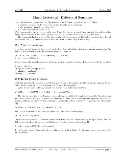
In a crude overview, we can say that Maple offers three different types of solutions to ODEs:
1. analytic solutions, in the form of an explicit formula for the solution;
2. the solution expressed as a series; and
3. a numerical solution to the ODE.
While an analytic solution may seem the most desirable solution, we must know that (similar to integration
where formal antiderivatives do not always exist) a nice formula for the solution may not exist.
The command dsolve is one of the most useful solvers in Maple as differential equations have lots of
applications, see [1, 2]. This lecture is a selection of the material in [3, Chapter 17].
27.1 Analytic Solutions
If we have no preference for the type of method, we just call dsolve without any special parameters. We
define y as a function of x by the following differential equation:
[> ODE := x*diff(y(x),x) = y(x)*ln(x*y(x)) - y(x);
[> s := dsolve(ODE,y(x));
Maple returns a formal solution where C1 is any arbitrary complex constant. How can we verify the solution?
[> yx := rhs(s);
[> syx := subs(y(x)=yx,ODE);
[> simplify(lhs(syx));
[> simplify(rhs(syx));
27.2 Taylor Series Methods
With this method, the solution is developed as a Taylor series and we use the conditions imposed by the
ODE to find values for the coefficients of the Taylor series expansion.
Let us look at the pendulum, defined by a second-order differential equation :
[> diffeq := l*diff(theta(t),t$2) = -g*sin(theta(t));
The l in the equation is the length of the pendulum, theta(t) is the angle measuring the deviation from
its vertical position and g is the gravitational constant. Since this is a second-order equation, we need two
initial conditions. At time t=0, the pendulum is in vertical position, so theta(0) = 0, and its velocity is some
v[0].
[> inits := theta(0) = 0, D(theta)(0) = v[0];
The ODE is thus defined by a differential equation and two initial conditions:
[> ODE := {diffeq,inits};
Observe the very important difference in the use of diff and D. In the equation, we set up a formula and use
diff. In the initial condition, we regard theta as a function of time and must use D.
[> sol := dsolve(ODE,theta(t),series);
To crank up the order of approximation, we change the variable Order. See the lecture on series to turn this
into a function.
Jan Verschelde, 19 March 2010 UIC, Dept of Math, Stat & CS Lecture 27, page 1

MCS 320 Introduction to Symbolic Computation Spring 2010
27.3 Numerical Solutions
Using numerical algorithms, we can study more advanced oscillators than just the pendulum. Let us take
the van der Pol equation: y ′′ − (1 − y 2 ) ∗ y ′ + y =0,withy(0) = 0,y ′ (0) = −0.1.
[> diffeq := diff(y(t),t$2) - (1-y(t)^2)*diff(y(t),t) + y(t) = 0;
[> inits := y(0) = 0, D(y)(0) = -0.1;
[> ODE := {diffeq,inits};
[> sol := dsolve(ODE,y(t),type=numeric);
[> sol(0.1);
We see that we get a list of three elements when we evaluate the solution at any given time. But if we are
only interested in the evolution of y(t) in function of time, we need to select from the output of dsolve the
right function for plotting purposes:
[> solfun := t -> rhs(sol(t)[2]);
[> solfun(0.1);
[> plot(solfun,0..20);
27.4 DEtools
The package DEtools offers a wide range of graphical tools to study ODEs:
[> with(DEtools);
Here we take the van der Pol equation again and make a “phase portrait” of two curves defined by the
equation. We first transform our second-order equation into a system of two first-order linear equations:
[> ODEs := diff(y(t),t) = yy(t), diff(yy(t),t) - (1-y(t)^2)*yy(t) + y(t)=0;
If we want to see two trajectories, we cook up two sequences of initial conditions:
[> inits1 := y(0) = 0, yy(0) = -0.1;
[> inits2 := y(0) = 0.1, yy(0) = 0;
[> DEplot({ODEs},[y(t),yy(t)],t=0..10,[[inits1],[inits2]]);
Jan Verschelde, 19 March 2010 UIC, Dept of Math, Stat & CS Lecture 27, page 2

MCS 320 Introduction to Symbolic Computation Spring 2010
27.5 Assignments
1. Show that the solution y(x) to the equation
a2 − y2 − a ln a + a2 + y2
+ a ln(y)+x = C
is a solution of the differential equation
2. Solve the following ODE:
and verify the solution you find.
3. Solve the following initial value problem:
y ′ y
= −
a2 − y2 .
3y 2 y ′ +16x =12xy 2
y ′′ − y =0, y(0) = 1, y ′ (0) = 0.
4. The Chebyshev polynomials Tn(x) satisfy the following differential equation:
(1 − x 2 )T ′′
n (x) − xT ′ n (x)+n2 Tn(x) =0.
(a) Apply dsolve to the differential equation and interpret what Maple returns to you.
Note: Tn(x) =cos(narccos(x)). (b) The command orthopoly[T](25,x) returns T25(x).
Verify that orthopoly[T](25,x) satisfies the differential equation.
5. Consider the following system of differential equations:
d
dtr(t) f(t)
=
=
1.1r(t) −0.75 f(t)
−
+
0.5 r(t)f(t)
0.25 r(t)f(t)
d
dt
r(0) = 3,f(0) = 2.
This system can be used to model the evolution in time t of two species, with f(t) thesizeofthe
predator population (f =fox)andr(t) the size of the prey population (r = rabbit).
(a) Use dsolve to define two numerical procedures rabbits and foxes which are functions of t:
rabbits(t) =r(t) andfoxes(t) =f(t), i.e.: rabbits is the solution for r(t) andfoxes is the
solution for f(t), as defined by the given system of differential equations.
(b) With these two functions, make a plot of the solution trajectories, for t going from 0 to 8.
References
[1] M.L. Abel and J.P. Braselton. Differential Equations with Maple V. Academic Press, second edition,
2000.
[2] D. Barrow, A. Belmonte, A. Bogges, J. Bryant, T. Kiffe, J. Morgan, M. Rahe, S. Kirby, and M. Stecher.
Solving Differential Equations with Maple V Release 4. Brooks/Cole Publishing Company, 1998.
[3] A. Heck. Introduction to Maple. Springer-Verlag, third edition, 2003.
Jan Verschelde, 19 March 2010 UIC, Dept of Math, Stat & CS Lecture 27, page 3