Long-Time Correlations in the Stochastic Regime - Charles Karney

Link: http://charles.karney.info/biblio/karney83c.html
Physica 8D (1983) 360-380
North-Holland Publishing Company
LONG-TIME CORRELATIONS IN THE STOCHASTIC REGIME
Charles F.F. KARNEY
Plasma Physics Laboratory, Princeton University, Princeton, New Jersey 08544, USA
Received 1 October 1982
Revised 1 February 1983
The phase space for Hamiltonians of two degrees of freedom is usually divided into stochastic and integrable components.
Even when well into the stochastic regime, integrable orbits may surround small stable regions or islands. The effect of these
islands on the correlation function for the stochastic trajectories is examined. Depending on the value of the parameter
describing the rotation number for the elliptic fixed point at the center of the island, the long-time correlation function may
decay as t -~ or exponentially, but more commonly it decays much more slowly (roughly as t -t). As a consequence these small
islands may have a profound effect on the properties of the stochastic orbits. In particular, there is evidence that the evolution
of a distribution of particles is no longer governed by a diffusion equation.
1. Introduction
Many important problems in physics are de-
scribed by Hamiltonians of two degrees of free-
dom. Examples are the motion of a charged par-
ticle in electrostatic waves, the motion of a charged
particle in various magnetic confinement devices,
the acceleration of a particle bouncing between a
fixed and an oscillating wall, the wandering of
magnetic field lines, etc. In such systems, there may
be a parameter k which governs the strength of the
coupling between the two degrees of freedom.
When k is zero (no coupling), the system is integra-
hie. As k is increased, some of the integrable
trajectories disappear, and the motion becomes
stochastic. Eventually, when the k is large, nearly
all of phase space is occupied by stochastic tra-
jectories. These properties are nicely illustrated by
the standard mapping [1]. Although this mhpping
is an idealization, it accurately portrays many of
the properties of real systems.
When k is small, various perturbation theories
are available to describe the trajectories approxi-
mately. On the other hand, in the highly stochastic
regime (k large) certain statistical quantities may
be analytically determined by assuming that the
0176-2789/83/0000-0000/$03.00 © 1983 North-Holland
motion is ergodic and that the correlation time is
short. In the case of the standard mapping, this
allows simple determinations of quantities such as
the diffusion coefficient [1, 2] and the KS-entropy
[1].
The purpose of this paper is to examine more
critically the assumption that the correlation time
is short in the stochastic regime. Our interest in this
problem was triggered by studies of the diffusion
coefficient for the standard mapping,
r,- r,_ I = - k sin 0,_1, 0,- 0,_l = r,. (1)
Far above the stochasticity threshold k >> 1, the
diffusion coefficient defined as
.~ = lira ((r,- ro) 2)
,~o 2t '
where the average is over some appropriate ensem-
ble, is given by assuming that 0 is a random
variable in the equation for r. This is equivalent to
assuming that the correlation function is propor-
tional to a delta function and gives the "quasi-
linear" result ~ ,~ ~ql = -Ik 2. Including the cor-
relations out to short times (about t = 4) gives

corrections to the diffusion coefficient reported by
Rechester and White [2] which can enhance the
diffusion coefficient by as much as a factor of
about two. However, a numerical determination [3]
of the diffusion at k = 6.6 gave ~/~ql ,~ 80. At this
value of k there is an island ("accelerator mode")
present in the stochastic sea. Although the orbits
used to compute ~ were all in the stochastic
region, they were able to wander close to the island
and stay close to it for a long time. This introduces
long-time correlations into the motion and ac-
counts for the anomalously large value of ~ ob-
served.
The appearance of islands in the stochastic
regime is not at all unusual. This may be seen from
Sinai's estimate [1] for the number v (T) of periodic
orbits of period ~< T: v(T) ~ exp(hT) for T--.ov
where h is the KS-entropy. Now the majority of
these periodic orbits are unstable. However as k is
increased, h generally increases (h ,~ log(~k) [1] for
the standard mapping) and hence new periodic
orbits must appear. Generally a tangent bifur-
cation is responsible for the appearance of the new
periodic orbits. At the tangent bifurcation, a pair
of stable and unstable periodic orbits is born. The
stable orbit gives rise to other longer periodic
orbits as k is increased and eventually becomes
unstable. Thus as we increase k, many small islands
appear via tangent bifurcations, survive for some
interval of k, and finally disappear (usually
through period doubling). If we pick a particular
value of k, it is not clear that there will necessarily
be any islands present. However, we may speculate
that at some arbitrarily close value of k, there will
be some islands.
It may be objected that the large effect seen in
the standard mapping arises because the islands
are accelerator modes [1] and that such islands are
a rather special feature of the standard mapping.
While accelerator modes are the only islands which
will contribute significantly to the force (i.e., accel-
eration) correlation function and hence to the
diffusion coefficient, any islands will contribute to
the correlation of some functions on phase space.
The results of this study will be applicable to
C.F.F. Karney ~Long-time correlations in the stochastic regime 361
systems like the Fermi map which have no acceler-
ator modes. This study also contributes to the
understanding of the more general problem of
motion in a divided phase space.
In this paper, we wish to examine more closely
the effect these islands have on a stochastic tra-
jectory. As far as determining the effect on the
correlation function, this involves determining how
"sticky" the island is. Given that the stochastic
trajectory comes within a certain distance of the
boundary of the island, how long do we expect it
to stay close to the island? This approach is
inspired by work of Channon and Lebowitz [4] on
the correlations of a trajectory in the stochastic
band trapped between two KAM surfaces in the
H6non map. Similar work has been carried out on
the whisker map by Chirikov and Shepelyansky
[5]. This work is being extended by B.V. Chirikov
and F. Vivaldi.
Since we concentrate only on the behavior close
to the island, this approach may be characterized
as a local one. This should be compared with
Fourier transform methods [2], which are global
and are not well suited to the description of
localized phenomena. For instance, Meiss et al. [6]
attempted to use such methods to compute the
long-time correlations for the standard mapping,
and they found poor agreement with numerical
experiments whenever islands were present.
The paper is organized as follows. In section 2,
we derive a canonical mapping which describes the
behavior near an island. Next (section 3), we define
the trapping statistics which describe how sticky
the island is. The results for the trapping statistics
are given in sections 4 and 5. In section 6, we show
how to apply these results to obtaining the cor-
relation function. The results are discussed in
section 7.
2. Derivation of mapping
Far into the stochastic regime for a general
mapping, the islands which appear via tangent
bifurcations are very small and exist only for a

362 C.F.F. Karney ~Long-time correlations in the stochastic regime
small interval in parameter space. This allows us to
approximate them by a Taylor expansion in both
phase and parameter space about the tangent
bifurcation point retaining only the leading terms.
This was carried out in ref. 3 where the resulting
mapping was reduced to a canonical form
Q: y, - yt- 1 = 2(xt 2- , - K) = g(x,_ 1; K) ,
Xt -- Xt- 1 = Yt "
Here K is proportional to k- k~n~ (k~,g is the
parameter value where the tangent bifurcation takes
place) and x and y are related to the original phase
space coordinates by a smooth transformation.
The mapping Q represents an approximation of
the general mapping close to the point of tangent
bifurcation. For K < 1, Q has no periodic orbits.
At K = 0, there is a tangent bifurcation when an
unstable fixed point appears at x = y = 0. (This is
not a hyperbolic point since its stability is deter-
mined by the quadratic terms in the mapping.) For
0 < K < 1, this fixed point splits into a pair of
stable (elliptic) and unstable (hyperbolic) fixed
points located at (x, y) = ( -T- x/~, 0), respectively.
The elliptic fixed point is usually surrounded by
integrable trajectories (KAM curves) which define
a stable region (the island) in which the motion is
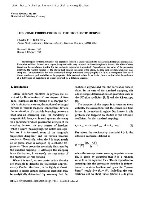
bounded. An example of island structure is shown
in fig. 1 for K = 0.1 (the value of K at which exten-
sive numerical calculations have been carried out).
At K = 1 the stable fixed point becomes unstable
and gives rise to a period-2 orbit via a period-
doubling bifurcation. At K = 1.2840 the period-
doubling sequence accumulates [7], and at this
point (or shortly hereafter [8]) the area of the stable
regions becomes very small. For 0 < K < 1, the
mapping Q may be transformed to the Hrnon
quadratic map [9], the parameter K being related
to Hrnon's cos • by
cos 0t = 1 - 2x//K
(ct is the mean angle of rotation for points close to
the stable fixed point).
(2)
0.4
o2
-o2 :")
- 0.4
-0.4 -0.2 0 0.2 0.4 0.6
x +.,/K-
Fig. 1. Some islands of the quadratic map Q (2) for K = 0.1.
Referring again to the islands shown in fig. 1,
consider a particle which at t = 0 is close to, but
outside, the islands. (We often speak of an orbit in
terms of the position of a particle whose equation
of motion is given by Q.) Initially, the particle will
stay close to the islands; however as we let
t~+ ~, we find (x,y)~(~, +_ o@. It is just such
trajectories we are interested in, because they cor-
respond to particles in the stochastic region of the
general mapping approaching the islands, staying
there for some time (and contributing to long-time
correlations), and then escaping back to the main
part of the stochastic region.
What we want to do is to follow such trajectories
numerically and see how long they stay close to the
islands. However, we need some method of fairly
sampling these trajectories. "Fairly" means that we
should sample them in the same way that a sto-
chastic trajectory of a general mapping does. Since
the stochastic trajectory is ergodic over the con-
nected stochastic region of phase space, we must
sample trajectories in the same way; i.e., we must
ensure that the superposition of all the sampled
trajectories covers the region outside the islands
uniformly.

We achieve this by changing Q so that the phase
space is compact. This may be accomplished by
replacing g(x; K) in Q by the periodic function
g*(x; K) = ~g(x; K) for x,,~. ~< x < Xm~x, (3)
[g(x +_ L;K) otherwise,
where L = Xm,, - x~, > 0. The resulting map will
be called Q*. If x~, and Xm~. are chosen to span
the region where there are islands in Q, then Q*
obviously will contain the same islands. Further-
more the motion close to the islands will be the
same. By replacing g by g*, the whole of phase
space becomes periodic in the x and y directions
with period L. The motion can be treated as
though it were on a torus. A particle which starts
near the island will, as with Q, spend some time
close to the island. But when it moves away from
the island it no longer goes to infinity, but rather
it loops around the torus and has another chance
to approach the islands. Since Q* is area-
preserving, this single orbit will ergodically cover
the region outside the islands in the desired man-
ner. Examples of such orbits are shown in fig. 2 for
the same parameters as for fig. 1. (One embarrass-
ing feature of Q* is that new islands are intro-
duced. They are in fact accelerator modes- a par-
ticle inside one of them loops around the torus in
either the x or y directions. As discussed in appen-
dix A, these islands do not effect the statistics for
the long trapping times.)
One useful way of looking at Q* is as a
magnification of a small region near a tangent
bifurcation in the general mapping. The difference
is that once the trajectory leaves the vicinity of the
islands, it is immediately re-injected on the other
side of the islands. In the general map, the tra-
jectory will spend some long time, which depends
on the ratio of the size of the islands to the total
accessible portion of phase space, in the stochastic
sea before coming back to the vicinity of the
islands.
Assuming that the long-time behavior of sto-
chastic orbits is dominated by the region close to
the islands, there are two advantages to reducing
C.F.F. Karney ~Long-time correlations in the stochastic regime 363
Y
Y
0.4
0.2
0
-0.2
-0.4
0.10
0.08
0.06
0.04
0.02
-0.4
-0.2 0 0.2 0.4 0.6
x + v"-ff
0
0.,50 032 0134 0.36 0.38 0.40
x + d-K
Fig. 2. (a) Stochastic trajectories for periodic quadratic map-
ping Q* for K = 0.1. (b) An enlar~ment of a portion of (a).
Here x~, + x/~ = - 0.4, xmx + ~/K = 0.6, X, = 0.02. (a) was
produced by plotting every 1000th point of 64 orbits each of
length l07 and (b) by plotting every 100th point of 64 orbits of
length 2 x 108.
the problem to a study of Q*. Firstly, since Q*
describes the behavior of most islands far into the
stochastic regime, the properties of many map-
pings may be treated by looking at a special
mapping Q* which depends only on a single
parameter K. The second advantage is that the
properties of orbits close to the islands may be

364 C.F.F. Karney ~Long-time correlations in the stochastic regime
studied much more efficiently because there is no
need to follow orbits while they spend a long and
uninteresting time far from the islands.
3. The trapping statistics
The prescription for numerically determining
the stickiness of the island system in Q is to
pick trajectories outside the islands in Q* and
to iterate the mapping many times. The mapping
is performed on the torus, i.e., x and y are reduced
_ ! L !L~
to their base intervals [Xmin, X,~x) and [ 2 ' 2 1
after each iteration. However, we keep track of
when an orbit moves off one edge and re-appears
at the opposite edge. The orbit is then divided at
those points when the orbit looped around the
torus, and the lengths of the resulting orbit seg-
ments are recorded. The main results of such a
calculation are then the trapping statistics f, which
are proportional to the number of orbit segments
which have a length of t.
Suppose that the total length of the orbit is T
and Nt is the number of segments of length t. If T
is so large that we can ignore partial segments at
the ends of the orbit (this problem is examined
below), then we have Y. tN, = T; the total number
of segments is N = E N,. The trapping statistics are
defined by ft = NJT and are therefore normalized
so that Y. ~ = 1. The mean length of the orbits is
given by at = 1~El (= T/N). The probability that
a particular segment has length t is p, = ~f,
(= N,/N). If an arbitrary point is chosen in the
orbit, then ~ is the probability that this point
belongs to a segment of length t and f is the
probability that it belongs to the beginning, say, of
a segment of length t.
Three factors effect the measurement off. They
are (a) the presence of the spurious accelerator
modes, (b) the choice of x~, and X~x, and (c) the
total length T of the trajectory used to measure f,.
The first two items only effect f, for small t (apart
from an overall normalization). In order to ac-
count for the last item, we define f, by
Nt/(T +1-t) (rather than Nt/T). This accounts
for the fact that we are less likely to observe orbit
segments whose length is close to T. All these
points are discussed in detail in appendix A.
The survival probability
P,= ~ PT (4)
~=t+l
is the probability that an orbit beginning in a
segment at t = 0 is still trapped in the same seg-
ment at time t. Note that P0 = 1 as required. This
is the quantity studied in refs. 4 and 5. The
correlation function
C,= ~ (t-z)ft= ~ P,/ot (5)
t=T t=T
is the probability that a particle is trapped in the
same segment at two times z apart. Again, we have
C0=l.
There are two other ways of interpreting C~. If
we start many particles at positions uniformly
distributed in the stochastic sea of Q* (i.e., in the
dark region of fig. 2), then C~ gives the fraction of
particles remaining in the L x L square after z
iterations of Q (rather than Q*). Alternatively,
consider a drunkard who executes a one-
dimensional random walk with velocity v =
dr/dt = + 1. The direction of each step is chosen
randomly, while the durations of the steps are
chosen to be the lengths of consecutive trapped
segments of Q*. Then for integer z, C~ is just the
usual correlation function for such a process, i.e.,
(v,v,+~),. The behavior of this random-walk pro-
cess is similar to the behavior of an orbit in the
general mapping when two accelerator modes with
opposite values of the acceleration are present.
(This is the case with the first-order accelerator
modes for the standard mapping.) In section 6, we
will show how C~ is related to the correlation
function for the general mapping.
A diffusion coefficient may be defined by
D = +co+ c,=y', 5t f,. (6)

This gives the diffusion rate for the drunkard in the
random-walk problem above. It is also related to
the diffusion coefficient for the general mapping
(see section 6).
Since Q* must be iterated many times to provide
good statistics for f, for large t, extraordinary steps
were taken to ensure that the numerical program
was fast and reliable. The time for one iteration on
a Cray-1 is a little less than 75 ns. One way that the
code was made more reliable was by doing the
arithmetic in fixed-point (as opposed to
floating-point) notation. The numerical mapping is
then one-to-one which is the discrete counterpart
of area-preserving. (Floating-point realizations of
mappings are typically many-to-one.) This pre-
cludes the possibility of an orbit, which starts far
from the island, approaching the island and be-
coming permanently trapped near the island. Even
though such behavior is forbidden for an area-
preserving mapping, it may be observed with a
floating-point realization. Details of the numerical
methods are given in appendix B.
4. The results for small K
We begin by considering the cases where K is
small or zero. In this case the mapping equations
are nearly integrable and this enables us to derive
approximate analytic expressions for f,. Fig. 3
showsf~ for K = - 10 -4, 0, and 10 -4. Three types
of behavior are seen for t --* oo: a cutoff distribution
f~ = 0 for t > t,~, ~ 50, a rapid algebraic decay
f,~t-7, and an exponential decay f,
exp(- 0.1 t ).
The easiest case to begin with is K = 0. The
method for deriving f, analytically consists of
computing the length of the trajectory through
some point and then assigning some probability
that this trajectory will be chosen. The first part of
the calculation has been carried out by Zisook [10].
We repeat the calculation here to establish the
method for other cases.
When K = 0, we are exactly at the tangent
bifurcation point. There are no islands in this case,
C.F.F. Karney / Long-time correlations in the stochastic regime 365
f[
-2
I0 ~-
16 K:
, il - \ o,
16 s
IO' .
i-]
~o -3_
-6
I0
-9
I0
tO -,2
16 Is
i0 "z _
10 -4 _
i() 6 --
i(~ II _
i(~ I° _
16 Iz
0
. . . I
01 3 5 tO z
t
exp~O.It),,,, [ ,
.
I
i01 I0 2 IO s
t
K=I04
50 I00 150 200
Fig. 3. The trapping statisticsf~ for (a) K = ~ b ) K = 0,
and (c) K= 10 -4. In each case x~o+x/max(K,O)=-0.5,
xw,+~=0.5, Xr=0.02. For (a) M = 128, q = 1,
qT = 5 x 107; for (b) and (c) M = 512, q = 2, qT = 108. In (b)
and (c) the straight lines give the t -7 and exp( -0. It) behaviors
predicted in section 4.

366 C.F.F. Karney / Long-time correlations in the stochastic regime
but trajectories can still spend arbitrarily long near
the fixed point at (x,y)= (0, 0). Near this point
x, - xt_ 1 and Yt - - Yt- ~ are small. We therefore
rescale x, y, and t with x = ,~X, y = EaY, t = E -IT
where E is small. The mapping Q becomes
Y(T) - Y(T - E)
E
X(T)-X(T-E)
E
= E 2#-~- '2X2(T -- E),
= E.-~-l Y(T).
Choosing ct = 3 and fl = 2 and replacing the left
hand sides by derivatives, we obtain
dY dX
-- = 2X 2, - y.
dT dT
These are Hamilton's equations (with X and Y
being conjugate position and momentum coordi-
nates) for the Hamiltonian
H - ! v2 _ _2.y3 (7)
-- 2 ~ 3 ~ "
Curves of constant H in the (X, Y) plane give the
trajectories, examples of which are shown in fig.
4(a). We define the trapping time as the time it
takes to traverse one of these curves from
Y = - ~ to oo. (This Hamiltonian gives escape to
infinity in a finite time. The time taken for a
particle to escape to infinity in Q is infinite, but
very weakly so. The particle reaches y from y = 0
in roughly log logy steps for y large.) Since
dX/dT = Y = x//-2(H + 2X3), the trapping time
may be written as
i dX
T(Xo) = 2 %/4(X3 _ X3 ) ,
x0
where X0 =- (~H) 1/3 is the X intercept of the
trajectory with Y = 0. Performing the integration
gives
T(Xo) = f 3t x
rX O.
Y
Y
4-
2
0
-2-
-4-
4-
3-
2
0
-3 -2 -I 0 I 2 3
X
-3 -2 -I I 2 3
X
Fig. 4. Trajectories, for the Hamiltonian with (a) K = 0 (7) and
with (b) K small and positive (11). In both figures H takes on
equally spaced values with an increment of 4.
(The numbers here may be written in terms of
incomplete elliptic integrals.)
This completes the computation of the trapping
time. We now assign weights to each trapping time
by requiring that particles spend equal times in
equal areas of phase space. Let A (X0) be the area
between the trajectory passing through the origin
and that passing through (X0, 0) in fig. 4(a). Since
Y ~ X 3/2, scaling invariance gives A (X0) =
A(1)X~/2. (This procedure needs to be carried out
separately for positive and negative X0. However,
• the scaling relations are the same in the two cases.)

Parameterizing in terms of the trapping time T
gives A(T),~ T -5. The fraction of particles which
are trapped for times between T and T+ dT is
proportional to the differential area dA(T)~
T- 6 d T. Finally, we divide by T to give T- 7 d T as
the number of orbit segments of lengths in this
range. In unsealed variables, we have f ~ t-7
which is valid for t large. The correlation function
has the asymptotic form C, ~ z- 5
It is interesting to enquire what the asymptotic
behavior for f would be if g in (2) were a higher-
order polynomial in x. Ifg(x; 0) = x", with m > 1,
we can repeat the above calculation and find that
ft " tO m + l)/(ra - 1) "
1
Since f, has a finite second moment, D always
exists. (For m = 1, we find an exponential decay of
f,. This corresponds to the case K > 0 discussed
below.)
When K is small and negative, there are no
periodic orbits. The particle can spend only a
bounded time close to the origin. Defining scaled
variables as before, together with K = -E 4, gives
differential equations which are derivable from the
Hamiltonian
H =½Y2 2 3
- ~X - 2X. (8)
The trapping time is now
T(X0) = i
xo
dX
,,/~x ~ + x - kXo 3 - Xo'
where X0 is the X intercept of the trajectory with
Y = 0, i.e., it is the real root of H + 2X03 + 2X0 = 0.
This is plotted as a function of X0 in fig. 5(a). We
see it attains a maximum value of Tr~x = 5.1454 at
Xo=-0.5536. In unsealed variables this means
that the maximum trapping time is tm~=
5.14541KI -I/4 and that this trapping time is at-
tained by particles passing through (x,y)=
(-0.5536 Iv/~, 0). The Ig[-" scaling of the max-
C.F.F. Karney ~Long-time correlations in the stochastic regime 367
(9)
o
u_
6 I ~ I
5-
4
3
i
2
i
r f l I
-10 -5 0 5
×o
10 6 __.
10 5
10 4
10 3
!0 2
i01
(o)
t , r ~ r , w r
(b)
I I I "-¢1 I I I I
2
3 4 5 6 7 8 9 I0
Fig. 5. (a) The trapping time T(Xo) for K < 0 (9). (b) F(T) as
a function of T (10).
imum trapping time has been derived by Zisook
[10].
To assign probabilities to the various trapping
times, we define A(Xo) as the area between the
trajectory passing through (0, O) and that passing
through (Xo, 0). Since Y = 2x/~X 3 + X - ½X0 3 - X0,
we obtain
oo
A (Xo) = 4 f ~/lx~ + x dx
0
- 4 ~/lx 3 + x - ~Xo - Xo dX.
xo
T

368 C.F.F. Karney / Long-time correlations in the stochastic regime
(The two integrals need to be done to together to
get a finite answer.) Differentiating gives
dA (Xo)/dX o = 2(X 2 + 1)T(Xo).
The number of orbit segments of length T is then
proportional to
1 dA(Xo)/ldT(Xo) 2(X2+ 1)
F(T) =_ fr ~00 /1~ = E Ir'(Xo)l
(lO)
The right hand side is written as a function of X0.
This is converted to a function of T by inverting
T(Xo). Since this gives a double-valued function,
the two branches must be summed over as indi-
cated by the summation sign. In unscaled variables
we have
f, ,~ p(lgll/4t)
for t = ¢(IKI- 1/4). The function F(T) is plotted in
fig. 5(b). For T ,~ Tmax, we have F(T) ,,~ 6.205 ×
10ST -7 while for T ,~ T~_~, F(T) ,~ 3.024 x
(Tm~x - T)- 1/2. The correlation function is given by
the second integration off, so that for T ,~ tr~ we
have C~ ~ (/max- ,~)3/2 for z ~< tmax-
Fig. 5(b) should be compared with fig. 3(a). The
effect of the singularity in F(T) at Tmax is evident,
although its position isn't quite right. Further-
more, the decay off, for smaller times is somewhat
slower (approximately as t -6) than for F(T). These
discrepancies arise because we are not far enough
into the asymptotic regime since E is not very small
(0.1). The formula t~x = 5.1454[K1-1/4 may easily
be verified for smaller values of [K I. The T -7
behavior of F(T) has of course the same origin as
that off, for K = 0. However, the numerical results
for K = 0 given in fig. 3(b) show that it is not
attained until about t ~ 100. When K = -10 -4,
tm~x is only about 50, and there is no interval in
which the t-7 behavior is exhibited.
Finally we turn to the case K > 0. As with
K < 0, we can approximately derive the motion
from the Hamiltonian
H = ½ y2 _ 2X3 + 2X, (11)
where we have used the same scaled variables as
previously except that K = e 4. The trajectories for
this Hamiltonian are given in fig. 4(b). There is
single island centered at the fixed point at
(X, Y) = (- 1, 0) and the island extends all the way
to the separatrix emanating from the unstable fixed
point at (X, Y)= (1,0). This is an idealization
because for the mapping there is a stochastic band
close to the separatrix. However, for small K this
band is very thin, and the island does have quite
a "clean" outer edge.
We may carry out the analysis given for K < 0
with appropriate changes to obtain f' analyticall~y.
However, we may avoid doing a lot of tedious
integrals by concentrating only on the long-time
behavior of f'. For shorter times, namely for
lO0

The area A (40) between the hyperbola, the axes,
and the lines ~ = 1 and r/= 1 is
A(¢o) = ~2(1 -- 2 log ~o).
The trapping statistics are then given by
I dA
f, "~ t dt "~ exp(- t log 2t).
For the fixed point at (0, v/K),
/
2 = 1 + 2x/'K + 2Jx/~ + K ~ 1 +
f, ~ exp( - K~/4t).
C.F.F. Karney ~Long-time correlations in the stochastic regime 369
2KI/4 '
C~ behaves in the same way. For K = 10 -4, the
decay rate should be about 0.1, which is indeed
what was observed in fig. 3(c). Similar agreement
is seen at K = 10-3 and 10 -2. However, at K = 0.1,
the central island has shed a chain of sixth-order
islands and the foregoing analysis does not apply.
This case is discussed in the next section.
5. The results for K = 0.1
We have measured f` for K between 0 and 1.3 at
intervals of 0.05, and at most of the values of K a
slow algebraic decay off, is seen. A representative
case is K = 0.1, whose trapping statistics are given
in fig. 6(a), which illustrates the slow decay for very
long times t ~ 107. Also given in fig. 6 are Pt, C,
and ~t = -d log Cffd log z (thus locally CT ~ z- ~).
This last plot shows the power at which C~ decays
varying between about ¼ and 3.
A glance at fig. 2 shows the origin of this
behavior. The central island is surrounded by a
chain of sixth-order islands. Around each of these
islands are several other sets of islands. This pic-
ture repeats itself at deeper and deeper levels. A
particle which manages to penetrate into this maze
can get stuck in it for a long time.
For z ~< 10 4, fig. 6(d) gives ~t ~ ~. Correspond-
ingly we have P, ~ t -p where p = 1 + ~t ~ ~. This is
close to the asymptotic (t~oo) result found in ref.
5 for the whisker map, in which (p) ~ 1.45. This
is another indication that the behavior of a Ham-
iltonian with a divided phase space has "universal"
properties. However, in our case, 0t shows some
strong variations beyond z ~ 104 where CT "steps
down" (e.g., between 10 4 and 3 x 105). This means
that the asymptotic form of C~ is very difficult to
determine numerically.
The diffusion coefficient D is given by the sum-
mation of C and is approximately 6400 _+ 800. The
error is estimated by calculating D separately for
subsets of the orbits sampled. Unfortunately, be-
cause a few very long orbit segments have such a
large effect on D, the individual observations of D
come from a highly skewed distribution and the
error may be severely underestimated. We will try
to get an idea of the error by asking what behavior
is possible for f` for ta = 108 < t < 2 x 10 9 = I b (l b is
the length of the orbits used to compute f, in fig.
6). Since no segments were observed in this range,
we have
tb
f M(tb- Oft dt >ta and ~>0, we can
evaluate the integral to give MAtatb/(1 + or) ap-
proximately. If we take A = 10 -20 (this value was
estimated from fig. 6(a)), we find 0t ~> 2. In the case
of the slowest decay, ~ = 2, the portion of f`
between ta and ~ would increase D by about a
factor of 2 over the value given above. If f` takes
another step down near t = l0 s, then A might be
smaller and smaller values of'~ would be possible
and the maximum error in D would be larger. For
instance with A = 0.3 x 10 -2°, then all values of
ct > 0 are consistent with the numerical obser-

370 C.F.F. Karney / Long-time correlations in the stochastic regime
iO 4
i0 "8
i0 -12
'%
i0 ~16 _
(o)
L ! L __~ 16 6
I02 104 I0 s i0 B
[ ~ ' I ' I ' I '
i 10 -9
i(~121 , I , l * i , "~
I 10 2 10 4 10 6
f
iO B
_o
C r
ji.o
20
1.5
0.5
0
' ' {c)
I , I , I i
rO 2 i04 tO e 10 8
, i , ~ , l ,
10 2 10 4 I0 6 10 8
Fig. 6. (a) The trapping statistics f, for K = 0.1. (b), (c), and (d) show P,, C,, and d log CJd log z for the same case. Here x~, +
x/~ = - 0.4, Xma x + x//K = 0.6, X, = 0.02. The data for f, was obtained in 3 pieces; for 1 ~< t < 103, M = 128, q = 1, qT = 5 x 107;
for 103 x< t < 105, M = 256, q = 10, qT = 5 × 108; for 105 ~< t, M = 1600, q = 1000, qT = 2 x 10 9.
vations. Since C~ sums to infinity for all ~ ~< 1, D
may well be infinite!
If D is indeed infinite, we would wish to know
how a group of particles spreads with time. We
again consider the drunkard's walk based on Q*
which was introduced in section 3. The second
moment of r is related to the correlation function
by
S, =- ((r, - r0)2> = tCo + 2 ~ (t - z)C~. (12)
This is plotted in fig. 7(a), using the data of fig. 6.
For t ~< 104, S t grows somewhat faster than 13/2 (see
fig. 7(b)) and even until t ~ 107, St is growing
significantly faster than linearly. Beyond 107 , the
numerical data shows a convergence to a linear
rate; but this is merely because no segments longer
than about 6 x 107 were observed. For t--*oo, St
grows as t 2-=, assuming that the exponent 0t at
which C~ decays asymptotically is less than 1. If the
diffusion coefficient is estimated from D, = lsJt,
then D, grows with t as shown in fig. 7(c).
When applying these results to the general map-
ping, we will need to know the area b2 occupied by
the stochastic trajectories (the dark area in fig. 2).
This was calculated by dividing the phase space
into 1024 x 1024 little boxes, iterating the mapping
many times, and counting the number of occupied
boxes. It is important to iterate the map enough
times so that (a) the expected occupation number
of each box is reasonably large and (b) the tra-
jectories have time to wander into all the nooks
and crannies. (In practice, the second requirement
is more stringent.) With x~,, x~, and X, as given
in the caption to fig. 6, the area of the stochastic
component is found to be about b2 = 0.693.

7.
o
10 '2
i09
106
i03
C.F.F. Karney / Long-time correlations in the stochastic regime 371
] r I J
I I I i
102 104 t I06 108
l~ ~ l ~ , ,
I I02 104 t [06 108
[04 l l
i0 3
,~- 102
I0
(c)
I I
I02 i04 I06 i08
t
Fig. 7. (a) The variance S, for the case given in fig. 6. (b) and
(c) show d log Sfld log t and D, = ½SJt.
6. Application of the results
We wish now to determine the contribution of
an island to the correlation function of an orbit in
the stochastic component of phase space of a
general two-dimensional area-preserving mapping
G. (The analysis applies equally well to Ham-
iltonians with two degrees of freedom. The phase
space is then the Poinear6 surface of section and
the unit of time is the period of the island.)
For simplicity we begin by considering the case
where there is a single small island embedded in the
connected stochastic component. Let the total area
occupied by the stochastic component be Am. Sup-
pose a small island centered at x0 is immersed in the
stochastic sea. When iterating Q*, we have been
approximating G in small region around x0. The
square defined by x~n and Xm~ in Q* is trans-
formed into a small box (parallelogram) of area B0.
The ratio of the areas in the two spaces is
Bo/L 2 = ?. Suppose the area of the stochastic com-
ponent of G which lies inside this box is B1. (In the
notation of appendix A, Bi = ?bl.) Recall that Q *
also contains spurious islands (accelerator modes)
which have no counterpart in G. To account for
these islands we define f* as in (A. 1). From this we
can derive E f* = 1/~* and p* = 0t'f* (paralleling
the definitions made in section 3).
It is useful to begin by forming an idea of what
a stochastic trajectory will look like. Orbits will
consist of alternating trapped and free segments.
The trapped segments are those which are re-
stricted to B1, while the free segments are those
excluded from B~. (Here and in the following we
use B1, etc., to refer to a particular subset of phase
space as well as the area of this subset.) The basic
assumption is that each visit to the island is
uncorrelated with the previous one. So, on first
entering the area B~, we assume that a segment of
length t will be chosen randomly with probability
p*. A simple model for the motion in the stochastic
region Ai -- Bi, which excludes the region near the
island, is as follows. The first point after a trapped
segment is randomly (and with a uniform distribu-
tion) situated in A~- B~. This is in accord with
the picture that once an orbit leaves B~, it rushes
away from the vicinity of BI extremely quickly. If
this point is the pre-image under G of BI, then the
next point is the first point of another trapped
segment. Otherwise another point is chosen at
random in A~ - B~ and the procedure is repeated.
The mean length of trajectories trapped in B~ is 0t*.
The area of the points which are initial points of
trapped segments is therefore BliP*. These are the
points whose pre-images lie outside Bl- Thus the
probability that a point in A~- BI is a pre-image

372 C.F.F. Karney ~Long-time correlations in the stochastic regime
of BI is E = (B~/~*)/(A~ - BO. The probability that
a particular free segment has length t is then
E(1 - E) t- ~. These probabilities ensure that ratio of
time that the trajectory spends in Bt and in A~ - B l
is in the ratio of the area of these regions. (The
assumptions made to obtain the distribution of
lengths of the free segments is probably overly
restrictive. However, such a "memory-less" model
is probably accurate for the long times we are
interested in.) This model is discussed in more
detail in appendix C where it is used as a basis for
constructing a Markov-chain approximation of the
motion.
Consider the correlation function
cg(z) = (h(x(t))h(x(t + z))>t, (13)
where h is some smooth function of the position in
phase space x (in particular we require that it is a
constant throughout B 0. We shall assume that the
mean value of h(x(t)) is zero for the stochastic
orbits. We identify those terms in (13) for which
x(t) and x(t +z) belong to the same trapped
segment as ~s(z) the contribution to cg(T) due to
the island. (Thus for such terms we have
x(t + *')eBl for all z' such that 0 < z' ~< z.) Except
for z = 0, the other terms are smaller by a factor
of about BI/A1, which is typically very small. This
is so because h has a zero mean and because of the
rapid mixing of orbits in A 1 -- B|. This question is
examined in appendix C where it is also shown that
the additional terms do not contribute to the
diffusion coefficient, c£~s(z) may be written as
cgi~(r) = h2(x°) A~ t=, ~ (t-r)f*.
The first factor arises because both endpoints are
in B~ and h(x) ~ h(x0) for such points. The second
factor is the probability that x(t). lies in BI, and the
sum is the probability that x(t + z) belongs to the
same trapped segment as x(t). This sum is just the
correlation function defined in terms off* instead
off, For large z, we can substitute for f* using
(A.2), and the sum becomes (bJbOC~. Thus the
contribution to the correlation function due to the
island is
c~is(z) = h2(x°) A~ b2C,.
Equation (A.3) shows that this result is indepen-
dent (for large z) of the choice of Xm~x and x,~,
(which is as it should be).
If h is the rate of change of one of the com-
ponents of x, e.g., h(x)= dx/dt, then the island
enhances the x-space diffusion coefficient by
~is = h 2(xo) -~l b2D ,
where D (assuming that it exists) is given in (6).
Whether or not D exists, the mean squared x
position of a group of particles initially concen-
trated in a small region is enhanced by
2~ais(t) = h2(x0) ~ bzSt,
where S, is given by (12).
If there is more than one island, then the
contributions should be added together in ~, and
9. If there is a chain of Nth order islands at
x0, x~ ..... xu = x0, their contribution to the cor-
relation function ~g(Nz +j) is
N-I
cg~(Nz +J)= ,=0 ~ h(x')h(xi+J)-~tbzC*'
where ?--BolL 2 for one of the islands and
0 ~

k = 2nn (n an integer) [1]. The acceleration in such
a mode is r t - rt_ ~ = _+ 27rn. These modes appear in
pairs, one with each sign of the acceleration. We
will take the area of the stochastic component A~
to be equal to the entire area of phase space (2rr)2.
The relation between the parameters is found by
matching the residues at the stable fixed point. This
gives k 2 = (2nn) 2 + 16K. when transforming to the
quadratic map Q, lengths are magnified by a factor
lrm [3] and so y = (2/Trn) 2. If we wish to estimate
the diffusion coefficient, we must define h to be the
acceleration; thus h(x0)= + 2zrn. For K = 0.1, we
take b 2 = 0.693 and the proportionality constant
connecting the scripted and unscripted quantities
above is 2h2(xo)(y/AOb2 ~0 0.56. (The factor of 2
accounts for the presence of the two islands.)
Using ~ql = (nn) 2 and taking 6400 as a lower
bound for D, we find that the contribution to the
diffusion coefficient is increased over its quasi-
linear value by a factor of at least 360/n 2. Thus for
n = 1 or k ~ 6.41, the islands completely dominate
the diffusion. The first-order accelerator modes
continue to have such a large effect at least until
k ,~ 100. If D is in fact infinite, even arbitrarily
small accelerator modes will eventually dominate
the motion and fig. 7 can be used to estimate the
time at which the accelerator modes become im-
portant.
7. Discussion
We have looked at the effect of a small island on
the correlation function for the stochastic tra-
jectories of Hamiltonians of two degrees of free-
dom. When the parameter K is small, the problem
may be treated analytically and we find that the
contribution to the correlation function C, is zero
for z ~> 5.1454[K[ -~/4 when K 0.
The more interesting case is when K is not small
and the island is surrounded by other islands. In
the case we considered in detail K = 0.1, the decay
of the correlation function is algebraic and very
C.F.F. Karney / Long-time correlations in the stochastic regime 373
slow (roughly as • -~) out to times on the order of
"t ~ 107. Even when the islands are small, this can
still lead to an enormous increase of quantities
such as the diffusion coefficient. Although it has
not been definitely established, there are strong
indications that the diffusion coefficient may be
infinite, indicating that the distribution of particles
does not obey a diffusion equation and that the
particles spread more rapidly than diffusively. Such
behavior is fairly typical, having been observed at
several other values of K.
It would be interesting to know how the distri-
bution of particles does evolve in time. If we
consider a system like the standard mapping at a
parameter value for which an accelerator mode
exists, then for large t this distribution could, in
principle, be found from f,, but its determination is
beyond the scope of this work. For now, we
observe that the distribution will be far from
Gaussian for times at least until t = 108. It will
contain a very small but extremely long tail that
contributes significantly to the variance. This has
important consequences for numerical experi-
ments. Imagine trying to measure S, for t = 108 by
directly measuring r,- r o for N particles. If N is
merely some "reasonably" large number like 1000
then S, will most likely be greatly underestimated.
(To counteract this there is a tiny probability that
St will be fabulously overestimated.) We know that
we should sample some orbits with r, - r0 ~ 107 to
be able to estimate St accurately. But since St ~ 104,
we need to sample at least (107)2/104= 10 l° orbits
before the effect of such a long segment is correctly
diluted. Obviously such a calculation is totally out
of the question. A much better approach is to
measure the correlation function and to derive St
using (12). On the other hand, the requisite number
of orbits probably are sampled in real experiments.
For instance in plasma physics applications the
total number of orbits is typically 1014 .
There are several questions still to be answered.
What is the long-time behavior of the correlation
function? Fig. 6 shows that it has not attained any
well-defined asymptotic limit by z = 107. What
determines the asymptotic behavior of the cor-

374 C.F.F. Karney ~Long-time correlations in the stochastic regime
relation function? The simplest picture we can
form for treating this problem would go something
like this: There is some outer KAM curve marking
the boundary of the main island centered at
( - x/K, 0). According to Greene [11], this curve is
approximated from the outside by a sequence of
islands whose winding numbers are the rational
approximants to the irrational winding number of
the KAM curve. Thus the long time behavior off'
may be found by considering how an orbit wanders
through these islands to approach the KAM curve.
Greene [12] found an algebraic decay of the cor-
relation function based on a simple model of such
a process. Equivalently this behavior may be ob-
tained from a diffusion equation in which the
diffusion coefficient approaches zero sufficiently
fast as the KAM curve is approached. This picture
was the one proposed in ref. 5.
Such pictures are however probably incomplete.
There is no reason to suppose that the KAM curve
around the central island determines the asymp-
totic behavior off,. For K = 0.1, it could equally
well be the last KAM curve around the sixth-order
islands which surround the central island, or the
KAM curve around one of the chains of islands
around the sixth-order islands, or all of them
together! For instance, the longest orbit segment
seen for K = 0.1, whose length was about 6 x 10 7,
spends most of its time around such a chain of
islands whose order is 6 x 23 = 138. (One of the
members of this chain is visible in fig. 2(b) at
x + x/~ ,~ 0.352 and y ,~ 0.034.) Is it the KAM
surface around this island chain that will determine
the asymptotic behavior off'? In this picture, the
asymptotic behavior is determined by the islands at
a finite depth in the islands-around-islands hier-
archy. This may be false. Perhaps as t is increased,
we must look at deeper and deeper levels of the
hierarchy. Such is the view taken by Chirikov in
ref. 13. We may also have to jump between
branches of the hierarchy as t increases. (This is
supported by the observation that the three longest
orbits seen for K = 0.1 are each stuck close to
different island chains.)
The absence of any idea as to the asymptotic
behavior of C, makes it virtually impossible either
to obtain numerically an upper bound on the
diffusion coefficient or to establish that it is un-
bounded. Such questions can probably only be
answered when this problem is better understood
analytically. In any case, it may be necessary to
take a critical look at extraneous effects which act
as an extrinsic noise source and which will cut off
the very long correlations.
Finally, what is a measure of these islands? This
gives the overall importance of this phenomenon.
We already have Sinai's estimate as to the number
of islands that will be created. What is still needed
is some estimate of their size and of the interval in
parameter space in which they exist. Numerical
evidence suggests that these both decrease rapidly
with the period. The latter quantity would enable
us to say what is the measure of parameter space
on which we expect to see islands.
Acknowledgments
This work was supported by the U.S. De-
partment of Energy under Contract DE-AC02-76-
CHO3073. I began it while at the Institute of
Plasma Physics, Nagoya University, participating
in the U.S.-Japan Fusion Cooperation Program.
Some of the work was carried out while at the
Aspen Center for Physics. I would like to thank
J.M. Greene, R.S. MacKay, and F. Vivaldi for
stimulating discussions. B.V. Chirikov provided
some enlightening comments on a preliminary
version of this paper.
Appendix A
Properties of the periodic mapping
In order to obtain correct trapping statistics, we
would like to uniformly sample the trajectories the
area outside the islands of Q and measure how
long each trajectory spends close to the islands. We
achieve this goal by looking at long trajectories of
Q*. In this case, "close" is determined by Xr~, and

x~a~. However, fig. 2 shows that the area outside
the islands is not sampled uniformly. There are
holes in it corresponding to the spurious islands.
Suppose that the order of a particular set of islands
is n. Particles in this set of islands will have looped
around the torus at least once in the x or y
direction after n iterations of Q*. (These islands
are accelerator modes.) A trajectory of length n
within these islands is made up of one or more
segments. It cannot be part of a longer segment. By
omitting the trajectories within the islands we are
therefore undercounting the segments with lengths
less than or equal to n.
We can express this in a more quantitative way.
The total area of phase space in Q* is b 0 = L 2. We
define bj to be that part of b0 which is not occupied
by the islands of Q and b2 to be the area of the
stochastic component of Q*, i.e., that part of b0
which is not occupied by the islands of Q*. The
difference between these two, b~ - b 2 gives the area
of the spurious islands. To include the effect of the
spurious islands, we define f* by
bl - b2 g, (A. 1)
f* = ft + bl '
where gt is the contribution from the regions of
phase space occupied by the spurious islands. If g,
is normalized like f, to have a first moment of
unity, then f* has the same normalization. The
factors multiplying f, and g, are just the relative
areas of those regions of phase to which these
trapping statistics apply. Now gt specifies the
lengths of orbit segments in the spurious islands,
which must be less than or equal to nm~x the
maximum period length for these islands. Thus gt
is zero for t > nma~. If we wish to calculate C~, we
need only know the trapping statistics for t > z. So
as long as z > n .... we may ignore g, and use
b2
ft* = ~f,. (A.2)
ol
These spurious islands have one other inter-
esting effect. They introduce correlations between
C.F.F. Karney / Long-time correlations in the stochastic regime 375
the lengths of successive segments. Consider an
orbit close to such an island chain of period 3.
Then, in the simplest case, we expect to see a
succession of segments of length 3. Such cor-
relations are obviously a peculiarity of Q*. In the
general mapping, where the particle spends some
time in the stochastic sea before returning to the
neighborhood covered by Q*, the trapped seg-
ments will be sampled randomly.
We next examine the effect of the definition of
"close," i.e., at the effect of changing x~ and Xmax.
Consider the effect of increasing the box size by
decreasing x~, and increasing Xmax. This has two
effects: new segments which never entered the
original box appear; and all the original segments
may be extended both forwards and backwards. As
long as the original box was large enough, the new
segments will all be short (since they never get close
to the islands). By the same argument, the exten-
sion of the orbit segments will be small. Because of
the extremely rapid departure of orbits away from
the islands, we can, for instance, double the edge
of the box and only increase the average length of
the orbits segments by less than one. So the main
effect of increasing the box size will be to increase
the number of short segments. As in the case of the
accelerator modes, we can quantity this. If we
change x~, to x~, and x~ to X~ax, then, for large
enough t, the new trapping statistics f; are given by
b~f; = bj,, (A.3)
where b~ is the area of the stochastic component in
the new box.
Lastly, we address the problem of estimating the
trapping statistics from an orbit of length T.
Consider an infinitely long time record consisting
of segments of various lengths t = 1,2 ..... Pick a
random record of length T and call N, the expected
number of segments of length t. (We do not count
partial segments at the ends.~ Then
0 for t > T,
Nt= (T+l-t~ for0

376 C.F.F. Karney ~Long-time correlations in the stochastic regime
This may be proved by induction. When T = 0, we
have Aft = 0 as required. When we extend the
record from T-1 to T, the only way a new
segment of length t can be included is if the particle
is at the end of such a segment at time T. Because
the probability of this happening is f~, N, increases
by f, for t

will remain zero. Thus there will be n = (248-m) 2
points accessible in the unit square. (Typically
m = 2 and n ,~ 1027.)
We are now ready to give the procedure for
gathering the trapping statistics f,.
(1) Read in K, x~,, x~, X,, T, q. (The trapping
statistics will be collected for the qth power of
the mapping. Tis the total number of iterations
of N -q. X~ defines the size of the randomizing
zone.)
(2) Initialize B,.~0 for 0 I_X].)
(7.2) Set Y¢--Y- G(X) where G(X) is calculated
as outlined above. If I_Y] #0, set P~true.
Set Y~ Y - [_Y_J. Return.
The bin number b(t) is defined by
C.F.F. Karney ~Long-time correlations in the stochastic regime 377
b(t) =
t for t ~< 50,
130 log10 t] for 50 < t < 105 ,
150 for 105 ~ t.
Finally the trapping statistics f, are obtained by
{ B/(T+ l-i) for i ~< 50,
Fi = Bi/( T + 1 - 100 +1/2)/3°) otherwise
V 10

378 C,F.F. I(arney / Long-time correlations in the stochastic regime
straightforward implementation in FORTRAN using
floating-point arithmetic. The most time-
consuming computations were those of fig. 6 where
M = 1600 orbits of length qT = 2 × 109 were used,
a total of 3.2 x l0 n iterations of N. This consumed
about 65 hours of cPu time on the Cray-1.
Aside from the computation of G(X), all the
calculations are exact. N is therefore area-
preserving, or, since only a discrete set of numbers
may be represented on the computer, it is better to
say that it is one-to-one. A trajectory may be run
backwards by
N -I = j-1Ntj,
where J is the involution (j2 is the identity)
J: X,=Xt-I- Yt-1+½ (modl),
Y,= - Y,_~ (mod 1)
which may be calculated exactly using fixed-point
arithmetic.
Because of the discreteness of the number system
on a computer, all the trajectories of a numerical
mapping are eventually periodic. Because N is a
one-to-one mapping, the whole trajectory will be
periodic. There will be no initial transient. Pre-
sumably the typical period length of an orbit in the
stochastic part of phase space is very long. Rannou
[14] gives ½(n + 1) as the average length of a
trajectory in a random permutation of n points.
(This is to be compared with the period length for
an orbit in a random function on n points which is
+ ~ approximately [15]. The distinction be-
tween a function and a permutation is that a
permutation is a one-to-one mapping of the n
points onto themselves, while a function is a
many-to-one mapping of the points into them-
selves. It is not clear whether the stochastic orbits
of floating-point mappings are closer to those of
random permutations or random functions.) How-
ever, N is not a random mapping because it
possesses symmetries. In the case of the standard
mapping this reduces the expected length of sto-
chastic orbits to d~(x/~) [14]. Although this number
"is still large (about 10~3), we expect there to be a
large number of trajectories with shorter periods.
Examples of such trajectories are those in the
accelerator modes which are restricted to a small
fraction of phase space. By composing the map-
ping with R, we give the trajectory a random step
whenever it returns to its starting point (and
usually before that). We therefore ensure that a
particle stays in these short periodic orbits for at
most q periods. (Of course the random number
generator is an example of a mapping. But it is
specially chosen to have a very long period of 24°,
so the randon number generator repeats itself after
about 1012q iterations of N.)
Appendix C
Correlation function for Markov model
In section 6, we presented a model for the
motion of a stochastic trajectory when an island is
present. We wish to make that model more precise
so that we can accurately assess the influence of the
island on the correlation function. We do this by
modeling phase space with a finite number of
points and writing down a Markov transition
matrix P for evolution of the distribution function.
Suppose there are a total of N points. In the
simplest case, there is just one trapped segment of
length m. The stochastic sea consists of the other
n = N - m points, one of which is special in that
it is the pre-image of one of the trapped points. For
example if N = 7, m = 3, n = 4, then P is given by
p=
O 0 0 0 0 0 1
1 0 0 0 0 0 0
0 l 0 0 0 0 0
1 I I 1 0
0 0 ~ ~ 4 4
1 1 1 1 0
0 0 ~ ~ 4 4
I I 1 I 0
0 0 ~ ~ 4 4
! ! l l 0/
0 0 4 4 4 4
(C,1)
The entry in the jth row and ith column is the

probability that a particle at point i at time t is at
point j at time t + 1. Thus we see that points 1-3
constitute the trapped segment, while points 4--7
are the stochastic points with point 7 being the
pre-image of one of the trapped points.
In the more general case, there may be M
trapped segments, whose lengths are mk for 1 ~< k
~< M. Suppose the members of the kth trapped
segment are T, = {p~l), p~2) ..... p~mk)}, and that the
pre-image of p~,l) is qk. We will also define
T'k={q,}UTk, T= U, Tk, T'= UkT'~, S=T ¢,
S' = T 'c, where the superscript c denotes the com-
plement, and m = Y'kmk. Thus T is the set of
trapped points, T' is T with the pre-image points
added, S is the set of stochastic points, S' is the S
with the pre-image points removed, and m is the
total number of trapped points. It is easy to
generalize (C.1) to incorporate the additional
trapped segments.
If F(t) is a column vector giving the distribution
function at time t, then
F(t) = PtF(0).
As t ~ oo, P' approaches a matrix C each of whose
entries is the constant I/N. It is convenient to
define Q such that Q = P - C. It is easy to show
that, for t > 0, Q' = P'- C so that limt~ Qt = 0.
Since so many of the entries in Q' are the same, the
computational effort involved in doing the matrix
multiplication is the same as for multiplying
(m + 1) x (m + 1) matrices.
The correlation function for a function h on
phase space is given by
if(z) = h " P~" h /N, (C.2)
where h is a vector giving the value of h for each
point. This parallels the definition (13) given in
section 6. As in that section, we will assume that
Z hj = 0. In that case, we h • C" h = 0, so that we
can replace P by Q in this definition.
Let us consider first the case where there is a
single trapped segment, M = 1. Suppose that hj is
1 for jeT, 0 forj = q~, and takes on arbitrary values
C.F.F. Karney /Long-time correlations in the stochastic regime 379
(consistent with the requirement that Y. hj = 0) for
jeS'. In the example given in (C.1), we might
choose h = [1, 1, 1, - 1, 1, - 3, 0]. (We pick h to be
zero for the pre-image point, so that there is no
bias for this point.) In the notation of section 6, we
have A l = N, B 1 = m, f* = 6tm/m , C~is(Z ) ----
(m - ~)/N for ~ ~< m, ~is = ½m2/N.
We have numerically determined ~(z) for this
case using (C.2) with m = 10, 20, and 50 and N
varying between 10m and 106m. In particular, we
considered E(z) = (c~(z) - (~is(Z))/(~is(0). We found
that for z > 0, [e(z)[ ~< m/N = B1/A 1. After an initial
transient, E(z) settles down to a decaying
periodic function, which oscillates about zero,
whose half-period is m, and which decays as e -~/m
approximately. Thus for N >> m, the corrections to
Cgis(Z ) are very small.
It is, perhaps, a little surprising that this model
predicts anti-correlations where c~(z)< 0. This is
most pronounced for m ~< z ~< 2m. It is, however,
a reflection of a real effect in mappings. Consider
an orbit in the stochastic sea of a general mapping.
If there is an island present, the trajectory can be
stuck close to the island for very long times.
However, because of ergodicity, the average time
the orbit spends close to the island is equal to the
relative areas of the stochastic components BI/AI.
Thus, to compensate for the stickiness, an orbit far
from the island must have some difficulty coming
close to the island. This leads to the anticorrelations
observed. (These anti-correlations
may be rather difficult to measure directly because
the presence of trapped segments of so many
different lengths will average out the oscillations in
ft.) A fairly accurate picture of the situation is that
the stochastic region close to the island is surrounded
by a box with a very small opening in it.
A particle inside the box has to bounce around a
lot before finding the opening and escaping. Similarly,
once the particle is outside the box (in the
main part of the stochastic sea), it cannot easily
find the opening in order to come close to the
island once again.
Because cgi~(z ) = 0 for T ~>m, whereas E(z) is
finite for all times, we still need to verify that the

380 C.F.F. Karney /Long-time correlations in the stochastic regime
integrated effect of e(x) (which gives the cor-
rections to ~j~) is small. We define the diffusion
coefficient in the same way as (6). This gives
=
= h. (9 + o- 0 - o)-'1- Jl/N.
We are able to write the sum in this way because
(1 t converges to zero. The matrix operations were
performed for several examples with 1 or 2 trapped
segments using Macsyma [16]. The results show
that in general ~ may be written as
~ = ~--~
s" k i~Tk J~Tk
This result is exact and only requires that E hj = 0.
The first term in parentheses is just the con-
tribution from oK(0) for the stochastic points, while
the second term gives the island contribution. In
the one-segment case discussed above, the island
contribution clearly reduces to ½m2/N which ex-
actly equals ~is. Thus the oscillations in ¢(~) are
such that its sum is precisely zero.
For the more general case, where there is an
arbitrary number of trapped segments of various
lengths, there are two requirements: hj should be a
constant h 0 for jeT and Zk mkhqk should be zero.
(This last condition says that the pre-image points
should be sufficiently evenly spread over phase
space.) From section 6, we have f* = Z k 6,~k/m,
I 2 2
~i~ = ~ho/N Ek rag, while from (C.3) we obtain
(C.4)
Again, the second term exactly gives -@~s. Alterna-
tively, we could declare that the pre-image points
are part of the trapped segments. (This conflicts
with the picture given in section 6 because it would
allow one trapped segment to follow immediately
after another with no intervening free segment.)
Letting hy = ho for jeT" and defining m~ = rnk + 1,
(C.4) would be modified by replacing S by S' and
mk by m~,.
References
[I] B.V. Chirikov, Phys. Rept. 52 (1979) 263.
[2] A.B. Rechester and R.B. White, Phys. Rev. Lett. 44 (1980)
1586.
[3] C.F.F. Karney, A.B. Rochester and R.B. White, Physica
4D (1982) 425.
[4] S.R. Channon and J.L. Lebowitz, Numerical Experiments
in Stochasticity and Homoclinic Oscillation, in Nonlinear
Dynamics, Annals of the New York Academy of Sciences
357 (New York, 1980) 108; S.R. Channon, Stochasticity
and Homoclinic Oscillations in an Area-Preserving Map-
ping, Doctoral Thesis, Rutgers University (1981).
[5] B.V. Chirikov and D.L. Shepelyansky, Statistics of Poin-
car6 Recurrences and the Structure of the Stochastic Layer
of a Nonlinear Resonance (in Russian), 9th Intern. Conf.
Nonlinear Oscillations, Kiev, 1981, Institute of Nuclear
Physics Preprint INP 81-69, Novosibirsk (1981); [English
translation available as Plasma Physics Laboratory Report
PPPL-TRANS-133, Princeton University (1983)].
[6] J.D. Meiss, J.R. Cary, C. Grebogi, J.D. Crawford, A.N.
Kaufman and H.D.1. Abarbanel, Correlations of Periodic
Area-Preserving Maps, Institute for Fusion Studies Report
IFSR # 57, University of Texas at Austin (1982),
Physica 6D (1983) 375.
[7] J.M. Greene, R.S. MacKay, F. Vivaldi and M.J. Feigen-
baum, Physica 3D (1981) 468.
[8] R.S. MacKay, Physics Lett, 87A (1982) 321 and Re-
normalization in Area Preserving Maps, Doctoral Thesis,
Princeton University (1982).
[9] M. H6non, Quarterly of App. Math. 27 (1969) 291.
[10] A.B. Zisook, Phys. Rev. A25 (1982) 2289.
[11] J.M. Greene, J. Math. Phys. 20 (1979) 1183.
[12] J.M. Greene, private communication (1982).
[13] B.V. Chirikov, Chaotic Dynamics in Hamiltonian Systems
with Divided Phase Space, 7th Sitges Conference on
"Dynamical Systems and Chaos", Barcelona, 1982, Insti-
tute of Nuclear Physics Preprint INP 82-132, Novosibirsk
(1982).
[14] F. Rannou, Astron. and Astrophys. 31 (1974) 289 and
Etude Num6rique de Transformations Planes Discr6tes (in
French), Doctoral Thesis, University of Nice (1972).
[15] D.E. Knuth, The Aft of Computer Programming, 2nd
Edition, Vol. 2 (Addison Wesley, New York, 1981).
[16] The Mathlab Group, MACSYMA Reference Manual,
Version 9, Laboratory for Computer Science, Massachu-
setts Institute of Technology (1977).