BSL 2B3 - Sarec/Fiq
BSL 2B3 - Sarec/Fiq
BSL 2B3 - Sarec/Fiq

Create successful ePaper yourself
Turn your PDF publications into a flip-book with our unique Google optimized e-Paper software.
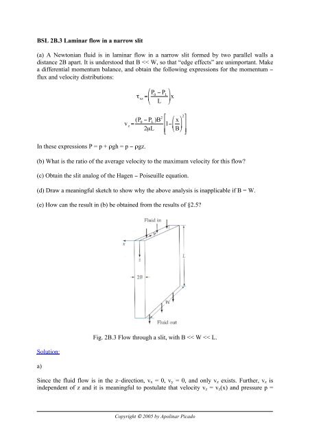
<strong>BSL</strong> 2B.3 Laminar flow in a narrow slit<br />
(a) A Newtonian fluid is in laminar flow in a narrow slit formed by two parallel walls a<br />
distance 2B apart. It is understood that B
€<br />
€<br />
€<br />
€<br />
€<br />
€<br />
€<br />
€<br />
p(z). The only nonvanishing components of the stress tensor are τxz = τzx, which depend only<br />
on x.<br />
Consider now a thin rectangular slab (shell) perpendicular to the x−direction extending a<br />
distance W in the y−direction and a distance L in the z−direction. A 'rate of z−momentum'<br />
balance over this thin shell of thickness Δx in the fluid is of the form:<br />
(LW) ( φxz − φ<br />
x<br />
xz<br />
x +Δx ) + (WΔx) ( φzz − φ<br />
z=0<br />
zz<br />
z= L)<br />
+ (ΔxLW)ρg = 0<br />
Dividing the above equation by LWΔx, and the limit taken as Δx approaches zero, we get<br />
∂φxz ∂x − φzz − φ<br />
z=0<br />
zz<br />
z= L − ρg = 0<br />
L<br />
At this point we have to write out explicitly what components φxz and φzz are, making use of<br />
the definition of φ in Eqs. 1.7-1 to 3 and the expressions for τxz and τzz in Table B.1. This<br />
ensures that we do not miss out any of the forms of momentum transport. Hence, we get<br />
φ xz = τ xz + ρv xv z = τ xz<br />
φ zz = p + τ zz + ρv zv z = p<br />
In accordance with the postulates that vz = vz(x), vx = 0, vy = 0, and p = p(z), we see that (i)<br />
since vx = 0, the term ρvxvz is zero; (ii) since vz = vz(x), the term τzz is zero; (iii) since vz =<br />
vz(x), the term ρvzvz is the same at both ends of the slit, so the convective terms are cancel<br />
out.<br />
dτxz dx − p0 − pL − ρg = 0<br />
L<br />
dτxz dx = p0 − pL + ρg<br />
L<br />
The right – hand side may be compactly and conveniently written by introducing the modified<br />
pressure P, which is the sum of the pressure and gravitational terms. The general definition of<br />
the modified pressure is P = p + ρgh, where h is the distance upward (in the direction opposed<br />
to gravity) from a reference plane of choice. Since the z−axis points downward in this<br />
problem, h = − z and therefore P = p − ρgz. Thus, P0 = p0 at z = 0 and PL = pL − ρgL at z = L<br />
giving p0 − pL + ρgL = P0 − PL.<br />
dx = P ⎛⎛<br />
0 − P ⎞⎞<br />
L<br />
⎜⎜ ⎟⎟<br />
⎝⎝ L ⎠⎠<br />
dτ xz<br />
Integration leads to the following expression for the shear stress distribution<br />
τxz = P0 − P ⎛⎛ ⎞⎞<br />
L<br />
⎜⎜ ⎟⎟ x + C1 ⎝⎝ L ⎠⎠<br />
€<br />
€<br />
Copyright © 2005 by Apolinar Picado
€<br />
€<br />
€<br />
€<br />
€<br />
€<br />
It is worth noting that the two last equations apply to Newtonian and non – Newtonian fluid.<br />
The constant of integration C1 is determined later using boundary conditions.<br />
Substituting Newton's law of viscosity for τxz in above equation gives<br />
−µ dv z<br />
dx = P0 − P ⎛⎛ ⎞⎞<br />
L<br />
⎜⎜ ⎟⎟ x + C1 ⎝⎝ L ⎠⎠<br />
The above first – order differential equation is simply integrated to obtain the following<br />
velocity profile<br />
v z = − P0 − P ⎛⎛ ⎞⎞<br />
L<br />
⎜⎜ ⎟⎟ x<br />
⎝⎝ 2µL ⎠⎠<br />
2 − C1 µ x + C2 Boundary conditions<br />
BC1: at x = B; vz = 0<br />
BC2: at x = − B; vz = 0<br />
Using these, the integration constants may be evaluated as C1 = 0 and C2 = (P0 – PL)B 2 /(2µL).<br />
Substituting C1 = 0 in the shear stress equation, the final expression is found to be linear as<br />
given by<br />
τxz = P0 − P ⎛⎛ ⎞⎞<br />
L<br />
⎜⎜ ⎟⎟ x<br />
⎝⎝ L ⎠⎠<br />
Further, substitution of the integration constants gives the final expression for the velocity<br />
profile as<br />
v z = (P 0 − P L )B 2<br />
2µL<br />
1− x<br />
⎡⎡ 2<br />
⎛⎛ ⎞⎞ ⎤⎤<br />
⎢⎢ ⎜⎜ ⎟⎟ ⎥⎥<br />
⎣⎣ ⎢⎢ ⎝⎝ B⎠⎠<br />
⎦⎦ ⎥⎥<br />
It is observed that the velocity distribution for laminar, incompressible flow of a Newtonian<br />
fluid in a plane narrow slit is parabolic.<br />
b)<br />
The maximum velocity occurs at x = 0 (where dvz/dx = 0). Therefore,<br />
v z,max = (P 0 − P L )B2<br />
2µL<br />
v z =v z,max 1− x ⎛⎛<br />
⎜⎜<br />
⎝⎝ B<br />
⎞⎞ ⎡⎡ 2⎤⎤<br />
⎢⎢ ⎟⎟ ⎥⎥<br />
⎣⎣ ⎢⎢ ⎠⎠ ⎦⎦ ⎥⎥<br />
Copyright © 2005 by Apolinar Picado
€<br />
€<br />
€<br />
€<br />
€<br />
€<br />
€<br />
The average velocity is obtained by dividing the volumetric flow rate by the cross – sectional<br />
area as shown below.<br />
v z =<br />
∫<br />
B<br />
∫<br />
∫<br />
W<br />
−B 0<br />
B<br />
−B<br />
v z = v z,max<br />
B<br />
v z = v z,max<br />
B<br />
v z<br />
v z,max<br />
= 2<br />
3<br />
∫<br />
v z(x)dydx<br />
∫<br />
0<br />
W<br />
⎛⎛<br />
dydx<br />
1− x2<br />
B 2<br />
B<br />
0 ⎜⎜<br />
⎝⎝<br />
2<br />
3 B<br />
⎛⎛ ⎞⎞<br />
⎜⎜ ⎟⎟<br />
⎝⎝ ⎠⎠<br />
⎞⎞<br />
⎟⎟ dx<br />
⎠⎠<br />
Thus, the ratio of the average velocity to the maximum velocity for Newtonian fluid flow in a<br />
narrow slit is 2/3.<br />
This seems reasonable since<br />
€<br />
v z /vz,max = ½ for flow in a circular pipe. For a slit a larger<br />
cross − sectional area carries fluid flowing at the larger velocity than for flow in a circular<br />
pipe. So v z /vz,max for slit > v z /vz,max for a circular pipe.<br />
c)<br />
€ The mass rate of flow € is the product of the density ρ, the cross − sectional area (2BW) and the<br />
average velocity v z .<br />
w = ρ (2BW) v z<br />
€<br />
w = ρ (2BW) 2 (P0 − PL )B<br />
3<br />
2<br />
2µL<br />
w = 2 (P0 − PL )B<br />
3<br />
3 Wρ<br />
µL<br />
The flow rate vs. pressure drop (w vs. ΔP) expression above is the slit analog of the Hagen –<br />
Poiseuille equation (originally for circular tubes). It is a result worth noting because it<br />
provides the starting point for creeping flow in many systems (e.g. radial flow between two<br />
parallel circular disks; and flow between two stationary concentric spheres).<br />
d)<br />
The above analysis is not applicable if B = W, because of the presence of a wall at y = 0 and y<br />
= B would cause vz to vary significantly in y in addition to x, then vz = vz (x, y).<br />
Copyright © 2005 by Apolinar Picado
€<br />
€<br />
€<br />
€<br />
If W = 2B, then a solution can be obtained for flow in a square duct.<br />
e)<br />
In Eq. 2.5-20, set both viscosities equal to µ, p0 − pL = P0 – PL, and set b equal to B.<br />
v z = (P 0 − P L )B2<br />
12µL<br />
⎛⎛ 8⎞⎞<br />
⎜⎜ ⎟⎟ =<br />
⎝⎝ 2⎠⎠<br />
(P0 − PL )B2<br />
3µL<br />
v z = 2<br />
2 ⋅ (P0 − PL )B2<br />
=<br />
3µL<br />
2 (P0 − PL )B<br />
3<br />
2<br />
2µL<br />
v z = 2<br />
3 v z,max<br />
v z<br />
v z,max<br />
= 2<br />
3<br />
Copyright © 2005 by Apolinar Picado


![[ ]x [ ]](https://img.yumpu.com/39572719/1/190x135/-x-.jpg?quality=85)