Precision & Performance: Floating Point and IEEE 754 Compliance ...
Precision & Performance: Floating Point and IEEE 754 Compliance ...
Precision & Performance: Floating Point and IEEE 754 Compliance ...

You also want an ePaper? Increase the reach of your titles
YUMPU automatically turns print PDFs into web optimized ePapers that Google loves.
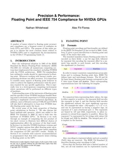
<strong>Precision</strong> & <strong>Performance</strong>:<br />
<strong>Floating</strong> <strong>Point</strong> <strong>and</strong> <strong>IEEE</strong> <strong>754</strong> <strong>Compliance</strong> for NVIDIA GPUs<br />
Nathan Whitehead Alex Fit-Florea<br />
ABSTRACT<br />
A number of issues related to floating point accuracy<br />
<strong>and</strong> compliance are a frequent source of confusion on<br />
both CPUs <strong>and</strong> GPUs. The purpose of this white paper<br />
is to discuss the most common issues related to<br />
NVIDIA GPUs <strong>and</strong> to supplement the documentation<br />
in the CUDA C Programming Guide [7].<br />
1. INTRODUCTION<br />
Since the widespread adoption in 1985 of the <strong>IEEE</strong><br />
St<strong>and</strong>ard for Binary <strong>Floating</strong>-<strong>Point</strong> Arithmetic (<strong>IEEE</strong><br />
<strong>754</strong>-1985 [1]) virtually all mainstream computing systems<br />
have implemented the st<strong>and</strong>ard, including NVIDIA<br />
with the CUDA architecture. <strong>IEEE</strong> <strong>754</strong> st<strong>and</strong>ardizes<br />
how arithmetic results should be approximated in floating<br />
point. Whenever working with inexact results, programming<br />
decisions can affect accuracy. It is important<br />
to consider many aspects of floating point behavior in<br />
order to achieve the highest performance with the precision<br />
required for any specific application. This is especially<br />
true in a heterogeneous computing environment<br />
where operations will be performed on different types<br />
of hardware.<br />
Underst<strong>and</strong>ing some of the intricacies of floating point<br />
<strong>and</strong> the specifics of how NVIDIA hardware h<strong>and</strong>les floating<br />
point is obviously important to CUDA programmers<br />
striving to implement correct numerical algorithms. In<br />
addition, users of libraries such as CUBLAS <strong>and</strong> CUFFT<br />
will also find it informative to learn how NVIDIA h<strong>and</strong>les<br />
floating point under the hood.<br />
We review some of the basic properties of floating<br />
point calculations in Section 2. We also discuss the<br />
fused multiply-add operator, which was added to the<br />
<strong>IEEE</strong> <strong>754</strong> st<strong>and</strong>ard in 2008 [2] <strong>and</strong> is built into the<br />
hardware of NVIDIA GPUs. In Section 3 we work<br />
through an example of computing the dot product of<br />
two short vectors to illustrate how different choices of<br />
implementation affect the accuracy of the final result.<br />
In Section 4 we describe NVIDIA hardware versions <strong>and</strong><br />
NVCC compiler options that affect floating point calculations.<br />
In Section 5 we consider some issues regarding<br />
the comparison of CPU <strong>and</strong> GPU results. Finally, in<br />
Section 6 we conclude with concrete recommendations<br />
to programmers that deal with numeric issues relating<br />
to floating point on the GPU.<br />
Permission to make digital or hard copies of all or part of this work<br />
for any use is granted without fee provided that copies bear this<br />
notice <strong>and</strong> the full citation on the first page.<br />
Copyright 2011 NVIDIA.<br />
2. FLOATING POINT<br />
2.1 Formats<br />
<strong>Floating</strong> point encodings <strong>and</strong> functionality are defined<br />
in the <strong>IEEE</strong> <strong>754</strong> St<strong>and</strong>ard [2] last revised in 2008. Goldberg<br />
[5] gives a good introduction to floating point <strong>and</strong><br />
many of the issues that arise.<br />
The st<strong>and</strong>ard m<strong>and</strong>ates binary floating point data be<br />
encoded on three fields: a one bit sign field, followed<br />
by exponent bits encoding the exponent offset by a numeric<br />
bias specific to each format, <strong>and</strong> bits encoding<br />
the signific<strong>and</strong> (or fraction).<br />
sign exponent fraction<br />
In order to ensure consistent computations across platforms<br />
<strong>and</strong> to exchange floating point data, <strong>IEEE</strong> <strong>754</strong><br />
defines basic <strong>and</strong> interchange formats. The 32 <strong>and</strong> 64<br />
bit basic binary floating point formats correspond to the<br />
C data types float <strong>and</strong> double. Their corresponding<br />
representations have the following bit lengths:<br />
float 1 8 23<br />
double 1 11 52<br />
For numerical data representing finite values, the sign<br />
is either negative or positive, the exponent field encodes<br />
the exponent in base 2, <strong>and</strong> the fraction field encodes<br />
the signific<strong>and</strong> without the most significant non-zero<br />
bit. For example the value −192 equals (−1) 1 ×2 7 ×1.5,<br />
<strong>and</strong> can be represented as having a negative sign, an<br />
exponent of 7, <strong>and</strong> a fractional part .5. The exponents<br />
are biased by 127 <strong>and</strong> 1023, respectively, to allow exponents<br />
to extend from negative to positive. Hence the<br />
exponent 7 is represented by bit strings with values 134<br />
for float <strong>and</strong> 1030 for double. The integral part of 1.<br />
is implicit in the fraction.<br />
float<br />
1 10000110 .100000000000000000000000<br />
double<br />
1 10000000110 .10000000000000000. . . 0000000<br />
Also, encodings to represent infinity <strong>and</strong> not-a-number<br />
(NaN) data are reserved. The <strong>IEEE</strong> <strong>754</strong> St<strong>and</strong>ard [2]<br />
describes floating point encodings in full.<br />
Given that the fraction field uses a limited number of<br />
bits, not all real numbers can be represented exactly.
For example the mathematical value of the fraction 2/3<br />
represented in binary is 0.10101010... which has an infinite<br />
number of bits after the binary point. The value<br />
2/3 must be rounded first in order to be represented<br />
as a floating point number with limited precision. The<br />
rules for rounding <strong>and</strong> the rounding modes are specified<br />
in <strong>IEEE</strong> <strong>754</strong>. The most frequently used is the<br />
round-to-nearest-or-even mode (abbreviated as roundto-nearest).<br />
The value 2/3 rounded in this mode is represented<br />
in binary as:<br />
float<br />
0 01111110 .01010101010101010101011<br />
double<br />
0 01111111110 .01010101010101010. . . 1010101<br />
The sign is positive <strong>and</strong> the stored exponent value<br />
represents an exponent of −1.<br />
2.2 Operations <strong>and</strong> Accuracy<br />
The <strong>IEEE</strong> <strong>754</strong> st<strong>and</strong>ard requires support for a h<strong>and</strong>ful<br />
of operations. These include the arithmetic operations<br />
add, subtract, multiply, divide, square root, fusedmultiply-add,<br />
remainder, conversion operations, scaling,<br />
sign operations, <strong>and</strong> comparisons. The results of<br />
these operations are guaranteed to be the same for all<br />
implementations of the st<strong>and</strong>ard, for a given format <strong>and</strong><br />
rounding mode.<br />
The rules <strong>and</strong> properties of mathematical arithmetic<br />
do not hold directly for floating point arithmetic because<br />
of floating point’s limited precision. For example,<br />
the table below shows single precision values A, B, <strong>and</strong><br />
C, <strong>and</strong> the mathematical exact value of their sum computed<br />
using different associativity.<br />
A = 2 1 × 1.00000000000000000000001<br />
B = 2 0 × 1.00000000000000000000001<br />
C = 2 3 × 1.00000000000000000000001<br />
(A + B) + C = 2 3 × 1.01100000000000000000001011<br />
A + (B + C) = 2 3 × 1.01100000000000000000001011<br />
Mathematically, (A + B) + C does equal A + (B + C).<br />
Let rn(x) denote one rounding step on x. Performing<br />
these same computations in single precision floating<br />
point arithmetic in round-to-nearest mode according to<br />
<strong>IEEE</strong> <strong>754</strong>, we obtain:<br />
A + B = 2 1 × 1.1000000000000000000000110000 . . .<br />
rn(A + B) = 2 1 × 1.10000000000000000000010<br />
B + C = 2 3 × 1.0010000000000000000000100100 . . .<br />
rn(B + C) = 2 3 × 1.00100000000000000000001<br />
A + B + C = 2 3 × 1.0110000000000000000000101100 . . .<br />
rn(rn(A + B) + C) = 2 3 × 1.01100000000000000000010<br />
rn(A + rn(B + C)) = 2 3 × 1.01100000000000000000001<br />
For reference, the exact, mathematical results are computed<br />
as well in the table above. Not only are the results<br />
computed according to <strong>IEEE</strong> <strong>754</strong> different from<br />
the exact mathematical results, but also the results corresponding<br />
to the sum rn(rn(A + B) + C) <strong>and</strong> the sum<br />
rn(A + rn(B + C)) are different from each other. In this<br />
case, rn(A + rn(B + C)) is closer to the correct mathematical<br />
result than rn(rn(A + B) + C).<br />
This example highlights that seemingly identical computations<br />
can produce different results even if all basic<br />
operations are computed in compliance with <strong>IEEE</strong> <strong>754</strong>.<br />
Here, the order in which operations are executed affects<br />
the accuracy of the result. The results are independent<br />
of the host system. These same results would be obtained<br />
using any microprocessor, CPU or GPU, which<br />
supports single precision floating point.<br />
2.3 The Fused Multiply-Add (FMA)<br />
In 2008 the <strong>IEEE</strong> <strong>754</strong> st<strong>and</strong>ard was revised to include<br />
the fused multiply-add operation (FMA). The FMA operation<br />
computes rn(X × Y + Z) with only one rounding<br />
step. Without the FMA operation the result would<br />
have to be computed as rn(rn(X × Y ) + Z) with two<br />
rounding steps, one for multiply <strong>and</strong> one for add. Because<br />
the FMA uses only a single rounding step the<br />
result is computed more accurately.<br />
Let’s consider an example to illustrate how the FMA<br />
operation works using decimal arithmetic first for clarity.<br />
Let’s compute x 2 − 1 in finite-precision with four<br />
digits of precision after the decimal point, or a total of<br />
five digits of precision including the leading digit before<br />
the decimal point.<br />
For x = 1.0008, the correct mathematical result is<br />
x 2 −1 = 1.60064×10 −4 . The closest number using only<br />
four digits after the decimal point is 1.6006 × 10 −4 . In<br />
this case rn(x 2 − 1) = 1.6006 × 10 −4 which corresponds<br />
to the fused multiply-add operation rn(x × x + (−1)).<br />
The alternative is to compute separate multiply <strong>and</strong> add<br />
steps. For the multiply, x 2 = 1.00160064, so rn(x 2 ) =<br />
1.0016. The final result is rn(rn(x 2 ) − 1) = 1.6000 ×<br />
10 −4 .<br />
Rounding the multiply <strong>and</strong> add separately yields a result<br />
that is wrong by 0.00064. The corresponding FMA<br />
computation is wrong by only 0.00004, <strong>and</strong> its result is<br />
closest to the correct mathematical answer. The results<br />
are summarized below:<br />
x = 1.0008<br />
x 2 = 1.00160064<br />
x 2 − 1 = 1.60064 × 10 −4 true value<br />
rn(x 2 − 1) = 1.6006 × 10 −4 fused multiply-add<br />
rn(x 2 ) = 1.0016 × 10 −4<br />
rn(rn(x 2 ) − 1) = 1.6000 × 10 −4 multiply, then add<br />
Below is another example, using binary single precision<br />
values:<br />
A = 2 0 × 1.00000000000000000000001<br />
B = −2 0 × 1.00000000000000000000010<br />
rn(A × A + B) = 2 −46 × 1.00000000000000000000000<br />
rn(rn(A × A) + B) = 0<br />
In this particular case, computing rn(rn(A × A) + B)<br />
as an <strong>IEEE</strong> <strong>754</strong> multiply followed by an <strong>IEEE</strong> <strong>754</strong> add<br />
loses all bits of precision, <strong>and</strong> the computed result is 0.<br />
The alternative of computing the FMA rn(A × A + B)<br />
provides a result equal to the mathematical value. In<br />
general, the fused-multiply-add operation generates more<br />
accurate results than computing one multiply followed<br />
by one add. The choice of whether or not to use the<br />
fused operation depends on whether the platform provides<br />
the operation <strong>and</strong> also on how the code is compiled.<br />
Figure 1 shows CUDA C code <strong>and</strong> output corresponding<br />
to inputs A <strong>and</strong> B <strong>and</strong> operations from the example<br />
above. The code is executed on two different hardware<br />
platforms: an x86-class CPU using SSE in single precision,<br />
<strong>and</strong> an NVIDIA GPU with compute capability
union {<br />
float f;<br />
unsigned int i;<br />
} a, b;<br />
float r;<br />
a.i = 0x3F800001;<br />
b.i = 0xBF800002;<br />
r = a.f * a.f + b.f;<br />
printf("a %.8g\n", a.f);<br />
printf("b %.8g\n", b.f);<br />
printf("r %.8g\n", r);<br />
x86-64 output:<br />
a: 1.0000001<br />
b: -1.0000002<br />
r: 0<br />
NVIDIA Fermi output:<br />
a: 1.0000001<br />
b: -1.0000002<br />
r: 1.4210855e-14<br />
Figure 1: Multiply <strong>and</strong> add code fragment <strong>and</strong><br />
output for x86 <strong>and</strong> NVIDIA Fermi GPU<br />
2.0. At the time this paper is written (Spring 2011)<br />
there are no commercially available x86 CPUs which<br />
offer hardware FMA. Because of this, the computed result<br />
in single precision in SSE would be 0. NVIDIA<br />
GPUs with compute capability 2.0 do offer hardware<br />
FMAs, so the result of executing this code will be the<br />
more accurate one by default. However, both results are<br />
correct according to the <strong>IEEE</strong> <strong>754</strong> st<strong>and</strong>ard. The code<br />
fragment was compiled without any special intrinsics or<br />
compiler options for either platform.<br />
The fused multiply-add helps avoid loss of precision<br />
during subtractive cancellation. Subtractive cancellation<br />
occurs during the addition of quantities of similar<br />
magnitude with opposite signs. In this case many of the<br />
leading bits cancel, leaving fewer meaningful bits of precision<br />
in the result. The fused multiply-add computes a<br />
double-width product during the multiplication. Thus<br />
even if subtractive cancellation occurs during the addition<br />
there are still enough valid bits remaining in the<br />
product to get a precise result with no loss of precision.<br />
3. DOT PRODUCT: AN ACCURACY EX-<br />
AMPLE<br />
Consider the problem of finding the dot product of<br />
two short vectors a <strong>and</strong> b both with four elements.<br />
⎡<br />
⎢<br />
a = ⎣<br />
a1<br />
a2<br />
a3<br />
a4<br />
⎤<br />
⎡<br />
⎥<br />
⎦ ⎢<br />
b = ⎣<br />
b1<br />
b2<br />
b3<br />
b4<br />
⎤<br />
⎥<br />
⎦ a · b = a1b1 + a2b2 + a3b3 + a4b4<br />
This operation is easy to write mathematically, but<br />
its implementation in software involves several choices.<br />
All of the strategies we will discuss use purely <strong>IEEE</strong> <strong>754</strong><br />
compliant operations.<br />
3.1 Example Algorithms<br />
We present three algorithms which differ in how the<br />
multiplications, additions, <strong>and</strong> possibly fused multiplyadds<br />
are organized. These algorithms are presented in<br />
Figures 2, 3, <strong>and</strong> 4. Each of the three algorithms is represented<br />
graphically. Individual operation are shown as<br />
a circle with arrows pointing from arguments to operations.<br />
The simplest way to compute the dot product is using<br />
a short loop as shown in Figure 2. The multiplications<br />
t = 0<br />
for i from 1 to 4<br />
p = rn(ai × bi)<br />
t = rn(t + p)<br />
return t<br />
Figure 2: The serial method uses a simple loop<br />
with separate multiplies <strong>and</strong> adds to compute<br />
the dot product of the vectors. The final result<br />
can be represented as ((((a1 ×b1)+(a2 ×b2))+(a3 ×<br />
b3)) + (a4 × b4)).<br />
t = 0<br />
for i from 1 to 4<br />
t = rn(ai × bi + t)<br />
return t<br />
Figure 3: The FMA method uses a simple loop<br />
with fused multiply-adds to compute the dot<br />
product of the vectors. The final result can be<br />
represented as a4 × b4 + (a3 × b3 + (a2 × b2 + (a1 ×<br />
b1 + 0))).<br />
<strong>and</strong> additions are done separately.<br />
A simple improvement to the algorithm is to use the<br />
fused multiply-add to do the multiply <strong>and</strong> addition in<br />
one step to improve accuracy. Figure 3 shows this version.<br />
Yet another way to compute the dot product is to use<br />
a divide-<strong>and</strong>-conquer strategy in which we first find the<br />
dot products of the first half <strong>and</strong> the second half of the<br />
vectors, then combine these results using addition. This<br />
is a recursive strategy; the base case is the dot product<br />
of vectors of length 1 which is a single multiply. Figure<br />
4 graphically illustrates this approach. We call this<br />
algorithm the parallel algorithm because the two subproblems<br />
can be computed in parallel as they have no<br />
dependencies. The algorithm does not require a parallel<br />
implementation, however; it can still be implemented<br />
with a single thread.<br />
3.2 Comparison<br />
All three algorithms for computing a dot product use<br />
<strong>IEEE</strong> <strong>754</strong> arithmetic <strong>and</strong> can be implemented on any<br />
system that supports the <strong>IEEE</strong> st<strong>and</strong>ard. In fact, an<br />
implementation of the serial algorithm on multiple systems<br />
will give exactly the same result. So will implementations<br />
of the FMA or parallel algorithms. How-
p1 = rn(a1 × b1)<br />
p2 = rn(a2 × b2)<br />
p3 = rn(a3 × b3)<br />
p4 = rn(a4 × b4)<br />
sleft = rn(p1 + p2)<br />
sright = rn(p3 + p4)<br />
t = rn(sleft + sright)<br />
return t<br />
Figure 4: The parallel method uses a tree to reduce<br />
all the products of individual elements into<br />
a final sum. The final result can be represented<br />
as ((a1 × b1) + (a2 × b2)) + ((a3 × b3) + (a4 × b4)).<br />
method result float value<br />
exact .0559587528435... 0x3D65350158...<br />
serial .0559588074 0x3D653510<br />
FMA .0559587515 0x3D653501<br />
parallel .0559587478 0x3D653500<br />
Figure 5: All three algorithms yield results<br />
slightly different from the correct mathematical<br />
dot product.<br />
ever, results computed by an implementation of the serial<br />
algorithm may differ from those computed by an<br />
implementation of the other two algorithms.<br />
For example, consider the vectors<br />
a = [1.907607, −.7862027, 1.147311, .9604002]<br />
b = [−.9355000, −.6915108, 1.724470, −.7097529]<br />
whose elements are r<strong>and</strong>omly chosen values between −1<br />
<strong>and</strong> 2. The accuracy of each algorithm corresponding<br />
to these inputs is shown in Figure 5.<br />
The main points to notice from the table are that<br />
each algorithm yields a different result, <strong>and</strong> they are<br />
all slightly different from the correct mathematical dot<br />
product. In this example the FMA version is the most<br />
accurate, <strong>and</strong> the parallel algorithm is more accurate<br />
than the serial algorithm. In our experience these results<br />
are typical; fused multiply-add significantly increases<br />
the accuracy of results, <strong>and</strong> parallel tree reductions<br />
for summation are usually much more accurate<br />
than serial summation.<br />
4. CUDA AND FLOATING POINT<br />
NVIDIA has extended the capabilities of GPUs with<br />
each successive hardware generation. Current generations<br />
of the NVIDIA architecture such as Tesla C2xxx,<br />
GTX 4xx, <strong>and</strong> GTX 5xx, support both single <strong>and</strong> double<br />
precision with <strong>IEEE</strong> <strong>754</strong> precision <strong>and</strong> include hardware<br />
support for fused multiply-add in both single <strong>and</strong><br />
double precision. Older NVIDIA architectures support<br />
some of these features but not others. In CUDA, the<br />
features supported by the GPU are encoded in the compute<br />
capability number. The runtime library supports<br />
a function call to determine the compute capability of<br />
a GPU at runtime; the CUDA C Programming Guide<br />
also includes a table of compute capabilities for many<br />
different devices [7].<br />
4.1 Compute capability 1.2 <strong>and</strong> below<br />
Devices with compute capability 1.2 <strong>and</strong> below support<br />
single precision only. In addition, not all operations<br />
in single precision on these GPUs are <strong>IEEE</strong> <strong>754</strong><br />
accurate. Denormal numbers (small numbers close to<br />
zero) are flushed to zero. Operations such as square<br />
root <strong>and</strong> division may not always result in the floating<br />
point value closest to the correct mathematical value.<br />
4.2 Compute capability 1.3<br />
Devices with compute capability 1.3 support both<br />
single <strong>and</strong> double precision floating point computation.<br />
Double precision operations are always <strong>IEEE</strong> <strong>754</strong> accurate.<br />
Single precision in devices of compute capability<br />
1.3 is unchanged from previous compute capabilities.<br />
In addition, the double precision hardware offers fused<br />
multiply-add. As described in Section 2.3, the fused<br />
multiply-add operation is faster <strong>and</strong> more accurate than<br />
separate multiplies <strong>and</strong> additions. There is no single<br />
precision fused multiply-add operation in compute capability<br />
1.3.<br />
4.3 Compute capability 2.0 <strong>and</strong> above<br />
Devices with compute capability 2.0 <strong>and</strong> above support<br />
both single <strong>and</strong> double precision <strong>IEEE</strong> <strong>754</strong> including<br />
fused multiply-add in both single <strong>and</strong> double precision.<br />
Operations such as square root <strong>and</strong> division will<br />
result in the floating point value closest to the correct<br />
mathematical result in both single <strong>and</strong> double precision,<br />
by default.<br />
4.4 Rounding modes<br />
The <strong>IEEE</strong> <strong>754</strong> st<strong>and</strong>ard defines four rounding modes:<br />
round-to-nearest, round towards positive, round towards<br />
negative, <strong>and</strong> round towards zero. CUDA supports<br />
all four modes. By default, operations use round-tonearest.<br />
Compiler intrinsics like the ones listed in the<br />
tables below can be used to select other rounding modes<br />
for individual operations.<br />
mode interpretation<br />
rn round to nearest, ties to even<br />
rz round towards zero<br />
ru round towards +∞<br />
rd round towards -∞
x + y addition<br />
__fadd_[rn|rz|ru|rd](x, y)<br />
x * y multiplication<br />
__fmul_[rn|rz|ru|rd](x, y)<br />
fmaf(x, y, z) FMA<br />
__fmaf_[rn|rz|ru|rd](x, y, z)<br />
1.0f / x reciprocal<br />
__frcp_[rn|rz|ru|rd](x)<br />
x / y division<br />
__fdiv_[rn|rz|ru|rd](x, y)<br />
sqrtf(x) square root<br />
__fsqrt_[rn|rz|ru|rd](x)<br />
x + y addition<br />
__dadd_[rn|rz|ru|rd](x, y)<br />
x * y multiplication<br />
__dmul_[rn|rz|ru|rd](x, y)<br />
fma(x, y, z) FMA<br />
__fma_[rn|rz|ru|rd](x, y, z)<br />
1.0 / x reciprocal<br />
__drcp_[rn|rz|ru|rd](x)<br />
x / y division<br />
__ddiv_[rn|rz|ru|rd](x, y)<br />
sqrt(x) square root<br />
__dsqrt_[rn|rz|ru|rd](x)<br />
4.5 Controlling fused multiply-add<br />
In general, the fused multiply-add operation is faster<br />
<strong>and</strong> more accurate than performing separate multiply<br />
<strong>and</strong> add operations. However, on occasion you may<br />
wish to disable the merging of multiplies <strong>and</strong> adds into<br />
fused multiply-add instructions. To inhibit this optimization<br />
one can write the multiplies <strong>and</strong> additions<br />
using intrinsics with explicit rounding mode as shown<br />
in the previous tables. Operations written directly as<br />
intrinsics are guaranteed to remain independent <strong>and</strong><br />
will not be merged into fused multiply-add instructions.<br />
With CUDA Fortran it is possible to disable FMA merging<br />
via a compiler flag.<br />
4.6 Compiler flags<br />
Compiler flags relevant to <strong>IEEE</strong> <strong>754</strong> operations are<br />
-ftz={true|false}, -prec-div={true|false}, <strong>and</strong><br />
-prec-sqrt={true|false}. These flags control single<br />
precision operations on devices of compute capability of<br />
2.0 or later.<br />
mode flags<br />
<strong>IEEE</strong> <strong>754</strong> mode<br />
(default)<br />
-ftz=false<br />
-prec-div=true<br />
-prec-sqrt=true<br />
fast mode -ftz=true<br />
-prec-div=false<br />
-prec-sqrt=false<br />
The default “<strong>IEEE</strong> <strong>754</strong> mode” means that single precision<br />
operations are correctly rounded <strong>and</strong> support denormals,<br />
as per the <strong>IEEE</strong> <strong>754</strong> st<strong>and</strong>ard. In the “fast<br />
mode” denormal numbers are flushed to zero, <strong>and</strong> the<br />
operations division <strong>and</strong> square root are not computed to<br />
the nearest floating point value. The flags have no effect<br />
on double precision or on devices of compute capability<br />
below 2.0.<br />
4.7 Differences from x86<br />
NVIDIA GPUs differ from the x86 architecture in<br />
that rounding modes are encoded within each floating<br />
point instruction instead of dynamically using a floating<br />
point control word. Trap h<strong>and</strong>lers for floating point exceptions<br />
are not supported. On the GPU there is no status<br />
flag to indicate when calculations have overflowed,<br />
underflowed, or have involved inexact arithmetic. Like<br />
SSE, the precision of each GPU operation is encoded<br />
in the instruction (for x87 the precision is controlled<br />
dynamically by the floating point control word).<br />
5. CONSIDERATIONS FOR A HETERO-<br />
GENEOUS WORLD<br />
5.1 Mathematical function accuracy<br />
So far we have only considered simple math operations<br />
such as addition, multiplication, division, <strong>and</strong><br />
square root. These operations are simple enough that<br />
computing the best floating point result (e.g. the closest<br />
in round-to-nearest) is reasonable. For other mathematical<br />
operations computing the best floating point<br />
result is harder.<br />
The problem is called the table maker’s dilemma. To<br />
guarantee the correctly rounded result, it is not generally<br />
enough to compute the function to a fixed high<br />
accuracy. There might still be rare cases where the error<br />
in the high accuracy result affects the rounding step<br />
at the lower accuracy.<br />
It is possible to solve the dilemma for particular functions<br />
by doing mathematical analysis <strong>and</strong> formal proofs [4],<br />
but most math libraries choose instead to give up the<br />
guarantee of correct rounding. Instead they provide implementations<br />
of math functions <strong>and</strong> document bounds<br />
on the relative error of the functions over the input<br />
range. For example, the double precision sin function<br />
in CUDA is guaranteed to be accurate to within 2 units<br />
in the last place (ulp) of the correctly rounded result. In<br />
other words, the difference between the computed result<br />
<strong>and</strong> the mathematical result is at most ±2 with respect<br />
to the least significant bit position of the fraction part<br />
of the floating point result.<br />
For most inputs the sin function produces the correctly<br />
rounded result. For some inputs the result is off<br />
by 1 ulp. For a small percentage of inputs the result is<br />
off by 2 ulp.<br />
Producing different results, even on the same system,<br />
is not uncommon when using a mix of precisions, libraries<br />
<strong>and</strong> hardware. Take for example the C code<br />
sequence shown in Figure 6. We compiled the code sequence<br />
on a 64-bit x86 platform using gcc version 4.4.3<br />
(Ubuntu 4.3.3-4ubuntu5).<br />
This shows that the result of computing cos(5992555.0)<br />
using a common library differs depending on whether<br />
the code is compiled in 32-bit mode or 64-bit mode.<br />
The consequence is that different math libraries cannot<br />
be expected to compute exactly the same result for a<br />
given input. This applies to GPU programming as well.<br />
Functions compiled for the GPU will use the NVIDIA<br />
CUDA math library implementation while functions compiled<br />
for the CPU will use the host compiler math library<br />
implementation (e.g. glibc on Linux). Because<br />
these implementations are independent <strong>and</strong> neither is
volatile float x = 5992555.0;<br />
printf("cos(%f): %.10g\n", x, cos(x));<br />
gcc test.c -lm -m64<br />
cos(5992555.000000): 3.320904615e-07<br />
gcc test.c -lm -m32<br />
cos(5992555.000000): 3.320904692e-07<br />
Figure 6: The computation of cosine using the<br />
glibc math library yields different results when<br />
compiled with -m32 <strong>and</strong> -m64.<br />
guaranteed to be correctly rounded, the results will often<br />
differ slightly.<br />
5.2 x87 <strong>and</strong> SSE<br />
One of the unfortunate realities of C compilers is that<br />
they are often poor at preserving <strong>IEEE</strong> <strong>754</strong> semantics<br />
of floating point operations [6]. This can be particularly<br />
confusing on platforms that support x87 <strong>and</strong> SSE operations.<br />
Just like CUDA operations, SSE operations are<br />
performed on single or double precision values, while<br />
x87 operations often use an additional internal 80-bit<br />
precision format. Sometimes the results of a computation<br />
using x87 can depend on whether an intermediate<br />
result was allocated to a register or stored to memory.<br />
Values stored to memory are rounded to the declared<br />
precision (e.g. single precision for float <strong>and</strong> double<br />
precision for double). Values kept in registers can remain<br />
in extended precision. Also, x87 instructions will<br />
often be used by default for 32-bit compiles but SSE<br />
instructions will be used by default for 64-bit compiles.<br />
Because of these issues, guaranteeing a specific precision<br />
level on the CPU can sometimes be tricky. When<br />
comparing CPU results to results computed on the GPU,<br />
it is generally best to compare using SSE instructions.<br />
SSE instructions follow <strong>IEEE</strong> <strong>754</strong> for single <strong>and</strong> double<br />
precision.<br />
On 32-bit x86 targets without SSE it can be helpful<br />
to declare variables using volatile <strong>and</strong> force floating<br />
point values to be stored to memory (/Op in Visual<br />
Studio <strong>and</strong> -ffloat-store in gcc). This moves results<br />
from extended precision registers into memory, where<br />
the precision is precisely single or double precision. Alternately,<br />
the x87 control word can be updated to set<br />
the precision to 24 or 53 bits using the assembly instruction<br />
fldcw or a compiler option such as -mpc32 or<br />
-mpc64 in gcc.<br />
5.3 Core Counts<br />
As we have shown in Section 3, the final values computed<br />
using <strong>IEEE</strong> <strong>754</strong> arithmetic can depend on implementation<br />
choices such as whether to use fused multiplyadd<br />
or whether additions are organized in series or parallel.<br />
These differences affect computation on the CPU<br />
<strong>and</strong> on the GPU.<br />
One example of the differences can arise from differences<br />
between the number of concurrent threads involved<br />
in a computation. On the GPU, a common design<br />
pattern is to have all threads in a block coordinate<br />
to do a parallel reduction on data within the block,<br />
followed by a serial reduction of the results from each<br />
block. Changing the number of threads per block reorganizes<br />
the reduction; if the reduction is addition, then<br />
the change rearranges parentheses in the long string of<br />
additions.<br />
Even if the same general strategy such as parallel<br />
reduction is used on the CPU <strong>and</strong> GPU, it is common<br />
to have widely different numbers of threads on the<br />
GPU compared to the CPU. For example, the GPU<br />
implementation might launch blocks with 128 threads<br />
per block, while the CPU implementation might use 4<br />
threads in total.<br />
5.4 Verifying GPU Results<br />
The same inputs will give the same results for individual<br />
<strong>IEEE</strong> <strong>754</strong> operations to a given precision on the<br />
CPU <strong>and</strong> GPU. As we have explained, there are many<br />
reasons why the same sequence of operations may not be<br />
performed on the CPU <strong>and</strong> GPU. The GPU has fused<br />
multiply-add while the CPU does not. Parallelizing algorithms<br />
may rearrange operations, yielding different<br />
numeric results. The CPU may be computing results in<br />
a precision higher than expected. Finally, many common<br />
mathematical functions are not required by the<br />
<strong>IEEE</strong> <strong>754</strong> st<strong>and</strong>ard to be correctly rounded so should<br />
not be expected to yield identical results between implementations.<br />
When porting numeric code from the CPU to the<br />
GPU of course it makes sense to use the x86 CPU results<br />
as a reference. But differences between the CPU<br />
result <strong>and</strong> GPU result must be interpreted carefully.<br />
Differences are not automatically evidence that the result<br />
computed by the GPU is wrong or that there is a<br />
problem on the GPU.<br />
Computing results in a high precision <strong>and</strong> then comparing<br />
to results computed in a lower precision can be<br />
helpful to see if the lower precision is adequate for a particular<br />
application. However, rounding high precision<br />
results to a lower precision is not equivalent to performing<br />
the entire computation in lower precision. This can<br />
sometimes be a problem when using x87 <strong>and</strong> comparing<br />
results against the GPU. The results of the CPU may<br />
be computed to an unexpectedly high extended precision<br />
for some or all of the operations. The GPU result<br />
will be computed using single or double precision only.<br />
6. CONCRETE RECOMMENDATIONS<br />
The key points we have covered are the following.<br />
Use the fused multiply-add operator.<br />
The fused multiply-add operator on the GPU has<br />
high performance <strong>and</strong> increases the accuracy of computations.<br />
No special flags or function calls are needed<br />
to gain this benefit in CUDA programs. Underst<strong>and</strong><br />
that a hardware fused multiply-add operation is not yet<br />
available on the CPU, which can cause differences in numerical<br />
results.<br />
Compare results carefully.<br />
Even in the strict world of <strong>IEEE</strong> <strong>754</strong> operations, minor<br />
details such as organization of parentheses or thread<br />
counts can affect the final result. Take this into account<br />
when doing comparisons between implementations.
Know the capabilities of your GPU.<br />
The numerical capabilities are encoded in the compute<br />
capability number of your GPU. Devices of compute<br />
capability 2.0 <strong>and</strong> later are capable of single <strong>and</strong><br />
double precision arithmetic following the <strong>IEEE</strong> <strong>754</strong> st<strong>and</strong>ard,<br />
<strong>and</strong> have hardware units for performing fused<br />
multiply-add in both single <strong>and</strong> double precision.<br />
Take advantage of the CUDA math library functions.<br />
These functions are documented in Appendix C of the<br />
CUDA C Programming Guide [7]. The math library<br />
includes all the math functions listed in the C99 st<strong>and</strong>ard<br />
[3] plus some additional useful functions. These<br />
functions have been tuned for a reasonable compromise<br />
between performance <strong>and</strong> accuracy.<br />
We constantly strive to improve the quality of our<br />
math library functionality. Please let us know about<br />
any functions that you require that we do not provide,<br />
or if the accuracy or performance of any of our functions<br />
does not meet your needs. Leave comments in the<br />
NVIDIA CUDA forum 1 or join the Registered Developer<br />
Program 2 <strong>and</strong> file a bug with your feedback.<br />
7. ACKNOWLEDGEMENTS<br />
Thanks to Ujval Kapasi, Kurt Wall, Paul Sidenblad,<br />
Massimiliano Fatica, Everett Phillips, Norbert Juffa,<br />
<strong>and</strong> Will Ramey for their helpful comments <strong>and</strong> suggestions.<br />
1 http://forums.nvidia.com/index.php?showforum=62<br />
2 http://developer.nvidia.com/<br />
join-nvidia-registered-developer-program<br />
8. REFERENCES<br />
[1] ANSI/<strong>IEEE</strong> <strong>754</strong>-1985. American National<br />
St<strong>and</strong>ard — <strong>IEEE</strong> St<strong>and</strong>ard for Binary<br />
<strong>Floating</strong>-<strong>Point</strong> Arithmetic. American National<br />
St<strong>and</strong>ards Institute, Inc., New York, 1985.<br />
[2] <strong>IEEE</strong> <strong>754</strong>-2008. <strong>IEEE</strong> <strong>754</strong>–2008 St<strong>and</strong>ard for<br />
<strong>Floating</strong>-<strong>Point</strong> Arithmetic. August 2008.<br />
[3] ISO/IEC 9899:1999(E). Programming<br />
languages—C. American National St<strong>and</strong>ards<br />
Institute, Inc., New York, 1999.<br />
[4] Catherine Daramy-Loirat, David Defour, Florent<br />
de Dinechin, Matthieu Gallet, Nicolas Gast, <strong>and</strong><br />
Jean-Michel Muller. CR-LIBM: A library of<br />
correctly rounded elementary functions in<br />
double-precision, February 2005.<br />
[5] David Goldberg. What every computer scientist<br />
should know about floating-point arithmetic. ACM<br />
Computing Surveys, March 1991. Edited reprint<br />
available at: http://download.oracle.com/docs/<br />
cd/E19957-01/806-3568/ncg_goldberg.html.<br />
[6] David Monniaux. The pitfalls of verifying<br />
floating-point computations. ACM Transactions on<br />
Programming Languages <strong>and</strong> Systems, May 2008.<br />
[7] NVIDIA. CUDA C Programming Guide Version<br />
4.0, 2011.