20th Century operation of the Tromsø Ionosonde - IPS - Radio and ...
20th Century operation of the Tromsø Ionosonde - IPS - Radio and ...
20th Century operation of the Tromsø Ionosonde - IPS - Radio and ...

You also want an ePaper? Increase the reach of your titles
YUMPU automatically turns print PDFs into web optimized ePapers that Google loves.
20 th <strong>Century</strong> <strong>operation</strong> <strong>of</strong> <strong>the</strong> <strong>Tromsø</strong> <strong>Ionosonde</strong><br />
C. M. Hall <strong>and</strong> T. L. Hansen<br />
<strong>Tromsø</strong> Geophysical Observatory, University <strong>of</strong> <strong>Tromsø</strong>, Norway<br />
Reproduced from Advances in Polar Upper Atmosphere Research,<br />
No. 17(2003) p. 155-166<br />
Abstract. A history <strong>of</strong> ionospheric soundings from <strong>Tromsø</strong> <strong>and</strong> its vicinity in<br />
nor<strong>the</strong>rn Norway (69°N, 19°E) between 1932 <strong>and</strong> 1999 is given.<br />
Introduction<br />
The recent reviews by Rishbeth [2001] <strong>and</strong> Schröder [2002] tell us something <strong>of</strong> <strong>the</strong><br />
history <strong>of</strong> solar-terrestrial physics. The successful transatlantic radio transmissions<br />
performed by Marconi in 1901 lead Kennelly <strong>and</strong> Heaviside to hypo<strong>the</strong>size <strong>the</strong><br />
existence <strong>of</strong> some reflecting layer in <strong>the</strong> atmosphere. Experiments in <strong>the</strong> 1920s by<br />
Appleton <strong>and</strong> Barnett [1926] <strong>and</strong> Breit <strong>and</strong> Tuve [1926] confirmed this. The Second<br />
International Polar Year was to be in 1932-3 <strong>and</strong> <strong>the</strong> <strong>Tromsø</strong> Auroral Observatory<br />
stood complete in <strong>the</strong> summer <strong>of</strong> 1929. Under <strong>the</strong> URSI umbrella, Sir George<br />
Simpson proposed ionospheric measurements in Nor<strong>the</strong>rn Norway <strong>and</strong> was <strong>the</strong>refore<br />
invited to <strong>Tromsø</strong> by Lars Vegard, <strong>the</strong> <strong>the</strong>n President <strong>of</strong> <strong>the</strong> Norwegian Institute <strong>of</strong><br />
Cosmic Physics. Thus surprisingly few years elapsed between <strong>the</strong>se first experiments<br />
<strong>and</strong> Sir Edward Appleton’s arrival in <strong>Tromsø</strong> (69°N, 19°E), in 1932 in order to<br />
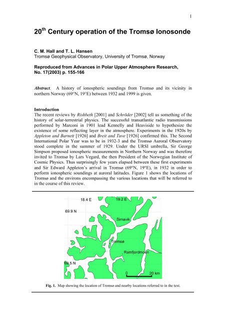
perform ionospheric soundings at auroral latitudes. Figure 1 shows <strong>the</strong> locations <strong>of</strong><br />
<strong>Tromsø</strong> <strong>and</strong> <strong>the</strong> environs encompassing <strong>the</strong> various locations that will be referred to<br />
in <strong>the</strong> course <strong>of</strong> this review.<br />
Fig. 1. Map showing <strong>the</strong> location <strong>of</strong> <strong>Tromsø</strong> <strong>and</strong> nearby locations referred to in <strong>the</strong> text.<br />
1
These first ionospheric soundings were intended to establish <strong>and</strong> map <strong>the</strong> little<br />
understood Kenelly-Heaviside layer (later to be <strong>the</strong> E-layer toge<strong>the</strong>r with <strong>the</strong><br />
Appleton- or F-layer). The practical use <strong>of</strong> such information was clear: <strong>the</strong> importance<br />
<strong>of</strong> radio communications prior to <strong>the</strong> period <strong>of</strong> increasing unrest in Europe at that time<br />
could not be understated. During WWII transatlantic communication became a vital<br />
tool <strong>and</strong> this carried on through <strong>the</strong> subsequent cold-war years. Today, with satellite<br />
communications <strong>and</strong> high b<strong>and</strong>widths commonplace, monitoring <strong>the</strong> ionosphere is<br />
becoming gradually less important. In <strong>the</strong> 1920s, climatic change was a concept that<br />
received little attention; in <strong>the</strong> 21 st century, however, it is even on <strong>the</strong> curricula <strong>of</strong><br />
many junior schools. Who in Slough <strong>and</strong> <strong>Tromsø</strong> in 1924 could have foreseen <strong>the</strong><br />
application <strong>of</strong> ionospheric sounding to climatic research? Rishbeth <strong>and</strong> Clilverd<br />
[1999] provide a most accessible insight, with Rishbeth <strong>and</strong> Roble [1992] <strong>and</strong> Roble<br />
<strong>and</strong> Dickinson [1989] giving more depth.<br />
Many time-series <strong>of</strong> ionospheric data exist. One notable example is that from <strong>the</strong><br />
Sodankylä instrument in nor<strong>the</strong>rn Finl<strong>and</strong> <strong>and</strong> described by Ulich <strong>and</strong> Turunen<br />
[1997]. The Sodankylä dataset is very special because <strong>the</strong> analysis (“scaling” in<br />
ionosonde parlance) has been performed by <strong>the</strong> same person throughout, <strong>and</strong> <strong>the</strong>refore<br />
susceptibility to systematic error is ra<strong>the</strong>r less than if a succession <strong>of</strong> employees had<br />
performed <strong>the</strong> work during <strong>the</strong> almost half a century <strong>of</strong> <strong>operation</strong>. In contrast,<br />
although ionospheric soundings at <strong>Tromsø</strong> currently span almost 70 years, many<br />
different persons have performed <strong>the</strong> scaling. Not only that, but both <strong>the</strong> instrument<br />
<strong>and</strong> its precise location have changed during that course <strong>of</strong> time. Historical<br />
information about <strong>the</strong> instrument must be taken into account when analysing time<br />
series because abrupt systematic changes in derived ionospheric parameters due to<br />
subjectivity <strong>of</strong> <strong>the</strong> scaling <strong>operation</strong>, calibration <strong>of</strong> <strong>the</strong> instrument etc., may easily be<br />
interpreted incorrectly as a trend. Exploratory trend analyses <strong>of</strong> <strong>Tromsø</strong> data have<br />
recently been performed by Hall <strong>and</strong> Cannon [2001, 2002] following a feasibility<br />
study Hall [2001a]. These studies, however illustrated <strong>the</strong> need to document <strong>the</strong><br />
history <strong>of</strong> <strong>the</strong> <strong>Tromsø</strong> ionosonde; much information is still in living memory, but will<br />
not always remain so. This sad fact is <strong>the</strong> inevitable consequence <strong>of</strong> time-series<br />
durations exceeding not only <strong>the</strong> careers <strong>of</strong> scientists but also <strong>the</strong>ir lifetimes.<br />
We shall divide <strong>the</strong> history into three sections for ease <strong>of</strong> accessibility: (i) <strong>the</strong> early<br />
years, from Appleton’s expedition in 1932 until <strong>the</strong> true start <strong>of</strong> comprehensive<br />
ionogram analysis in 1951, (ii) <strong>the</strong> stable “middle”years, 1951 to 1980, <strong>and</strong> (iii) <strong>the</strong><br />
later years, 1980 to present, somewhat characterised by technological, administrative<br />
<strong>and</strong> funding changes. Table 1 summarises <strong>the</strong> various events in chronological order.<br />
1932-1950: Appleton <strong>and</strong> <strong>the</strong> war years<br />
The very first <strong>operation</strong>s at Simavik near <strong>Tromsø</strong> (see Figure 1) are described in no<br />
little detail by Appleton et al. [1937]. Simavik, some 17 km almost due N <strong>of</strong> <strong>Tromsø</strong><br />
was selected for <strong>the</strong> transmitter location due to power supply considerations; this<br />
seems remarkable today since although <strong>the</strong> transmitter was initially operated at 3kW,<br />
subsequent <strong>operation</strong> for <strong>the</strong> Polar Year was only 100W. The receiver, on <strong>the</strong> o<strong>the</strong>r<br />
h<strong>and</strong> was located at <strong>Tromsø</strong>. Table 2a gives <strong>the</strong> salient features <strong>of</strong> <strong>the</strong> sounder;<br />
o<strong>the</strong>rwise, <strong>the</strong> instrument is described exhaustively by Appleton et al. [1937]. It<br />
appears that assembly was performed in less than a week! (between 15 th <strong>and</strong> 22 nd<br />
July). Ra<strong>the</strong>r than <strong>the</strong> more familiar continuous observing programme used today,<br />
specific dates were allocated specific types <strong>of</strong> measurement. Each <strong>of</strong> <strong>the</strong> four<br />
measurement types was performed on one occasion each month between August 1932<br />
2
<strong>and</strong> August 1933. Observations concentrated on critical frequencies almost<br />
exclusively: variation <strong>of</strong> E- <strong>and</strong> F-region critical frequencies with local time was<br />
studied <strong>and</strong> many comparisons were made with geomagnetic observations. Total<br />
absorption appears to be a feature Appleton et al. [1937] found considerably<br />
interesting since it was not a common occurrence at Slough.<br />
The success <strong>of</strong> <strong>the</strong> 1932-33 observations clearly impressed <strong>the</strong> leadership <strong>of</strong> <strong>the</strong><br />
Auroral Observatory <strong>and</strong> help was obtained to construct a copy <strong>of</strong> <strong>the</strong> Slough<br />
instrument, this being <strong>of</strong> a slightly different design to <strong>the</strong> Simavik instrument, again<br />
detailed by Appleton et al. [1937] (Table 2b). Funding was provided by <strong>the</strong><br />
Norwegian Scientific Research Fund (literal translation) <strong>and</strong> <strong>the</strong> Norwegian<br />
Broadcasting Company, totalling 11,000 Norwegian Crowns (around €1400). This<br />
new, Norwegian instrument came on <strong>the</strong> air in April 1935, <strong>and</strong> this time both<br />
transmitter <strong>and</strong> receiver were located at <strong>the</strong> Auroral Observatory. Harang [1937]<br />
describes <strong>the</strong> instrument <strong>and</strong> <strong>the</strong> operating method, <strong>and</strong> goes on to provide details <strong>of</strong><br />
<strong>the</strong> results. Again, only critical frequencies were recorded, although by now thrice<br />
daily <strong>and</strong> including some comments regarding <strong>the</strong> appearance <strong>of</strong> <strong>the</strong> echo. Figure 2<br />
shows <strong>the</strong> transmitter unit as it looked in 1936. Figure 3 shows some <strong>of</strong> <strong>the</strong> early<br />
results from May 1935 along with <strong>the</strong> interpretations [from Harang, 1937].<br />
Fig. 2. The first Norwegian ionosonde transmitter, copied from <strong>the</strong> Slough instrument, from 1936<br />
[Larsen <strong>and</strong> Berger, 2000].<br />
The instrument remained in <strong>operation</strong> throughout <strong>the</strong> war years; however, a German<br />
instrument was also in <strong>operation</strong> only a few hundred metres from <strong>the</strong> Auroral<br />
Observatory during WWII. This ionosonde was acquired by <strong>the</strong> Norwegians<br />
eventually <strong>and</strong> <strong>the</strong> delta-antennae re-located <strong>and</strong> used toge<strong>the</strong>r with <strong>the</strong> original<br />
Norwegian instrument from 1946 onwards. After <strong>the</strong> war, <strong>the</strong> British National<br />
Physical Laboratory (NPL) produced a better ionosonde <strong>and</strong> one <strong>of</strong> <strong>the</strong>se was<br />
purchased by <strong>the</strong> Norwegian Defence Research Establishment (NDRE) in Kjeller near<br />
3
Oslo at <strong>the</strong> end <strong>of</strong> 1949. Eventually, a similar system was installed in <strong>Tromsø</strong>, finally<br />
replacing <strong>the</strong> original in Autumn 1950 after almost 16 years <strong>of</strong> service.<br />
1951-1980: The cold war<br />
The arrival <strong>of</strong> <strong>the</strong> NPL ionosonde (Table 2c <strong>and</strong> Figure 4) heralded a more organised<br />
publication <strong>of</strong> results, <strong>and</strong>, importantly a fuller scaling <strong>of</strong> each ionogram.<br />
Fig. 3. Early results from <strong>the</strong> first Norwegian ionosonde on a variety <strong>of</strong> days between May 1935 <strong>and</strong><br />
October 1936. The line drawings show <strong>the</strong> operators’ interpretations <strong>of</strong> <strong>the</strong> echoes, <strong>and</strong>, importantly <strong>the</strong><br />
calibrations necessary for any re-analysis <strong>of</strong> <strong>the</strong> archived photographic recordings [Harang, 1937]<br />
Heights were read <strong>of</strong>f <strong>the</strong> ionograms <strong>and</strong> <strong>the</strong> transmission parameter M(3000)F2<br />
determined. Fur<strong>the</strong>rmore, soundings were taken more <strong>of</strong>ten, <strong>and</strong> monthly summaries<br />
4
<strong>of</strong> median values were published. There is evidence that antenna improvements were<br />
made in 1956, presumably for <strong>the</strong> International Geophysical Year (IGY 1957); sadly,<br />
<strong>the</strong>se are undocumented, except for <strong>the</strong> existence <strong>of</strong> a somewhat uninformative<br />
photograph (not reproduced here)..<br />
A disadvantage with <strong>the</strong> NPL ionosonde was that it took around 5 min to obtain a full<br />
sounding. In <strong>the</strong> 1960s a Swedish company, “Magnetic AB”, began manufacturing<br />
faster <strong>and</strong> more automated instruments; one <strong>of</strong> <strong>the</strong>se was purchased (Table 2d <strong>and</strong><br />
Figure 5) <strong>and</strong> replaced <strong>the</strong> NPL unit in <strong>the</strong> spring <strong>of</strong> 1968. Despite considerable<br />
dem<strong>and</strong>s for maintenance, <strong>the</strong> improved quality <strong>of</strong> ionograms was considered to give<br />
such improved final results that <strong>the</strong> effort was worthwhile. While <strong>the</strong> preceding<br />
ionosondes had made recordings onto photographic paper, <strong>the</strong> Magnetic AB device<br />
recorded to 35mm film, each ionogram occupying 72mm; <strong>the</strong> earliest such film in <strong>the</strong><br />
Auroral Observatory archives being dated 3 rd November 1969.<br />
Fig 4. The NPL ionosonde [Larsen <strong>and</strong> Berger, 2000].<br />
Meanwhile, a field station at nearby Ramfjordmoen (see Figure 1) was built with a<br />
view to housing both a new MF radar [Hall 2001b] <strong>and</strong> ionosonde. A new 60m mast<br />
was obtained for <strong>the</strong> purpose, but <strong>the</strong> Magnetic AB ionosonde’s fate was for it to<br />
remain at <strong>the</strong> Auroral Observatory where it st<strong>and</strong>s today. Instead, recognising <strong>the</strong><br />
advances in technology since <strong>the</strong> development <strong>of</strong> <strong>the</strong> Magnetic AB instrument, <strong>the</strong><br />
Auroral Observatory staff decided to build an ionosonde <strong>the</strong>mselves. This new<br />
5
instrument was taken into <strong>operation</strong> in January 1980 at Ramfjordmoen <strong>and</strong> <strong>the</strong><br />
Magnetic AB instrument discontinued on 27 th December 1979.<br />
Fig. 5. The “Magnetic AB” ionosonde receiver <strong>and</strong> recorder. (Photo: Chris Hall)<br />
1980-2000: The newer technologies<br />
Due to <strong>the</strong> presence <strong>of</strong> <strong>the</strong> MF radar at <strong>and</strong> <strong>the</strong> plans for establishing an incoherent<br />
scatter radar nearby (i.e. <strong>the</strong> European Incoherent Scatter facility, “EISCAT”) <strong>the</strong><br />
Ramfjordmoen site presented a scientifically attractive location for an ionosonde.<br />
With <strong>the</strong> large log-periodic antenna hanging from <strong>the</strong> 60m mast, higher power, <strong>and</strong><br />
sophistications such as Barker <strong>and</strong> complementary coded pulses made this a<br />
considerably more powerful <strong>and</strong> flexible instrument than <strong>the</strong> predecessors (Figure 6,<br />
Table 2e) [von Zahn <strong>and</strong> Hansen, 1988].<br />
6
Fig. 6. The Auroral Observatory ionosonde [Larsen <strong>and</strong> Berger, 2000].<br />
Initially recording was done to film with each ionogram lying transversely across<br />
18mm <strong>of</strong> a 35mm film. Eventually film recording was phased out in favour <strong>of</strong><br />
exclusive recording to magnetic tape. Today, film records exist until <strong>the</strong> end <strong>of</strong> 1984,<br />
<strong>and</strong> approximately half <strong>of</strong> <strong>the</strong>se have been scanned into digital form at <strong>the</strong> time <strong>of</strong><br />
writing. The magnetic tape records have been extracted to o<strong>the</strong>r formats for safe<br />
archiving. The Auroral observatory ionosonde proved an invaluable addition to<br />
calibration <strong>of</strong> <strong>the</strong> newly established EISCAT radar <strong>and</strong> not least as a diagnostic for<br />
geophysical conditions during EISCAT observations. The publications resulting from<br />
EISCAT <strong>and</strong> MF-radar studies in which ionosonde data was involved to some degree<br />
are numerous <strong>and</strong> no attempt will be made to compile an exhaustive list here. Due to<br />
lack <strong>of</strong> interest in long-term routine activities, however, regular scaling <strong>of</strong> <strong>the</strong><br />
ionograms fell by <strong>the</strong> wayside during this period. The reports giving daily scaling<br />
parameters <strong>and</strong> monthly means/medians have been sorely missed since 1980.<br />
Moreover, due to <strong>the</strong> large number <strong>of</strong> soundings performed (typically one every 15<br />
minutes) <strong>the</strong> task <strong>of</strong> scaling <strong>the</strong> data a posteriori is virtually insurmountable. Steps are<br />
being taken to scale ionograms from local midday only, as an ongoing project.<br />
In 1992, <strong>the</strong> British Defence Research Agency (“DRA”), later <strong>the</strong> Defence Evaluation<br />
<strong>and</strong> Research Agency (“DERA”) <strong>and</strong> currently QinetiQ provided a University <strong>of</strong><br />
Massachusetts Lowell DPS-4 [Reinisch et al., 1992] sounder which was connected to<br />
<strong>the</strong> simultaneously improved antenna in place <strong>of</strong> <strong>the</strong> Auroral Observatory instrument.<br />
The Lowell instrument has <strong>the</strong> capability <strong>of</strong> real-time scaling <strong>of</strong> ionograms using <strong>the</strong><br />
ARTIST-4 system. While still requiring a degree <strong>of</strong> manual validation (ARTIST-4 is<br />
not felt to be 100% reliable by everyone!) <strong>the</strong> task <strong>of</strong> producing regular reports <strong>of</strong><br />
ionospheric sounding parameters is no longer insuperable. The Web-based<br />
information given by <strong>the</strong> above URLs is supplemented by Table 2f. Figure 7 shows<br />
<strong>the</strong> current sounder, while Figure 8 shows <strong>the</strong> antenna with <strong>the</strong> rhombic transmitter<br />
elements that <strong>the</strong> constituted <strong>the</strong> upgrade in 1992. Reception is on loop antennae.<br />
7
Fig. 7. The Lowell ionosonde. The Lowell unit itself is beneath <strong>the</strong> computer monitor. The rack to <strong>the</strong><br />
left contains frequency reference equipment including synchronisation with nearby instruments.<br />
(Photo: Bjørnar Hansen)<br />
8
Fig. 8. The current transmitter antenna arrangement at Ramfjordmoen. (Photo: Chris Hall)<br />
Summary<br />
We have seen that only a decade after <strong>the</strong> first ionospheric soundings, measurements<br />
were already being made in <strong>the</strong> auroral zone at <strong>Tromsø</strong> (69°). Thus <strong>the</strong> establishment<br />
<strong>of</strong> regular soundings at such a remote location in <strong>the</strong> mid 30’s was quite noteworthy.<br />
The war years <strong>and</strong> subsequent cold-war prompted considerable development <strong>of</strong><br />
ionosondes, but at <strong>the</strong> same time events caused somewhat interrupted <strong>operation</strong>, at<br />
least until 1950 <strong>and</strong> changing configuration <strong>of</strong> <strong>the</strong> instrument. In later years, after<br />
1980, changes in political <strong>and</strong> economical climates <strong>and</strong>, not least, in scientific<br />
philosophy again introduced changes in ionosonde <strong>operation</strong>. While, prior to 1980,<br />
9
funding had favoured manpower dem<strong>and</strong>ing work (instrument maintenance <strong>and</strong><br />
manual analysis <strong>and</strong> report-writing), more expensive hardware investments<br />
characterised <strong>the</strong> last two decades <strong>of</strong> <strong>the</strong> millennium, <strong>the</strong> “exciting” new equipment<br />
leading to reductions in personnel involvement in <strong>the</strong> more “boring” tasks <strong>of</strong><br />
maintaining <strong>the</strong> long-term observation sequences. Although modern computing<br />
techniques <strong>and</strong> signal processing concepts such as neural networks have enabled<br />
automatic ionogram scaling, <strong>the</strong> results are not so reliable that manual quality control<br />
is superfluous. This means that at <strong>the</strong> time <strong>of</strong> writing <strong>the</strong> automatic scaling <strong>of</strong><br />
ionograms by <strong>the</strong> Lowell instrument still requires manual checking before <strong>the</strong> data<br />
may be used for scientific purposes, <strong>and</strong> funding to perform this task is scarcely<br />
available.<br />
Despite <strong>the</strong>se difficulties, <strong>the</strong> <strong>Tromsø</strong> dataset represents one <strong>of</strong> <strong>the</strong> longest, if not <strong>the</strong><br />
longest at such high latitude. Efforts are being made to st<strong>and</strong>ardise <strong>the</strong> dataset such<br />
that time series <strong>of</strong> selected parameters will be available to <strong>the</strong> scientific community<br />
for <strong>the</strong> entire period 1932 to present with minimal interruption. In order to evaluate<br />
<strong>the</strong> resulting dataset, documentation <strong>of</strong> <strong>the</strong> instrument’s history will be necessary in<br />
order that changes in instrumentation <strong>and</strong> analysis procedures will not be<br />
misinterpreted as effects <strong>of</strong> <strong>the</strong> solar-terrestrial system.<br />
Acknowledgements. The authors are indebted to Reidulv Larsen. Luis F. Alberca has<br />
supplemented our information on <strong>the</strong> Magnetic AB instrument. National Physical<br />
Laboratory (NPL) has supplied information on <strong>the</strong>ir instrument. Thanks also go to<br />
Bill Wright <strong>and</strong> Henry Rishbeth. The authors thank <strong>the</strong> National Institute <strong>of</strong> Polar<br />
Research, Tokyo, for persmission to reproduce this manuscript.<br />
References<br />
Appleton, E.V., The investigation <strong>and</strong> forecasting <strong>of</strong> ionospheric conditions, IEE, 94,<br />
186-199, 1947.<br />
Appleton, E.V. <strong>and</strong> M.A.F. Barnett, On wireless interference phenomena between<br />
ground waves <strong>and</strong> waves deviated by <strong>the</strong> upper atmosphere, Proc. Roy. Soc. A, 113,<br />
450-458, 1926<br />
Appleton, E.V., R. Naismith <strong>and</strong> L.J. Ingram, British radio observations during <strong>the</strong><br />
second International Polar Year 1932-33, Phil. Trans. A, 236, 191-259, 1937.<br />
Breit <strong>and</strong> Tuve, A test <strong>of</strong> <strong>the</strong> existence <strong>of</strong> <strong>the</strong> conducting layer, Phys. Rev., 28, 554-<br />
575, 1926<br />
Hall, C.M. <strong>and</strong> P.S. Cannon, Indication <strong>of</strong> <strong>the</strong> shrinking atmosphere above <strong>Tromsø</strong><br />
(69°N 19°E), Atmos, Phys. Lett., in press 2001.<br />
Hall, C.M., Climatic mesospheric cooling: Employing <strong>the</strong> long time-series <strong>of</strong><br />
ionospheric soundings from Norwegian stations, Mem. Nat. Inst. Polar Res., Spec.<br />
Issue, 54, 21-28, 2001a.<br />
Hall, C.M., The Ramfjormoen MF radar (69°N, 19°E): Application development<br />
1990-2000, J. Atmos. Solar-Terr. Phys., 63, 171-179, 2001b.<br />
10
Hall, C.M. <strong>and</strong> P.S. Cannon, Trends in foF2 above <strong>Tromsø</strong> (69°N 19°E), Geophys.<br />
Res. Lett., 29(3), 2128, doi:10.1029/2002GL016259, 2002.<br />
Harang, L., Results <strong>of</strong> radio echo observations for <strong>the</strong> years 1935 <strong>and</strong> 1936, Det<br />
Norske Institutt for Kosmisk Fysikk, 11, 24pp, John Greig, Bergen, Norway, 1937.<br />
Larsen, R., <strong>and</strong> S. Berger, Nordlysobservatoriet – historie og erindringer, University<br />
<strong>of</strong> <strong>Tromsø</strong>, Norway, in Norwegian, 71pp, 2000.<br />
Reinisch, B.W., D.M. Haines. <strong>and</strong> W.S. Kuklinski, "The New Portable Digisonde for<br />
Vertical <strong>and</strong> Oblique Sounding," AGARD-CP-502, 1992.<br />
Rishbeth, H., The centenary <strong>of</strong> solar-terrestrial physics, J. Atmos. Solar-Terr. Phys,<br />
63, 1883-1890, 2001.<br />
Rishbeth, H. <strong>and</strong> M. Clilverd, Long-term change in <strong>the</strong> upper atmosphere, Astronomy<br />
<strong>and</strong> Geophysics, 40, 3.26-3.28, 1999.<br />
Rishbeth, H. <strong>and</strong> R.G. Roble, Cooling <strong>of</strong> <strong>the</strong> upper atmosphere by enhanced<br />
greenhouse gases - modelling <strong>of</strong> <strong>the</strong>rmospheric <strong>and</strong> ionospheric effects, Planet.<br />
Space Sci., 40, 1011-1026, 1992.<br />
Roble, R.G. <strong>and</strong> R.E. Dickinson, How will changes in carbon-dioxide <strong>and</strong> methane<br />
modify <strong>the</strong> mean structure <strong>of</strong> <strong>the</strong> mesosphere <strong>and</strong> <strong>the</strong>rmosphere? Geophys. Res.<br />
Lett., 16, 1441-1444, 1989.<br />
Rosén, G., The Swedish manufactured ionosphere recorder, Elektronik, 7, 32-38,<br />
1967.<br />
Schröder, W., Comment on <strong>the</strong> paper “The centenary <strong>of</strong> solar-terrestrial physics”, J.<br />
Atmos. Solar-Terr. Phys, 64, 1675-1677, 2002<br />
Ulich, Th. <strong>and</strong> E. Turunen, Evidence for long-term cooling <strong>of</strong> <strong>the</strong> upper atmosphere.<br />
Geophys. Res. Lett., 24, 1103-1106, 1997.<br />
von Zahn, U., <strong>and</strong> T.L. Hansen, Sudden neutral sodium layers: a strong link to<br />
sporadic E layers, J. Atmos. Terr. Phys., 50, 93-104, 1988.<br />
11
Table 1.<br />
year(s) Event Reference<br />
1932-33 Instrument similar to that at Slough installed: transmitter at<br />
Simavik, receiver at <strong>Tromsø</strong><br />
Appleton et al., 1937<br />
1935 Copy <strong>of</strong> Slough instrument installed at Auroral Observatory Appleton et al., 1937<br />
1946 Antennae replaced with delta antennae<br />
1950 NPL Mk II ionosonde installed at Auroral Observatory<br />
1956<br />
Larsen <strong>and</strong> Berger, 2000<br />
Appleton, 1947<br />
Antenna improvements undocumented<br />
1968 Magnetic AB unit replaced NPL unit<br />
1980 Magnetic AB unit (at Auroral Observatory) superceded by<br />
Auroral Observatory unit at Ramfjordmoen<br />
1992 Lowell ionosonde replaced <strong>the</strong> Auroral Observatory unit<br />
(collaboration between Univ. <strong>Tromsø</strong> <strong>and</strong> QinetiQ)<br />
Rosén, 1967<br />
von Zahn <strong>and</strong> Hansen,<br />
1988<br />
Reinisch et al., 1992<br />
12
Table 2. Instruments overview<br />
(a) (b) (c) (d) (e) (f)<br />
Polar Year instrument<br />
(1932-1933)<br />
location Transmitter at Simavik,<br />
69.8° N, 19.0°E <strong>and</strong><br />
receiver at <strong>Tromsø</strong>,<br />
69.7° N, 18.9°E<br />
antenna type thought to be crossed<br />
dipoles 30km apart<br />
Copy <strong>of</strong> Slough<br />
instrument<br />
(1935-1950)<br />
<strong>Tromsø</strong>,<br />
69.7° N, 18.9°E<br />
crossed dipoles<br />
(same location);<br />
delta from 1946<br />
pulse repetition<br />
frequency<br />
pulse type single, 100 µs duration single, 100 µs<br />
duration<br />
NPL Mk II<br />
instrument<br />
(1950-1968)<br />
<strong>Tromsø</strong>,<br />
69.7° N, 18.9°E<br />
Magnetic AB “J5W”<br />
instrument<br />
(1968-1979)<br />
<strong>Tromsø</strong>,<br />
69.7° N, 18.9°E<br />
delta delta [Larsen <strong>and</strong><br />
Berger, 2000]<br />
Auroral Observatory<br />
instrument<br />
(1980-1992)<br />
Ramfjordmoen,<br />
69.6° N, 19.2°E<br />
Lowell instrument<br />
(1992-present)<br />
Ramfjordmoen,<br />
69.6° N, 19.2°E<br />
inverted log-periodic rhombic<br />
50 Hz 50 Hz 50 Hz 50 Hz N/A (asynchronous) 200 Hz<br />
single, presumably<br />
100 µs duration<br />
single,70-100 µs<br />
duration<br />
2 x 8 bit<br />
complementary code<br />
with 20µs elements<br />
13<br />
2 x 16 bit<br />
complementary code<br />
with 17µs elements<br />
peak power(normal<br />
<strong>operation</strong>)<br />
100 W not known 1-1.5 kW 35 kW 2kW 300 W<br />
range resolution 30 km not known better than 5% height marks every 6 km 5 km<br />
(calibration in 1955) 20 km, accurate to<br />
5%<br />
frequency coverage 0.6-10.0 MHz 1-12 MHz 0.7-24.6 MHz 0.25-20 MHz 1 -16 MHz<br />
Typically 1-12.0<br />
programmable MHz, but<br />
programmable<br />
frequency resolution 250 kHz 2 cm photographic marks at every 100 marks at every 1 240 frequencies 50 kHz<br />
paper / MHz kHz<br />
MHz, accurate to linearly or<br />
5%<br />
logarithmically<br />
distributed<br />
sweep time (typical<br />
frequency range)<br />
determined by operator 1 min 5 min 1 min 2-3 min 5-6 min