Download pdf

SIO 210: Global water masses and overturning
Lynne Talley Fall, 2012
Dec. 12 3-6 PM Final exam.
Mostly CLOSED BOOK EXAM – 1 page of notes allowed, front and
back, handwritten or typed. Calculators recommended.
Tutorials: after class today. Next Monday and Tuesday, time TBA
• Summary of circulation
• Summary of water masses
– Primary layers (4) for each ocean and sources
– T/S
• Meridional overturning
• Global overturning
• Role of air/sea fluxes and diffusivity
• Reading: parts of DPO Chapter 14

Upper ocean circulation
Gyres, western boundary currents, Antarctic Circumpolar Current,
equatorial circulations Schmitz (1995) (DPO Fig. 14.1)

Absolute surface height, related to
surface geostrophic velocity
Maximenko et al., GRL, 2003 (DPO Fig. 14.2)

200 and 1000 dbar circulation rel. to 2000 dbar
Shrinkage of
strong part of
ST gyres to
west and pole
(into the
WBC)
Roemmich and
Gilson, 2009
DPO Fig. 14.3

Surface circulation (absolute steric height from
hydrography)
Similar to Maximenko et al on previous slide
(Reid, 1994, 1997, 2003)

Circulation at 2000 dbar (adjusted steric height) (Reid, 1994, 1997,
2003)
2000 dbar
Greatly reduced subtropical gyres, continued ACC and equatorial
zonal flows, weak circulations elsewhere.
DPO Fig. 14.4a

Circulation at 4000 dbar (adjusted steric height)
4000 dbar
Below depth of NADW in S. Atlantic
Dominated by topography. Deep Western Boundary Currents, deep
cyclonic flows in some isolated basins
(Reid, 1994, 1997, 2003) DPO Fig. 14.4b

Global meridional overturning circulation
• Because sources of densest waters are in the northern N. Atlantic/
Nordic Seas (NADW) and in the Antarctic (AABW), interesting to see
how these fill the global ocean, upwell and return in upper ocean back to
source regions"
• Common to look at NET MERIDIONAL TRANSPORT across latitudes.
Most useful to look at this in isopycnal layers (not depth layers), since
flow is mostly along isopycnals."
• Also look at heat transport and freshwater transport this way."
• Choice of isopycnal layers is related to water masses. We can see
signature of meridional overturn by looking at the intermediate, deep and
abyssal water masses."
• Therefore, FIRST return here to global water mass description and the
go back to meridional overturn"

Calculation of meridional overturn
Use a zonal, coast-to-coast, top-to-bottom section
Compute geostrophic velocities, and estimate Ekman
transport
Calculate zonally-integrated transports in layers (isopycnal
layers or pressure layers)
Total transport through section should equal any leakages
(such as about 1 Sv for Bering Strait)

Calculation of meridional overturning
DPO Fig. 14.5

Net meridional transports in isopycnal
layers

Calculation of meridional overturn
Example: 24°N and 36°N N. Atlantic
(Roemmich and Wunsch, JGR 1985)
Location Temp. section
Smoothed
geostrophic
velocities
Meridional
transports

Meridional Overturning Streamfunction
Example of an Atlantic overturning streamfunction (from a
circulation model). Numbers are transport in Sverdrups. From
Gent (2000).

Meridional Overturning Streamfunction
Global zonal average: Results from P-OMIP at GFDL in Princeton
(2003)
http://www.frontier.iarc.uaf.edu/pomip/results.php

Meridional Overturning Streamfunction
GLOBAL Lumpkin and Speer (2007)

Meridional Overturning Streamfunction
Atlantic and Indian-Pacific Lumpkin and Speer (2007)

Global mass transport
(Ganachaud and Wunsch, 2000)

Schematics of the overturn: based on water mass
concepts and quantitative estimates of overturning
transport
Broecker “conveyor belt”
Simplification of NADW global overturning circulation ALONE
Missing: AABW global overturning circulation, actual ocean
connectivities
Broecker (1981) (DPO Fig. 14.10)

Global overturning schematic
More complete view based on major water mass transformations and
quantitative overturning transports
DPO Fig. 14.11a

Global overturning with Southern Ocean
perspective
After
Schmitz
(1995)
DPO Fig.
14.11b

Global overturning in zonally-averaged
view
DPO Fig. 14.11c

Heat transported by ocean circulation (big arrows)
Air-sea heat flux: Red shading - ocean gains heat. Blue -
ocean loses heat.

Global heat transport
(Ganachaud and Wunsch, 2000)

Global heat transport
(Ganachaud and Wunsch, 2000)

Water mass review: 4 layer view of the global
ocean
(1) Upper layer: ventilated thermocline. Includes Mode Waters,
Central Water, subtropical Underwater (salinity maximum
water)
(2) Intermediate layer: Labrador Sea Water, Mediterranean
Overflow Water, Red Sea Water, North Pacific Intermediate
Water, Antarctic Intermediate Water
(3) Deep layer: North Atlantic Deep Water, Pacific Deep Water
(also known as Common Water), Indian Deep Water,
Circumpolar Deep Water
(4) Bottom layer: Antarctic Bottom Water (aka Lower
Circumpolar Deep Water)
Remember these layer numbers!

(1) Upper ocean water masses
Central Waters (main subtropical thermocline, derived
from broad subduction of subtropical surface waters)
(not illustrated here)
• Subtropical Underwater (ST gyre, shallow salinity
maxima, derived from subduction of saltiest ST surface
water) (not illustrated here)
• Mode Waters (upper ocean, thick layers) (figure)
Hanawa and Talley (2001)

(2) Intermediate water summary
Low salinity: Labrador Sea
Water, North Pacific
Intermediate Water, Antarctic
Intermediate Water
High salinity: Mediterranean
Water, Red Sea Water
Talley (2008)

(3, 4) Deep water partial summary
(3) Nordic Seas Overflow
waters, contributing to
NADW
(4) Antarctic Bottom Water in
Weddell, Ross Seas and
Adelie Coast
Talley (1997)

Fraction of NADW vs. AABW
At about 2500-3000 m At the bottom
Johnson (2008) in DPO Figs. S14.4 and S14.5 (partially in fig. 14.15)

(1)
(3)
(4)
(2)

(2)
(3)
Oxygen in the Atlantic at 25W
(1)
(4)
(1) Upper
(2) AAIW
and LSW
(3) NADW
(4) AABW

Salinity in the Pacific (150°W)
(2)
(3)
(1)
(4)
(1) Upper
(2) AAIW
and
NPIW
(3) PDW
(4) LCBW
(AABW)

Oxygen in mid-Pacific (150W)
(2)
(4)
(1)
(3)
(1) Upper
(2) AAIW
and
NPIW
(3) PDW
(4) LCBW
(AABW)

Silicate in mid-Pacific (150W)
(2)
(1)
(4)
(3)
(1) Upper
(2) AAIW
and
NPIW
(3) PDW
(4) LCBW
(AABW)

delC14 in mid-Pacific (150W)
(2)
(1)
(4)
(3)
Very negative -
oldest water

Eastern Indian water masses
(4)
(2)
(3)
(1)
(3)
(2)
(1) Upper
(2) AAIW
and
RSW
(3) NADW
and IDW
(4) LCBW
(AABW)

Eastern Indian water masses: oxygen
(4)
(2)
(1)
(3)

Global deep water potential temperaturesalinity
0°C
Pacific
Deep Water
4°C
Antarctic
Bottom Water
Indian Deep
Water
Worthington, 1982
North Atlantic
Deep Water

Extra slides: diffusive balance

What about the upwelling
part of the meridional
overturn?
Profiles of potential temperature and
salinity from the central Pacific
showing nearly uniform abyssal
values and nearly exponential profile
up to about 1000 m."
Model with upwelling velocity and
vertical diffusion."
Obtain global values of "
w = 1.2 cm/day"
This gives an upwelling transport of
about 8 Sv for the Pacific"
Obtain diffusivity of"
κ = 1.3 cm 2 sec -1 = 1 x 10 -4 m 2 sec -1 "
Munk (1966)"

What about the upwelling part of the meridional
overturn?
Diffusion (diapycnal, i.e. across isopycnals) is required to return
convected/cooled waters back upwards to surface (better to
balance cooling effect from upward rising deep water)
It can be argued that the diapycnal diffusivity governs the overall
strength of the overturn, rather than the convection rates (which
are small).
The loop must close (Sandstrom theorem)

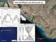
What causes the
diapycnal diffusivity?
They argue it is both tides
(surface tides creating internal
tides, creating internal waves
that break in the deep ocean
and cause turbulence)
And wind
(creating internal waves that
break in the deep ocean, or
eddies)
Munk and Wunsch (1998)

Relation of tides and wind to diapycnal diffusivity
From Jayne et al (Oceanography, 2004)

Relation of tides to diapycnal diffusivity
From Jayne et al (Oceanography, 2004)