Computing for accelerator physics Ilya Agapov, 7/12/09, DESY ...
Computing for accelerator physics Ilya Agapov, 7/12/09, DESY ...
Computing for accelerator physics Ilya Agapov, 7/12/09, DESY ...

You also want an ePaper? Increase the reach of your titles
YUMPU automatically turns print PDFs into web optimized ePapers that Google loves.
<strong>Computing</strong> <strong>for</strong> <strong>accelerator</strong> <strong>physics</strong><br />
<strong>Ilya</strong> <strong>Agapov</strong>, 7/<strong>12</strong>/<strong>09</strong>, <strong>DESY</strong> <strong>Computing</strong> Seminar
Contents<br />
Overview of <strong>accelerator</strong>s and computing requirements<br />
Electromagnetic field and thermal calculations<br />
Accelerator optics and beam dynamics codes<br />
Collective effects<br />
Energy deposition calculations and machinedetector interface<br />
Start to end <strong>accelerator</strong> simulations<br />
Control systems, online <strong>accelerator</strong> modeling and diagnostics
Areas where computing plays a role<br />
I will cover beam <strong>physics</strong><br />
and some controls issues
Basic <strong>accelerator</strong> types and components<br />
Linear Accelerators (injectors, linear collider,<br />
FEL, spallation neutron sources)<br />
Cyclotrons<br />
Synchrotrons (light sources, storage rings)<br />
Advanced <strong>accelerator</strong> concepts (plasmawakefield)
Linear <strong>accelerator</strong>s<br />
Injectorts <strong>for</strong> synchrotrons<br />
Neutron sources<br />
Linear colliders (SLC, ILC, CLIC)<br />
Acceleratordriven nuclear power<br />
Ion therapy<br />
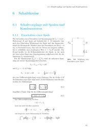
<strong>DESY</strong> XFEL Layout<br />
100keV test injector at PSI Accelerating cavity (from ACCEL) Dipole (from APS Argonne)
Synchrotrons<br />
HEP and nuclear <strong>physics</strong><br />
Circular colliders<br />
Light sources
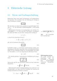
Plasmawakefield acceleration<br />
Use wakes created in plasma by intense electron or laser beams<br />
Accelerating tp ~1GeV over ~ 3 cm (would take ~1030m with RF)<br />
Challenges: energy spread, beam emittance,<br />
maintaining accelerating gradient, module staging<br />
Proof of concept SLAC, LBNL<br />
From CERN Courier June 2007
<strong>Computing</strong> in the project lifecycle
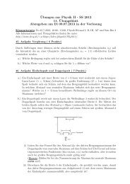
EM field calculations<br />
LHC main quad, ROXIE (from Russenschuk) Cavity electric field from www.gdfidl.de
Heat transfer, mechanical stress<br />
Stress and heat transfer calculations <strong>for</strong> dumps, targets, cryostats<br />
ANSYS<br />
AUTODYN (now part of ANSYS)
CST particle studio<br />
Collimator wakefiels (www.cst.com) Particle gun
vectorfields.com<br />
OPERA2D, OPERA3D<br />
Magnetostatics, thermal, quench,...<br />
Commercial codes<br />
Pros: CADlevel graphics, powerful mesh generation and solvers<br />
Contras: expensive, hard to extend
Wakefield code ECHO (TU Darmstadt / <strong>DESY</strong>)<br />
moving mesh<br />
bunch<br />
Slides S<br />
I. Zagorodnov <strong>DESY</strong>)<br />
Electromagnetic<br />
Code <strong>for</strong><br />
Handling<br />
Of<br />
Harmful<br />
Collective<br />
Effects<br />
Zagorodnov I, Weiland T., TE/TM Field Solver <strong>for</strong> Particle Beam Simulations without<br />
Numerical Cherenkov Radiation// Physical Review – STAB,8, 2005.<br />
Zagorodnov I., Indirect Methods <strong>for</strong> Wake Potential Integration // Physical Review<br />
STAB, 9, 2006.
in 2.5D stand alone application<br />
in 3D only solver, modelling and meshing in CST Microwave Studio<br />
Model and<br />
mesh in CST<br />
Microwave<br />
Studio<br />
Wakefield code ECHO (TU Darmstadt / <strong>DESY</strong>)<br />
Preprocessor<br />
in Matlab<br />
ECHO 3D<br />
Solver<br />
It allows <strong>for</strong> accurate calculations on conventional PC with<br />
only 1 p rocessor. To be p aralleliz ed …<br />
Postprocessor<br />
in Matlab
Beam optics<br />
Accelerator dimensions given by:<br />
maximum accelerating E field (linear)<br />
maximum bending magnet strength (circular)<br />
Tasks of beam optics –<br />
steer the beam to the experimental station meeting the constraints:<br />
✔ geometrical layout steering with dipole magnets – e.g. Desy to Schenefeld<br />
✔ fit in the aperture (focusing)<br />
✔ provide necessary beam sizes at experimental stations (focusing)<br />
✔ correct chromatic effects (focusing depending on energy)<br />
✔ in circular <strong>accelerator</strong>s – in addition provide stability<br />
Common approach (strong focusing) – build <strong>accelerator</strong>s from blocks similar to light optics e.g.<br />
dipole magnet – bend, quadrupole – focus/defocus, sextupole correct aberrations,<br />
RF cavity accelerate
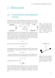
Linear optics<br />
Start with equations of singleparticle motion in the EM fields<br />
In a coordinate system going with a reference onaxis particle all building blocks can be<br />
represented by parametrized coordinate trans<strong>for</strong>mations<br />
where x,x', y, y' – particle coordinates and trajectory angles with respect to reference orbit<br />
Each trans<strong>for</strong>m depends on few parameters (usually just one).<br />
For basic optics linear approximation is sufficient. The trans<strong>for</strong>m is a matrix<br />
Taken from A. Streun,<br />
lectures at ETH
Linear optics<br />
A typical parametrization – through socalled twiss parameters<br />
A beam transport system (e.g. beam parameters) easily given by matrix multiplication.<br />
Writing a program to SIMULATE linear beam optics is straight<strong>for</strong>ward and can be<br />
done in a matter of days (<strong>for</strong>tran) or hours (matlab, mathematica, python, root etc.).<br />
Almost every computerinclined <strong>accelerator</strong> specialist has probably done it.<br />
Computeraided design:<br />
Too many free parameters. Still designed by humans from analytical principles<br />
starting from simple building blocks (FODO cell; final doublet/triplet)<br />
Only tuning (matching) of optics: find exact magnet settings to fit the beam size at IP<br />
Further issues, e.g.:<br />
Powering constraints<br />
xs= s cos s<br />
Cost issues (tunnel length minimization, required current minimization)<br />
Attempts at multiobjective genetic optimization have been made
Complications<br />
Some magnet types can be more complicated (e.g. LHC magnet with spool pieces;<br />
fringes etc.)<br />
Sextupoles and higher order multipoles should be included (compute chromatic<br />
functions)<br />
Collective effects – at least simple calculations useful (Intrabeam scattering)<br />
Aperture and layout in<strong>for</strong>mation (to go to a more engineering design)<br />
Input <strong>for</strong>mats (portability between codes still bad but improving)<br />
tracking required <strong>for</strong>:<br />
Steering algorithms <strong>for</strong> linacs (PLACET)<br />
For strongly nonlinear fields (extraction through a quad pocket) no sensible<br />
parametrization exists<br />
Longtern stability in storage rings – small perturbations play role – symplectic<br />
integrators (nonlinear dynamics)<br />
Presence of synchrotron radiation, gas scattering
Steering (PLACET code, D.Schulte, A.Latina et al.)<br />
Slides by A.Latina (FNAL)
Longterm stability, dynamic aperture<br />
Poincare section <strong>for</strong> linear (left) and nonlinear maps (right)<br />
Determining stability <strong>for</strong> largeamplitude particles requires longterm tracking<br />
Symplectic integrators to avoid large error accumulation<br />
Long term stability under influence of small random perturbations (RF noise, scattering)<br />
requires sofisticated computeintensive techniques (e.g. 6D FokkerPlanck equation)<br />
Spin dynamics in storage rings<br />
Codes: COSY, PTC,…<br />
Julia Set
MADX<br />
Widely used beam optics code www.cern.ch/mad<br />
LHC standard; has builtin high precision integrators (PTC), treats hight order multipoles<br />
Comprehensive set of beam <strong>physics</strong> processes<br />
Matching of beam parameters<br />
Spits out optics tables, can be plotted with external tools or builtin ps driver<br />
call file="../LHC-cell.seq";<br />
kqf = 0.01<strong>09</strong>88503297557 ;<br />
kqd = -0.011623337240602 ;<br />
Beam, particle = proton, sequence=lhccell, energy = 450.0,<br />
NPART=1.05E11, sige= 4.5e-4 ;<br />
use,period=lhccell;<br />
select, flag=twiss, clear;<br />
select, flag=twiss,column=s,name,betx,bety,mux,muy;<br />
twiss, sequence=lhccell,file='twiss-output';<br />
match,sequence=lhccell;<br />
constraint,sequence=lhccell,range=#e,mux=0.28,muy=0.31;<br />
vary,name=kqf,step=1.0e-6;<br />
vary,name=kqd,step=1.0e-6;<br />
lmdif,calls=500,tolerance=1.e-21;<br />
endmatch;<br />
value, kqf;<br />
value, kqd;
Collective effects<br />
a computational <strong>physics</strong> research area similar to plasma simulations<br />
Wakes and space charge (gdfidl, echo)<br />
Wakefield acceleration (PIC OSIRIS)<br />
Beambeam effects in colliders (GUINEAPIG)<br />
Electron clouds (codes: HEADTAIL, ECLOUD, FAKTOR2)
Energy deposition and machinedetector<br />
interface<br />
Was not a problem in the early years<br />
With more beam energy/intensity and superconducting magnets particle losses<br />
due to scattering, collimation system per<strong>for</strong>mance etc. become more critical<br />
Similar type of calculations as with HEP detectors (showers), but need to link it<br />
with beam dynamics in the machine<br />
Interfacing MonteCarlo radiation transport (FLUKA, GEANT4, MCNP, MARS) to<br />
<strong>accelerator</strong> tracking<br />
Examples: STRUCT/MARS at FNAL; FLUKA/SIXTRACK <strong>for</strong> LHC; BDSIM<br />
(standalone GEANT4 based tracking <strong>for</strong> ILC and ATF2)
BDSIM<br />
Complicated geometries are possible (e.g. extraction with electron and photon<br />
dump lines, bottom left).<br />
Detailed or simplified equipment models (e.g. laserwires)<br />
Tracking in vacuum + secondaries<br />
All Geant4 <strong>physics</strong> + fast tracking in vacuum and variance reduction techniques<br />
Energy deposition<br />
based on Geant4 + Root<br />
Detector interface – Mokka and xml<br />
29
Energy deposition, collimation, halo and backgrounds at ILC<br />
ILC collimation system (top left), electron and photon halo (top right)<br />
power losses in the extraction line (bottom left), energy deposition in a<br />
final focus quadrupole (bottom right)<br />
30
Start to end simulations<br />
Several codes staged to simulate the whole <strong>accelerator</strong>, typically from injector to<br />
the experimental station<br />
IMPACTT (Photoinjector), ELEGANT (Accelerator), Genesis (FEL process) <strong>for</strong> LCLS<br />
(Y Ding et al.)<br />
ASTRA + ELEGANT <strong>for</strong> PSI injector test facility (Y. KIM et al.)<br />
ASTRA + ELEGANT + + CSRTRACK + GENESIS <strong>for</strong> <strong>DESY</strong> XFEL<br />
MERLINbased <strong>for</strong> ILC (D. Krucker et al.)<br />
PLACET + BDSIM <strong>for</strong> CLIC (codes run in parallel, PLACET compute the wakefields<br />
and BDSIM tracks the secondaries and computes energy deposition)
Control Systems and online optics analysis<br />
Control system to drive individual hardware & processes<br />
Process examples:<br />
Ramp, injection, extraction, orbit correction<br />
Advanced concepts:<br />
GAN (Global Accelerator Network)<br />
LHC@FNAL remote operation centre <strong>for</strong> CMS and machine https://lhcatfnal.fnal.gov/<br />
Online models and flight simulators – virtual <strong>accelerator</strong> to plug control software<br />
✔ optics server at PSI’s SLS, CORBAbased, <strong>for</strong> orbit correction<br />
✔ ATF2 flight simulator<br />
✔ LHC online model
For complex machines the control system should be modelbased<br />
33
LHC Online model<br />
Provide virtual <strong>accelerator</strong> <strong>for</strong> software testing<br />
Virtual <strong>accelerator</strong> <strong>for</strong> safety checks during beam steering<br />
Online optics matching to help with beam steering<br />
Online optics error fitting<br />
Very detailed aperture and machine imperfection database<br />
Model corrections depending on operation conditions<br />
Clientserver architecture, javabased gui and control system interface, pythonbased<br />
server with MADX as the primary computation engine<br />
Ad hoc python scripting<br />
Used <strong>for</strong> LHC commissioning
Operator console – virtual mode<br />
35
User interface <strong>for</strong> interactive expert mode <br />
fully exploiting the <strong>accelerator</strong> model<br />
36
Example: injection and dump commissioning<br />
Full aperture model <strong>for</strong> injected and circulating (including septum alignment)<br />
OM used <strong>for</strong> orbit steering to detect aperture bottlenecks (oscillating bumps)<br />
Check that the beam is steering onto a collimator when kicker off<br />
Aperture bottleneck detected based on BLM data, confirmed by radiation<br />
survey and cured by realignment<br />
Magnetic error fitting from orbit and dispersion measurements<br />
37
Aperture measurements (arcs)<br />
Free oscillations with different starting phases generated by OM<br />
Closed bumps <strong>for</strong> bottlenecks<br />
Looking at BLM readings<br />
38
CMS beam crossing (from CERN logbook 03 Dec 20<strong>09</strong>)<br />
39
General data management issues<br />
Data rates/storage requirements less than HEP (even multiturn BPM data)<br />
Not talking about statistical data<br />
Data persistence not always important<br />
Smaller communities (lab staff + some external) > slow<br />
adoption of standards, frameworks etc.<br />
elogbooks common<br />
Tools: MATLAB, mathematica, root common<br />
Software development: version control and some other<br />
management procedures in place
Conclusion<br />
Electromagnetic codes such as cst particle studio, gdfidl in place. Lack<br />
of open source frameworks (like OpenFoam <strong>for</strong>m fluid mechanics which<br />
provides meshing, gui, etc.)<br />
Computeintensive gas, solid and fluid dynamics based on commercial<br />
tools such as ANSYS <strong>for</strong> targets, dumps etc.<br />
Beam optics codes – standardization/convergence a question<br />
Machinedetector interface codes present (e.g Geant4based BDSIM)<br />
Collective effects and other nontrivial beam <strong>physics</strong> codes developing.<br />
Un<strong>for</strong>tunately no frameworks available<br />
Flight simulators and online models emerging <strong>for</strong> highlevel controls<br />
Accelerator <strong>physics</strong> provides plenty of computeintensive applications