Catch the Wind: Graph Workload Balancing on Cloud
Catch the Wind: Graph Workload Balancing on Cloud
Catch the Wind: Graph Workload Balancing on Cloud

Create successful ePaper yourself
Turn your PDF publications into a flip-book with our unique Google optimized e-Paper software.
<str<strong>on</strong>g>Catch</str<strong>on</strong>g> <str<strong>on</strong>g>the</str<strong>on</strong>g> <str<strong>on</strong>g>Wind</str<strong>on</strong>g>: <str<strong>on</strong>g>Graph</str<strong>on</strong>g> <str<strong>on</strong>g>Workload</str<strong>on</strong>g> <str<strong>on</strong>g>Balancing</str<strong>on</strong>g> <strong>on</strong><br />
<strong>Cloud</strong><br />
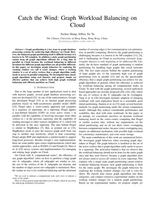
Abstract— <str<strong>on</strong>g>Graph</str<strong>on</strong>g> partiti<strong>on</strong>ing is a key issue in graph database<br />
processing systems for achieving high efficiency <strong>on</strong> <strong>Cloud</strong>. However,<br />
<str<strong>on</strong>g>the</str<strong>on</strong>g> balanced graph partiti<strong>on</strong>ing itself is difficult because it is<br />
known to be NP-complete. In additi<strong>on</strong> a static graph partiti<strong>on</strong>ing<br />
cannot keep all graph algorithms efficient for a l<strong>on</strong>g time in<br />
parallel <strong>on</strong> <strong>Cloud</strong> because <str<strong>on</strong>g>the</str<strong>on</strong>g> workload balancing in different<br />
iterati<strong>on</strong>s for different graph algorithms are all possible different.<br />
In this paper, we investigate graph behaviors by exploring <str<strong>on</strong>g>the</str<strong>on</strong>g><br />
working window (we call it wind) changes, where a working<br />
window is a set of active vertices that a graph algorithm really<br />
needs to access in parallel computing. We investigated nine classic<br />
graph algorithms using real datasets, and propose simple yet<br />
effective policies that can achieve both high graph workload<br />
balancing and efficient partiti<strong>on</strong> <strong>on</strong> <strong>Cloud</strong>.<br />
I. INTRODUCTION<br />
Due to <str<strong>on</strong>g>the</str<strong>on</strong>g> large number of new applicati<strong>on</strong>s need to deal<br />
with massive graphs, several graph database processing systems<br />
are developed [22]. As <strong>on</strong>e of <str<strong>on</strong>g>the</str<strong>on</strong>g> representatives, Google<br />
has developed Pregel [15] as its internal graph processing<br />
platform based <strong>on</strong> bulk-synchr<strong>on</strong>ous parallel model (BSP)<br />
[25]. Pregel takes a vertex-centric approach and computes<br />
in a sequence of supersteps. In a superstep, Pregel applies<br />
a user-defined functi<strong>on</strong> (UDF) <strong>on</strong> every active vertex v in<br />
parallel, with <str<strong>on</strong>g>the</str<strong>on</strong>g> capability of receiving messages from o<str<strong>on</strong>g>the</str<strong>on</strong>g>r<br />
vertices to v in <str<strong>on</strong>g>the</str<strong>on</strong>g> previous superstep, and <str<strong>on</strong>g>the</str<strong>on</strong>g> capability of<br />
sending messages to o<str<strong>on</strong>g>the</str<strong>on</strong>g>r vertices (neighbors of v), which will<br />
be delivered in <str<strong>on</strong>g>the</str<strong>on</strong>g> next superstep. The idea behind Pregel<br />
is similar to MapReduce [7]. But, as pointed out in [15],<br />
MapReduce needs to pass <str<strong>on</strong>g>the</str<strong>on</strong>g> massive graph itself from <strong>on</strong>e<br />
step to ano<str<strong>on</strong>g>the</str<strong>on</strong>g>r step iteratively, which is time c<strong>on</strong>suming.<br />
Pregel adopts BSP and implements a stateful model to support<br />
l<strong>on</strong>g-lived processes. Besides Google’s own implementati<strong>on</strong>,<br />
<str<strong>on</strong>g>the</str<strong>on</strong>g>re are some public open source implementati<strong>on</strong>s which take<br />
similar approaches, such as HAMA [1] and Giraph [2]. Shao et<br />
al. in [22] survey systems and implementati<strong>on</strong>s for managing<br />
and mining large graphs <strong>on</strong> <strong>Cloud</strong>.<br />
On <strong>Cloud</strong> with K computati<strong>on</strong>al nodes 1 , <str<strong>on</strong>g>the</str<strong>on</strong>g> efficiency of<br />
any graph algorithm 2 relies <strong>on</strong> how to partiti<strong>on</strong> a large graph<br />
into K subgraphs, where all subgraphs are similar in size,<br />
<str<strong>on</strong>g>the</str<strong>on</strong>g> sets of <str<strong>on</strong>g>the</str<strong>on</strong>g> vertices of <str<strong>on</strong>g>the</str<strong>on</strong>g> K subgraphs are disjoint, and<br />
<str<strong>on</strong>g>the</str<strong>on</strong>g> number of edges across two subgraphs is minimized. Here,<br />
<str<strong>on</strong>g>the</str<strong>on</strong>g> similar in size is for workload balancing and <str<strong>on</strong>g>the</str<strong>on</strong>g> minimum<br />
1 We use node to indicate a computati<strong>on</strong>al node, and vertex to indicate a<br />
vertex in <str<strong>on</strong>g>the</str<strong>on</strong>g> graph<br />
2 Here we mean general graph algorithms run <strong>on</strong> Pregel, which do not aware<br />
<str<strong>on</strong>g>the</str<strong>on</strong>g> underlying distributed envir<strong>on</strong>ment<br />
Zechao Shang, Jeffrey Xu Yu<br />
The Chinese University of H<strong>on</strong>g K<strong>on</strong>g, H<strong>on</strong>g K<strong>on</strong>g, China<br />
{zcshang,yu}@se.cuhk.edu.hk<br />
number of crossing edges is for communicati<strong>on</strong> cost minimizati<strong>on</strong>,<br />
in parallel computing. However, <str<strong>on</strong>g>the</str<strong>on</strong>g> graph partiti<strong>on</strong>ing is<br />
challenging because it is known to be NP-complete [11], [4],<br />
and is challenging <strong>on</strong> <strong>Cloud</strong> as partiti<strong>on</strong>ing extremely large,<br />
irregular datasets is <strong>on</strong>ly beginning to be addressed [8]. Currently,<br />
<str<strong>on</strong>g>the</str<strong>on</strong>g> de-facto standard of graph partiti<strong>on</strong>ing is random<br />
partiti<strong>on</strong>ing for handling large graphs like social networks<br />
[20]. The two main reas<strong>on</strong>s behind <str<strong>on</strong>g>the</str<strong>on</strong>g> random partiti<strong>on</strong>ing<br />
of large graphs are: (i) <str<strong>on</strong>g>the</str<strong>on</strong>g> extremely high cost of graph<br />
partiti<strong>on</strong>ing even in parallel [21] and (ii) <str<strong>on</strong>g>the</str<strong>on</strong>g> questi<strong>on</strong>able<br />
efficiency that a single graph partiti<strong>on</strong>ing can achieve for any<br />
graph algorithms in general, where <str<strong>on</strong>g>the</str<strong>on</strong>g> efficiency is achieved<br />
by workload balancing am<strong>on</strong>g all computati<strong>on</strong>al nodes <strong>on</strong><br />
<strong>Cloud</strong>. To deal with <str<strong>on</strong>g>the</str<strong>on</strong>g> graph partiti<strong>on</strong>ing, several replicati<strong>on</strong><br />
based approaches are recently proposed [20], [16], [26], where<br />
<str<strong>on</strong>g>the</str<strong>on</strong>g> sets of vertices in <str<strong>on</strong>g>the</str<strong>on</strong>g> K subgraphs can be overlapped.<br />
Yang et al. in [26] investigate dynamic adapti<strong>on</strong> of changing<br />
workload with such replicati<strong>on</strong> based <strong>on</strong> a reas<strong>on</strong>able good<br />
initial partiti<strong>on</strong>ing. Stant<strong>on</strong> et al. in [23] study several heuristic<br />
methods for graph partiti<strong>on</strong>ing under <str<strong>on</strong>g>the</str<strong>on</strong>g> stream computati<strong>on</strong><br />
model. Although <str<strong>on</strong>g>the</str<strong>on</strong>g>y achieve c<strong>on</strong>siderable performance and<br />
scalability, <str<strong>on</strong>g>the</str<strong>on</strong>g>y deal with static workloads. In this paper, as<br />
an attempt, we c<strong>on</strong>centrate ourselves <strong>on</strong> dynamic workload<br />
balancing based <strong>on</strong> <str<strong>on</strong>g>the</str<strong>on</strong>g> vertex-centric computing that Pregel<br />
or similar systems take, without any requirements <strong>on</strong> <str<strong>on</strong>g>the</str<strong>on</strong>g><br />
initial partiti<strong>on</strong>ing, and we do not allow vertex overlapping<br />
between computati<strong>on</strong>al nodes, because vertex overlapping may<br />
require an additi<strong>on</strong>al mechanism with possible high overhead<br />
for c<strong>on</strong>sistency maintenance, and costs more storage.<br />
The main c<strong>on</strong>tributi<strong>on</strong>s of this work are summarized below.<br />
We investigate graph behaviors when executing graph algorithms<br />
in Pregel. The graph behavior is modeled as <str<strong>on</strong>g>the</str<strong>on</strong>g> set of<br />
<str<strong>on</strong>g>the</str<strong>on</strong>g> active vertices that a graph algorithm really needs to access<br />
in a superstep. The motivati<strong>on</strong> behind is that we observe that<br />
<str<strong>on</strong>g>the</str<strong>on</strong>g> workload balancing should not be d<strong>on</strong>e for <str<strong>on</strong>g>the</str<strong>on</strong>g> entire graph<br />
<strong>on</strong>ce and thus used forever, because a graph algorithm does<br />
not always need to access all vertices in every superstep. This<br />
explains why a single static graph partiti<strong>on</strong>ing cannot achieve<br />
workload balancing because such graph partiti<strong>on</strong>ing is built<br />
for <str<strong>on</strong>g>the</str<strong>on</strong>g> entire graph. We investigate <str<strong>on</strong>g>the</str<strong>on</strong>g> graph behaviors by<br />
exploring <str<strong>on</strong>g>the</str<strong>on</strong>g> working window changes (we call it wind for<br />
short). We classify nine classic graph algorithms into three<br />
categories, and c<strong>on</strong>duct extensive experimental studies <strong>on</strong> <str<strong>on</strong>g>the</str<strong>on</strong>g><br />
working window changes for a random graph partiti<strong>on</strong>ing.<br />
Based <strong>on</strong> our experimental studies, we propose simple yet
effective policies that can achieve workload balancing for <str<strong>on</strong>g>the</str<strong>on</strong>g><br />
active vertices and reduce <str<strong>on</strong>g>the</str<strong>on</strong>g> number of edges across different<br />
computati<strong>on</strong>al nodes in supersteps starting from an initial<br />
random graph partiti<strong>on</strong>ing. We c<strong>on</strong>firm <str<strong>on</strong>g>the</str<strong>on</strong>g> effectiveness and<br />
<str<strong>on</strong>g>the</str<strong>on</strong>g> efficiency of our policies <strong>on</strong> a prototyped system we have<br />
built <strong>on</strong> top of HAMA [1], an open source implementati<strong>on</strong> of<br />
Pregel.<br />
The remainder of <str<strong>on</strong>g>the</str<strong>on</strong>g> paper is organized as follows. We<br />
discuss Pregel in Secti<strong>on</strong> II <strong>on</strong> which our prototyped system is<br />
built up, and discuss nine graph algorithms in three categories<br />
to which we investigate how to support dynamic workload<br />
balancing in Secti<strong>on</strong> III. We show our experimental studies in<br />
Secti<strong>on</strong> V. We discuss <str<strong>on</strong>g>the</str<strong>on</strong>g> related work <strong>on</strong> graph partiti<strong>on</strong>ing<br />
in Secti<strong>on</strong> VI, and c<strong>on</strong>clude our paper in Secti<strong>on</strong> VII.<br />
II. THE PREGEL<br />
Google has developed Pregel [15] as its internal graph<br />
processing platform based <strong>on</strong> bulk-synchr<strong>on</strong>ous parallel model<br />
BSP [25]. Pregel distributes data <strong>on</strong> all computati<strong>on</strong>al nodes,<br />
and during <str<strong>on</strong>g>the</str<strong>on</strong>g> entire computing all data are assumed to reside<br />
in main memory. Pregel takes a vertex-centric approach and<br />
computes in a sequence of supersteps. In each superstep, every<br />
node in Pregel computes a user-defined functi<strong>on</strong> (UDF) against<br />
each vertex in a graph in parallel. The UDF computes u’s<br />
value based <strong>on</strong> <str<strong>on</strong>g>the</str<strong>on</strong>g> receiving messages to u, which are sent<br />
from o<str<strong>on</strong>g>the</str<strong>on</strong>g>r vertices in <str<strong>on</strong>g>the</str<strong>on</strong>g> previous superstep, and <str<strong>on</strong>g>the</str<strong>on</strong>g> UDF<br />
may also send messages from u to o<str<strong>on</strong>g>the</str<strong>on</strong>g>r vertices (neighbors<br />
of u) which will receive <str<strong>on</strong>g>the</str<strong>on</strong>g> messages in <str<strong>on</strong>g>the</str<strong>on</strong>g> next superstep.<br />
In general, a vertex u can receive/send messages from/to its<br />
neighbors which reside in <str<strong>on</strong>g>the</str<strong>on</strong>g> same or different nodes. The<br />
synchr<strong>on</strong>izati<strong>on</strong> is d<strong>on</strong>e at <str<strong>on</strong>g>the</str<strong>on</strong>g> end of every superstep to ensure<br />
that all nodes complete <str<strong>on</strong>g>the</str<strong>on</strong>g>ir tasks (including sending/receiving<br />
messages) before entering <str<strong>on</strong>g>the</str<strong>on</strong>g> next superstep.<br />
Pregel hides <str<strong>on</strong>g>the</str<strong>on</strong>g> underlying communicati<strong>on</strong> mechanism<br />
completely. The applicati<strong>on</strong> to be built <strong>on</strong> top of Pregel<br />
cannot c<strong>on</strong>trol any low level operati<strong>on</strong>s such as mode of sending/receiving<br />
messages, workload balancing, data partiti<strong>on</strong> and<br />
replicati<strong>on</strong>.<br />
Some functi<strong>on</strong>s provided in <str<strong>on</strong>g>the</str<strong>on</strong>g> vertex-centric API in Pregel<br />
are shown below for accessing vertices.<br />
class Vertex {<br />
VertexValue getVertexValue();<br />
void setVertexValue(Value);<br />
int getSuperStep();<br />
void SendMessageTo(Vertex, MessageValue);<br />
void VoteToHalt();<br />
void abstract UDF (MessageIterator);<br />
}<br />
Here, getVertexValue() and setVertexValue() get/set <str<strong>on</strong>g>the</str<strong>on</strong>g> vertex<br />
value, respectively. SendMessageTo() takes two inputs: <str<strong>on</strong>g>the</str<strong>on</strong>g><br />
vertex to be sent and <str<strong>on</strong>g>the</str<strong>on</strong>g> message to be delivered. getSuper-<br />
Step() gets <str<strong>on</strong>g>the</str<strong>on</strong>g> current superstep number. UDF is <str<strong>on</strong>g>the</str<strong>on</strong>g> functi<strong>on</strong><br />
to be implemented by an applicati<strong>on</strong>. The input to UDF is<br />
a MessageIterator, which is used to access every receiving<br />
messages to <str<strong>on</strong>g>the</str<strong>on</strong>g> corresp<strong>on</strong>ding vertex. In <str<strong>on</strong>g>the</str<strong>on</strong>g> following, for<br />
simplicity, for a vertex u, we take <str<strong>on</strong>g>the</str<strong>on</strong>g> MessageIterator as a<br />
set of messages to u denoted as Mu. Any vertex is initially<br />
set as active, and becomes inactive by calling VoteToHalt() by<br />
Algorithm 1: A Computati<strong>on</strong>al Node in Pregel<br />
1 foreach active vertex u do<br />
2 u.UDF (received messages to u from <str<strong>on</strong>g>the</str<strong>on</strong>g> previous<br />
superstep);<br />
3 send out all outgoing messages;<br />
4 enter barrier (all nodes wait here for sync);<br />
TABLE I<br />
SUMMARY OF THE NINE GRAPH ALGORITHMS<br />
No. Algorithm Category<br />
A1 PageRank [15], [17]<br />
A2 Semi-clustering [15]<br />
I<br />
A3 <str<strong>on</strong>g>Graph</str<strong>on</strong>g> Coloring [19], [13]<br />
A4 Single Source Shortest Path (SSSP) [15], [5]<br />
A5 Breadth First Search (BFS) [6]<br />
II<br />
A6 Random-Walk [18]<br />
A7 Maximal Matching (MM) [15], [3]<br />
A8 Minimum Spanning Tree (MST) [19], [10] III<br />
A9 Maximal Independent Sets (MIS) [19], [14]<br />
<str<strong>on</strong>g>the</str<strong>on</strong>g> vertex itself. An inactive vertex will become active again<br />
when it receives message(s). The Pregel repeats <str<strong>on</strong>g>the</str<strong>on</strong>g> supersteps<br />
until all vertices become inactive.<br />
Algorithm 1 depicts a node in Pregel. In <str<strong>on</strong>g>the</str<strong>on</strong>g> for loop, it<br />
computes <str<strong>on</strong>g>the</str<strong>on</strong>g> UDF for each active vertex u in a superstep,<br />
and <str<strong>on</strong>g>the</str<strong>on</strong>g>n sends out all messages from a vertex that requests.<br />
The sending (line 3) in Algorithm 1 is completely different<br />
from <str<strong>on</strong>g>the</str<strong>on</strong>g> member functi<strong>on</strong> of SendMessageTo() in <str<strong>on</strong>g>the</str<strong>on</strong>g> Vertex<br />
class. The latter is to highlight that it needs to send messages<br />
and <str<strong>on</strong>g>the</str<strong>on</strong>g> former is <str<strong>on</strong>g>the</str<strong>on</strong>g> <strong>on</strong>e that really sends messages. Besides<br />
Google’s own implementati<strong>on</strong>, <str<strong>on</strong>g>the</str<strong>on</strong>g>re are some public open<br />
source implementati<strong>on</strong>s which take <str<strong>on</strong>g>the</str<strong>on</strong>g> similar approaches,<br />
such as HAMA [1] and Giraph [2].<br />
III. NINE GRAPH ALGORITHMS<br />
We discuss nine classic graph algorithms including PageRank<br />
[15], [17], Semi-clustering [15], <str<strong>on</strong>g>Graph</str<strong>on</strong>g> Coloring [19],<br />
[13], Single Source Shortest Path (SSSP) [15], [5], Breadth<br />
First Search (BFS) [6], Random-Walk [18], Maximal Matching<br />
(MM) [15], [3], Minimum Spanning Tree (MST) [19], [10],<br />
and Maximal Independent Sets (MIS) [19], [14]. In <str<strong>on</strong>g>the</str<strong>on</strong>g> Pregel<br />
framework, all graph algorithms need to implement a vertexcentric<br />
UDF functi<strong>on</strong> as indicated in line 2 in Algorithm 1. We<br />
divide all <str<strong>on</strong>g>the</str<strong>on</strong>g> 9 graph algorithms into 3 categories by <str<strong>on</strong>g>the</str<strong>on</strong>g> ways<br />
of a UDF functi<strong>on</strong> being designed, namely, Always-Active-<br />
Style, Traversal-Style, and Multi-Phase-Style. We discuss <str<strong>on</strong>g>the</str<strong>on</strong>g>m<br />
below.<br />
Always-Active-Style (Category I): By Always-Active-Style,<br />
every vertex in every superstep sends messages to all its<br />
neighbors. The main steps are illustrated in Algorithm 2.<br />
Here, <str<strong>on</strong>g>the</str<strong>on</strong>g> UDF functi<strong>on</strong> defined <strong>on</strong> a vertex u receives a<br />
set of messages Mu, which were sent to u in <str<strong>on</strong>g>the</str<strong>on</strong>g> immediate<br />
previous superstep by <str<strong>on</strong>g>the</str<strong>on</strong>g> neighbors of u. The UDF functi<strong>on</strong><br />
first computes <str<strong>on</strong>g>the</str<strong>on</strong>g> value of u based <strong>on</strong> both <str<strong>on</strong>g>the</str<strong>on</strong>g> old value that u<br />
holds and <str<strong>on</strong>g>the</str<strong>on</strong>g> messages received (line 1). Then, it will inform<br />
all u’s neighbors of <str<strong>on</strong>g>the</str<strong>on</strong>g> current value of u (line 2-3), and also
Algorithm 2: Always-Active-Style (Mu)<br />
Input: Mu, all incoming messages to vertex u<br />
1 Call an aggregate functi<strong>on</strong> <strong>on</strong> u based <strong>on</strong> Mu;<br />
2 foreach outgoing edge e = (u, v) do<br />
3 Send a message to v;<br />
4 Change <str<strong>on</strong>g>the</str<strong>on</strong>g> local vertex value <strong>on</strong> u if necessary;<br />
Algorithm 3: PageRank-UDF<br />
Input: Mu, all incoming messages to vertex u<br />
1 sum ← 0;<br />
2 foreach message m ∈ Mu do<br />
3 sum ← sum + m;<br />
4 p ← u’s value;<br />
5 p ← α · p + (1 − α) · sum;<br />
6 foreach outgoing edge e = (u, v) from u do<br />
7 Send a message with value p/degree(u) to vertex v;<br />
8 Set u’s value to be p;<br />
update <str<strong>on</strong>g>the</str<strong>on</strong>g> current value of u to be held for <str<strong>on</strong>g>the</str<strong>on</strong>g> next superstep<br />
(line 4). PageRank, Semi-clustering, and <str<strong>on</strong>g>Graph</str<strong>on</strong>g> Coloring are<br />
all in this category.<br />
As an example, <str<strong>on</strong>g>the</str<strong>on</strong>g> vertex-centric PageRank UDF is shown<br />
in Algorithm 3 based <strong>on</strong> Pregel implementati<strong>on</strong> [15]. Every<br />
vertex is assigned to an initial value, which is its initial<br />
rank. The UDF functi<strong>on</strong> computes a new rank at <str<strong>on</strong>g>the</str<strong>on</strong>g> i-th<br />
superstep for vertex u by combining its previous rank and<br />
<str<strong>on</strong>g>the</str<strong>on</strong>g> aggregati<strong>on</strong> of <str<strong>on</strong>g>the</str<strong>on</strong>g> ranks of its neighbors (line 1-5). It <str<strong>on</strong>g>the</str<strong>on</strong>g>n<br />
sends <str<strong>on</strong>g>the</str<strong>on</strong>g> new rank of u to its neighbors (line 6-7), and sets <str<strong>on</strong>g>the</str<strong>on</strong>g><br />
new rank of u to be held for <str<strong>on</strong>g>the</str<strong>on</strong>g> next iterati<strong>on</strong>. The terminati<strong>on</strong><br />
c<strong>on</strong>diti<strong>on</strong> is based <strong>on</strong> <str<strong>on</strong>g>the</str<strong>on</strong>g> pre-determined number of supersteps,<br />
and all nodes will terminate at <str<strong>on</strong>g>the</str<strong>on</strong>g> same time. It is important to<br />
notice that all vertices are active sending <str<strong>on</strong>g>the</str<strong>on</strong>g>ir updated ranks<br />
to <str<strong>on</strong>g>the</str<strong>on</strong>g>ir neighbors, because such rank values have impacts <strong>on</strong><br />
<str<strong>on</strong>g>the</str<strong>on</strong>g> ranks of <str<strong>on</strong>g>the</str<strong>on</strong>g>ir neighbors, and <str<strong>on</strong>g>the</str<strong>on</strong>g>ir neighbors’ neighbors,<br />
etc.<br />
Traversal-Style (Category II): By Traversal-Style, a specific<br />
vertex is treated as a starting point, and <str<strong>on</strong>g>the</str<strong>on</strong>g> o<str<strong>on</strong>g>the</str<strong>on</strong>g>r vertices<br />
are involved in computing based <strong>on</strong> how it propagates <strong>on</strong><br />
c<strong>on</strong>diti<strong>on</strong>s. The main steps are illustrated in Algorithm 4.<br />
Initially, <strong>on</strong>ly <strong>on</strong>e vertex will be set as active and all o<str<strong>on</strong>g>the</str<strong>on</strong>g>rs are<br />
in <str<strong>on</strong>g>the</str<strong>on</strong>g> inactive status. In <str<strong>on</strong>g>the</str<strong>on</strong>g> computing, a vertex u becomes<br />
active when it receives some messages (Mu). As shown in<br />
Algorithm 4, <str<strong>on</strong>g>the</str<strong>on</strong>g> UDF functi<strong>on</strong> updates <str<strong>on</strong>g>the</str<strong>on</strong>g> value of u based <strong>on</strong><br />
<str<strong>on</strong>g>the</str<strong>on</strong>g> messages received (line 1-2). If <str<strong>on</strong>g>the</str<strong>on</strong>g> value of u is updated,<br />
it implies that it is now involved in <str<strong>on</strong>g>the</str<strong>on</strong>g> computing of <str<strong>on</strong>g>the</str<strong>on</strong>g><br />
given graph algorithm, and it will propagate to some of its<br />
selected neighbors <strong>on</strong> c<strong>on</strong>diti<strong>on</strong>s (line 4-5). Because u does not<br />
necessarily need to be involved in <str<strong>on</strong>g>the</str<strong>on</strong>g> computing all <str<strong>on</strong>g>the</str<strong>on</strong>g> time,<br />
u will vote to halt by calling <str<strong>on</strong>g>the</str<strong>on</strong>g> member functi<strong>on</strong> VoteToHalt()<br />
to voluntarily be inactive (line 7). Note that a vertex will be<br />
waked up by <str<strong>on</strong>g>the</str<strong>on</strong>g> messages received. It is interesting to note<br />
that <str<strong>on</strong>g>the</str<strong>on</strong>g> category I algorithms, for example PageRank, cannot<br />
effectively use VoteToHalt(), because <str<strong>on</strong>g>the</str<strong>on</strong>g> value of a vertex will<br />
Algorithm 4: Traversal-Style (Mu)<br />
Input: Mu, all incoming messages to vertex u<br />
1 Call an aggregate functi<strong>on</strong> <strong>on</strong> u based <strong>on</strong> Mu;<br />
2 Update <str<strong>on</strong>g>the</str<strong>on</strong>g> vertex value for u if needed;<br />
3 if u’s vertex value is updated <str<strong>on</strong>g>the</str<strong>on</strong>g>n<br />
4 foreach outgoing edge e = (u, v) do<br />
5 Send a message to v <strong>on</strong> c<strong>on</strong>diti<strong>on</strong>;<br />
6 Set <str<strong>on</strong>g>the</str<strong>on</strong>g> local vertex value <strong>on</strong> u if needed;<br />
7 VoteToHalt();<br />
Algorithm 5: SSSP-UDF<br />
Input: Mu, all incoming messages to vertex u<br />
1 dmin ← ∞;<br />
2 foreach message m ∈ Mu do<br />
3 dmin ← min(m, dmin);<br />
4 p ← u’s value;<br />
5 if dmin < p <str<strong>on</strong>g>the</str<strong>on</strong>g>n<br />
6 foreach outgoing edge e = (u, v) from u do<br />
7 Send a message to v, with a value of dmin + ω(u, v);<br />
8 Set u’s local value as dmin;<br />
9 VoteToHalt();<br />
always affect o<str<strong>on</strong>g>the</str<strong>on</strong>g>rs, even if <str<strong>on</strong>g>the</str<strong>on</strong>g> value of <str<strong>on</strong>g>the</str<strong>on</strong>g> vertex satisfies<br />
<str<strong>on</strong>g>the</str<strong>on</strong>g> c<strong>on</strong>verge c<strong>on</strong>diti<strong>on</strong>, for example, <str<strong>on</strong>g>the</str<strong>on</strong>g> error bound between<br />
<str<strong>on</strong>g>the</str<strong>on</strong>g> current value and its previous value is less than or equal to<br />
a threshold. Typical algorithms in <str<strong>on</strong>g>the</str<strong>on</strong>g> category II are Breadth<br />
First Search [6], Single Source Shortest Path [6], and Random-<br />
Walk [18].<br />
The implementati<strong>on</strong> of SSSP is illustrated in Algorithm 5.<br />
Initially every vertex u, except <str<strong>on</strong>g>the</str<strong>on</strong>g> start vertex, is assigned to<br />
an initial value ∞ for <str<strong>on</strong>g>the</str<strong>on</strong>g> shortest distance from <str<strong>on</strong>g>the</str<strong>on</strong>g> starting<br />
vertex to u. In SSSP, a vertex u receives messages from some<br />
of its neighbors if some of its neighbors have updated <str<strong>on</strong>g>the</str<strong>on</strong>g>ir<br />
shortest distance from <str<strong>on</strong>g>the</str<strong>on</strong>g> starting vertex. The UDF functi<strong>on</strong><br />
will determine <str<strong>on</strong>g>the</str<strong>on</strong>g> new shortest distance from <str<strong>on</strong>g>the</str<strong>on</strong>g> starting<br />
vertex to u itself via some of u’s neighbors (line 1-3). If <str<strong>on</strong>g>the</str<strong>on</strong>g><br />
new shortest distance becomes smaller, u will send messages<br />
to its neighbors to tell <str<strong>on</strong>g>the</str<strong>on</strong>g>m <str<strong>on</strong>g>the</str<strong>on</strong>g> new updates (line 6-7), where<br />
ω(u, v) is <str<strong>on</strong>g>the</str<strong>on</strong>g> edge weight <strong>on</strong> <str<strong>on</strong>g>the</str<strong>on</strong>g> edge from u to its neighbor<br />
v. Because u may not necessarily need to be involved in <str<strong>on</strong>g>the</str<strong>on</strong>g><br />
shortest distance computing, it votes to halt (line 9).<br />
Multi-Phase-Style (Category III): As illustrated in Algorithm<br />
6, a single phase, for example, to identify <strong>on</strong>e matching<br />
edge am<strong>on</strong>g many, cannot be d<strong>on</strong>e in a single superstep,<br />
because a matching edge is an edge (u, v) that nei<str<strong>on</strong>g>the</str<strong>on</strong>g>r u nor<br />
v is involved in ano<str<strong>on</strong>g>the</str<strong>on</strong>g>r matching edge. It needs to be d<strong>on</strong>e in<br />
several supersteps in Pregel. The entire computati<strong>on</strong> is divided<br />
into a number of phases, and each phase, Pj is d<strong>on</strong>e in k<br />
supersteps: Pj0, Pj1, · · · , Pji, · · · , Pik−1 . Typical algorithms<br />
in <str<strong>on</strong>g>the</str<strong>on</strong>g> category III are MM [15], [3], MST [19], [10], and<br />
MIS [19], [14].<br />
We discuss <str<strong>on</strong>g>the</str<strong>on</strong>g> maximal matching problem (MM), as an<br />
example, which is to find a maximal subset of edges, ME,
Algorithm 6: Multi-Phase-Style (Mu)<br />
Input: Mu, all incoming messages to vertex u<br />
1 if u has completed its computing <str<strong>on</strong>g>the</str<strong>on</strong>g>n<br />
2 VoteToHalt(); return;<br />
3 switch getSuperStep() % k do<br />
4 ...;<br />
5 case i /* 0 ≤ i < k */<br />
6 call ei<str<strong>on</strong>g>the</str<strong>on</strong>g>r Always-Active-Style or Traversal-Style style<br />
UDF; break;<br />
7 ...;<br />
Algorithm 7: MM-UDF<br />
Input: Mu, all incoming messages to vertex u<br />
1 if u itself is a matched point <str<strong>on</strong>g>the</str<strong>on</strong>g>n<br />
2 VoteToHalt(); return;<br />
3 switch getSuperStep() % 4 do<br />
4 case 0 /* invitati<strong>on</strong> */<br />
5 foreach outgoing edge e = (u, v) from u do<br />
6 Send a message to v to invite ;<br />
7 acceptu ← false;<br />
8 break;<br />
9 case 1 /* acceptance */<br />
10 Randomly pick an edge e = (u, v) up from Mu;<br />
11 Send a message to v to accept; acceptu ← true; break;<br />
12 case 2 /* c<strong>on</strong>firmati<strong>on</strong> */<br />
13 if acceptu = false <str<strong>on</strong>g>the</str<strong>on</strong>g>n<br />
14 Randomly pick an edge e = (u, v) up from Mu;<br />
15 Send a message to v to c<strong>on</strong>firm;<br />
16 Set u as a matched point; VoteToHalt(); break;<br />
17 case 3 /* marking */<br />
18 if Mu = ∅ <str<strong>on</strong>g>the</str<strong>on</strong>g>n<br />
19 Set u as a matched point; VoteToHalt(); break;<br />
in a given graph G where no two edges in ME have a<br />
comm<strong>on</strong> vertex. In Pregel, a randomized algorithm [3] is<br />
used to support a bipartite maximal matching, which can be<br />
extended to handle maximal matching in general graph. The<br />
computati<strong>on</strong> is divided into a number of phases, and each<br />
phase, Pi, is d<strong>on</strong>e in four supersteps, namely, Pi0 , Pi1 , Pi2 ,<br />
and Pi3 . In Pi0 , all vertices that have not been involved in any<br />
matching send a message to <str<strong>on</strong>g>the</str<strong>on</strong>g>ir neighbors to invite <str<strong>on</strong>g>the</str<strong>on</strong>g>m to<br />
join a match. In Pi1 , a vertex randomly accepts <strong>on</strong>e of <str<strong>on</strong>g>the</str<strong>on</strong>g><br />
invitati<strong>on</strong>s to join a matching, and replies <str<strong>on</strong>g>the</str<strong>on</strong>g> corresp<strong>on</strong>ding<br />
sender a message, because a vertex may possibly receive many<br />
matching invitati<strong>on</strong>s from its neighbors. In Pi2 , in a similar<br />
fashi<strong>on</strong>, a vertex that has sent invitati<strong>on</strong>s may receive several<br />
acceptances, and will c<strong>on</strong>firm <strong>on</strong>e acceptance by replying a<br />
message. In Pi3, <str<strong>on</strong>g>the</str<strong>on</strong>g> vertex that receives a c<strong>on</strong>firmati<strong>on</strong> will<br />
mark itself as marked. The computati<strong>on</strong> repeats until no more<br />
matches can be identified. As illustrated in Algorithm 7, <strong>on</strong>e<br />
important thing is that a vertex may not resp<strong>on</strong>d to any when<br />
it has already been matched.<br />
IV. SUPER-DYNAMIC PARTITIONING<br />
In this secti<strong>on</strong>, we discuss two important issues which are<br />
also c<strong>on</strong>flict with each o<str<strong>on</strong>g>the</str<strong>on</strong>g>r in Pregel-like systems for large<br />
graph processing. The two issues are workload balancing and<br />
communicati<strong>on</strong> cost minimizati<strong>on</strong>. In Pregel, <str<strong>on</strong>g>the</str<strong>on</strong>g> number of<br />
vertices is <str<strong>on</strong>g>the</str<strong>on</strong>g> dominant factor for workload in each computati<strong>on</strong>al<br />
node, because of its vertex-centric computing. The<br />
workload balancing suggests that all nodes are best to have<br />
similar amount of workload in every superstep. The intuiti<strong>on</strong><br />
is that <str<strong>on</strong>g>the</str<strong>on</strong>g> computing cost of a superstep is <str<strong>on</strong>g>the</str<strong>on</strong>g> max computing<br />
cost of <str<strong>on</strong>g>the</str<strong>on</strong>g> node that has <str<strong>on</strong>g>the</str<strong>on</strong>g> largest workload. <str<strong>on</strong>g>Workload</str<strong>on</strong>g><br />
balancing will lead to minimizati<strong>on</strong> of computati<strong>on</strong>al cost<br />
of supersteps. On <str<strong>on</strong>g>the</str<strong>on</strong>g> o<str<strong>on</strong>g>the</str<strong>on</strong>g>r hand, <str<strong>on</strong>g>the</str<strong>on</strong>g> communicati<strong>on</strong> cost<br />
minimizati<strong>on</strong> suggests that <str<strong>on</strong>g>the</str<strong>on</strong>g> communicati<strong>on</strong> cost am<strong>on</strong>g<br />
supersteps shall be minimized. It is worth noting that, in graph<br />
processing in Pregel, such communicati<strong>on</strong> cost depends <strong>on</strong><br />
<str<strong>on</strong>g>the</str<strong>on</strong>g> number of messages across computati<strong>on</strong>al nodes, and <str<strong>on</strong>g>the</str<strong>on</strong>g><br />
number of messages is heavily dependent <strong>on</strong> <str<strong>on</strong>g>the</str<strong>on</strong>g> number of<br />
edges that cross different computati<strong>on</strong>al nodes. Minimizing<br />
<str<strong>on</strong>g>the</str<strong>on</strong>g> communicati<strong>on</strong> cost will significantly reduce <str<strong>on</strong>g>the</str<strong>on</strong>g> time for<br />
synchr<strong>on</strong>izati<strong>on</strong>. The two issues are important, because <str<strong>on</strong>g>the</str<strong>on</strong>g><br />
system excuti<strong>on</strong> time depends <strong>on</strong> both of <str<strong>on</strong>g>the</str<strong>on</strong>g>m. The two issues<br />
are c<strong>on</strong>flict. First, balancing workload am<strong>on</strong>g computati<strong>on</strong>al<br />
nodes may increase <str<strong>on</strong>g>the</str<strong>on</strong>g> number of edges that are across<br />
different computati<strong>on</strong>al nodes which leads to possibly high<br />
communicati<strong>on</strong> cost. Sec<strong>on</strong>d, minimizing <str<strong>on</strong>g>the</str<strong>on</strong>g> communicati<strong>on</strong><br />
cost may make all workload goes to a single computati<strong>on</strong>al<br />
node.<br />
<str<strong>on</strong>g>Graph</str<strong>on</strong>g> Notati<strong>on</strong>s: C<strong>on</strong>sider a graph G = (V, E), where V<br />
is <str<strong>on</strong>g>the</str<strong>on</strong>g> set of vertices, and E ⊆ V × V is <str<strong>on</strong>g>the</str<strong>on</strong>g> set of directed<br />
edges. We use n = |V |, m = |E| to denote <str<strong>on</strong>g>the</str<strong>on</strong>g> numbers of<br />
vertices and edges, respectively.<br />
A graph G will be distributed to <str<strong>on</strong>g>the</str<strong>on</strong>g> K computati<strong>on</strong>al nodes,<br />
{N1, N2, · · · , NK}, in Pregel for parallel processing, where<br />
all Ni have <str<strong>on</strong>g>the</str<strong>on</strong>g> same memory capacity C.<br />
At <str<strong>on</strong>g>the</str<strong>on</strong>g> s-th superstep, each node Ni holds a subset of<br />
vertices, V s<br />
s s<br />
i ⊆ V under <str<strong>on</strong>g>the</str<strong>on</strong>g> c<strong>on</strong>diti<strong>on</strong> that Vi ∩ Vj = ∅<br />
for (i = j) and V = V s<br />
i , and holds a subset of internal<br />
edges, IE s i = {(u, v)|(u, v) ∈ E, u ∈ V s<br />
s<br />
i , v ∈ Vi }. The<br />
edges that cross nodes are called external edges. We use EE s i,j<br />
to denote <str<strong>on</strong>g>the</str<strong>on</strong>g> set of external edges which cross two different<br />
computati<strong>on</strong>al nodes, Ni and Nj, i = j, such as EE s i,j =<br />
{(u, v)|(u, v) ∈ E, u ∈ V s<br />
s<br />
i , v ∈ Vj } ∪ {(u, v)|(u, v) ∈<br />
E, u ∈ V s s<br />
j , v ∈ Vi }. The edges associated with partiti<strong>on</strong> Ni<br />
is Es i = ∪EEsi,j ∪ IE s i .<br />
Working <str<strong>on</strong>g>Wind</str<strong>on</strong>g>ow, <str<strong>on</strong>g>Workload</str<strong>on</strong>g>, and <str<strong>on</strong>g>Workload</str<strong>on</strong>g> <str<strong>on</strong>g>Balancing</str<strong>on</strong>g>:<br />
The computati<strong>on</strong>al cost <strong>on</strong> a computati<strong>on</strong>al node mainly<br />
depends <strong>on</strong> <str<strong>on</strong>g>the</str<strong>on</strong>g> number of active vertices that receive messages<br />
in <str<strong>on</strong>g>the</str<strong>on</strong>g> vertex-centric computing framework like Pregel. Here,<br />
<str<strong>on</strong>g>the</str<strong>on</strong>g> active vertices are a subset of <str<strong>on</strong>g>the</str<strong>on</strong>g> entire vertices in a<br />
superstep, because not all vertices will be invoked by messages<br />
in a superstep. We call <str<strong>on</strong>g>the</str<strong>on</strong>g> set of active vertices in <str<strong>on</strong>g>the</str<strong>on</strong>g> s-th<br />
superstep <strong>on</strong> a computati<strong>on</strong>al node Ni a working window, and<br />
denote it as W s i , and <str<strong>on</strong>g>the</str<strong>on</strong>g> entire working window at <str<strong>on</strong>g>the</str<strong>on</strong>g> s-th<br />
superstep is W s = ∪K i=1W s i . The average size of working
window per node at <str<strong>on</strong>g>the</str<strong>on</strong>g> s-th superstep is denoted as W s , which<br />
is computed as W s = |W s |/K.<br />
We c<strong>on</strong>sider <str<strong>on</strong>g>the</str<strong>on</strong>g> workload in <str<strong>on</strong>g>the</str<strong>on</strong>g> s-th superstep <strong>on</strong> a<br />
computati<strong>on</strong>al node Ni denoted as W s i .<br />
W s i = |W s i | + |AE s i | (1)<br />
Here, |W s i | is <str<strong>on</strong>g>the</str<strong>on</strong>g> number of active vertices <strong>on</strong> Ni, and AE s i<br />
is <str<strong>on</strong>g>the</str<strong>on</strong>g> active subset of <str<strong>on</strong>g>the</str<strong>on</strong>g> edges. The average workload in <str<strong>on</strong>g>the</str<strong>on</strong>g><br />
s-th superstep is W s = K i=1 Ws i /K.<br />
Eq. (1) indicates <str<strong>on</strong>g>the</str<strong>on</strong>g> workload depends <strong>on</strong> two factors. |W s i |<br />
is <str<strong>on</strong>g>the</str<strong>on</strong>g> number of UDF functi<strong>on</strong>s must be invoked to compute,<br />
and |AE s i | is <str<strong>on</strong>g>the</str<strong>on</strong>g> number of messages that UDF functi<strong>on</strong>s must<br />
process |W s i |. Eq. (1) takes <str<strong>on</strong>g>the</str<strong>on</strong>g> simple sum of |W s i | and |AEs i |<br />
for two reas<strong>on</strong>s. First, it is based <strong>on</strong> our observati<strong>on</strong>s. For<br />
most UDF functi<strong>on</strong>s, <str<strong>on</strong>g>the</str<strong>on</strong>g> number of computing operati<strong>on</strong>s is<br />
linear w.r.t. <str<strong>on</strong>g>the</str<strong>on</strong>g> incoming messages. Sec<strong>on</strong>d, <str<strong>on</strong>g>the</str<strong>on</strong>g> message serializati<strong>on</strong>/deserializati<strong>on</strong><br />
time is linear to <str<strong>on</strong>g>the</str<strong>on</strong>g> size of messages,<br />
which usually overtakes o<str<strong>on</strong>g>the</str<strong>on</strong>g>r operati<strong>on</strong>s and dominates <str<strong>on</strong>g>the</str<strong>on</strong>g><br />
UDF executi<strong>on</strong> time.<br />
In additi<strong>on</strong>, we use D s i,j<br />
to denote <str<strong>on</strong>g>the</str<strong>on</strong>g> number of messages<br />
sent from Ni to Nj at <str<strong>on</strong>g>the</str<strong>on</strong>g> s-th superstep, which is based <strong>on</strong><br />
EE s i,j. D s i,j implies <str<strong>on</strong>g>the</str<strong>on</strong>g> communicati<strong>on</strong> cost from Ni to Nj at<br />
<str<strong>on</strong>g>the</str<strong>on</strong>g> s-th superstep. The total communicati<strong>on</strong> cost at <str<strong>on</strong>g>the</str<strong>on</strong>g> s-th<br />
superstep is denoted as D s .<br />
Because it is very difficult to minimize <str<strong>on</strong>g>the</str<strong>on</strong>g> two objectives,<br />
namely, workload balancing and communicati<strong>on</strong> cost minimizati<strong>on</strong>,<br />
at <str<strong>on</strong>g>the</str<strong>on</strong>g> same time, in this paper, we study to minimize<br />
communicati<strong>on</strong> cost under <str<strong>on</strong>g>the</str<strong>on</strong>g> c<strong>on</strong>diti<strong>on</strong> that workloads are<br />
balanced. The problem statement is given below.<br />
Problem Statement: For a given graph algorithm expressible<br />
in Pregel, <str<strong>on</strong>g>the</str<strong>on</strong>g> problem we study is to minimize <br />
s Ds , subject<br />
to two c<strong>on</strong>diti<strong>on</strong>s in every superstep: (1) |V s<br />
i | + |Es i | ≤ C and<br />
(2) at each superstep s, all computati<strong>on</strong>al nodes are balanced,<br />
namely Ws i ≤ (1 + ɛ) × Ws , ∀i ∈ {1..K} where 0 ≤ ɛ ≪ 1.<br />
The first c<strong>on</strong>diti<strong>on</strong> suggests that a node Ni must be able to<br />
hold <str<strong>on</strong>g>the</str<strong>on</strong>g> workload assigned, and <str<strong>on</strong>g>the</str<strong>on</strong>g> sec<strong>on</strong>d c<strong>on</strong>diti<strong>on</strong> suggests<br />
that <str<strong>on</strong>g>the</str<strong>on</strong>g> workload must be balanced.<br />
The problem is challenging. First, <str<strong>on</strong>g>the</str<strong>on</strong>g> problem itself is an<br />
NP problem even in a static setting, as <str<strong>on</strong>g>the</str<strong>on</strong>g> size-balanced graph<br />
partiti<strong>on</strong> problem is shown to be NP-complete [4]. In additi<strong>on</strong>,<br />
<str<strong>on</strong>g>the</str<strong>on</strong>g> active vertices, we are most interested in, are those vertices<br />
that will be active in <str<strong>on</strong>g>the</str<strong>on</strong>g> near future ra<str<strong>on</strong>g>the</str<strong>on</strong>g>r than those vertices<br />
that are active in <str<strong>on</strong>g>the</str<strong>on</strong>g> current superstep. This is because in<br />
<str<strong>on</strong>g>the</str<strong>on</strong>g> current superstep <str<strong>on</strong>g>the</str<strong>on</strong>g> active vertices have already been<br />
determined based <strong>on</strong> <str<strong>on</strong>g>the</str<strong>on</strong>g> messages already received from<br />
<str<strong>on</strong>g>the</str<strong>on</strong>g> immediate previous superstep, and cannot be rebalanced.<br />
Sec<strong>on</strong>d, it is known to be very difficult to predict <str<strong>on</strong>g>the</str<strong>on</strong>g> workload<br />
in parallel graph processing <strong>on</strong> computati<strong>on</strong>al nodes. Third,<br />
<str<strong>on</strong>g>the</str<strong>on</strong>g>re does not exist <str<strong>on</strong>g>the</str<strong>on</strong>g> optimal graph partiti<strong>on</strong>ing under <strong>on</strong>e<br />
set of c<strong>on</strong>diti<strong>on</strong>s that can be efficiently used for any graph<br />
problems in general, for <str<strong>on</strong>g>the</str<strong>on</strong>g> reas<strong>on</strong> that <str<strong>on</strong>g>the</str<strong>on</strong>g> workloads vary<br />
greatly, as discussed for <str<strong>on</strong>g>the</str<strong>on</strong>g> 3 categories of graph algorithms.<br />
Fourth, this requests a super-dynamic soluti<strong>on</strong> during <str<strong>on</strong>g>the</str<strong>on</strong>g><br />
computati<strong>on</strong> of a graph algorithm, that must be effective and<br />
simple.<br />
1<br />
1<br />
1<br />
1<br />
2<br />
2<br />
2<br />
2<br />
3<br />
3<br />
3<br />
3<br />
5<br />
5<br />
5<br />
5<br />
4<br />
4<br />
4<br />
4<br />
6<br />
7<br />
6<br />
7<br />
6<br />
6<br />
7<br />
7<br />
8<br />
8<br />
8<br />
8<br />
11 12<br />
10<br />
11 12<br />
10<br />
9<br />
9<br />
13<br />
13<br />
11 12<br />
10<br />
9<br />
13<br />
11 12<br />
10<br />
9<br />
13<br />
14<br />
14<br />
14<br />
14<br />
(a) PageRank<br />
1<br />
2<br />
15<br />
16<br />
15<br />
16<br />
15<br />
15<br />
16<br />
16<br />
3<br />
17<br />
17<br />
5<br />
4<br />
6<br />
7<br />
8<br />
11 12<br />
10<br />
9<br />
13<br />
14<br />
15<br />
Fig. 1. A <str<strong>on</strong>g>Graph</str<strong>on</strong>g> Example<br />
17<br />
17<br />
1<br />
1<br />
1<br />
1<br />
2<br />
2<br />
2<br />
2<br />
3<br />
3<br />
3<br />
3<br />
5<br />
5<br />
5<br />
5<br />
4<br />
4<br />
4<br />
4<br />
6<br />
7<br />
6<br />
7<br />
6<br />
6<br />
7<br />
7<br />
8<br />
8<br />
8<br />
8<br />
11 12<br />
10<br />
11 12<br />
10<br />
9<br />
9<br />
13<br />
13<br />
11 12<br />
10<br />
9<br />
13<br />
11 12<br />
10<br />
9<br />
13<br />
14<br />
14<br />
14<br />
14<br />
15<br />
16<br />
15<br />
16<br />
15<br />
15<br />
16<br />
16<br />
17<br />
17<br />
17<br />
17<br />
(b) BFS (Start from 1)<br />
Fig. 2. <str<strong>on</strong>g>Graph</str<strong>on</strong>g> Examples<br />
A. Various Working <str<strong>on</strong>g>Wind</str<strong>on</strong>g>ow Behaviors<br />
16<br />
17<br />
1<br />
1<br />
1<br />
1<br />
2<br />
2<br />
2<br />
2<br />
3<br />
3<br />
3<br />
3<br />
5<br />
5<br />
5<br />
5<br />
4<br />
4<br />
4<br />
4<br />
6<br />
7<br />
6<br />
7<br />
6<br />
6<br />
7<br />
7<br />
8<br />
8<br />
8<br />
8<br />
11 12<br />
10<br />
11 12<br />
10<br />
10<br />
9<br />
9<br />
9<br />
13<br />
13<br />
11 12<br />
13<br />
11 12<br />
10<br />
9<br />
(c) MM<br />
We show various working window behaviors using a graph<br />
example. Fig. 1 shows a graph with 17 vertices and 31<br />
edges. Assume that <str<strong>on</strong>g>the</str<strong>on</strong>g>re are 3 nodes N1, N2, and N3. As<br />
divided by <str<strong>on</strong>g>the</str<strong>on</strong>g> dotted line in Fig. 1, N1 holds <str<strong>on</strong>g>the</str<strong>on</strong>g> vertices<br />
V1 = {v1, v2, v3, v4, v5} and <str<strong>on</strong>g>the</str<strong>on</strong>g> internal edges am<strong>on</strong>g V1,<br />
N2 holds <str<strong>on</strong>g>the</str<strong>on</strong>g> vertices V2 = {v6, v7, v8, v9, v10, v11} and <str<strong>on</strong>g>the</str<strong>on</strong>g><br />
internal edges am<strong>on</strong>g V2, and N3 holds <str<strong>on</strong>g>the</str<strong>on</strong>g> vertices V3 =<br />
{v12, v13, v14, v15, v16, v17} and <str<strong>on</strong>g>the</str<strong>on</strong>g> internal edges am<strong>on</strong>g V3,<br />
respectively. The numbers of vertices in <str<strong>on</strong>g>the</str<strong>on</strong>g> 3 nodes are<br />
balanced with 5, 6, and 6 vertices. It implies that it is workload<br />
balanced if we simply let <str<strong>on</strong>g>the</str<strong>on</strong>g> working window W s i = Vi, for<br />
1 ≤ i ≤ 3, regardless <str<strong>on</strong>g>the</str<strong>on</strong>g> graph algorithms. The numbers<br />
of external edges are <str<strong>on</strong>g>the</str<strong>on</strong>g> minimum: 2 edges between N1<br />
and N2 and 3 edges between N2 and N3. It implies that<br />
<str<strong>on</strong>g>the</str<strong>on</strong>g> communicati<strong>on</strong> cost is minimized. This graph partiti<strong>on</strong><br />
can be d<strong>on</strong>e by most state-of-<str<strong>on</strong>g>the</str<strong>on</strong>g>-art graph partiti<strong>on</strong>er like<br />
METIS [12].<br />
Fig. 2 shows <str<strong>on</strong>g>the</str<strong>on</strong>g> <str<strong>on</strong>g>the</str<strong>on</strong>g> working windows in several supersteps<br />
using 3 graph algorithms, PageRank, BFS, and MM. In every<br />
superstep, a shaded vertex indicates an active vertex, and<br />
a white vertex indicates an inactive vertex. Fig. 2(a) shows<br />
<str<strong>on</strong>g>the</str<strong>on</strong>g> working windows for PageRank in <str<strong>on</strong>g>the</str<strong>on</strong>g> first 4 supersteps<br />
from top to bottom. All vertices in every superstep are active.<br />
Fig. 2(b) shows <str<strong>on</strong>g>the</str<strong>on</strong>g> working windows for BFS in <str<strong>on</strong>g>the</str<strong>on</strong>g> first 4<br />
supersteps from top to bottom, starting from <str<strong>on</strong>g>the</str<strong>on</strong>g> starting vertex<br />
v1. As can be seen from <str<strong>on</strong>g>the</str<strong>on</strong>g> supersteps, <str<strong>on</strong>g>the</str<strong>on</strong>g> 4 working windows<br />
are, W 1 = {v1}, W 2 = {v2, v5}, W 3 = {v3, v4, v6}, and<br />
W 4 = {v7, v8, v9, v10, v11}, in <str<strong>on</strong>g>the</str<strong>on</strong>g> 1st, 2nd, 3rd, and 4th<br />
superstep, respectively. In <str<strong>on</strong>g>the</str<strong>on</strong>g> 1st and 2nd supersteps, <str<strong>on</strong>g>the</str<strong>on</strong>g><br />
working windows are in N1. In <str<strong>on</strong>g>the</str<strong>on</strong>g> 3rd superstep, N1 and<br />
N2 have active vertices to work <strong>on</strong>, but <str<strong>on</strong>g>the</str<strong>on</strong>g> number of active<br />
vertices is small. In <str<strong>on</strong>g>the</str<strong>on</strong>g> 4th superstep, all active vertices<br />
13<br />
14<br />
14<br />
14<br />
14<br />
15<br />
16<br />
15<br />
16<br />
15<br />
15<br />
16<br />
16<br />
17<br />
17<br />
17<br />
17
size of working set<br />
size of working set<br />
size of working set<br />
1.0<br />
0.75<br />
0.5<br />
0.25<br />
0<br />
1 5 10<br />
superstep<br />
15<br />
1.0<br />
0.75<br />
0.5<br />
0.25<br />
0.75<br />
0.25<br />
(a) PageRank (A1)<br />
0<br />
1 5 10<br />
superstep<br />
15<br />
1.0<br />
0.5<br />
(c) BFS (A5)<br />
0<br />
1 5 10<br />
superstep<br />
15<br />
(e) MST (A8)<br />
size of working set<br />
size of working set<br />
size of working set<br />
1.0<br />
0.75<br />
0.5<br />
0.25<br />
0<br />
1 5 10<br />
superstep<br />
15<br />
1.0<br />
0.75<br />
0.5<br />
0.25<br />
0.75<br />
0.25<br />
(b) SSSP (A4)<br />
0<br />
1 5 10<br />
superstep<br />
15<br />
1.0<br />
0.5<br />
Fig. 3. Working <str<strong>on</strong>g>Wind</str<strong>on</strong>g>ow Sizes<br />
(d) MM (A7)<br />
0<br />
1 5 10<br />
superstep<br />
15<br />
(f) MIS (A9)<br />
are <strong>on</strong> N2. Fig. 2(c) shows <str<strong>on</strong>g>the</str<strong>on</strong>g> working windows for MM.<br />
Unlike <str<strong>on</strong>g>the</str<strong>on</strong>g> previous figures, we show <str<strong>on</strong>g>the</str<strong>on</strong>g> 1st, 5th, 9th, and<br />
13th supersteps, because a single phase c<strong>on</strong>sists of k = 4<br />
supersteps. Initially, in <str<strong>on</strong>g>the</str<strong>on</strong>g> 1st superstep, all vertices are active.<br />
In <str<strong>on</strong>g>the</str<strong>on</strong>g> later supersteps, unlike o<str<strong>on</strong>g>the</str<strong>on</strong>g>rs, <str<strong>on</strong>g>the</str<strong>on</strong>g> node N3 does not<br />
have much active vertices to work <strong>on</strong>.<br />
As a remark, it is difficult to predict how <str<strong>on</strong>g>the</str<strong>on</strong>g> working<br />
windows change from time to time in general as <str<strong>on</strong>g>the</str<strong>on</strong>g> algorithm<br />
varies. Such changes possibly depend <strong>on</strong> <str<strong>on</strong>g>the</str<strong>on</strong>g> graph algorithm<br />
to be used and <str<strong>on</strong>g>the</str<strong>on</strong>g> large graph to be processed.<br />
B. <str<strong>on</strong>g>Catch</str<strong>on</strong>g> <str<strong>on</strong>g>the</str<strong>on</strong>g> Working <str<strong>on</strong>g>Wind</str<strong>on</strong>g>ow Patterns<br />
We investigate <str<strong>on</strong>g>the</str<strong>on</strong>g> behaviors of <str<strong>on</strong>g>the</str<strong>on</strong>g> nine graph algorithms<br />
in Pregel in Table III, by analyzing <str<strong>on</strong>g>the</str<strong>on</strong>g> properties of working<br />
windows. The 9 graph algorithms are numbered by A1, A2,<br />
· · · , A9. We have c<strong>on</strong>ducted <str<strong>on</strong>g>the</str<strong>on</strong>g> testing using all <str<strong>on</strong>g>the</str<strong>on</strong>g> datasets<br />
listed in our experimental studies. They all have <str<strong>on</strong>g>the</str<strong>on</strong>g> similar<br />
behaviors. Below, we show <str<strong>on</strong>g>the</str<strong>on</strong>g> results using <str<strong>on</strong>g>the</str<strong>on</strong>g> CA-C<strong>on</strong>dmat<br />
data (http://snap.stanford.edu/data/), which is<br />
a collaborati<strong>on</strong> dataset with 23K vertices and 186K edges.<br />
Auxiliary supersteps which do not have any communicati<strong>on</strong><br />
are omitted in following charts for clarity.<br />
Dynamic Working <str<strong>on</strong>g>Wind</str<strong>on</strong>g>ow Changes: First, we show that<br />
working windows change dynamically. Fig. 3 shows <str<strong>on</strong>g>the</str<strong>on</strong>g> ratio<br />
of <str<strong>on</strong>g>the</str<strong>on</strong>g> working window size over <str<strong>on</strong>g>the</str<strong>on</strong>g> entire vertex set in<br />
all supersteps. Fig. 3(a) shows that all vertices are active<br />
for PageRank (Category I). For SSSP and BFS of Traversal-<br />
Style in Category II, <str<strong>on</strong>g>the</str<strong>on</strong>g> working windows increase and <str<strong>on</strong>g>the</str<strong>on</strong>g>n<br />
decrease, as shown in Fig. 3(b) and Fig. 3(c). For MM, MST,<br />
and MIS of Multi-Phase-Style in Category III, <str<strong>on</strong>g>the</str<strong>on</strong>g> working<br />
windows show some periodical patterns in different ways, as<br />
shown in Fig. 3(d), Fig. 3(e), and Fig. 3(f). It c<strong>on</strong>firms that it<br />
is difficult to use <strong>on</strong>e graph partiti<strong>on</strong> to support any graph<br />
algorithms in Pregel. We also verify it by partiti<strong>on</strong>ing <str<strong>on</strong>g>the</str<strong>on</strong>g><br />
hit rate<br />
hit rate<br />
hit rate<br />
1.0<br />
0.75<br />
0.5<br />
0.25<br />
0<br />
1 4 7 10<br />
distance between supersteps<br />
1.0<br />
0.75<br />
0.5<br />
0.25<br />
(a) PageRank (A1)<br />
0<br />
1 4 7 10<br />
distance between supersteps<br />
1.0<br />
0.75<br />
0.5<br />
0.25<br />
(c) BFS (A5)<br />
0<br />
1 4 7 10<br />
distance between supersteps<br />
(e) MST (A8)<br />
hit rate<br />
hit rate<br />
hit rate<br />
1.0<br />
0.75<br />
0.5<br />
0.25<br />
0<br />
1 4 7 10<br />
distance between supersteps<br />
1.0<br />
0.75<br />
0.5<br />
0.25<br />
0.75<br />
0.25<br />
(b) SSSP (A4)<br />
0<br />
1 4 7 10<br />
distance between supersteps<br />
1.0<br />
0.5<br />
(d) MM (A7)<br />
0<br />
1 4 7 10<br />
distance between supersteps<br />
(f) MIS (A9)<br />
Fig. 4. Average correlati<strong>on</strong> between <str<strong>on</strong>g>the</str<strong>on</strong>g> working windows<br />
CA-C<strong>on</strong>dmat graph data into 16 computati<strong>on</strong>al nodes using<br />
METIS (<str<strong>on</strong>g>the</str<strong>on</strong>g> static graph partiti<strong>on</strong>ing approach), and run <str<strong>on</strong>g>the</str<strong>on</strong>g><br />
nine graph algorithms. To show <str<strong>on</strong>g>the</str<strong>on</strong>g> workload balancing, we<br />
define an imbalance factor, which is <str<strong>on</strong>g>the</str<strong>on</strong>g> sum of <str<strong>on</strong>g>the</str<strong>on</strong>g> max<br />
workload for every superstep divided by <str<strong>on</strong>g>the</str<strong>on</strong>g> sum of average<br />
workload for every superstep. If <str<strong>on</strong>g>the</str<strong>on</strong>g> workload is well balanced,<br />
<str<strong>on</strong>g>the</str<strong>on</strong>g> imbalance factor is near 1. A larger imbalance factor<br />
implies that workloads are not well balanced. Our experiment<br />
shows that during processing graph algorithms, <str<strong>on</strong>g>the</str<strong>on</strong>g> imbalance<br />
factor can be up to 1.6. This leads to that <str<strong>on</strong>g>the</str<strong>on</strong>g> costly static<br />
graph partiti<strong>on</strong>ing can not serve all <str<strong>on</strong>g>the</str<strong>on</strong>g> purposes for workload<br />
balancing, because <str<strong>on</strong>g>the</str<strong>on</strong>g> workload changes dynamically.<br />
Next, we discuss whe<str<strong>on</strong>g>the</str<strong>on</strong>g>r it is possible to catch <str<strong>on</strong>g>the</str<strong>on</strong>g> wind<br />
(working window) in some way, even though it is known<br />
to be very difficult. We give some notati<strong>on</strong>s below first.<br />
C<strong>on</strong>sider two working windows, W p and W q , at <str<strong>on</strong>g>the</str<strong>on</strong>g> p-th and<br />
q-th supersteps, respectively. The distance between <str<strong>on</strong>g>the</str<strong>on</strong>g> two<br />
working windows is denoted as dis(W p , W q ) = |p − q|. We<br />
say a working window Wp is a k-distance previous working<br />
window of Wq if p < q and dis(W p , W q ) = k. The hitrate<br />
of a working window W q regarding ano<str<strong>on</strong>g>the</str<strong>on</strong>g>r k-distance<br />
previous working window W p is denoted as hitk(W p , W q )<br />
and is defined as hitk(W p , W q ) = |W p ∩W q |<br />
|W q | .<br />
L<strong>on</strong>g-Term Working <str<strong>on</strong>g>Wind</str<strong>on</strong>g>ow Behaviors: Fig. 4 shows <str<strong>on</strong>g>the</str<strong>on</strong>g><br />
relati<strong>on</strong>ship between k-distance and <str<strong>on</strong>g>the</str<strong>on</strong>g> hit-rate for every two<br />
working windows using <str<strong>on</strong>g>the</str<strong>on</strong>g> graph algorithms. Here, <str<strong>on</strong>g>the</str<strong>on</strong>g> xaxis<br />
in Fig. 4 is <str<strong>on</strong>g>the</str<strong>on</strong>g> k-distance, and <str<strong>on</strong>g>the</str<strong>on</strong>g> y-axis shows <str<strong>on</strong>g>the</str<strong>on</strong>g><br />
average hit-rate for every two working windows that are kdistance.<br />
For example, when k = 1, <str<strong>on</strong>g>the</str<strong>on</strong>g> average hit-rate is<br />
<str<strong>on</strong>g>the</str<strong>on</strong>g> average of all hit1(W q−1 , W q ). In Fig. 4, we observe <str<strong>on</strong>g>the</str<strong>on</strong>g><br />
behaviors of graph algorithms in <str<strong>on</strong>g>the</str<strong>on</strong>g> three categories. Fig. 4(a)<br />
shows hit-rate maintains 100% for any two working windows<br />
in k-distance where 1 ≤ k ≤ 10, when PageRank (A1) is
hit rate<br />
hit rate<br />
hit rate<br />
1.0<br />
0.75<br />
0.5<br />
0.25<br />
k=1 k=2 k=3<br />
0<br />
1 5 10 15<br />
1.0<br />
0.75<br />
0.5<br />
0.25<br />
superstep<br />
(a) PageRank (A1)<br />
0<br />
1 5 10 15<br />
1.0<br />
0.75<br />
0.5<br />
0.25<br />
k=1 k=2 k=3<br />
superstep<br />
(c) BFS (A5)<br />
k=1 k=2 k=3<br />
0<br />
1 5 10 15<br />
superstep<br />
(e) MST (A8)<br />
hit rate<br />
hit rate<br />
hit rate<br />
1.0<br />
0.75<br />
0.5<br />
0.25<br />
k=1 k=2 k=3<br />
0<br />
1 5 10 15<br />
1.0<br />
0.75<br />
0.5<br />
0.25<br />
0.25<br />
superstep<br />
(b) SSSP (A4)<br />
k=1 k=2 k=3<br />
0<br />
1 5 10<br />
1.0<br />
0.75<br />
0.5<br />
superstep<br />
(d) MM (A7)<br />
k=1 k=2 k=3<br />
0<br />
1 5 10<br />
superstep<br />
(f) MIS (A9)<br />
Fig. 5. The hit-rates between <str<strong>on</strong>g>the</str<strong>on</strong>g> working windows<br />
executed. This is <str<strong>on</strong>g>the</str<strong>on</strong>g> typical behavior of graph algorithms<br />
in Category I (Table III), because all vertices are always<br />
active (Algorithm 2). Fig. 4(b) and Fig. 4(c) show <str<strong>on</strong>g>the</str<strong>on</strong>g> hit-rate<br />
when SSSP (A4) and BFS (A5) are executed, in Category<br />
II, respectively. The working windows show some locality<br />
property. The hit-rate decreases naturally when <str<strong>on</strong>g>the</str<strong>on</strong>g> distance<br />
become larger. Fig. 4(d), Fig. 4(e), and Fig. 4(f) show <str<strong>on</strong>g>the</str<strong>on</strong>g><br />
periodical behaviors regarding <str<strong>on</strong>g>the</str<strong>on</strong>g> hit-rates, for MM (A7),<br />
MST (A8), and MIS (A9), in Category III, respectively. It is<br />
worth menti<strong>on</strong>ing <str<strong>on</strong>g>the</str<strong>on</strong>g> periodical behaviors of <str<strong>on</strong>g>the</str<strong>on</strong>g> hit-rate for<br />
Category III algorithms. Every three supersteps, or in o<str<strong>on</strong>g>the</str<strong>on</strong>g>r<br />
words, a working window at a superstep, q, accesses <str<strong>on</strong>g>the</str<strong>on</strong>g><br />
similar working window as <str<strong>on</strong>g>the</str<strong>on</strong>g> 3-distance previous working<br />
window, q − 3. This has a str<strong>on</strong>g relati<strong>on</strong>ship with <str<strong>on</strong>g>the</str<strong>on</strong>g> design<br />
of <str<strong>on</strong>g>the</str<strong>on</strong>g> vertex-centric algorithms, as can be seen in MM-UDF<br />
(Algorithm 7). For all <str<strong>on</strong>g>the</str<strong>on</strong>g> three categories, it suggests that<br />
moving working window to <str<strong>on</strong>g>the</str<strong>on</strong>g> right computati<strong>on</strong>al nodes at<br />
a superstep can possibly reduce <str<strong>on</strong>g>the</str<strong>on</strong>g> communicati<strong>on</strong> cost in <str<strong>on</strong>g>the</str<strong>on</strong>g><br />
following supersteps.<br />
Short-Term Working <str<strong>on</strong>g>Wind</str<strong>on</strong>g>ow Behaviors: Fig. 5 shows<br />
<str<strong>on</strong>g>the</str<strong>on</strong>g> hitk(W q−1 , W q ), for k = 1, 2, 3, for each superstep.<br />
Unlike Fig. 4 which shows <str<strong>on</strong>g>the</str<strong>on</strong>g> average, Fig. 5 shows<br />
hitk(W q−1 , W q ) for each superstep from 1 to 15. For PageRank,<br />
since it is Always-Active-Style, <str<strong>on</strong>g>the</str<strong>on</strong>g> hit-rate is always<br />
100% (Fig. 5(a)) for k = 1, 2, 3. For SSSP and BFS, during<br />
<str<strong>on</strong>g>the</str<strong>on</strong>g> computing, <str<strong>on</strong>g>the</str<strong>on</strong>g> hit-rate increases up to a heap and <str<strong>on</strong>g>the</str<strong>on</strong>g>n<br />
decreases (Fig. 5(b) and Fig. 5(c)). It exhibits high hit-rate<br />
between two c<strong>on</strong>secutive supersteps (k = 1). For MM, MST,<br />
and MIS, Fig. 5(d), Fig. 5(e), and Fig. 5(f) show <str<strong>on</strong>g>the</str<strong>on</strong>g> periodical<br />
patterns. It exhibits high hit-rate between two c<strong>on</strong>secutive<br />
supersteps when k = 3 instead of k = 1, due to <str<strong>on</strong>g>the</str<strong>on</strong>g> graph<br />
algorithm designs in Category III.<br />
Discussi<strong>on</strong>s: The traditi<strong>on</strong>al parallel system load balancing<br />
approaches collect statistics for a moderate-length history to<br />
perform analyze and strategies. It becomes infeasible in our<br />
problem, because we have to c<strong>on</strong>sider load balancing in every<br />
superstep in processing a graph algorithm. In o<str<strong>on</strong>g>the</str<strong>on</strong>g>r words, we<br />
have to deal with load balancing using a very short history<br />
which dynamically changes. A questi<strong>on</strong> that arises is whe<str<strong>on</strong>g>the</str<strong>on</strong>g>r<br />
<str<strong>on</strong>g>the</str<strong>on</strong>g>re exist some patterns for us to predict working window<br />
movements. Such an answer depends <strong>on</strong> both <str<strong>on</strong>g>the</str<strong>on</strong>g> underneath<br />
graph and <str<strong>on</strong>g>the</str<strong>on</strong>g> graph algorithm. It is very difficult to have<br />
an analytical result at this stage. In this work, based <strong>on</strong> <str<strong>on</strong>g>the</str<strong>on</strong>g><br />
extensive experimental studies, we observe <str<strong>on</strong>g>the</str<strong>on</strong>g> three categories<br />
of graph algorithms have potential predictability. The Always-<br />
Active-Style algorithms have stable working windows, as<br />
we can predict working windows. For <str<strong>on</strong>g>the</str<strong>on</strong>g> Traversal-Style<br />
algorithms, even though <str<strong>on</strong>g>the</str<strong>on</strong>g> predictability cannot be ensured<br />
in general, however, in real applicati<strong>on</strong>s, most of large scale<br />
graphs have <str<strong>on</strong>g>the</str<strong>on</strong>g> low-diameter property. This means that <str<strong>on</strong>g>the</str<strong>on</strong>g><br />
average distance between two vertices are short, hypo<str<strong>on</strong>g>the</str<strong>on</strong>g>sized<br />
to be in <str<strong>on</strong>g>the</str<strong>on</strong>g> same scale of log of <str<strong>on</strong>g>the</str<strong>on</strong>g> size of graph. Also <str<strong>on</strong>g>the</str<strong>on</strong>g><br />
size of k-neighbors, which means all vertices are reachable<br />
in no more than k hops, is exp<strong>on</strong>ential to k. It implies that<br />
some Traversal-Style algorithms, for example SSSP, have a<br />
reas<strong>on</strong>able hit-rate between supersteps. However, <strong>on</strong> <str<strong>on</strong>g>the</str<strong>on</strong>g> o<str<strong>on</strong>g>the</str<strong>on</strong>g>r<br />
hand, BFS in Category II has a very low hit-rate between<br />
supersteps, because it literally traverses a graph. For Category<br />
III algorithms, we need to c<strong>on</strong>sider a phase as a whole. The<br />
hit-rate between two successive phases is very high, due to<br />
<str<strong>on</strong>g>the</str<strong>on</strong>g> nature of <str<strong>on</strong>g>the</str<strong>on</strong>g> algorithm design that accesses a certain set<br />
of vertices, determines some partial results, and moves from<br />
<str<strong>on</strong>g>the</str<strong>on</strong>g> set of such vertices to ano<str<strong>on</strong>g>the</str<strong>on</strong>g>r nearby set of vertices. Our<br />
observati<strong>on</strong> suggests that in many cases <str<strong>on</strong>g>the</str<strong>on</strong>g> working windows<br />
can be possibly predicted using a very short history.<br />
C. A Distributed Vertex-Centric Scheduler<br />
In this secti<strong>on</strong>, we discuss our distributed vertex-centric<br />
scheduler. The main idea is to allow each node Ni to decide by<br />
itself how much workload should be moved out to ano<str<strong>on</strong>g>the</str<strong>on</strong>g>r Nj,<br />
in order to minimize <str<strong>on</strong>g>the</str<strong>on</strong>g> total communicati<strong>on</strong> costs. There are<br />
two issues. The first issue is how much workload we should<br />
move from Ni to Nj. And <str<strong>on</strong>g>the</str<strong>on</strong>g> sec<strong>on</strong>d issue is what we should<br />
move from Ni to Nj.<br />
How much to move: For <str<strong>on</strong>g>the</str<strong>on</strong>g> first issue, we keep <str<strong>on</strong>g>the</str<strong>on</strong>g> hard<br />
workload limit as much as possible, in order to ensure <str<strong>on</strong>g>the</str<strong>on</strong>g><br />
workload balancing. Assume <str<strong>on</strong>g>the</str<strong>on</strong>g> current superstep is s. If Ni<br />
is overloaded in <str<strong>on</strong>g>the</str<strong>on</strong>g> current s-th superstep, all o<str<strong>on</strong>g>the</str<strong>on</strong>g>r nodes<br />
Nj, for i = j, should not move any vertices towards Ni,<br />
and <str<strong>on</strong>g>the</str<strong>on</strong>g> overloaded node Ni should move its vertices out<br />
to o<str<strong>on</strong>g>the</str<strong>on</strong>g>r nodes, to keep all nodes balanced in <str<strong>on</strong>g>the</str<strong>on</strong>g> (s+1)th<br />
superstep. This approach can prevent nodes from being<br />
severely overloaded. We introduce a quota Q s i,j<br />
to determine<br />
<str<strong>on</strong>g>the</str<strong>on</strong>g> workload to be moved from Ni to Nj <strong>on</strong> <str<strong>on</strong>g>the</str<strong>on</strong>g> current s-th<br />
superstep for <str<strong>on</strong>g>the</str<strong>on</strong>g> next (s+1)-th superstep, and call it a quota<br />
functi<strong>on</strong>.<br />
Q s i,j = Ws−1 i<br />
− Ws−1 j<br />
K<br />
(2)
Algorithm 8: Move(i,j)<br />
1 if Q s i,j = 0 <str<strong>on</strong>g>the</str<strong>on</strong>g>n<br />
2 Q s i,j ← Qthreshold;<br />
3 ∆ ← Q s i,j;<br />
4 Let Li,j be a ranking list of vertices in Ni;<br />
5 while ∆ > 0 do<br />
6 remove u from <str<strong>on</strong>g>the</str<strong>on</strong>g> top of Li,j;<br />
7 if W s i,j(u) < ∆ <str<strong>on</strong>g>the</str<strong>on</strong>g>n<br />
8 move u from Ni to Nj;<br />
9 ∆ ← ∆ − W s i,j(u);<br />
Here, Qs i,j is determined based <strong>on</strong> <str<strong>on</strong>g>the</str<strong>on</strong>g> workload in <str<strong>on</strong>g>the</str<strong>on</strong>g> previous<br />
(s-1)-th superstep. A questi<strong>on</strong> that arises is why we must use<br />
<str<strong>on</strong>g>the</str<strong>on</strong>g> previous workloads, W s−1<br />
i − Ws−1 j , and cannot use <str<strong>on</strong>g>the</str<strong>on</strong>g><br />
current workload, Ws i − Ws j . Because <str<strong>on</strong>g>the</str<strong>on</strong>g> workload in <str<strong>on</strong>g>the</str<strong>on</strong>g><br />
current superstep has already been determined and cannot be<br />
changed without introducing an extra synchr<strong>on</strong>izati<strong>on</strong> barrier<br />
which is costly in BSP computing. Based <strong>on</strong> <str<strong>on</strong>g>the</str<strong>on</strong>g> discussi<strong>on</strong>s<br />
in Secti<strong>on</strong> IV-B, <str<strong>on</strong>g>the</str<strong>on</strong>g> working window has high hit-rate based<br />
<strong>on</strong> <str<strong>on</strong>g>the</str<strong>on</strong>g> previous working window, we use W s−1<br />
i − Ws−1 j to<br />
estimate Ws i − Ws j . This is c<strong>on</strong>firmed to be effective in our<br />
extensive testing.<br />
Based <strong>on</strong> Qs i,j , a node Ni can move <str<strong>on</strong>g>the</str<strong>on</strong>g> workload from Ni<br />
to Nj, if Qs i,j > 0. No workload can be transferred from Ni<br />
to Nj, if Qs i,j < 0. By a n<strong>on</strong>-zero Qsi,j , it becomes unlikely<br />
that o<str<strong>on</strong>g>the</str<strong>on</strong>g>r nodes, Nj, will move its workload to Ni if Ni is<br />
= 0 in a superstep or in <str<strong>on</strong>g>the</str<strong>on</strong>g> initial<br />
overloaded. When Qs i,j<br />
superstep where we do not know <str<strong>on</strong>g>the</str<strong>on</strong>g> workload yet, Ni and<br />
Nj may move some workload to each o<str<strong>on</strong>g>the</str<strong>on</strong>g>r. We c<strong>on</strong>trol <str<strong>on</strong>g>the</str<strong>on</strong>g><br />
amount of workload to be moved under a small threshold, for<br />
|V |+|E|<br />
example, α = 1% × K2 . The numerator, |V | + |E|, is <str<strong>on</strong>g>the</str<strong>on</strong>g><br />
|V |+|E|<br />
total number of vertices and edges, is <str<strong>on</strong>g>the</str<strong>on</strong>g> amount that<br />
K2 can be moved from Ni to Nj <strong>on</strong> average. We <strong>on</strong>ly move out<br />
up to its 1%, which is a very small amount. It is better to allow<br />
some vertices to be moved from Ni to Nj even if Qs i,j = 0.<br />
O<str<strong>on</strong>g>the</str<strong>on</strong>g>rwise if <str<strong>on</strong>g>the</str<strong>on</strong>g> workload is perfectly balanced, which could<br />
be achieved by hash based distributi<strong>on</strong> policy, no move will be<br />
allowed at all. And in Always-Active-Style type algorithms,<br />
<str<strong>on</strong>g>the</str<strong>on</strong>g>re will be no move forever.<br />
Suppose Qs i,j > 0. We move some workload from Ni to<br />
Nj as bounded by Qs i,j . Suppose that we move a vertex u<br />
from Ni to Nj, <str<strong>on</strong>g>the</str<strong>on</strong>g>n <str<strong>on</strong>g>the</str<strong>on</strong>g> workload associated with this move<br />
<strong>on</strong> <str<strong>on</strong>g>the</str<strong>on</strong>g> vertex u is denoted as W s i (u). Here, W s i (u) is equal to<br />
1 + |AE s i,j(u)|, where <str<strong>on</strong>g>the</str<strong>on</strong>g> value of 1 is <str<strong>on</strong>g>the</str<strong>on</strong>g> number of vertices<br />
to be moved, |AE s i,j(u)| is <str<strong>on</strong>g>the</str<strong>on</strong>g> number of active edges. A<br />
vertex u can be moved from Ni to Nj if W s i (u) is less than<br />
Qs i,j . Algorithm 8 illustrates <str<strong>on</strong>g>the</str<strong>on</strong>g> idea. It is worth noting that a<br />
in Algorithm 8. A vertex can<br />
ranking list, Li,j is used for Qs i,j<br />
<strong>on</strong>ly appear in a ranking list at most <strong>on</strong>ce, and <str<strong>on</strong>g>the</str<strong>on</strong>g> vertices in<br />
<str<strong>on</strong>g>the</str<strong>on</strong>g> list is ranked based <strong>on</strong> <str<strong>on</strong>g>the</str<strong>on</strong>g> degree of benefit of moving it<br />
from Ni to Nj . Below, we discuss <str<strong>on</strong>g>the</str<strong>on</strong>g> ranking which is based<br />
<strong>on</strong> a functi<strong>on</strong> called willingness score.<br />
What to move: Assume a vertex u is in a computati<strong>on</strong>al node<br />
Ni. Let Is i,j (u) and Os i,j (u) be <str<strong>on</strong>g>the</str<strong>on</strong>g> number of in-messages<br />
received and <str<strong>on</strong>g>the</str<strong>on</strong>g> number of out-messages sent to/from <str<strong>on</strong>g>the</str<strong>on</strong>g><br />
vertex u to a node Nj in <str<strong>on</strong>g>the</str<strong>on</strong>g> s-th superstep, respectively.<br />
We denote <str<strong>on</strong>g>the</str<strong>on</strong>g> total communicati<strong>on</strong> cost for <str<strong>on</strong>g>the</str<strong>on</strong>g> vertex u by<br />
IOi,j(u), which is defined in Eq. (3).<br />
IO s i,j(u) = I s i,j(u) + O s i,j(u) (3)<br />
It is important to note that a vertex u is an active vertex if it<br />
receives/sends messages. Based <strong>on</strong> IO s i,j(u), <str<strong>on</strong>g>the</str<strong>on</strong>g> first vertexcentric<br />
willingness functi<strong>on</strong> for workload balancing is to select<br />
<str<strong>on</strong>g>the</str<strong>on</strong>g> computati<strong>on</strong>al node Nj for a vertex u to move to if Nj<br />
has <str<strong>on</strong>g>the</str<strong>on</strong>g> max IO s i,j(u) value am<strong>on</strong>g all nodes (Eq. (4)).<br />
ϖ s 0(u) = argmaxj IO s i,j(u) (4)<br />
Suppose u is in node Ni. Eq. (4) takes <str<strong>on</strong>g>the</str<strong>on</strong>g> simple majority,<br />
and decides <str<strong>on</strong>g>the</str<strong>on</strong>g> node Nj for u to move. If u has more internal<br />
edges than <str<strong>on</strong>g>the</str<strong>on</strong>g> external edges, ϖ s 0(u) will return Ni, which<br />
suggests that u is not supposed to be moved, and will stay in<br />
<str<strong>on</strong>g>the</str<strong>on</strong>g> same node Ni.<br />
Suppose u is about to be moved to Nj from Ni. As can be<br />
seen from Eq. (4), it does not c<strong>on</strong>sider whe<str<strong>on</strong>g>the</str<strong>on</strong>g>r <str<strong>on</strong>g>the</str<strong>on</strong>g> vertices in<br />
<str<strong>on</strong>g>the</str<strong>on</strong>g> neighbor of u in Nj will move to a different node Nk for<br />
k = j at <str<strong>on</strong>g>the</str<strong>on</strong>g> same time when u is moved to Nj. However, it<br />
is difficult to predict whe<str<strong>on</strong>g>the</str<strong>on</strong>g>r <str<strong>on</strong>g>the</str<strong>on</strong>g> vertices in <str<strong>on</strong>g>the</str<strong>on</strong>g> neighbor of<br />
u in Nj will move or not, and it is costly to do so, even it<br />
can be d<strong>on</strong>e. Alternatively, from a different angle, <str<strong>on</strong>g>the</str<strong>on</strong>g> strategy<br />
we take is to keep a vertex u in Ni for certain interval, in<br />
order for o<str<strong>on</strong>g>the</str<strong>on</strong>g>r vertices to be moved to Ni. In o<str<strong>on</strong>g>the</str<strong>on</strong>g>r words,<br />
we do not move u from <strong>on</strong>e to ano<str<strong>on</strong>g>the</str<strong>on</strong>g>r new computati<strong>on</strong>al<br />
node frequently. Based <strong>on</strong> this observati<strong>on</strong>, we define a new<br />
willingness functi<strong>on</strong>, ϖ s 1(u).<br />
ϖ s 1(u) =<br />
<br />
ϖ s 0(u) not moved in <str<strong>on</strong>g>the</str<strong>on</strong>g> past β supersteps<br />
0, o<str<strong>on</strong>g>the</str<strong>on</strong>g>rwise<br />
Here, β is a parameter to c<strong>on</strong>trol at least how l<strong>on</strong>g a vertex u<br />
is forced to stay in a node.<br />
Next, we c<strong>on</strong>sider <str<strong>on</strong>g>the</str<strong>on</strong>g> potential problem with <str<strong>on</strong>g>the</str<strong>on</strong>g> simple<br />
majority used in Eq. (4). C<strong>on</strong>sider <str<strong>on</strong>g>the</str<strong>on</strong>g> following example.<br />
With Eq. (4), suppose that if u remains in <str<strong>on</strong>g>the</str<strong>on</strong>g> same node Ni,<br />
IO s i,i(u) = 100, and fur<str<strong>on</strong>g>the</str<strong>on</strong>g>r suppose if u moves to a different<br />
node Nj, IO s i,i(u) = 101. The gain of moving u to a different<br />
node is little and is with cost. In order to handle this problem,<br />
we c<strong>on</strong>sider to take a ratio into account when moving vertices,<br />
instead of simple majority. In o<str<strong>on</strong>g>the</str<strong>on</strong>g>r words, we <strong>on</strong>ly move u<br />
to Nj if <str<strong>on</strong>g>the</str<strong>on</strong>g> gain is higher than a ratio λ, IOsi,j<br />
(u)<br />
IOs i,i (u) ≥ λ. We<br />
modify Eq. (4) as follows.<br />
IO s<br />
i,j(u) =<br />
<br />
λ(Is i,j (u) + Os i,j (u)), i = j<br />
Is i,j (u) + Os i,j (u), o<str<strong>on</strong>g>the</str<strong>on</strong>g>rwise<br />
where λ > 1. Accordingly, we define a new willingness<br />
functi<strong>on</strong>, ϖ s 2(u) below.<br />
(5)<br />
(6)<br />
ϖ s 2(u) = argmaxj IO s<br />
i,j(u) (7)<br />
All <str<strong>on</strong>g>the</str<strong>on</strong>g> willingness functi<strong>on</strong>s are vertex-centric and do not<br />
c<strong>on</strong>sider <str<strong>on</strong>g>the</str<strong>on</strong>g> workload in <str<strong>on</strong>g>the</str<strong>on</strong>g> computati<strong>on</strong>al nodes. Since <str<strong>on</strong>g>the</str<strong>on</strong>g>
workload is a very important factor to be balanced, we define<br />
a communicati<strong>on</strong> cost formula<br />
IO s<br />
i,j(u) = (I s i,j(u) + O s i,j(u)) × (1 − Ws−1 j<br />
s−1 ) (8)<br />
W<br />
that takes both vertex willingness to move and <str<strong>on</strong>g>the</str<strong>on</strong>g> immediate<br />
previous workload into c<strong>on</strong>siderati<strong>on</strong>. C<strong>on</strong>sider a computati<strong>on</strong>al<br />
node Nj for a vertex to be moved to. If its workload<br />
in <str<strong>on</strong>g>the</str<strong>on</strong>g> previous (s-1)-th superstep, W s−1<br />
j , is higher than <str<strong>on</strong>g>the</str<strong>on</strong>g><br />
average workload W s−1 , <str<strong>on</strong>g>the</str<strong>on</strong>g>n we do not attempt to move a<br />
vertex to Nj. There are many possible ways to define such<br />
a functi<strong>on</strong>. For simplicity, we show <str<strong>on</strong>g>the</str<strong>on</strong>g> simplest <strong>on</strong>e here.<br />
Accordingly, we give a new willingness functi<strong>on</strong>, ϖs 3(u).<br />
D. Implementati<strong>on</strong><br />
ϖ s 3(u) = argmaxj IO s<br />
i,j(u) (9)<br />
We have implemented our prototyped system <strong>on</strong> HAMA [1]<br />
(Versi<strong>on</strong> 0.4) which is a BSP computing framework <strong>on</strong> top<br />
of HDFS (Hadoop Distributed File System). Our proposed<br />
methods can be easily migrated to any BSP-based graph<br />
processing systems. Assume that <str<strong>on</strong>g>the</str<strong>on</strong>g>re are K computati<strong>on</strong>al<br />
nodes, N1, N2, · · · , NK. We discuss <str<strong>on</strong>g>the</str<strong>on</strong>g> two main comp<strong>on</strong>ents<br />
in our prototyped system <strong>on</strong> top of HAMA, which are working<br />
workload m<strong>on</strong>itoring and workload moving.<br />
<str<strong>on</strong>g>Workload</str<strong>on</strong>g> M<strong>on</strong>itoring: On HAMA, in every superstep, a<br />
vertex is active if it is active already or it is inactive in<br />
<str<strong>on</strong>g>the</str<strong>on</strong>g> previous superstep but receives messages in <str<strong>on</strong>g>the</str<strong>on</strong>g> current<br />
superstep. The number of active vertices as well as <str<strong>on</strong>g>the</str<strong>on</strong>g> number<br />
of messages received and <str<strong>on</strong>g>the</str<strong>on</strong>g> number of messages sent can<br />
be collected. The workload Ws i in <str<strong>on</strong>g>the</str<strong>on</strong>g> s-th superstep <strong>on</strong> Ni,<br />
for 1 ≤ i ≤ K, will be sent to all <str<strong>on</strong>g>the</str<strong>on</strong>g> o<str<strong>on</strong>g>the</str<strong>on</strong>g>r computati<strong>on</strong>al<br />
nodes, and in <str<strong>on</strong>g>the</str<strong>on</strong>g> (s+1)-th superstep such collected workload<br />
assists <str<strong>on</strong>g>the</str<strong>on</strong>g> determinati<strong>on</strong> of <str<strong>on</strong>g>the</str<strong>on</strong>g> workload to be moved am<strong>on</strong>g<br />
computati<strong>on</strong>al nodes, Q s+1<br />
i,j , for 1 ≤ i ≤ K and 1 ≤<br />
j ≤ K. The informati<strong>on</strong> exchange can be d<strong>on</strong>e using <str<strong>on</strong>g>the</str<strong>on</strong>g><br />
built-in functi<strong>on</strong>s, for ei<str<strong>on</strong>g>the</str<strong>on</strong>g>r synchr<strong>on</strong>izati<strong>on</strong> or broadcasting,<br />
provided by <str<strong>on</strong>g>the</str<strong>on</strong>g> BSP-based graph processing systems. In<br />
our implementati<strong>on</strong> <strong>on</strong> HAMA, we define several subclasses<br />
under HAMA BSPMessage class, and exchange messages<br />
using HAMA MessageManager. Based <strong>on</strong> <str<strong>on</strong>g>the</str<strong>on</strong>g> workload, each<br />
computati<strong>on</strong>al node will select its active vertices to move.<br />
<str<strong>on</strong>g>Workload</str<strong>on</strong>g> Moving: The quota Qs i,j <strong>on</strong> Ni is known at <str<strong>on</strong>g>the</str<strong>on</strong>g><br />
beginning of <str<strong>on</strong>g>the</str<strong>on</strong>g> s-th superstep. On a node Ni, we maintain K<br />
priority queues, where each priority queue, Pi,j, maintains <str<strong>on</strong>g>the</str<strong>on</strong>g><br />
top active vertices which are willing to move to Nj from Ni up<br />
to Q s i,j<br />
, using willingness score functi<strong>on</strong>s defined in previous<br />
subsecti<strong>on</strong>. All <str<strong>on</strong>g>the</str<strong>on</strong>g> active vertices will appear in <strong>on</strong>e queue at<br />
most. The inactive vertices do not appear in any queues. At<br />
<str<strong>on</strong>g>the</str<strong>on</strong>g> end of <str<strong>on</strong>g>the</str<strong>on</strong>g> superstep before entering <str<strong>on</strong>g>the</str<strong>on</strong>g> synchr<strong>on</strong>izati<strong>on</strong><br />
barrier, we remove <str<strong>on</strong>g>the</str<strong>on</strong>g> top active vertices from a priority queue<br />
Pi,j <strong>on</strong> Ni and move <str<strong>on</strong>g>the</str<strong>on</strong>g>m to Nj.<br />
It is important to note that we need to trace where <str<strong>on</strong>g>the</str<strong>on</strong>g><br />
vertices are when vertices are moved from <strong>on</strong>e computati<strong>on</strong>al<br />
node to ano<str<strong>on</strong>g>the</str<strong>on</strong>g>r. This is because, initially, if a computati<strong>on</strong>al<br />
TABLE II<br />
DATASETS<br />
<str<strong>on</strong>g>Graph</str<strong>on</strong>g> Type |V | |E|<br />
CA-C<strong>on</strong>dMat 3<br />
citeseerx 4<br />
cit-Patents 3<br />
dblp 5<br />
Flickr 6<br />
soc-LiveJournal1 3<br />
web-Google 3<br />
uk-2005 7<br />
Collaborati<strong>on</strong> 23K 186K<br />
Academic 6.5M 15M<br />
Citati<strong>on</strong> 3.8M 16.5M<br />
Academic 1M 8M<br />
Social Networks 80K 11.8M<br />
Social Networks 4.8M 70M<br />
Web graphs 0.8M 5.9M<br />
Web graphs 39.5M 936M<br />
node, Ni, maintains a vertex u in Ni which links to ano<str<strong>on</strong>g>the</str<strong>on</strong>g>r<br />
vertex v not in Ni, Ni knows which computati<strong>on</strong>al node Nj<br />
keeps v. When a vertex v can be moved around, it needs<br />
to identify <str<strong>on</strong>g>the</str<strong>on</strong>g> computati<strong>on</strong>al node Nk that has v. If <str<strong>on</strong>g>the</str<strong>on</strong>g><br />
BSP-based graph processing system has built-in functi<strong>on</strong>s to<br />
support transacti<strong>on</strong>al vertex movement to ensure <str<strong>on</strong>g>the</str<strong>on</strong>g> ACID<br />
property, we will use that functi<strong>on</strong> to move vertices. O<str<strong>on</strong>g>the</str<strong>on</strong>g>rwise,<br />
we can support <str<strong>on</strong>g>the</str<strong>on</strong>g> vertices moving by using a stateof-<str<strong>on</strong>g>the</str<strong>on</strong>g>-art<br />
graph partiti<strong>on</strong> management module such as Zephyr<br />
[9] and Lookup Table [24]. In our implementati<strong>on</strong> <strong>on</strong> HAMA<br />
versi<strong>on</strong> 0.4, we implement <str<strong>on</strong>g>the</str<strong>on</strong>g> Lookup Table as used in [24]<br />
with additi<strong>on</strong>al catching functi<strong>on</strong> to reduce <str<strong>on</strong>g>the</str<strong>on</strong>g> overhead.<br />
V. EXPERIMENTS<br />
We have implemented our prototyped system <strong>on</strong> HAMA<br />
[1] (Versi<strong>on</strong> 0.4) <strong>on</strong> top of HDFS (Hadoop Distributed File<br />
System). We c<strong>on</strong>ducted extensive testing in a cloud envir<strong>on</strong>ment<br />
with 24 PCs c<strong>on</strong>nected by a 100Mbps network, where<br />
each PC is equipped with a Intel i3-2100 3.1GHz CPU, 4GB<br />
memory, and a 320GB disk, running Scientific Linux release<br />
6.1. Table II shows basic informati<strong>on</strong> about <str<strong>on</strong>g>the</str<strong>on</strong>g> graph datasets<br />
used in our experiments.<br />
Nine Policies: In <str<strong>on</strong>g>the</str<strong>on</strong>g> following, we show <str<strong>on</strong>g>the</str<strong>on</strong>g> performance of<br />
our proposed policies based <strong>on</strong> ϖ s 0 (Eq. (4)), ϖ s 1 (Eq. (5)),<br />
ϖ s 2 (Eq. (7)), and ϖ s 3 (Eq. (9)). Here, <str<strong>on</strong>g>the</str<strong>on</strong>g> default β used in<br />
ϖ s 1 is β = 1, and <str<strong>on</strong>g>the</str<strong>on</strong>g> default λ used for ϖ s 2 is λ = 1.05.<br />
The 8 policies are formed as follows: P0 (ϖ s 0), P1 (ϖ s 3), P2<br />
(ϖ s 2), P3 (ϖ s 3 + ϖ s 2), P4 (ϖ s 1), P5 (ϖ s 3 + ϖ s 1), P6 (ϖ s 2 + ϖ s 1),<br />
and P7 (ϖ s 3 + ϖ s 2 + ϖ s 1). We tested all <str<strong>on</strong>g>the</str<strong>on</strong>g> policies against all<br />
<str<strong>on</strong>g>the</str<strong>on</strong>g> graph datasets (Table II). Initially, a graph is randomly<br />
partiti<strong>on</strong>ed into 16 partiti<strong>on</strong>s. Because all graphs have similar<br />
behaviors, we show <str<strong>on</strong>g>the</str<strong>on</strong>g> results measured in <str<strong>on</strong>g>the</str<strong>on</strong>g> CA-C<strong>on</strong>dmat<br />
dataset.<br />
We c<strong>on</strong>sider <str<strong>on</strong>g>the</str<strong>on</strong>g> edges that c<strong>on</strong>nect to <str<strong>on</strong>g>the</str<strong>on</strong>g> active vertices.<br />
We call an edge an active edge if it c<strong>on</strong>nects to at least<br />
<strong>on</strong>e active vertex. Fig. 6(a) shows <str<strong>on</strong>g>the</str<strong>on</strong>g> percentages of <str<strong>on</strong>g>the</str<strong>on</strong>g><br />
total number of active internal edges over <str<strong>on</strong>g>the</str<strong>on</strong>g> total number<br />
of active edges for <str<strong>on</strong>g>the</str<strong>on</strong>g> CA-C<strong>on</strong>dmat dataset, and Fig. 6(b)<br />
shows <str<strong>on</strong>g>the</str<strong>on</strong>g> percentages of <str<strong>on</strong>g>the</str<strong>on</strong>g> total number of <str<strong>on</strong>g>the</str<strong>on</strong>g> moved active<br />
3 http://snap.stanford.edu/data/<br />
4 http://csxstatic.ist.psu.edu/about/data<br />
5 http://socialcomputing.asu.edu/datasets/Flickr<br />
6 http://dblp.uni-trier.de/xml/<br />
7 http://law.dsi.unimi.it/webdata/uk-2005/
Percentage of Internal Edges<br />
Percentage of moved vertices<br />
100<br />
80<br />
60<br />
40<br />
20<br />
0<br />
30<br />
25<br />
20<br />
15<br />
10<br />
5<br />
0<br />
PR<br />
PR<br />
Coloring<br />
Semi-cluster<br />
P0<br />
P1<br />
P2<br />
P3<br />
P4<br />
P5<br />
P6<br />
P7<br />
SSSP BFS RWR MatchingMST MIS<br />
(a) The Percentage of Active Internal Edges<br />
BFS<br />
SSSP<br />
Coloring<br />
Semi-cluster<br />
P0<br />
P1<br />
P2<br />
P3<br />
P4<br />
P5<br />
P6<br />
P7<br />
RWR Matcching<br />
MIS<br />
MST<br />
(b) The Percentage of Moved Active Vertices<br />
Fig. 6. Nine Policies<br />
vertices over <str<strong>on</strong>g>the</str<strong>on</strong>g> total number of active vertices in <str<strong>on</strong>g>the</str<strong>on</strong>g> CA-<br />
C<strong>on</strong>dmat dataset, for all 8 policies and all 9 graph algorithms.<br />
A higher percentage implies less cost for communicati<strong>on</strong><br />
between computati<strong>on</strong>al nodes. As shown in Fig. 6(a), <str<strong>on</strong>g>the</str<strong>on</strong>g><br />
policies, P3 and P7, outperform <str<strong>on</strong>g>the</str<strong>on</strong>g> o<str<strong>on</strong>g>the</str<strong>on</strong>g>r policies in most<br />
cases. In Fig. 6(b), <str<strong>on</strong>g>the</str<strong>on</strong>g> policy P7 moves a smaller number of<br />
vertices compared to P3. It suggests that <str<strong>on</strong>g>the</str<strong>on</strong>g> combinati<strong>on</strong> of<br />
<str<strong>on</strong>g>the</str<strong>on</strong>g> three ϖ s 3 + ϖ s 2 + ϖ s 1 reduces <str<strong>on</strong>g>the</str<strong>on</strong>g> max number of external<br />
edges effectively with a small overhead. In <str<strong>on</strong>g>the</str<strong>on</strong>g> following, we<br />
use P7 as <str<strong>on</strong>g>the</str<strong>on</strong>g> default policy, and call it <str<strong>on</strong>g>Catch</str<strong>on</strong>g>W.<br />
With <str<strong>on</strong>g>Catch</str<strong>on</strong>g>W, we fur<str<strong>on</strong>g>the</str<strong>on</strong>g>r test <str<strong>on</strong>g>the</str<strong>on</strong>g> graph datasets. As a<br />
basis for comparis<strong>on</strong>, Fig. 7(a) shows <str<strong>on</strong>g>the</str<strong>on</strong>g> percentages of <str<strong>on</strong>g>the</str<strong>on</strong>g><br />
total number of active internal edges over <str<strong>on</strong>g>the</str<strong>on</strong>g> total number<br />
of active edges using <str<strong>on</strong>g>the</str<strong>on</strong>g> initial random partiti<strong>on</strong>ing without<br />
<str<strong>on</strong>g>Catch</str<strong>on</strong>g>W. Such percentage is very low 4-6%, which implies a<br />
high communicati<strong>on</strong> cost due to <str<strong>on</strong>g>the</str<strong>on</strong>g> large percentage of active<br />
external edges across different computati<strong>on</strong>al nodes. Fig. 7(b)<br />
and Fig. 7(c) show that, with <str<strong>on</strong>g>Catch</str<strong>on</strong>g>W, we can increase <str<strong>on</strong>g>the</str<strong>on</strong>g><br />
number of active internal edges up to 70% with a small<br />
overhead (number of moved active vertices).<br />
<str<strong>on</strong>g>Catch</str<strong>on</strong>g>W vs METIS: Given a set of active vertices in a<br />
superstep, it is infeasible to run METIS to partiti<strong>on</strong> using<br />
<str<strong>on</strong>g>the</str<strong>on</strong>g> active vertices due to its high overhead. In this testing,<br />
as an indicator, we compare <str<strong>on</strong>g>Catch</str<strong>on</strong>g>W with METIS. For <str<strong>on</strong>g>the</str<strong>on</strong>g><br />
METIS, we initially partiti<strong>on</strong> <str<strong>on</strong>g>the</str<strong>on</strong>g> CA-C<strong>on</strong>dmat dataset into 16<br />
partiti<strong>on</strong>s using METIS, and we run METIS every superstep<br />
using <str<strong>on</strong>g>the</str<strong>on</strong>g> informati<strong>on</strong> of <str<strong>on</strong>g>the</str<strong>on</strong>g> active vertices. For <str<strong>on</strong>g>Catch</str<strong>on</strong>g>W, we<br />
randomly partiti<strong>on</strong> <str<strong>on</strong>g>the</str<strong>on</strong>g> CA-C<strong>on</strong>dmat dataset into 16 partiti<strong>on</strong>s,<br />
and we use <str<strong>on</strong>g>the</str<strong>on</strong>g> default policy P7 to balance workload at run<br />
time. As expected, METIS outperforms <str<strong>on</strong>g>Catch</str<strong>on</strong>g>W in terms of<br />
<str<strong>on</strong>g>the</str<strong>on</strong>g> percentage of <str<strong>on</strong>g>the</str<strong>on</strong>g> total number of active internal edges<br />
over <str<strong>on</strong>g>the</str<strong>on</strong>g> total number of active edges. However, Fig. 8 shows<br />
that our <str<strong>on</strong>g>Catch</str<strong>on</strong>g>W can approach <str<strong>on</strong>g>the</str<strong>on</strong>g> METIS which dynamically<br />
repartiti<strong>on</strong> <str<strong>on</strong>g>the</str<strong>on</strong>g> graph with a high overhead for four represen-<br />
Percentage of Internal Edges<br />
Percentage of Internal Edges<br />
Percentage of moved vertices<br />
8<br />
7<br />
6<br />
5<br />
4<br />
3<br />
2<br />
1<br />
0<br />
20<br />
15<br />
10<br />
100<br />
5<br />
0<br />
80<br />
60<br />
40<br />
20<br />
0<br />
PR<br />
BFS<br />
SSSP<br />
Coloring<br />
Semi-cluster<br />
RWR<br />
CM<br />
citex<br />
cit-P<br />
dblp<br />
Flickr<br />
LJ<br />
Google<br />
MatchingMST MIS<br />
(a) The Percentage of Active Internal Edges (Random)<br />
PR<br />
CM<br />
citex<br />
cit-P<br />
dblp<br />
Flickr<br />
LJ<br />
Google<br />
MIS<br />
MST<br />
Matcching<br />
RWR<br />
BFS<br />
SSSP<br />
Coloring<br />
Semi-cluster<br />
(b) The Percentage of Active Internal Edges (<str<strong>on</strong>g>Catch</str<strong>on</strong>g>W)<br />
CM<br />
citex<br />
cit-P<br />
dblp<br />
Flickr<br />
LJ<br />
Google<br />
PR<br />
BFS<br />
SSSP<br />
Coloring<br />
Semi-cluster<br />
RWR Matcching<br />
MIS<br />
MST<br />
(c) The Percentage of Moved Active Vertices (<str<strong>on</strong>g>Catch</str<strong>on</strong>g>W)<br />
Fig. 7. Various of <str<strong>on</strong>g>Graph</str<strong>on</strong>g> Datasets<br />
tative graph algorithms, PageRank, SSSP, Random-Walk, and<br />
MST.<br />
Cold-Start and Hot-Start: We test <str<strong>on</strong>g>the</str<strong>on</strong>g> cold-start and hot-start<br />
of different graph algorithms when we use <str<strong>on</strong>g>Catch</str<strong>on</strong>g>W to dynamically<br />
balance workload. All <str<strong>on</strong>g>the</str<strong>on</strong>g> 9 graph algorithms are named<br />
A1, A2, ... A9 (refer to Table III). Fig. 9 shows <str<strong>on</strong>g>the</str<strong>on</strong>g> percentages<br />
of <str<strong>on</strong>g>the</str<strong>on</strong>g> total number of active internal edges over <str<strong>on</strong>g>the</str<strong>on</strong>g> total<br />
number of active edges for <str<strong>on</strong>g>the</str<strong>on</strong>g> CA-C<strong>on</strong>dmat dataset which is<br />
initially randomly partiti<strong>on</strong>ed into 16 partiti<strong>on</strong>s. Fig. 10 shows<br />
<str<strong>on</strong>g>the</str<strong>on</strong>g> percentage of <str<strong>on</strong>g>the</str<strong>on</strong>g> total number of <str<strong>on</strong>g>the</str<strong>on</strong>g> moved active vertices<br />
over <str<strong>on</strong>g>the</str<strong>on</strong>g> total number of active vertices. We explain our testing<br />
results. Take PageRank (A1) as an example. In Fig. 9(a), <str<strong>on</strong>g>the</str<strong>on</strong>g><br />
horiz<strong>on</strong>tal blue line shows <str<strong>on</strong>g>the</str<strong>on</strong>g> percentage of <str<strong>on</strong>g>the</str<strong>on</strong>g> number of<br />
active internal edges when we run PageRank under <str<strong>on</strong>g>the</str<strong>on</strong>g> coldstart,<br />
using <str<strong>on</strong>g>the</str<strong>on</strong>g> initial randomly partiti<strong>on</strong>ed graph. Each of <str<strong>on</strong>g>the</str<strong>on</strong>g><br />
9 bars, representing <str<strong>on</strong>g>the</str<strong>on</strong>g> 9 graph algorithms, shows <str<strong>on</strong>g>the</str<strong>on</strong>g> same<br />
percentage for PageRank using <str<strong>on</strong>g>the</str<strong>on</strong>g> graph partiti<strong>on</strong> resulting<br />
from <strong>on</strong>e of <str<strong>on</strong>g>the</str<strong>on</strong>g> 9 graph algorithms under <str<strong>on</strong>g>the</str<strong>on</strong>g> hot-start. In a<br />
similar fashi<strong>on</strong>, in Fig. 10(a), <str<strong>on</strong>g>the</str<strong>on</strong>g> horiz<strong>on</strong>tal blue line shows <str<strong>on</strong>g>the</str<strong>on</strong>g><br />
percentage of <str<strong>on</strong>g>the</str<strong>on</strong>g> number of active vertices moved when we<br />
run PageRank under <str<strong>on</strong>g>the</str<strong>on</strong>g> cold-start, using <str<strong>on</strong>g>the</str<strong>on</strong>g> initial randomly<br />
partiti<strong>on</strong>ed graph. Each of <str<strong>on</strong>g>the</str<strong>on</strong>g> 9 bars, representing <str<strong>on</strong>g>the</str<strong>on</strong>g> 9 graph<br />
algorithms, shows <str<strong>on</strong>g>the</str<strong>on</strong>g> same percentage for PageRank using <str<strong>on</strong>g>the</str<strong>on</strong>g>
Percentage of Internal Edges<br />
Percentage of Internal Edges<br />
Percentage of Internal Edges<br />
Percentage of Internal Edges<br />
Percentage of Internal Edges<br />
100<br />
80<br />
60<br />
40<br />
20<br />
0<br />
1<br />
0.8<br />
0.6<br />
0.4<br />
0.2<br />
0<br />
<str<strong>on</strong>g>Catch</str<strong>on</strong>g>W METIS<br />
1 5 10 15 20<br />
1<br />
0.8<br />
0.6<br />
0.4<br />
0.2<br />
(a) PageRank (A1)<br />
0<br />
<str<strong>on</strong>g>Catch</str<strong>on</strong>g>W METIS<br />
1 15 30 45 60<br />
(c) Random-Walk (A6)<br />
A1A2A3A4A5A6A7A8A9<br />
(a) PageRank (A1)<br />
100<br />
80<br />
60<br />
40<br />
20<br />
0<br />
100<br />
80<br />
60<br />
40<br />
20<br />
0<br />
A1A2A3A4A5A6A7A8A9<br />
(d) SSSP (A4)<br />
A1A2A3A4A5A6A7A8A9<br />
(g) MM (A7)<br />
Percentage of Internal Edges<br />
Percentage of Internal Edges<br />
1<br />
0.8<br />
0.6<br />
0.4<br />
0.2<br />
0<br />
1<br />
0.8<br />
0.6<br />
0.4<br />
0.2<br />
0<br />
<str<strong>on</strong>g>Catch</str<strong>on</strong>g>W METIS<br />
1 5 10 15 20<br />
(b) SSSP (A4)<br />
<str<strong>on</strong>g>Catch</str<strong>on</strong>g>W METIS<br />
1 5 10 15 20<br />
(d) MST (A8)<br />
Fig. 8. The Percentage of Internal Edges<br />
Percentage of Internal Edges<br />
100<br />
80<br />
60<br />
40<br />
20<br />
0<br />
A1A2A3A4A5A6A7A8A9<br />
(b) Semi-clustering (A2) (c) <str<strong>on</strong>g>Graph</str<strong>on</strong>g> Coloring (A3)<br />
Percentage of Internal Edges<br />
Percentage of Internal Edges<br />
100<br />
80<br />
60<br />
40<br />
20<br />
0<br />
100<br />
80<br />
60<br />
40<br />
20<br />
0<br />
A1A2A3A4A5A6A7A8A9<br />
(e) BFS (A5)<br />
A1A2A3A4A5A6A7A8A9<br />
(h) MST (A8)<br />
Percentage of Internal Edges<br />
Percentage of Internal Edges<br />
100<br />
80<br />
60<br />
40<br />
20<br />
0<br />
100<br />
80<br />
60<br />
40<br />
20<br />
0<br />
A1A2A3A4A5A6A7A8A9<br />
A1A2A3A4A5A6A7A8A9<br />
(f) Random-Walk (A6)<br />
Percentage of Internal Edges<br />
100<br />
80<br />
60<br />
40<br />
20<br />
0<br />
A1A2A3A4A5A6A7A8A9<br />
(i) MIS (A9)<br />
Fig. 9. Hot Starts: The Percentage of Internal Edges<br />
graph partiti<strong>on</strong> resulting from <strong>on</strong>e of <str<strong>on</strong>g>the</str<strong>on</strong>g> 9 graph algorithms<br />
under <str<strong>on</strong>g>the</str<strong>on</strong>g> hot-start. Fig. 9(a) and Fig. 10(a) show that <str<strong>on</strong>g>the</str<strong>on</strong>g><br />
active vertices moved can help moving <str<strong>on</strong>g>the</str<strong>on</strong>g> workload in a right<br />
directi<strong>on</strong>. In o<str<strong>on</strong>g>the</str<strong>on</strong>g>r words, with a small overhead (Fig. 10(a)),<br />
similar results can be obtained (Fig. 9(a)). The similar patterns<br />
can be seen for o<str<strong>on</strong>g>the</str<strong>on</strong>g>r algorithms as well.<br />
Large Dataset: We show our testing results using <str<strong>on</strong>g>the</str<strong>on</strong>g> uk-2005<br />
dataset, which has roughly 39M vertices and 936M edges. We<br />
randomly partiti<strong>on</strong> it into 24 partiti<strong>on</strong>s. We compare <str<strong>on</strong>g>Catch</str<strong>on</strong>g>W<br />
with HAMA. Fig. 11 shows <str<strong>on</strong>g>the</str<strong>on</strong>g> results for PageRank for every<br />
superstep. Fig. 11(a) shows <str<strong>on</strong>g>the</str<strong>on</strong>g> percentages of <str<strong>on</strong>g>the</str<strong>on</strong>g> number of<br />
active internal edges over <str<strong>on</strong>g>the</str<strong>on</strong>g> total number of active edges<br />
per superstep. <str<strong>on</strong>g>Catch</str<strong>on</strong>g>W can maintain over 3.4 times of active<br />
edges as internal edges over HAMA. Fig. 11(b) shows that<br />
<str<strong>on</strong>g>the</str<strong>on</strong>g> total executi<strong>on</strong> time can reduce 31.5%, and Fig. 11(c)<br />
shows that <str<strong>on</strong>g>the</str<strong>on</strong>g> total communicati<strong>on</strong> time can reduce 42.6%.<br />
Note that communicati<strong>on</strong> time is included in <str<strong>on</strong>g>the</str<strong>on</strong>g> executi<strong>on</strong><br />
time. Fig. 12(a) and Fig. 12(b) also show <str<strong>on</strong>g>the</str<strong>on</strong>g> percentages of<br />
<str<strong>on</strong>g>the</str<strong>on</strong>g> number of active internal edges over <str<strong>on</strong>g>the</str<strong>on</strong>g> total number of<br />
active edges in every superstep when computing SSSP and<br />
MM, respectively. For SSSP and MM, <str<strong>on</strong>g>the</str<strong>on</strong>g> executi<strong>on</strong> times<br />
reduce 2% and 9%.<br />
Percent of moved vertices<br />
Percentage of Internal Edges<br />
Percent of moved vertices<br />
Percent of moved vertices<br />
2<br />
1.5<br />
1<br />
0.5<br />
0<br />
A1A2A3A4A5A6A7A8A9<br />
(a) PageRank (A1)<br />
10<br />
8<br />
6<br />
4<br />
2<br />
0<br />
0.8<br />
0.6<br />
0.4<br />
0.2<br />
1<br />
0.8<br />
0.6<br />
0.4<br />
0.2<br />
0<br />
1<br />
0<br />
A1A2A3A4A5A6A7A8A9<br />
(d) SSSP (A4)<br />
A1A2A3A4A5A6A7A8A9<br />
(g) MM (A7)<br />
Percent of moved vertices<br />
2<br />
1.5<br />
1<br />
0.5<br />
0<br />
A1A2A3A4A5A6A7A8A9<br />
(b) Semi-clustering (A2) (c) <str<strong>on</strong>g>Graph</str<strong>on</strong>g> Coloring (A3)<br />
Percent of moved vertices<br />
Percent of moved vertices<br />
10<br />
8<br />
6<br />
4<br />
2<br />
0<br />
10<br />
8<br />
6<br />
4<br />
2<br />
0<br />
A1A2A3A4A5A6A7A8A9<br />
(e) BFS (A5)<br />
A1A2A3A4A5A6A7A8A9<br />
(h) MST (A8)<br />
Percent of moved vertices<br />
Percent of moved vertices<br />
2<br />
1.5<br />
1<br />
0.5<br />
0<br />
2<br />
1.5<br />
1<br />
0.5<br />
0<br />
A1A2A3A4A5A6A7A8A9<br />
A1A2A3A4A5A6A7A8A9<br />
(f) Random-Walk (A6)<br />
Percent of moved vertices<br />
14<br />
12<br />
10<br />
8<br />
6<br />
4<br />
2<br />
0<br />
A1A2A3A4A5A6A7A8A9<br />
(i) MIS (A9)<br />
Fig. 10. Hot Starts: The Percentage of Moved Active Vertices<br />
HAMA <str<strong>on</strong>g>Catch</str<strong>on</strong>g>W<br />
1 5 10 15<br />
(a) Percentage of internal<br />
edges<br />
Executi<strong>on</strong> Time (s)<br />
80<br />
60<br />
40<br />
20<br />
0<br />
HAMA <str<strong>on</strong>g>Catch</str<strong>on</strong>g>W<br />
1 5 10 15<br />
(b) Executi<strong>on</strong> time<br />
Communicati<strong>on</strong> Time (s)<br />
Fig. 11. PageRank (per superstep)<br />
80<br />
60<br />
40<br />
20<br />
0<br />
HAMA <str<strong>on</strong>g>Catch</str<strong>on</strong>g>W<br />
1 5 10 15<br />
(c) Communicati<strong>on</strong> time<br />
Scaleup: We test <str<strong>on</strong>g>the</str<strong>on</strong>g> scaleup using a part of uk-2005 that can<br />
be held in 8 computati<strong>on</strong>al nodes, and increase <str<strong>on</strong>g>the</str<strong>on</strong>g> number of<br />
computati<strong>on</strong>al nodes to 24. Our <str<strong>on</strong>g>Catch</str<strong>on</strong>g>W outperforms HAMA.<br />
VI. RELATED WORKS<br />
<str<strong>on</strong>g>Graph</str<strong>on</strong>g> partiti<strong>on</strong>ing is to partiti<strong>on</strong> a large graph into a<br />
number of partiti<strong>on</strong>s, and is widely used to support scientific<br />
simulati<strong>on</strong>s in a parallel envir<strong>on</strong>ment [21]. Because graph<br />
partiti<strong>on</strong>ing is known to be an NP-complete problem [11],<br />
[4], many heuristics and approximate approaches are proposed.<br />
Schloegel, et al. in [21] survey static and dynamic graph partiti<strong>on</strong>ing<br />
methods, where <str<strong>on</strong>g>the</str<strong>on</strong>g> former implies that all informati<strong>on</strong><br />
is given for graph partiti<strong>on</strong>ing, and <str<strong>on</strong>g>the</str<strong>on</strong>g> latter does so with <strong>on</strong>ly<br />
partial informati<strong>on</strong>. We discuss <str<strong>on</strong>g>the</str<strong>on</strong>g> approaches based <strong>on</strong> [21].<br />
For <str<strong>on</strong>g>the</str<strong>on</strong>g> static graph partiti<strong>on</strong>ing techniques, <str<strong>on</strong>g>the</str<strong>on</strong>g>re are<br />
combinatorial techniques, spectral methods, and multilevel<br />
schemes. The combinatorial techniques partiti<strong>on</strong> a graph based<br />
<strong>on</strong> its highly c<strong>on</strong>nected comp<strong>on</strong>ents, and <str<strong>on</strong>g>the</str<strong>on</strong>g> representative<br />
approaches are <str<strong>on</strong>g>the</str<strong>on</strong>g> KL (Kernighan-Lin) algorithm and <str<strong>on</strong>g>the</str<strong>on</strong>g><br />
FM (Fiduccia-Mat<str<strong>on</strong>g>the</str<strong>on</strong>g>yses) algorithm. Spectral methods are to<br />
partiti<strong>on</strong> a graph based <strong>on</strong> <str<strong>on</strong>g>the</str<strong>on</strong>g> Laplacian for <str<strong>on</strong>g>the</str<strong>on</strong>g> matrix representati<strong>on</strong><br />
of a graph and computing of <str<strong>on</strong>g>the</str<strong>on</strong>g> sec<strong>on</strong>d eigenvalue<br />
of <str<strong>on</strong>g>the</str<strong>on</strong>g> Laplacian. Multilevel schemes c<strong>on</strong>sist of three phases.<br />
In <str<strong>on</strong>g>the</str<strong>on</strong>g> first graph coarsening phase, it recursively collapses<br />
vertices/edges into a smaller coarser graph. In <str<strong>on</strong>g>the</str<strong>on</strong>g> sec<strong>on</strong>d<br />
initial partiti<strong>on</strong>ing phase, it partiti<strong>on</strong>s <str<strong>on</strong>g>the</str<strong>on</strong>g> sufficient <str<strong>on</strong>g>the</str<strong>on</strong>g> coarsest<br />
graph into partiti<strong>on</strong>s. And in <str<strong>on</strong>g>the</str<strong>on</strong>g> multilevel refinement phase,<br />
it partiti<strong>on</strong>s a graph based <strong>on</strong> <str<strong>on</strong>g>the</str<strong>on</strong>g> partiti<strong>on</strong>ing results from <str<strong>on</strong>g>the</str<strong>on</strong>g><br />
coarsest graph to <str<strong>on</strong>g>the</str<strong>on</strong>g> original graph in order. The representative
Percentage of Internal Edges<br />
1<br />
0.8<br />
0.6<br />
0.4<br />
0.2<br />
0<br />
HAMA <str<strong>on</strong>g>Catch</str<strong>on</strong>g>W<br />
1 5 10 15<br />
(a) SSSP<br />
Percentage of Internal Edges<br />
1<br />
0.8<br />
0.6<br />
0.4<br />
0.2<br />
0<br />
HAMA <str<strong>on</strong>g>Catch</str<strong>on</strong>g>W<br />
1 5 10 15<br />
(b) MM<br />
Fig. 12. Percentage of internal edges per superstep<br />
Running Time(s)<br />
50<br />
40<br />
30<br />
20<br />
10<br />
0<br />
8 12 16 24<br />
Size of Cluster<br />
<str<strong>on</strong>g>Catch</str<strong>on</strong>g>W HAMA<br />
Fig. 13. Scaleup<br />
method is METIS [12]. The qualitative comparis<strong>on</strong> is given<br />
in [21]. These approaches cannot be used to address our<br />
problem for two reas<strong>on</strong>s. First, it is difficult to know all<br />
<str<strong>on</strong>g>the</str<strong>on</strong>g> informati<strong>on</strong> needed for graph algorithms. Sec<strong>on</strong>d, it is<br />
infeasible to partiti<strong>on</strong> a graph before processing a graph<br />
algorithm due to its high overhead.<br />
For dynamic graph partiti<strong>on</strong>ing (or adaptive graph partiti<strong>on</strong>ing),<br />
it is to minimize <str<strong>on</strong>g>the</str<strong>on</strong>g> communicati<strong>on</strong> cost for rebalancing<br />
workloads am<strong>on</strong>g computati<strong>on</strong>al nodes. The objective<br />
functi<strong>on</strong> takes both <str<strong>on</strong>g>the</str<strong>on</strong>g> balancing and <str<strong>on</strong>g>the</str<strong>on</strong>g> cost to balance (<str<strong>on</strong>g>the</str<strong>on</strong>g><br />
number of vertices to be moved) into c<strong>on</strong>siderati<strong>on</strong>. There are<br />
repartiti<strong>on</strong>ing methods, scratch-remap methods, and diffusi<strong>on</strong>based<br />
methods. The repartiti<strong>on</strong>ing methods partiti<strong>on</strong> <str<strong>on</strong>g>the</str<strong>on</strong>g> graph<br />
ei<str<strong>on</strong>g>the</str<strong>on</strong>g>r from <str<strong>on</strong>g>the</str<strong>on</strong>g> scratch or by some cut-end-phase strategy.<br />
The scratch-remap methods compute <str<strong>on</strong>g>the</str<strong>on</strong>g> new partiti<strong>on</strong>ing, and<br />
minimize <str<strong>on</strong>g>the</str<strong>on</strong>g> moving cost from <str<strong>on</strong>g>the</str<strong>on</strong>g> existing old partiti<strong>on</strong>s<br />
to <str<strong>on</strong>g>the</str<strong>on</strong>g> new partiti<strong>on</strong>s. The diffusi<strong>on</strong>-based methods take an<br />
incremental approach and migrate workload from <str<strong>on</strong>g>the</str<strong>on</strong>g> overloaded<br />
computati<strong>on</strong>al nodes to <str<strong>on</strong>g>the</str<strong>on</strong>g>ir neighbor nodes that are<br />
underloaded repeatedly. The diffusi<strong>on</strong>-based methods mainly<br />
address two questi<strong>on</strong>s: how much to move and what to be<br />
moved. It is worth noting that <str<strong>on</strong>g>the</str<strong>on</strong>g> diffusi<strong>on</strong>-based methods<br />
need several iterati<strong>on</strong>s to achieve global balancing. In our<br />
problem setting, we have to rebalance a small amount of data<br />
simultaneously <strong>on</strong>ly in a single iterati<strong>on</strong>.<br />
Devine et al. in [8] survey <str<strong>on</strong>g>the</str<strong>on</strong>g> partiti<strong>on</strong>ing and load balancing<br />
for emerging parallel applicati<strong>on</strong>s and architectures.<br />
VII. CONCLUSION<br />
In this paper, we investigate <str<strong>on</strong>g>the</str<strong>on</strong>g> graph behaviors by exploring<br />
<str<strong>on</strong>g>the</str<strong>on</strong>g> working window changes in parallel computing<br />
<strong>on</strong> a public open source implementati<strong>on</strong> HAMA of Pregel for<br />
nine graph algorithms using real datasets. We show that it<br />
is possible to use immediate previous working window as a<br />
basis to catch <str<strong>on</strong>g>the</str<strong>on</strong>g> working window in <str<strong>on</strong>g>the</str<strong>on</strong>g> next superstep in<br />
Pregel like system. We propose simple yet effective policies<br />
to move small amount of active vertices in order to achieve<br />
high graph workload balancing. We c<strong>on</strong>firm <str<strong>on</strong>g>the</str<strong>on</strong>g> effectiveness<br />
and <str<strong>on</strong>g>the</str<strong>on</strong>g> efficiency of our policies <strong>on</strong> a prototyped system built<br />
<strong>on</strong> top of HAMA [1].<br />
ACKNOWLEDGMENT<br />
The work was supported by grant of <str<strong>on</strong>g>the</str<strong>on</strong>g> Research Grants<br />
Council of <str<strong>on</strong>g>the</str<strong>on</strong>g> H<strong>on</strong>g K<strong>on</strong>g SAR, China No. 418512.<br />
REFERENCES<br />
[1] http://hama.apache.org/.<br />
[2] http://incubator.apache.org/giraph/.<br />
[3] T. E. Anders<strong>on</strong>, S. S. Owicki, J. B. Saxe, and C. P. Thacker. High speed<br />
switch scheduling for local area networks. In ASPLOS ’92, 1992.<br />
[4] K. Andreev and H. Räcke. Balanced graph partiti<strong>on</strong>ing. In SPAA ’04,<br />
2004.<br />
[5] B. V. Cherkassky, A. V. Goldberg, and T. Radzik. Shortest paths<br />
algorithms: <str<strong>on</strong>g>the</str<strong>on</strong>g>ory and experimental evaluati<strong>on</strong>. Math. Program., 73(2),<br />
1996.<br />
[6] T. H. Cormen, C. E. Leisers<strong>on</strong>, R. L. Rivest, and C. Stein. Introducti<strong>on</strong><br />
to Algorithms. The MIT Press, 3rd editi<strong>on</strong>, 2009.<br />
[7] J. Dean and S. Ghemawat. Mapreduce: Simplified data processing <strong>on</strong><br />
large clusters. In OSDI ’04, 2004.<br />
[8] K. D. Devine, E. G. Boman, and G. Karypis. Partiti<strong>on</strong>ing and load<br />
balancing for emerging parallel applicati<strong>on</strong>s and architectures. In<br />
Fr<strong>on</strong>tiers of Scientific Computing. SIAM, 2006.<br />
[9] A. J. Elmore, S. Das, D. Agrawal, and A. El Abbadi. Zephyr: live<br />
migrati<strong>on</strong> in shared nothing databases for elastic cloud platforms. In<br />
SIGMOD ’11, 2011.<br />
[10] R. G. Gallager, P. A. Humblet, and P. M. Spira. A distributed algorithm<br />
for minimum-weight spanning trees. ACM Trans. Program. Lang. Syst.,<br />
5(1), 1983.<br />
[11] M. R. Garey, D. S. Johns<strong>on</strong>, and L. J. Stockmeyer. Some simplified<br />
np-complete problems. In STOC ’74, 1974.<br />
[12] G. Karypis and V. Kumar. A fast and high quality multilevel scheme<br />
for partiti<strong>on</strong>ing irregular graphs. SIAM J. Sci. Comput., 20, 1998.<br />
[13] N. Linial. Locality in distributed graph algorithms. SIAM J. Comput.,<br />
21(1), 1992.<br />
[14] M. Luby. A simple parallel algorithm for <str<strong>on</strong>g>the</str<strong>on</strong>g> maximal independent set<br />
problem. SIAM J. Comput., 15(4), 1986.<br />
[15] G. Malewicz, M. H. Austern, A. J. Bik, J. C. Dehnert, I. Horn, N. Leiser,<br />
and G. Czajkowski. Pregel: a system for large-scale graph processing.<br />
In SIGMOD ’10, 2010.<br />
[16] J. M<strong>on</strong>dal and A. Deshpande. Managing large dynamic graphs efficiently.<br />
In SIGMOD ’12, 2012.<br />
[17] L. Page, S. Brin, R. Motwani, and T. Winograd. The pagerank citati<strong>on</strong><br />
ranking: Bringing order to <str<strong>on</strong>g>the</str<strong>on</strong>g> web. Technical report, Stanford InfoLab,<br />
1999.<br />
[18] K. Pears<strong>on</strong>. The Problem of <str<strong>on</strong>g>the</str<strong>on</strong>g> Random Walk. Nature, 72, 1905.<br />
[19] D. Peleg. Distributed computing: a locality-sensitive approach. SIAM,<br />
2000.<br />
[20] J. M. Pujol, V. Erramilli, G. Siganos, X. Yang, N. Laoutaris, P. Chhabra,<br />
and P. Rodriguez. The little engine(s) that could: scaling <strong>on</strong>line social<br />
networks. In SIGCOMM ’10, 2010.<br />
[21] K. Schloegel, G. Karypis, and V. Kumar. <str<strong>on</strong>g>Graph</str<strong>on</strong>g> partiti<strong>on</strong>ing for high<br />
performance scientific simulati<strong>on</strong>s. Tech. Report TR 00-018, Computer<br />
Science and Engineering, University of Minnesota, 2000.<br />
[22] B. Shao, H. Wang, and Y. Xiao. Managing and mining large graphs:<br />
systems and implementati<strong>on</strong>s (tutorial). In SIGMOD ’12, 2012.<br />
[23] I. Stant<strong>on</strong> and G. Kliot. Streaming graph partiti<strong>on</strong>ing for large distributed<br />
graphs. In KDD ’12, 2012.<br />
[24] A. L. Tatarowicz, C. Curino, E. P. C. J<strong>on</strong>es, and S. Madden. Lookup<br />
tables: Fine-grained partiti<strong>on</strong>ing for distributed databases. In ICDE ’12,<br />
2012.<br />
[25] L. G. Valiant. A bridging model for parallel computati<strong>on</strong>. Commun.<br />
ACM, 33(8), 1990.<br />
[26] S. Yang, X. Yan, B. Z<strong>on</strong>g, and A. Khan. Towards effective partiti<strong>on</strong><br />
management for large graphs. In SIGMOD ’12, 2012.