ML Estimator for TDOA/FDOA
ML Estimator for TDOA/FDOA
ML Estimator for TDOA/FDOA

You also want an ePaper? Increase the reach of your titles
YUMPU automatically turns print PDFs into web optimized ePapers that Google loves.
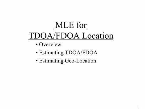
<strong>ML</strong>E <strong>for</strong><br />
<strong>TDOA</strong>/<strong>FDOA</strong> Location<br />
•Overview<br />
• Estimating <strong>TDOA</strong>/<strong>FDOA</strong><br />
• Estimating Geo-Location<br />
1
MULTIPLE-PLATFORM LOCATION<br />
s(<br />
t − t1)<br />
e<br />
jω<br />
s(t)<br />
1<br />
t<br />
Data Link<br />
Emitter to be located<br />
s(<br />
t − t2)<br />
e<br />
jω<br />
s(<br />
t − t3)<br />
e<br />
2<br />
t<br />
Data<br />
Link<br />
jω<br />
3<br />
t<br />
2
ν 21 = ω 2 – ω 1<br />
= constant<br />
<strong>FDOA</strong><br />
Frequency-<br />
Difference-<br />
Of-<br />
Arrival<br />
<strong>TDOA</strong>/<strong>FDOA</strong> LOCATION<br />
<strong>TDOA</strong><br />
Time-<br />
Difference-<br />
Of-<br />
Arrival<br />
ν 23 = ω 2 – ω 3<br />
= constant<br />
s(<br />
t − t1)<br />
e<br />
jω<br />
s(t)<br />
1<br />
t<br />
Data Link<br />
τ 21 = t 2 – t 1<br />
= constant<br />
s(<br />
t − t2)<br />
e<br />
jω<br />
s(<br />
t − t3)<br />
e<br />
2<br />
t<br />
Data<br />
Link<br />
jω<br />
3<br />
t<br />
τ 23 = t 2 –t 3<br />
= constant<br />
3
Estimating <strong>TDOA</strong>/<strong>FDOA</strong><br />
4
SIGNAL MODEL<br />
Will Process Equivalent Lowpass signal, BW = B Hz<br />
– Representing RF signal with RF BW = B Hz<br />
Sampled at Fs > B complex samples/sec<br />
Collection Time T sec<br />
At each receiver:<br />
BPF ADC<br />
cos(ω 1 t)<br />
Make<br />
LPE<br />
Signal<br />
Equalize<br />
-B/2<br />
X RF (f)<br />
X(f)<br />
X f LPE(f)<br />
B/2<br />
f<br />
f<br />
f<br />
5
DOPPLER & DELAY MODEL<br />
s(t) sr (t) = s(t – τ(t))<br />
Tx Rx<br />
R(t)<br />
Propagation Time: τ(t) = R(t)/c<br />
R o<br />
( t)<br />
= R + vt + ( a / 2)<br />
t<br />
2<br />
+ !<br />
Use linear approximation – assumes small<br />
change in velocity over observation interval<br />
For Real BP Signals:<br />
sr o<br />
o<br />
( t)<br />
= s(<br />
t −[<br />
R + vt]<br />
/ c)<br />
= s([<br />
1−<br />
v / c]<br />
t − R / c)<br />
Time<br />
Scaling<br />
Time Delay: τ d<br />
6
~ s<br />
r<br />
DOPPLER & DELAY MODEL (continued)<br />
( t)<br />
=<br />
=<br />
~ s ([ 1<br />
Analytic Signals Model<br />
~ j[ ωct<br />
+ φ(<br />
t)]<br />
s ( t)<br />
=<br />
− v/<br />
c]<br />
t<br />
E(<br />
t)<br />
e<br />
−<br />
E([<br />
1−<br />
v/<br />
c]<br />
t −<br />
τ<br />
τ<br />
Now what? Notice that v
~ s<br />
r<br />
DOPPLER & DELAY MODEL (continued)<br />
( t)<br />
=<br />
=<br />
E(<br />
t<br />
e<br />
Narrowband Analytic Signal Model<br />
− jω<br />
−<br />
c<br />
τ<br />
d<br />
τ<br />
Constant<br />
Phase<br />
Term<br />
α= –ω cτ d<br />
e<br />
d<br />
) e<br />
− jω<br />
c<br />
j{<br />
ω<br />
c<br />
t −ω<br />
( v / c)<br />
t<br />
Doppler<br />
Shift<br />
Term<br />
ω d= ω cv/c<br />
e<br />
c<br />
( v / c)<br />
t −ω<br />
jω<br />
c<br />
t<br />
Carrier<br />
Term<br />
E(<br />
t<br />
c<br />
τ<br />
−<br />
d<br />
+ φ(<br />
t −τ<br />
τ<br />
d<br />
) e<br />
d<br />
)}<br />
jφ(<br />
t −τ<br />
Transmitted Signal’s<br />
LPE Signal<br />
Time-Shifted by τ d<br />
Narrowband Lowpass Equivalent Signal Model<br />
jα<br />
sˆ ( t)<br />
= e e d sˆ<br />
( t − τd<br />
r<br />
− jω<br />
This is the signal that actually gets processed digitally<br />
t<br />
)<br />
d<br />
)<br />
8
CRLB <strong>for</strong> <strong>TDOA</strong><br />
We already showed that the CRLB <strong>for</strong> the active sensor case is:<br />
1<br />
C(<br />
<strong>TDOA</strong>)<br />
=<br />
2<br />
8π<br />
N × SNR × B<br />
But here we need to estimate the delay between two noisy<br />
signals rather than between a noisy one and a clean one.<br />
The only difference in the result is: replace SNR by an<br />
effective SNR given by<br />
SNR eff<br />
=<br />
1<br />
SNR<br />
1<br />
1<br />
1 1<br />
+ +<br />
SNR SNR SNR<br />
2<br />
2<br />
rms<br />
where B rms is an effective bandwidth<br />
of the signal computed from the<br />
DFT values S[k].<br />
1<br />
2<br />
B<br />
2<br />
rms<br />
=<br />
1<br />
N<br />
N / 2−1<br />
≈ min{ SNR , SNR<br />
1<br />
∑<br />
k = −N<br />
/ 2<br />
N / 2−1<br />
∑<br />
k<br />
k=<br />
−N<br />
/ 2<br />
2<br />
2<br />
S[<br />
n]<br />
}<br />
S[<br />
k]<br />
2<br />
2<br />
9
CRLB <strong>for</strong> <strong>TDOA</strong> (cont.)<br />
A more familiar <strong>for</strong>m <strong>for</strong> this is in terms of the C-T version of<br />
the problem:<br />
σ<br />
<strong>TDOA</strong><br />
≥<br />
2π<br />
2<br />
B<br />
rms<br />
1<br />
BT × SNR<br />
eff<br />
“seconds”<br />
2<br />
Brms =<br />
∫ f<br />
∫<br />
2<br />
S(<br />
f )<br />
S(<br />
f )<br />
BT = Time-Bandwidth Product (≈ N, number of samples in DT)<br />
B = Noise Bandwidth of Receiver (Hz)<br />
T = Collection Time (sec)<br />
BT is called “Coherent Processing Gain”<br />
(Same effect as the DFT Processing Gain on a sinusoid)<br />
For a signal with rectangular spectrum of RF width of Bs , then the<br />
bound becomes:<br />
0.<br />
55<br />
σ<br />
<strong>TDOA</strong><br />
≥ 2<br />
B<br />
s<br />
BT × SNR<br />
S. Stein, “Algorithms <strong>for</strong> Ambiguity Function Processing,”<br />
IEEE Trans. on ASSP, June 1981<br />
eff<br />
2<br />
2<br />
df<br />
df<br />
10
CRLB <strong>for</strong> <strong>FDOA</strong><br />
Here we take advantage of the time-frequency duality if the FT:<br />
1<br />
C(<br />
<strong>FDOA</strong>)<br />
=<br />
2<br />
8π<br />
N × SNR<br />
2<br />
eff × Trms<br />
where T rms is an effective duration<br />
of the signal computed from the<br />
signal samples s[k].<br />
Again… we use the same effective SNR:<br />
SNR eff<br />
=<br />
1<br />
SNR<br />
1<br />
1<br />
1 1<br />
+ +<br />
SNR SNR SNR<br />
2<br />
1<br />
2<br />
T<br />
2<br />
rms<br />
=<br />
1<br />
N<br />
N<br />
/ 2−1<br />
∑<br />
n=<br />
−N<br />
/ 2<br />
N / 2−1<br />
∑<br />
k<br />
n=<br />
−N<br />
/ 2<br />
≈ min{ SNR , SNR<br />
1<br />
2<br />
s[<br />
n]<br />
s[<br />
n]<br />
2<br />
}<br />
2<br />
2<br />
11
CRLB <strong>for</strong> <strong>FDOA</strong> (cont.)<br />
A more familiar <strong>for</strong>m <strong>for</strong> this is in terms of the C-T version of<br />
the problem:<br />
σ<br />
<strong>FDOA</strong><br />
≥<br />
2π<br />
2<br />
T<br />
rms<br />
1<br />
BT × SNR<br />
eff<br />
“Hz”<br />
2<br />
Trms For a signal with constant envelope of duration T s , then the bound<br />
becomes:<br />
σ<br />
<strong>FDOA</strong><br />
≥ 2<br />
T<br />
s<br />
0.<br />
55<br />
BT × SNR<br />
S. Stein, “Algorithms <strong>for</strong> Ambiguity<br />
Function Processing,” IEEE Trans. on<br />
ASSP, June 1981<br />
eff<br />
=<br />
∫ t<br />
∫<br />
2<br />
s(<br />
t)<br />
s(<br />
t)<br />
2<br />
2<br />
dt<br />
dt<br />
12
Interpreting CRLBs <strong>for</strong> <strong>TDOA</strong>/<strong>FDOA</strong><br />
A more familiar <strong>for</strong>m <strong>for</strong> this is in terms of the C-T version of<br />
the problem:<br />
σ<br />
<strong>TDOA</strong><br />
≥<br />
2π<br />
2<br />
B<br />
rms<br />
1<br />
BT × SNR<br />
eff<br />
σ<br />
<strong>FDOA</strong><br />
≥<br />
2π<br />
• BT pulls the signal up out of the noise<br />
•Large B rms improves <strong>TDOA</strong> accuracy<br />
•Large T rms improves <strong>FDOA</strong> accuracy<br />
Two Examples of Accuracy Bounds:<br />
SNR 1 SNR 2 T = T s B = B s σ <strong>TDOA</strong> σ <strong>FDOA</strong><br />
3 dB 30 dB 1 ms 1 MHz 17.4 ns 17.4 Hz<br />
3 dB 30 dB 100 ms 10 kHz 1.7 µs 0.17 Hz<br />
2<br />
T<br />
rms<br />
1<br />
BT × SNR<br />
eff<br />
13
<strong>ML</strong>E <strong>for</strong> <strong>TDOA</strong>/<strong>FDOA</strong><br />
S. Stein, “Differential Delay/Doppler <strong>ML</strong><br />
Estimation with Unknown Signals,” IEEE<br />
Trans. on SP, August 1993<br />
We already showed that the <strong>ML</strong> Estimate of delay <strong>for</strong> the<br />
active sensor case is the Cross-Correlation of the time signals.<br />
T<br />
∫<br />
C(<br />
τ ) = s ( t)<br />
s ( t + τ )<br />
0<br />
1<br />
2<br />
By the time-frequency duality the <strong>ML</strong> estimate <strong>for</strong> doppler<br />
shift should be Cross-Correlation of the FT, which is<br />
mathematically equivalent to<br />
C(<br />
ω)<br />
=<br />
A(<br />
ω,<br />
τ ) =<br />
T<br />
∫<br />
0<br />
T<br />
∫<br />
0<br />
s<br />
s<br />
1<br />
1<br />
( t)<br />
s<br />
( t)<br />
s<br />
2<br />
2<br />
( t)<br />
e<br />
− jωt<br />
( t + τ ) e<br />
dt<br />
dt<br />
− jωt<br />
dt<br />
Find Peak of |C(τ)|<br />
Find Peak of |C(ω)|<br />
The <strong>ML</strong> estimate of the <strong>TDOA</strong>/<strong>FDOA</strong> has been shown to be:<br />
Find Peak of |A(ω,τ)|<br />
14
LPE Rx<br />
Signals<br />
At Two<br />
Receivers<br />
<strong>ML</strong> <strong>Estimator</strong> <strong>for</strong> <strong>TDOA</strong>/<strong>FDOA</strong> (cont.)<br />
jα<br />
1( ) t s<br />
2( ) t s<br />
jω<br />
t<br />
= e e d s ( t −τ<br />
1 d<br />
Delay<br />
τ<br />
Called:<br />
• Ambiguity Function<br />
• Complex Ambiguity Function (CAF)<br />
• Cross-Correlation Surface<br />
)<br />
Doppler<br />
ω<br />
ω<br />
ωd “Compare”<br />
Signals<br />
For all<br />
Delays &<br />
Dopplers<br />
Ambiguity Function<br />
τ<br />
Find<br />
Peak<br />
of<br />
|A(ω,τ)|<br />
τ d<br />
15
<strong>ML</strong> <strong>Estimator</strong> <strong>for</strong> <strong>TDOA</strong>/<strong>FDOA</strong> (cont.)<br />
How well do we expect the Cross-Correlation Processing to<br />
per<strong>for</strong>m?<br />
Well… it is the <strong>ML</strong> estimator so it is not necessarily optimum.<br />
But… we know that an <strong>ML</strong> estimate is asymptotically<br />
• Unbiased & Efficient (that means it achieves the CRLB)<br />
• Gaussian<br />
ˆ<br />
−1<br />
θ<strong>ML</strong><br />
~ N ( θ,<br />
I ( θ))<br />
Those are some VERY nice properties that we can make use of<br />
in our location accuracy analysis!!!<br />
16
Properties of the CAF<br />
• Consider when τ = τ T<br />
d [ ] 2<br />
∫<br />
jω<br />
t<br />
A(<br />
ω,<br />
τd<br />
) = s(<br />
t)<br />
e<br />
|A(ω,τ d )|<br />
ω d<br />
width ∼ 1/T<br />
• Consider when ω = ω d<br />
|A(ω d ,τ)|<br />
τ d<br />
width ∼ 1/BW<br />
ω<br />
τ<br />
A(<br />
ω<br />
d<br />
0<br />
d<br />
e<br />
− jωt<br />
dt<br />
like windowed FT of sinusoid<br />
where window is |s(t)| 2<br />
, τ)<br />
=<br />
T<br />
∫<br />
0<br />
s(<br />
t)<br />
s(<br />
t<br />
−<br />
τ<br />
d<br />
correlation<br />
+ τ)<br />
dt<br />
17
<strong>TDOA</strong> ACCURACY REVISITED<br />
<strong>TDOA</strong> Accuracy depends on:<br />
» Effective SNR: SNR eff<br />
» RMS Widths: B rms = RMS Bandwidth<br />
XCorr<br />
Function<br />
XCorr<br />
Function<br />
~1/B rms<br />
Narrow B rms Case<br />
Poor Accuracy<br />
<strong>TDOA</strong><br />
Wide B rms Case<br />
Good Accuracy<br />
<strong>TDOA</strong><br />
2<br />
Brms =<br />
∫<br />
f<br />
∫<br />
2<br />
S(<br />
f )<br />
S(<br />
f )<br />
2<br />
2<br />
df<br />
df<br />
Low Effective SNR<br />
Causes Spurious Peaks<br />
On Xcorr Function<br />
Narrow Xcorr Function<br />
Less Susceptible to<br />
Spurious Peaks<br />
18
<strong>FDOA</strong> ACCURACY REVISITED<br />
<strong>FDOA</strong> Accuracy depends on:<br />
» Effective SNR: SNR eff<br />
» RMS Widths: D rms = RMS Duration<br />
XCorr<br />
Function<br />
XCorr<br />
Function<br />
~1/D rms<br />
Narrow D rms Case<br />
Poor Accuracy<br />
<strong>FDOA</strong><br />
Wide D rms Case<br />
Good Accuracy<br />
<strong>FDOA</strong><br />
2<br />
Brms =<br />
∫<br />
f<br />
∫<br />
2<br />
S(<br />
f )<br />
S(<br />
f )<br />
2<br />
2<br />
df<br />
df<br />
Low Effective SNR<br />
Causes Spurious Peaks<br />
On Xcorr Function<br />
Narrow Xcorr Function<br />
Less Susceptible to<br />
Spurious Peaks<br />
19
COMPUTING THE AMBIGUITY FUNCTION<br />
Direct computation based on the equation <strong>for</strong> the ambiguity<br />
function leads to computationally inefficient methods.<br />
In EECE 521 notes we showed how to use decimation to<br />
efficiently compute the ambiguity function<br />
20
Estimating Geo-Location<br />
21
<strong>TDOA</strong>/<strong>FDOA</strong> LOCATION<br />
Data Link<br />
Data<br />
Link<br />
Centralized Network of P<br />
•“P-Choose-2” Pairs<br />
“P-Choose-2” <strong>TDOA</strong> Measurements<br />
“P-Choose-2” <strong>FDOA</strong> Measurements<br />
• Warning: Watch out <strong>for</strong> Correlation<br />
Effect Due to Signal-Data-In-Common<br />
Data<br />
Link<br />
22
<strong>TDOA</strong>/<strong>FDOA</strong> LOCATION<br />
Pair-Wise Network of P<br />
• P/2 Pairs<br />
P/2 <strong>TDOA</strong> Measurements<br />
P/2 <strong>FDOA</strong> Measurements<br />
• Many ways to select P/2 pairs<br />
• Warning: Not all pairings are equally<br />
good!!! The Dashed Pairs are Better<br />
23
<strong>TDOA</strong>/<strong>FDOA</strong> Measurement Model<br />
Given N <strong>TDOA</strong>/<strong>FDOA</strong> measurements with corresponding 2×2 Cov. Matrices<br />
( ˆ τ1, ˆ ν1),<br />
( ˆ τ 2,<br />
ˆ ν 2 ), … , ( ˆ τ N , ˆ ν N ) Assume pair-wise network, so…<br />
C C , … , C<br />
<strong>TDOA</strong>/<strong>FDOA</strong> pairs are uncorrelated<br />
For notational purposes… define the 2N measurements r(n) n = 1, 2, …, 2N<br />
r<br />
2n−1<br />
r<br />
2n<br />
= ˆ τ<br />
= ˆ ν<br />
n<br />
n<br />
,<br />
,<br />
1,<br />
2<br />
n<br />
n<br />
=<br />
=<br />
1,<br />
2,<br />
1,<br />
2,<br />
…,<br />
…,<br />
N<br />
N<br />
N<br />
r<br />
=<br />
[ 1 r2<br />
! r2<br />
N<br />
r ]<br />
Data Vector<br />
Now, those are the <strong>TDOA</strong>/<strong>FDOA</strong> estimates… so the true values are notated as:<br />
s<br />
2n−1<br />
s<br />
2n<br />
= τ<br />
= ν<br />
n<br />
n<br />
,<br />
,<br />
n<br />
n<br />
( τ1, ν1),<br />
( τ 2,<br />
ν 2 ), … , ( τ N , ν N<br />
=<br />
=<br />
1,<br />
2,<br />
1,<br />
2,<br />
…,<br />
…,<br />
N<br />
N<br />
)<br />
s<br />
=<br />
[ 1 s2<br />
! s2N<br />
s ]<br />
“Signal” Vector<br />
T<br />
T<br />
24
<strong>TDOA</strong>/<strong>FDOA</strong> Measurement Model (cont.)<br />
Each of these measurements r(n) has an error ε(n) associated with it, so…<br />
r = s +<br />
Because these measurements were estimated using an <strong>ML</strong> estimator (with<br />
sufficiently large number of signal samples) we know that error vector ε is a<br />
zero-mean Gaussian vector with cov. matrix C given by:<br />
⎡C1<br />
0 0 ⎤<br />
⎢<br />
⎥<br />
C = diag{ C1<br />
, C2,<br />
… , CN<br />
} = ⎢ 0 # 0 ⎥<br />
⎢<br />
⎥<br />
⎢<br />
⎣ 0 0 CN<br />
⎥<br />
⎦<br />
The true <strong>TDOA</strong>/<strong>FDOA</strong> values depend on:<br />
Emitter Parms: (xe , ye , ze ) and transmit frequency fe xe = [ xe ye ze fe ] T<br />
Assumes that<br />
<strong>TDOA</strong>/<strong>FDOA</strong><br />
pairs are<br />
uncorrelated!!!<br />
Receivers’ Nav Data (positions & velocities): The totality of it called xr r = s(<br />
xe<br />
; xr<br />
) +<br />
ε<br />
ε<br />
• Deterministic “Signal” + Gaussian Noise<br />
• “Signal” is nonlinearly related to parms<br />
To complete the model… we need to know how s(x e;x r) depends on x e and x r.<br />
Thus we need to find <strong>TDOA</strong> & <strong>FDOA</strong> as functions of x e and x r<br />
25
<strong>TDOA</strong>/<strong>FDOA</strong> Measurement Model (cont.)<br />
Here we’ll simplify to the x-y plane… extension is straight-<strong>for</strong>ward.<br />
Two Receivers with: (x 1, y 1, Vx 1, Vy 1) and (x 2, y 2, Vx 2, Vy 2)<br />
Emitter with: (x e, y e)<br />
(Let R i be the range between Receiver i and the emitter; c is the speed of light.)<br />
The <strong>TDOA</strong> and <strong>FDOA</strong> are given by:<br />
s ( x , y ) = τ<br />
1<br />
e<br />
e<br />
=<br />
=<br />
s ( x , y , f ) = ν<br />
2<br />
e<br />
e<br />
e<br />
1<br />
c<br />
12<br />
f<br />
c<br />
e<br />
12<br />
⎛<br />
⎜<br />
⎝<br />
=<br />
⎡<br />
⎢<br />
⎢<br />
⎢⎣<br />
=<br />
R<br />
1<br />
− R<br />
c<br />
2<br />
2<br />
2<br />
2<br />
2<br />
( x1<br />
− xe<br />
) + ( y1<br />
− ye<br />
) − ( x2<br />
− xe<br />
) + ( y2<br />
− ye<br />
) ⎟<br />
⎠<br />
f<br />
c<br />
e<br />
d<br />
dt<br />
( R − R )<br />
( x1<br />
− xe<br />
) Vx1<br />
+ ( y1<br />
− ye<br />
)<br />
( x − x<br />
2 ) + ( y − y )<br />
1<br />
1<br />
e<br />
2<br />
1<br />
e<br />
Vy<br />
1<br />
2<br />
−<br />
( ) ( )<br />
( ) ( ) ⎥ ⎥⎥<br />
x2<br />
− xe<br />
Vx2<br />
+ y2<br />
− ye<br />
Vy2<br />
2<br />
2<br />
x − x + y − y<br />
2<br />
e<br />
2<br />
⎞<br />
e<br />
⎤<br />
⎦<br />
26
CRLB <strong>for</strong> Geo-Location via <strong>TDOA</strong>/<strong>FDOA</strong><br />
Recall: For the General Gaussian Data case the CRLB depends on a FIM that<br />
has structure like this:<br />
[ J(<br />
θ)<br />
]<br />
nm<br />
T<br />
⎡∂µ<br />
x ( θ)<br />
⎤ −1<br />
⎡∂µ<br />
x ( θ)<br />
⎤<br />
= ⎢ ⎥ Cx<br />
( θ)<br />
⎢ ⎥<br />
⎣ ∂θn<br />
'$<br />
$ $ ⎦$<br />
$ &$<br />
$ ⎣ ∂θm<br />
$ $ $ % ⎦<br />
variability<br />
of mean w.r.t. parms<br />
+<br />
1 ⎡<br />
1 ( ) 1 ( ) ⎤<br />
− ∂Cx<br />
θ − ∂Cx<br />
θ<br />
tr⎢Cx<br />
( θ)<br />
Cx<br />
( θ)<br />
⎥<br />
2 ⎢<br />
⎥<br />
'$<br />
⎣<br />
∂θn<br />
∂θm<br />
$ $ $ $ $ &$<br />
$ $ $ $ $ $ % ⎦<br />
variability<br />
of cov. w.r.t. parms<br />
Here we have a deterministic “signal” plus Gaussian noise so we only have the<br />
1 st term… Using the notation introduced here gives…<br />
C<br />
CRLB<br />
( x<br />
e<br />
)<br />
⎡ T<br />
∂s<br />
( x<br />
= ⎢<br />
⎢⎣<br />
∂xe<br />
H T<br />
e<br />
)<br />
C<br />
−1<br />
∂s(<br />
x<br />
∂x<br />
e<br />
e<br />
) ⎤<br />
⎥<br />
⎥⎦<br />
−1<br />
Called the “Jacobian” … <strong>for</strong> the 3-D location with<br />
<strong>TDOA</strong>/<strong>FDOA</strong> will be a 2N × 4 matrix whose columns<br />
are derivatives of s w.r.t. each of the 4 parameters.<br />
H<br />
()<br />
27
CRLB <strong>for</strong> Geo-Loc. via <strong>TDOA</strong>/<strong>FDOA</strong> (cont.)<br />
<strong>TDOA</strong>/<strong>FDOA</strong> Jacobian:<br />
H<br />
= ∆<br />
∂s(<br />
x<br />
∂x<br />
e<br />
e<br />
)<br />
⎡ ∂s1(<br />
xe<br />
)<br />
⎢<br />
∂x<br />
⎢ e<br />
⎢ ∂s2<br />
( xe<br />
)<br />
= ⎢ ∂xe<br />
⎢<br />
(<br />
⎢<br />
⎢∂s2<br />
N ( xe<br />
)<br />
⎢<br />
⎣ ∂xe<br />
∂<br />
∂xe<br />
∂s1(<br />
xe<br />
)<br />
∂ye<br />
∂s2<br />
( xe<br />
)<br />
∂ye<br />
(<br />
∂s2N<br />
( xe<br />
)<br />
∂y<br />
e<br />
∂<br />
∂ye<br />
∂s1(<br />
xe<br />
)<br />
∂ze<br />
∂s2<br />
( xe<br />
)<br />
∂ze<br />
(<br />
∂s2N<br />
( xe<br />
)<br />
∂z<br />
e<br />
∂<br />
∂ze<br />
∂s1(<br />
xe<br />
) ⎤<br />
∂f<br />
⎥<br />
e ⎥<br />
∂s2<br />
( xe<br />
) ⎥<br />
∂f<br />
⎥<br />
e<br />
(<br />
⎥<br />
⎥<br />
∂s2N<br />
( xe<br />
) ⎥<br />
∂f<br />
⎥<br />
e ⎦<br />
Jacobian can be computed <strong>for</strong> any desired Rx-Emitter Scenario<br />
Then… plug it into () to compute the CRLB <strong>for</strong> that scenario:<br />
C<br />
CRLB<br />
( x<br />
e<br />
)<br />
[ ] 1<br />
T −1<br />
−<br />
H C<br />
= H<br />
∂<br />
∂fe<br />
28
CRLB Studies<br />
The Location CRLB can be used to study various aspects of the emitter location<br />
problem. It can be used to study the effect of<br />
• Rx-Emitter Geometry and/or Plat<strong>for</strong>m Velocity<br />
• <strong>TDOA</strong> accuracy vs. <strong>FDOA</strong> accuracy<br />
• Number of Plat<strong>for</strong>ms<br />
• Plat<strong>for</strong>m Pairings<br />
• Etc., Etc., Etc…<br />
Once you have computed the CRLB Covariance C CRLB you can use it to<br />
compute and plot error ellipsoids.<br />
Assumes Geo-Location Error<br />
is Gaussian…<br />
Usually reasonably valid<br />
Emitter<br />
Sensor 1<br />
k 1 σ <strong>TDOA</strong><br />
V V<br />
Faster than doing Monte<br />
Carlo Simulation Runs!!!<br />
Sensor 2<br />
k 2 σ <strong>FDOA</strong><br />
29
CRLB Studies (cont.)<br />
Error Ellipsoids: If our C CRLB is 4×4… how do we get 2-D ellipses to plot???<br />
Projections!<br />
z<br />
Projections of 3-D Ellipsoids onto 2-D Space<br />
y<br />
x<br />
2-D Projections Show<br />
Expected Variation<br />
in 2-D Space<br />
30
CRLB Studies (cont.)<br />
Another useful thing that can be computed from the CRLB is the CEP <strong>for</strong> the<br />
location problem. For the 2-D case:<br />
within 10%<br />
1<br />
2<br />
2<br />
1<br />
CEP ≈ 0.<br />
75 λ + λ = 0.<br />
75 σ + σ<br />
Eigen-Values of the<br />
2-D Cov. Matrix<br />
Down Range<br />
2<br />
2<br />
Diagonal elements of<br />
the 2-D Cov. Matrix<br />
CEP = 80<br />
CEP = 40<br />
CEP = 20<br />
CEP = 10<br />
Cross Range<br />
“Circular Error Probable”<br />
= radius of a circle that when<br />
centered at the estimate’s mean,<br />
contains 50% of the estimates<br />
CEP Contour Plots are<br />
Good Ways to Assess<br />
Location Per<strong>for</strong>mance<br />
31
CRLB Studies (cont.)<br />
Sensor<br />
Geometry and <strong>TDOA</strong> vs. <strong>FDOA</strong> Trade-Offs<br />
Both Important <strong>FDOA</strong> Important <strong>TDOA</strong> Important<br />
Target<br />
<strong>TDOA</strong> Only<br />
<strong>FDOA</strong> Only<br />
<strong>TDOA</strong>/<strong>FDOA</strong><br />
Target<br />
<strong>TDOA</strong> Only<br />
Target<br />
<strong>FDOA</strong><br />
Only<br />
25<br />
32
<strong>Estimator</strong> <strong>for</strong> Geo-Location via <strong>TDOA</strong>/<strong>FDOA</strong><br />
Because we have used the <strong>ML</strong> estimator to get the <strong>TDOA</strong>/<strong>FDOA</strong><br />
estimates the <strong>ML</strong>’s asymptotic properties tell us that we have<br />
Gaussian <strong>TDOA</strong>/<strong>FDOA</strong> measurements<br />
Because the <strong>TDOA</strong>/<strong>FDOA</strong> measurement model is nonlinear it is<br />
unlikely that we can find a truly optimal estimate… so we again<br />
resort to the <strong>ML</strong>. For the <strong>ML</strong> of a Nonlinear Signal in Gaussian we<br />
generally have to proceed numerically.<br />
One way to do Numerical <strong>ML</strong>E is <strong>ML</strong> Newton-Raphson (need vector<br />
version):<br />
θˆ<br />
k+<br />
1<br />
= θˆ<br />
k<br />
⎧<br />
⎪⎡∂<br />
− ⎨⎢<br />
⎪⎢<br />
⎩⎣<br />
2<br />
Hessian: p×p matrix<br />
ln p(<br />
x;<br />
θ)<br />
⎤<br />
T ⎥<br />
∂θ∂θ<br />
⎥⎦<br />
−1<br />
⎫<br />
∂ln<br />
p(<br />
x;<br />
θ)<br />
⎪<br />
⎬<br />
∂θ<br />
⎪<br />
⎭<br />
However, the “Hessian” requires a second derivative…<br />
This can add complexity in practice… Alternative:<br />
Gauss-Newton Nonlinear Least Squares based on linearizing the model.<br />
θ=<br />
θˆ<br />
k<br />
Gradient: p×1 vector<br />
33