Lab 7: Amplitude Modulation with Suppressed Carrier

ECEN 4652/5002 Communications Lab Spring 2013
3-06-13 P. Mathys
Lab 7: Amplitude Modulation with Suppressed Carrier
1 Introduction
Many channels either cannot be used to transmit baseband signals at all, or pass signal
energy very inefficiently, except for a relatively narrow passband region at frequencies substantially
higher than those contained in a baseband message signal. A well-known example
is electromagnetic transmission of radio signals at a frequency fc in free space which requires
an antenna of length comparable to λc/2 for a dipole, or λc/4 for a monopole, where
λc = 3×10 8 /fc is the wavelength in meters corresponding to fc in Hz. Thus, transmission at
fc = 10 kHz would require an antenna of length comparable to 15 km for a dipole, whereas
at fc = 900 MHz a length of 8.3 cm is enough for the monopole antenna of a cell phone.
1.1 Amplitude Modulation with Suppressed Carrier
The most straightforward way to shift a signal spectrum from baseband to a passband
location with center frequency fc is to make use of the frequency shift property of the
Fourier transform (FT) which says that
m(t) e j(2πfct+θc)
⇐⇒ M(f − fc) e jθc .
Thus, Ac m(t) e j(2πfct+θc) is a complex-valued bandpass signal with amplitude Ac and center
frequency fc if m(t) is a (bandlimited) baseband signal. To make this into a real bandpass
signal x(t), write
x(t) = Re{Ac m(t) e j(2πfct+θc) } = Re Ac m(t) cos(2πfct + θc) + j sin(2πfct + θc)
= Ac m(t) cos(2πfct + θc) ,
where for the last equality it is assumed that m(t) is real-valued. The signal x(t) obtained in
this way is a AM-DSB-SC (amplitude modulation, double side-band, suppressed carrier)
signal with carrier frequency fc, carrier phase θc and Fourier transform
x(t) = Ac m(t) cos(2πfct + θc) ⇐⇒ X(f) = Ac
M(f − fc) e
2
jθc + M(f + fc) e −jθc .
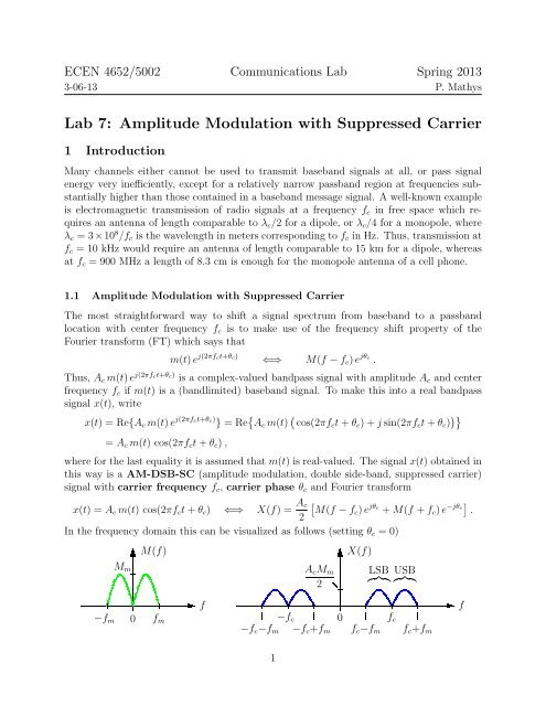
In the frequency domain this can be visualized as follows (setting θc = 0)
Mm
M(f)
−fm 0 fm
f
AcMm
2
−fc
−fc−fm −fc+fm
1
0
X(f)
fc−fm
LSB
USB
fc
fc+fm
f

From the figure it is evident that if the bandwidth of m(t) is fm, then the bandwidth of x(t)
is 2fm, which explains the “DSB” in AM-DSB-SC. It is also clear that if m(t) has no dc
component (which is the case for speech and music signals, for instance), then x(t) has no
component at the carrier frequency fc, which is where the “SC” comes from. The portion
of the spectrum of x(t) for which fc − fm ≤ |f| < fc is called the lower side-band (LSB),
whereas the portion for which fc < |f| ≤ fc + fm is called the upper side-band (USB).
To recover m(t) undistorted from x(t), fc ≥ fm is required, but usually fc ≫ fm in practice.
The block diagram of an AM-DSB-SC transmission system is shown in the following figure.
Transmitter
mw(t) LPF m(t) x(t) Channel
r(t) v(t) LPF ˆm(t)
× + ×
at fm
HC(f)
at fL
Ac cos(2πfct + θc)
Carrier Oscillator
Noise n(t)
Channel Model
Receiver
2cos(2πfct + θc)
Local Oscillator
The transmitter consists of a LPF that bandlimits the wideband message signal mw(t) to
|f| ≤ fm and the modulator which multiplies the resulting message signal m(t) with the
output Ac cos(2πfct + θc) of the carrier oscillator. The channel is modeled as a filter HC(f)
with noise added at the output. In the receiver the incoming signal r(t) is multiplied by
the local oscillator signal cos(2πfct + θc) and then lowpass filtered at fL. Assuming an ideal
channel with attenuation γ and no noise such that r(t) = γ x(t), the demodulation operation
can be described as
v(t) = 2r(t) cos(2πfct+θc) = 2γAcm(t) cos 2 (2πfct+θc) = γAcm(t) 1 + cos(4πfct+2θc) .
Assuming that fc ≥ fm, the second term, which is a AM-DSB-SC signal with carrier frequency
2fc and carrier phase 2θc, can be removed by lowpass filtering at fL = fm and
thus
ˆm(t) = γAc m(t) .
In the absence of noise and other channel impairments this is an exact replica of the transmitted
message signal, scaled by γAc.
If m(t) is a wide-sense stationary process with mean E[m] and autocorrelation function
Rm(τ), then the autocorrelation function of the AM-DSB-SC signal x(t) can be computed
as
Rx(t1, t2) = E Ac m(t1) cos(2πfct1 + θc) A ∗ c m ∗ (t2) cos(2πfct2 + θc)
= |Ac| 2 E[m(t1) m ∗ (t2)]
= Rm(t1 − t2)
= |Ac| 2
cos(2πfct1 + θc) cos(2πfct2 + θc)
cos 2πfc(t1 − t2) + cos
2πfc(t1 + t2) + 2θc
= 1
2
2 Rm(t1 − t2) cos 2πfc(t1 − t2) + cos
2πfc(t1 + t2) + 2θc .
2

Note that x(t) is a cyclostationary process with period 1/fc. The time-averaged autocorrelation
function of x(t) is
¯Rx(τ) = fc
1/fc
0
Rx(t + τ, t) dt =
|Ac| 2
2 Rm(τ) cos(2πfcτ) .
Thus, if m(t) has PSD Sm(f), then the PSD of the AM-DSB-SC signal x(t) is
Sx(f) =
2 |Ac|
Sm(f − fc) + Sm(f + fc)
4
.
The PSD of a speech signal after AM-DSB-SC modulation with fc = 8000 Hz and fm = 4000
Hz is shown in the following graph.
10log 10 (S x (f)) [dB]
0
−10
−20
−30
−40
−50
PSD, P x =0.0072139, P x (f 1 ,f 2 ) = 49.9999%, F s =44100 Hz, N=44100, NN=3, Δ f =1 Hz
−60
0 2000 4000 6000 8000
f [Hz]
10000 12000 14000 16000
1.2 Coherent AM Reception
An idealizing assumption which is tacitly made in the AM-DSB-SC transmission system
block diagram given earlier, is that the local oscillator at the receiver is synchronized with
the carrier oscillator at the transmitter. To see why this synchronism between transmitter
and receiver is important, assume that the local oscillator signal is 2 cos(2πfct), but the
received AM-DSB-SC signal is r(t) = γAcm(t) cos(2πfct + θe), i.e., there is a phase error θe
between transmitter and receiver. Now the receiver computes
and thus
v(t) = 2γAc m(t) cos(2πfct + θe) cos(2πfct) = γAc m(t) cos θe + cos(4πfct + θe) ,
ˆm(t) = γAc cos θe m(t) ,
after the LPF at fL = fm. A small phase error |θe| ≪ π/2 therefore attenuates m(t) by
cos(θe) ≈ 1, which presents no big problem, but phase errors close to ±90 ◦ attenuate m(t)
substantially or even suppress it altogether. This is especially annoying when θe varies with
time and ˆm(t) changes periodically in intensity. On the positive side, however, this means
that two AM-DSB-SC signals, such as
xi(t) = Acmi(t) cos(2πfct) , and xq(t) = Acmq(t) cos(2πfct + π/2) ,
3

can use the same carrier frequency fc to transmit two independent message signals mi(t)
and mq(t). This is known as quadrature amplitude modulation (QAM), and xi(t)
is called the in-phase component of the AM signal at fc, whereas xq(t) is called the
quadrature component. At any rate, it is crucial for the correct demodulation of AM
signals with suppressed carrier, that the receiver is phase (and frequency) synchronized
with the transmitter. Receivers of this type are called synchronous or coherent receivers.
In practice the maintenance of exact phase synchronism between two oscillators in different
physical locations is quite a non-trivial problem and requires a considerable amount of active
hardware and/or software.
1.3 AM-SSB-SC and AM-VSB-SC
One of the disadvantages of AM-DSB-SC is that it occupies twice the bandwidth of the
original message signal. One straightforward way to reduce the bandwidth to the original
value is to only keep one of the sidebands of the AM signal and suppress the other one. The
resulting AM signals are known as AM-SSB-LSB (amplitude modulation, single sideband,
lower sideband) and as AM-SSB-USB (amplitude modulation, single sideband, upper sideband)
depending on whether the lower or upper sideband is kept. To convert AM-DSB-SC
to AM-SSB-SC (either LSB or USB), the AM-DSB-SC signal can be filtered with a bandpass
filter (BPF) as shown in the following block diagram.
mw(t) LPF m(t) x(t) BPF xB(t)
×
at fm
HBx(f)
Ac cos(2πfct + θc)
Carrier Oscillator
For AM-SSB-USB, for example, the transmitter filter HBx(f) is chosen as shown in the
following figure.
Filter for AM-SSB-USB
1
HBx(f)
−fc−fm −fc −fc+fm 0 fc−fm fc fc+fm
A problem with this filter are the sharp cutoffs needed near fc, especially if m(t) has a dc
component (which is the case for analog TV broadcast signals, for instance). To alleviate
this problem, vestigial sideband (VSB) modulation can be used. This is essentially a
compromise between AM-DSB and AM-SSB, with a well controlled (usually linear) overall
transition from the passband of HB(f) to the stopband near fc, extending over a range of
2∆ around fc. Depending on whether the lower or upper sideband is kept, the resulting
4
f

AM signal is either called AM-VSB-LSB (amplitude modulation, vestigial sideband, lower
sideband) or AM-VSB-USB (amplitude modulation, vestigial sideband, upper sideband).
An example of a filter HB(f) that converts a AM-DSB-SC signal to a AM-VSB-USB-SC
signal is shown in the following figure.
Filter for AM-VSB-USB
−fc−fm −fc −fc+fm
−fc−∆ −fc+∆
1
HB(f)
0 fc−fm fc fc+fm
fc−∆ fc+∆
Demodulation of AM-SSB-SC signals and AM-VSB-SC signals is done in a similar fashion
as for AM-DSB-SC by multiplying the received signal with the local oscillator signal
2 cos(2πfct + θc), followed by lowpass filtering at fm. To remove noise and/or interference
from the unused (portion of the) sideband, a BPF should be used at the input of the receiver,
as shown in the following blockdiagram.
r(t) BPF rB(t) v(t) LPF ˆm(t)
×
HBr(f)
at fL
2cos(2πfct + θc)
Local Oscillator
For AM-SSB-SC the same BPF can be used for both the transmitter and the receiver. For
AM-VSB-SC the product HBx(f)HBr(f) of the frequency responses of the BPFs at the
transmitter and receiver must be equal to HB(f) as shown above.
1.4 Bandpass Filters
Suppose you have a lowpass filter hL(t) ⇔ HL(f), e.g., an LPF with trapezoidal frequency
response and thus
hL(t) = sin(2πfLt)
πt
sin(2παfLt)
2παfLt
⇐⇒
−(1+α)fL
−(1−α)fL
5
1
0
HL(f)
(1−α)fL
(1+α)fL
0 ≤ α ≤ 1
f
f

By making use of the frequency shift property of the FT, this LPF can be converted to a
BPF hBP (t) ⇔ HBP (f) which is symmetric about some center frequency fc ≥ (1 + α) fL
(where α = 0 for an ideal LPF) by
hBP (t) = 2 hL(t) cos(2πfct) ⇐⇒ HBP (f) = HL(f) ∗ [δ(f − fc) + δ(f + fc)] .
BPFs that are obtained from ideal LPFs (i.e., α → 0) are well suited for picking out one
particular signal from several FDM (frequency division multiplexed) signals, or for generating
SSB (single sideband) AM signals from DSB AM signals. BPFs that are obtained from LPFs
with trapezoidal frequency response can be used for similar tasks, but in addition they can
also be used to convert frequency to amplitude (in the transition region of the BPF) and to
generate VSB (vestigial sideband) AM signals.
1.5 Carrier Frequency Extraction
Let r(t) be a received noiseless AM-DSB-SC signal with attenuation γ, i.e.,
r(t) = γ x(t) = γAc m(t) cos
2π(fc + fe)t + θe ,
where fe is the frequency error and θe is the phase error between the transmitter and the
receiver. To obtain (an estimate of) the error signal ψ(t) = 2πfet + θe from r(t), start from
squaring r(t) to obtain
r 2 (t) = γ 2 A 2 c m 2 (t) cos 2 γ
2π(fc + fe)t + θe = 2 A2 c m2 (t)
1 + cos 4π(fc + fe)t + 2θe .
2
Multiplying this by 2 cos(4πfct) yields
vi(t) = γ 2 A 2 c m 2 (t) 1 + cos
4π(fc + fe)t + 2θe cos 4πfct
= A(t) 2 cos 4πfct + cos(4πfet + 2θe) + cos
4π(2fc + fe)t + 2θe ,
where A(t) = γ 2 A 2 c m 2 (t)/2 is a time-varying amplitude. Simlarly, multiplying by -2 sin 4πfct
results in
vq(t) = −γ 2 A 2 c m 2 (t) 1 + cos
4π(fc + fe)t + 2θe sin 4πfct
= A(t) − 2 sin 4πfct + sin(4πfet + 2θe) − sin
4π(2fc + fe)t + 2θe .
Thus, after lowpass filtering with 2fe < fL < fc,
wi(t) = A(t) cos(4πfet + 2θe) and wq(t) = A(t) sin(4πfet + 2θe) .
Finally, the error estimate ψ(t) is obtained by taking an inverse tangent and dividing by 2
as follows
ψ(t) = 1
2 tan−1
wq(t)
.
wi(t)
This whole process is shown in blockdiagram form in the next figure.
6

(t)
(.) 2
r 2 (t)
•
×
2cos4πfct
×
vi(t)
vq(t)
−2sin4πfct
LPF
at fL
LPF
at fL
wi(t)
tan −1 wq(t)
wi(t)
wq(t)
Note that, before the division by 2 to obtain ψ(t), it is crucial that the phase (which is
only resolved modulo 2π by the inverse tangent) is unwrapped. To demodulate the received
AM-DSB-SC signal r(t), the local oscillator term 2 cos(2πfct + ψ(t)) is then used instead of
the 2 cos(2πfct + θc) term shown in an earlier blockdiagram.
2 Lab Experiments
E1. AM-DSB-SC Transmitter/Receiver. (a) Write a Matlab function, called amxmtr10
which performs the tasks of a AM-DSB-SC transmitter, i.e., bandlimits the message signal to
fm (using trapfilt) and then multiplies the result with the output of the carrier oscillator.
The header of amxmtr10 looks as follows:
function x = amxmtr10(t,m,fcparms,fmparms)
%amxmtr10 Amplitude Modulation Transmitter V1.0
% >>>>> x = amxmtr10(t,m,fcparms,fmparms)

Test your transmitter using the message signal
Fs = 44100; %Sampling rate
t = [0:Fs-1]/Fs; %Time axis
m = (cos(2*pi*3000*t)+cos(2*pi*5000*t)); %Message signal
as input. Set fc = 8000 Hz, θc = 0 ◦ , fm = 4000, km ≈ 10 . . . 20, and αm = 0.05. The LPF
at the transmitter should remove the frequency component at 5000 Hz. The 3000 Hz cosine
should be moved to fc ± 3000 Hz so that the PSD looks as shown below.
S x (f)
0.07
0.06
0.05
0.04
0.03
0.02
0.01
PSD, P x =0.2498, P x (f 1 ,f 2 ) = 0.1249, F s =44100 Hz, N=44100, NN=1, Δ f =1 Hz
0
0 2000 4000 6000 8000
f [Hz]
10000 12000 14000 16000
(b) Use the speech signal in speech701.wav and the music signal in music701.wav to
generate AM-DSB-SC signals x1(t) and x2(t), respectively, with fc = 8000 Hz, fm = 4000
Hz, km ≈ 10 . . . 20, and αm = 0.05. Use θc = −90 ◦ for the speech signal and θc = 0 ◦ for
the music signal. Create a third signal x3(t) = (x1(t) + x2(t))/2. Look at the PSDs of
each of the three signals. Does the bandwidth for x3(t), which contains two message signals,
change? Also look at the PSDs of the squared AM signals x 2 1(t), x 2 2(t), and x 2 3(t). Is there
any additional information that you can get from the squared signals? If so, what is this
information and for which of the three signals is it actually present? Save the three signals
for later use.
(c) Write a Matlab function called amrcvr10 that demodulates a received AM-DSB-SC
signal r(t) and produces an estimate ˆm(t) of the transmitted message m(t). Here is the
header for this function
8

function mhat = amrcvr10(t,r,fcparms,fmparms)
%amrcvr10 Amplitude Modulation Receiver, V1.0
% >>>>> mhat = amrcvr10(t,r,fcparms,fmparms)

To test your modified trapfilt function, estimate the parameters of the BPF whose frequency
response is shown below and recreate h(t) ⇔ H(f) with your trapfilt function.
∠X(f) [deg]
|X(f)|
1.4
1.2
1
0.8
0.6
0.4
0.2
200
100
−100
FT Approximation , F s =44100 Hz, N=44100, Δ f =1 Hz
0
0 2000 4000 6000 8000 10000 12000 14000 16000
0
−200
0 2000 4000 6000 8000
f [Hz]
10000 12000 14000 16000
(b) Extend the Matlab functions amxmtr10 and amrcvr10 so that they can also be used
transmit and receive AM-SSB-SC and AM-VSB-SC. Call the new functions amxmtr11 and
amrcvr11. The header of amxmtr11 is:
10

function x = amxmtr11(t,m,fcparms,fmparms,fBparms)
%amxmtr11 Amplitude Modulation Transmitter, V1.1
% >>>>> x = amxmtr11(t,m,fcparms,fmparms,fBparms)

10log 10 (S x (f)) [dB]
0
−10
−20
−30
−40
−50
PSD, P x =0.0026165, P x (f 1 ,f 2 ) = 49.9999%, F s =44100 Hz, N=44100, NN=3, Δ f =1 Hz
−60
0 2000 4000 6000 8000
f [Hz]
10000 12000 14000 16000
The header of the receiver function amrcvr11 is:
function mhat = amrcvr11(t,r,fcparms,fmparms,fBparms)
%amrcvr11 Amplitude Modulation Receiver, V1.1
% >>>>> mhat = amrcvr11(t,r,fcparms,fmparms,fBparms)

signals, and demodulating them with the AM receiver function. Use Fs = 44100 Hz, fm =
4000 Hz, fc = 8000 Hz, θc = 0 ◦ , and, in the case of AM-VSB, ∆ = 1000 Hz. Look at the
PSDs Sx(f) of all four AM signals x(t) and also at the PSDs of x 2 (t). Are they what you
expect them to be? If not, why not?
(d) Analyze and demodulate the signals in the wav-files amsig704.wav and amsig705.wav.
Determine the important parameters such as fc, θc, SSB or VSB, USB or LSB, fm and,
in the case of VSB, ∆. Which parameters can you obtain from PSDs? For which ones do
you actually have to demodulate the received signals? Note that the signals may have noise
and/or interference from other signals added. If this is the case, try to eliminate as much of
the noise/interference as possible. Explain your strategy!
(e) Revisit those AM signals in the files amsig701.wav, amsig702.wav, and amsig703.wav
that you could not demodulate properly in E1(d). Try if using an AM-SSB receiver (which
removes one of the sidebands before demodulation) helps. If so, can you explain why?
E3. Extraction of Carrier Frequency and Phase from AM-DSB-SC Signal. (Experiment
for ECEN 5002, optional for ECEN 4652) (a) Modify your amrcvr11 receiver
function so that it extracts the error estimate ψ(t) = 2πfet + θe between the carrier oscillator
at the transmitter (cos
2π(fc + fe)t + θe ) and the local oscillator at the receiver
(cos 2πfct). Use this to demodulate AM-DSB-SC signals with unknown carrier phase and/or
unstable carrier. Here is the header of the new function, called amrcvr12.
13

function mhat = amrcvr12(t,r,fcparms,fmparms,fBparms,fxparms)
%amrcvr11 Amplitude Modulation Receiver, V1.2 with automatic
% carrier extraction for AM-DSB-SC
% >>>>> mhat = amrcvr12(t,r,fcparms,fmparms,fBparms,fxparms)