Memòria del Projecte Fi de Carrera d'Enginyeria en Informàtica ...

REAL-TIME SIGN CLASSIFICATION FOR AIBO ROBOTS
Memòria del Projecte Fi de Carrera
d'Enginyeria en Informàtica
realitzat per
José Luis Ledesma Piqueras
Director: Sergio Escalera
Tutora: Petia Radeva
Bellaterra 12 de Juny de 2006

Last years robotics intelligence has shown significant improvement due to the high
quality of the actual technology. Based on last advances of Computer Vision, intelligent
systems have been designed to allow the robotics devices to simulate autonomous
behaviors. In this paper, we design a real-time model matching and classification
system in order to allow an Aibo robot to interact with its environment.
The experiments show good performance on synthetic objects recognition in cluttered
scenes, and simulate autonomous behaviors in non-controlled environments.
Besides, we extend our system to run in real traffic sign recognition system. In different
real experiments, our application shows a good performance being robust either
in case of lack of visibility, partial occlusions, illumination changes and slightly affine
transformations.
En los últimos años, la inteligencia robótica esta siendo desarrollada gracias a los
últimos avances tecnológicos. A través de la visión por computador, los sistemas
inteligentes han sido diseñados para permitir a los robots simular comportamientos
autónomos. En este articulo, hemos diseñado un sistema de captura y clasificación
de objetos para permitir al Aibo, el robot de Sony, interactuar con su entorno. Los
experimentos han mostrado un buen rendimiento reconociendo objetos sintéticos
y simulando comportamientos autónomos en entornos no controlados con ruido.
A parte, hemos extendido nuestro sistema para trabajar en el reconocimiento de
señales de tráfico reales.
Als darrers anys, la intel·ligència robòtica ha estat desenvolupada a partir dels últims
avanços tecnológics. Basant-se en els sistemas de visió per computador, els sistemas
intel·ligents han estat disenyats per permetre als robots simular comportaments
autonoms. En aquest article, hem disenyat un sistema de captura i classificació de
objectes per permitir al aibo interactuar amb el seu entorn. Els experiments han
mostrat un bon rendimient en el reconeixemente de objectes sintètics i simulació de
comportaments autònoms en entorns no controlats amb soroll. A part, hem extès
el nostre sistema per treballar al reconeixement de senyals de tràfic reals.
2

Index
Article: Real-time Sign Classification for Aibo Robots...........1
Introduction................................................................................2
Methodology..............................................................................3
Results ......................................................................................6
Conclusions...............................................................................10
Appendices .................................................................................12
A. Artificial Intelligence history...................................................13
B. Computer Vision....................................................................22
C. Mobile Mapping: Real traffic sign images acquisition ...........27
D. Aibo specifications ................................................................30
E. Application source code ........................................................33
CD contents.................................................................................57

JOSÉ LUIS LEDESMA PIQUERAS - REAL-TIME SIGN CLASSIFICATION FOR AIBO ROBOTS 1
Real-time sign classification for Aibo robots
José Luis Ledesma Piqueras 1
Abstract
Last years robotics intelligence has shown significant improvement due to the high quality of the actual technology.
Based on last advances of Computer Vision, intelligent systems have been designed to allow the robotics devices to
simulate autonomous behaviors. In this paper, we design a real-time model matching and classification system in
order to allow an Aibo robot to interact with its environment. The experiments show good performance on synthetic
objects recognition in cluttered scenes, and simulate autonomous behaviors in non-controlled environments. Besides,
we extend our system to run in real traffic sign recognition system. In different real experiments, our application
shows a good performance being robust either in case of lack of visibility, partial occlusions, illumination changes
and slightly affine transformations.
Index Terms
Robotics, Computer Vision, Model Matching, Multiclass classification, k-NN, Fisher Linear Discriminant Analisys.
1 José Luis Ledesma Piqueras is a member of the Escuela Técnica Superiot de Ingeniería, UAB, Edifici Q, Campus UAB, Bellaterra, 08193, Spain. E-mail:
joseluis.ledesma@gmail.com

JOSÉ LUIS LEDESMA PIQUERAS - REAL-TIME SIGN CLASSIFICATION FOR AIBO ROBOTS 2
I. INTRODUCTION
Robotics deals with the practical application of
many artificial intelligence techniques to solve realworld
problems. This combines problems of sensing
and modelling the world, planning and performing
tasks, and interacting with the world. One of the
main ways to interact with the environment is throw
artificial vision, where the goal is to make useful
decisions about real physical objects and scenes
based on sensed images. It uses statistical methods
to extract data using models based on geometry,
physics and learning theory. Vision applications
range from mobile robotics, industrial inspection and
satellite image understanding, to human computer
interaction, image retrieval from digital libraries,
medical image analysis, proteinic image analysis and
realistic rendering of synthetic scenes in computer
graphics.
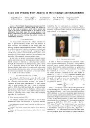
The Aibo robot from Sony (fig. 1) is a perfect
tool to implement and test artificial intelligent
techniques in robotics. The AIBO robot combines
a body (hardware) and mind (the Aibo Mind 3
software) that allow it to move, think, and display
the lifelike attribute of emotion, instinct, learning and
growth. It establishes communication with people by
displaying emotions, and assumes various behaviors
(autonomous actions) based on information which
it gathers from its environment. The Aibo robot
is not only a robot, but an autonomous robot with
the ability to complement your live. While living
with you, the behavior of the Aibo robot patterns
develops as it learns and grows. Also, it lets you to
implement new complex behaviors depending on the
environment. So it is the best tool to try and test a
signs recognition system in real environments. There
is no other so developed technology embedded in a
simple but intelligent robot.
Object recognition process basically is composed
by three steps: detection of a region of interest
(ROI), model matching, and classification. Each of
these steps can be done by a great different number
of algorithms. Depending on the object we want
to recognize, different techniques offer different
performance depending on the domain. Adaboost
[3] has been at last years one of the most used
Fig. 1. Sony Aibo robot.
technique for object detection, feature selection,
and object classification. Usually, the problem
of object recognition (e.g. person identification)
needs a previous addressing the category detection
(e.g. face location). According to the way objects
are described, three main families of approaches
can be considered [12]: part-based, patch-based
and region-based methods. Part-based approaches
consider that an object is defined as a specific
spatial arrangement of the object parts. An
unsupervised statistical learning of constellation
of parts and spatial relations is used in [10]. In
[11] and [13] a representation integrating Boosting
with constellations of contextual descriptors is
defined, where the feature vector includes the bins
that correspond to the different positions of the
correlograms determining the object properties.
Patch-based methods classify each rectangular
image region of a fixed aspect ratio (shape) at
multiple sizes, as object (or parts of the target object)
or background. In [9], objects are described by the
best features obtained using masks and normalized
cross-correlation. Finally, region-based algorithms
segment regions of the image from the background
and describe them by a set of features that provide
texture and shape information. In [11], the selection
of feature points is based on image contour points.
Model matching normally is adapted depending on
the domain we are working on, and finally, object
classification involves a lot of techniques to solve
the problem of discriminability between different
types of objects (classes).
When the number of classes to discriminate
are higher of two, the multiclass classification

JOSÉ LUIS LEDESMA PIQUERAS - REAL-TIME SIGN CLASSIFICATION FOR AIBO ROBOTS 3
is normally generated expending a set of twoclass
classifiers. The most common classifiers
used in the literature are: K-Nearest neighbors,
Principal Components Analysis, Fisher Discriminant
Analysis, Tangent Distance, Adaboost variants,
Support Vector Machine, etc.
In our application, we make use of the results of the
Adaboost procedure as a detection algorithm. The
use of this algorithm let us detect regions of interest
with high probability of containing signs. Once the
Adaboost returns a ROI, we fit the model using the
circular geometry properties, obtaining the estimated
center and the radius of the sign. The main reason
of using the circular geometry is the robustness of
the algorithm. Once we have fit the model, using
k-NN classification method we obtain the label of
the sign. We can use safely k-NN with the synthetic
signs we have created, because these signs are very
different between them. The system is validated
in a Sony Aibo robot showing good performance
on recognizing objects in real-time. In the next
part the methodology to solve a real traffic sign
recognition system is shown. All the algorithms used
are separately explained. Following one can read
about the results of applying the different algorithms.
This paper is organized as follows: Section 1
overviews robotics, artificial vision and introduces
the paper goal and scope. Section 2 describes the
required techniques of the methodology and it shows
the architecture of our proposed system. Section 3
shows the experiments and results, and section 4
concludes the paper.
II. METHODOLOGY
In this chapter, we explain the techniques used
to solve the model matching and classification of
objects. Finally, we show the integrated strategies in
the real application.
A. Adabost Detection
The AdaBoost boosting algorithm has become over
the last few years a very popular algorithm to use
in practice. The main idea of AdaBoost is to assign
each example of the given training set a weight. At
the beginning all weights are equal, but in every
round the weak learner returns a hypothesis, and
the weights of all examples classified wrong by that
hypothesis are increased. That way the weak learner
is forced to focus on the difficult examples of the
training set. The final hypothesis is a combination
of the hypotheses of all rounds, namely a weighted
majority vote, where hypotheses with lower classification
error have higher weight. Summarizing, the
approach consists of a) choosing a (weak) classifier,
b) modifying example weights in order to give priority
to examples where the previous classifiers fail,
and c) combining classifiers in a multiple classifier.
The combined classifier allows a good generalization
performance with the only requirement that each
weak learner obtains an accuracy better than random
[9]. The Adaboost procedure has been used for
feature selection, detection, and classification problems.
In our problem, the Gentle Adaboost has been
previously applied to detect the regions of interest
(ROI) with high probability of containing signs from
the Aibo video data. In fig. 2 the Gentle Adaboost
algorithm of our approach, that has been shown to
outperform the other Adaboost versions.
Fig. 2. Gentle Adaboost algorithm
In fig. 2, the weights of each of the samples
of the training set are initialized. Normally, the
same
weight is assigned to each sample satisfying
N
i=1 wi = 1. At iteration m of the algorithm, a
weak classifier evaluates the feature space and selects
the best feature based on the weights of the samples.
The samples are re-weighted with a exponential lossfunction,
and the process is repeated M times or
when the training classification error is zero. The
final strong classifier of the Gentle Adaboost algorithm
is an additive model that use a threshold as a
final classifier. To classify a new input, the results
of applying the m weak classifiers with the test
sample are added or subtracted depending on the
accuracy of each weak classifier. In the common
case of using decision stumps as a weak classifier,

JOSÉ LUIS LEDESMA PIQUERAS - REAL-TIME SIGN CLASSIFICATION FOR AIBO ROBOTS 4
the additive model assigns the same weight to each
of the hypothesis, so all the features are considered
to have the same importance. The last fact is the
main difference between the Gentle Adaboost and
the traditional Adaboost versions.
Given an Adaboost positive sample, it determines
a region of interest (ROI) that contains an object.
However, besides the ROI we miss information about
scale and position, so before applying recognition
we need to apply a spatial normalization. Concerned
with the correlation of sign distortion, we look for
affine transformations that can perform the spatial
normalization to improve final recognition.
B. Model fitting
In order to capture the model contained in the
detected ROI, we consider the radial properties of
the circular signs to fit a possible instance and to
estimate its center and radius.
Fast radial symmetry: The fast radial symmetry
[4] is calculated over a set of one or more ranges N
depending on the scale of the features one is trying to
detect. The value of the transform at range indicates
the contribution to radial symmetry of the gradients
a distance n away from each point. At each range
n we define an orientation projection image On (1)
and (2), generated by examining the gradient g at
each point p, from which a corresponding positivelyaffected
pixel p+ve(p) and negatively-affected pixel
p−ve(p) are determined (3) and (4).
On(P+ve(p)) = On(P+ve(p))+1 (1)
On(P−ve(p)) = On(P−ve(p))+1 (2)
P+ve(p) =p + round g(p)
n
||g(p)||
(3)
P−ve(p) =p − round g(p)
n (4)
||g(p)||
Now, to locate the radial symmetry position, we
search for the maximum position (x, y) at accumulated
orientations matrix OT :
O T n
=
(5)
On
i=1
Locating that maximum at the respective
orientation matrix, we determine the radius length.
This procedure allows to obtain robust results for
circular traffic signs fitting. An example is shown in
fig. 3.
The ROI that contains a circular sign may contain
noise inside and outside the object that can slightly
displace the center. To cope with this possible
displacement, we can iterate this procedure applying
a circular mask to exclude near points that can
displace the center of the sign, and repeat the
process limiting the radius range fig. 4.
Fig. 4. (a). Displaced center due to noise, and mask to exclude near points of
high gradient module. (b) Center correction from the next iteration of radial
symmetry.
C. Classification techniques
K-Nearest Neighbors: Among the various
methods of supervised statistical pattern recognition,
the Nearest Neighbour rule achieves consistently
high performance, without a priori assumptions
about the distributions from which the training
examples are drawn. It involves a training set of
both positive and negative cases. A new sample is
classified by calculating the distance to the nearest
training case; the sign of that point then determines
the classification of the sample. The k-NN classifier
extends this idea by taking the k nearest points and
assigning the sign of the majority. It is common to
select k small and odd to break ties (typically 1, 3 or
5). Larger k values help reduce the effects of noisy
points within the training data set, and the choice of
k is often performed through cross-validation. In this
way, given a input test sample vector of features x
of dimension n, we estimate its Euclidean distance d
(6) with all the training samples (y) and classify to
the class of the minimal distance.

JOSÉ LUIS LEDESMA PIQUERAS - REAL-TIME SIGN CLASSIFICATION FOR AIBO ROBOTS 5
(a) (b) (c) (d) (e) (f)
Fig. 3. (a) Input image, (b) X-derived, (c) Y-derived, (d) image gradient g, (e) total orientations accumulator matrix OT, (f) Captured center and radius.
n
d(x, y) = (xj − yj) 2 (6)
j=1
Principal Components Analysis: Principal
Component Analysis, from a statistical perspective,
is a method for transforming correlated variables into
uncorrelated variables, finding linear combinations
of the original variables with relatively large or
small variability, as well as for reducing data
dimensionality [5].
Given the set of N column vectors { −→ x i} of dimension
D, the mean of the data is:
−→
µ x = 1
N
−→
x i
(7)
N
i=1
The scatering total matrix is defined as:
ST = 1
N
(
N
i=1
−→ x i − −→ µ )( −→ x i − −→ µ ) T
(8)
We choose the eigenvectors of ST that correnpond
to the X% largest eigenvalues of ST to compute
Wpca, obtaining a transformation Xn ↦→ Y m , reducing
data of the form:
Y = Wpca(X − X) (9)
where X is the sample to project and X is the data
mean.
Fisher Linear Discriminant Analysis(FLDA):
Given the binary classification problem, FLDA
projects at one dimension each pair of classes
(reducing to C −1 where C is the number of classes),
multiplying each sample by its projection matrix,
which minimizes the distance between samples of
the same class, and maximizes the distance between
the two classes. The result is shown in fig. 5, where
the blue and red points belong to the samples of the
two projected classes, and the green line indicates
the threshold that best separates them [6].
Fig. 5. Fisher projection for two classes and threshold value.
The algorithm is as follows: Given the set of N
column vectors { −→ x i} of dimension D, we calculate
the mean of the data. For K classes C1,C2, ..., CK,
the mean of the class Ck that contains Nk elements is:
−→ µ xk = 1
xi
Nk −→
x i∈Ck
(10)
The separability maximization between classes is
defined as the quotient between the between-class
scatter matrix:
SB =
K
( −→ µ xk − −→ µ x)( −→ µ xk − −→ µ x) T
k=1
and the intra-class scatter matrix:
SW =
K
k=1 −→
x i∈Ck
( −→ x i − −→ µ xk)( −→ x i − −→ µ xk) T
The projection matrix W maximizes:
(11)
(12)
W T × SB × W
W T (13)
× SW × W
Let −→ w 1, ..., −→ w D be the generalized eigenvectors of
SB and SW . Then, selecting d

JOSÉ LUIS LEDESMA PIQUERAS - REAL-TIME SIGN CLASSIFICATION FOR AIBO ROBOTS 6
−→ T
y = W
−→
d x (14)
The generalized eigenvectors of (12) are the eigenvectors
of SBS −1
W .
D. System
In this section, we explain the architecture of the
whole application after integrating the previous techniques.
The scheme of the whole system is shown in
fig. 6.
The process starts with the autonomous Aibo robot
interaction, the captured frames are processed at the
detection step by the Gentle Adaboost Algorithm
(see appendix E). The detected ROIs with a high
probability of containing a circular sign are sent to
our system to proceed with the model fitting and
posterior classification. First, fast radial symmetry
is applied to the ROI, and if the specifications succeed,
the captured region is normalized previously
to classify (see results section). At the classification
step, k − NN and Fisher Linear Discriminant Analysis
with a previous Principal Components Analysis
(FLDA) depending on the type of the fitted object is
applied.
III. RESULTS
Aibo has a VGA quality camera, which gives a
maximum resolution of 640×480. Once the image is
captured, and after converting the image to greyscale,
the Adaboost algorithm is applied to detect all the
ROIs, that are the inputs of our system.
A. Model matching parameters
Given an Adaboost image, it determines a region
of interest that contains a sign. Still, given the
ROI we miss information about the sign scale
and position, so before applying recognition we
need to apply a spatial normalization. Concerned
with the correlation of sign distortion, we look for
affine transformations that can perform the spatial
normalization to improve final recognition.
First, all the points in the image are treated in the
same way. We get the module and the derivative of
each point of the image projecting it for different
radius values to find the center. These initial radius
estimates are from 20% to 50% of the image height.
The only procedure we apply in this first step is
a simple threshold to try to determine if the point
we are working on is part of the boundary of the
sign. This threshold is determined by the 10% of
the gradient image max value. Once the algorithm is
applied for first time, we have the object center and
radius, probably affected by the noise of the image.
In order to make a better approximation, a mask
over the center of the estimated sign is applied, that
avoids the effect of the inner-sign noise. To prevent
the possible previous displacement of the containing
noise, and to remove the inner-sign noise by means
of the mask, instead of using a large number of
radius to determine the center, we also limit the
number of radius we use. So, in this second time we
apply this algorithm we use a radius from 80% to
the 120% of the previous calculated radius. In fact,
we are using the same algorithm all the time, but
limiting the importance of each point in the image,
to fit the real center and radius of the sign limiting
the center searching and avoiding the effect of the
typical noise of real images.
In some cases, the ROIs obtained by the use of
the Gentle Adaboost algorithm can be false positives
(regions detected with as probability of containing a
sign that really corresponds to background regions).
Besides to optimize the model fitting, we approximate
a new methodology to detect false positives.
To avoid this problem, as we know some a priori
characteristics about the object representation, we
can use that properties to detect false regions. We
know that the center of the sign will be more or
less at the center of the image, and also that the
radius is approximately 2/3 of the height of the
image. In this way, any sign detected that did not
match these basic characteristics is a false positive.
In this way, the false positives detection is based on
estimating the theshold values to avoid false positives
based on (eq.15), where C = (cx,cy) corresponds
to the center position, h and w correspond to the
height and width of the ROI, and cx1 and cy1 are the
intervals to consider a positive possible estimation of
the center for a real sign. For the radius threshold,
the restriction is based in obtaining a radius value R
h , 1.5 ],thus leading to:
2
between the interval [0.5 h
2

JOSÉ LUIS LEDESMA PIQUERAS - REAL-TIME SIGN CLASSIFICATION FOR AIBO ROBOTS 7
Fig. 6. Whole intelligent Aibo process scheme.
cy1 ∈ [0.6 h
, 1.4h
2 2 ],cx1 ∈ [0.6 x
, 1.4x ] (15)
2 2
Once we have a good approximation about the
center and the radius of the circular sign, we have
to normalize it before classification.
B. Normalization parameters
The normalization process consists in four steps.
First we rescale it to a 30 × 30 pixels image. Secondly
we equalize the image. When one wishes to
compare two or more images on a specific basis,
such as texture, it is common to first normalize their
histograms to a ”standard” histogram. This can be
especially useful when the images have been acquired
under different circumstances. The most common
histogram normalization technique is histogram
equalization where one attempts to change the histogram
through the use of a function b = f(a) into
a histogram that is constant for all brightness values.
This would correspond to a brightness distribution
where all values are equally probable. Unfortunately,
for an arbitrary image, one can only approximate
this result. For a ”suitable” function f(∗) the relation
between the input probability density function, the
output probability density function, and the function
f(∗) is given by:
pb(b)db = pa(a)da =⇒ df = pa(a)da
(16)
pb(d)
From (16) we see that ”suitable” means that f(∗)
is differentiable and that df/da ≧ 0. For histogram
equalization we desire that pb(b) = constant and
this means that:
f(a) =(2 B − 1) × p(a) (17)
where P (a) is the probability distribution function.
In other words, the quantized probability distribution
function normalized from 0 to 2B − 1 is the lookup
table required for histogram equalization. The
histogram equalization procedure can also be applied
on a regional basis.
The regions of the sign are not homogeneous,
so, classification methods could accumulate errors.
To solve this problem, we use different anisotropic
filters, Perona and Malik [7] and Weickert [8], and
we observed that Weickert filter runs better on our
images. Anisotropic filtering is a technique designed
to sharpen the textures that appear on surfaces. It
works by taking multiple bi-linear or tri-linear texture
samples for each pixel, which prevents the blurriness
that normally results from textures rendered at
sharp angles relative to the viewer. The reason these
textures appear blurry is because a single pixel on
an angled surface covers a large amount of surface
area relative to a pixel on a surface viewed straight
on. This means that many more texels will lie in the
vicinity of the pixel center, and their values need to
be taken into account to accurately determine the
pixel color. Rather than just sampling the nearest
texels to the pixel center, anisotropic filtering takes
additional samples along the slope of the surface.
The more strongly sloped the surface is, the more
samples will be necessary to maintain image fidelity.
In general, 16 samples are sufficient to eliminate any
visible blurriness on even the most extremely angled
surfaces and mask the image to have visible only the
part of the ROI we are interested in: the sign. The
result is shown in fig. 7.

JOSÉ LUIS LEDESMA PIQUERAS - REAL-TIME SIGN CLASSIFICATION FOR AIBO ROBOTS 8
(a) (b)
Fig. 7. (a) Extracted equalized sign. (b) Anisotropic Weickert filter.
C. Database generation
The database we have used is based on over 500
images of each class, generated and stored using the
previous procedures. Much more images will lead to
a slower system performance, and less images will
reduce the percentage of success. In the k-NN application,
a k = 3 has obtained a good performance
as the number of nearest neighbors considered to
classify a given object. The three-class Aibo problem
representant are shown in fig. 8.
Fig. 8. Aibo circular classes.
D. Classification parameters
Now that we have the image normalized, the
classification algorithm (k-NN) has to deal with a
3-class to return the sign label.
The k-NN algorithm compares each image it
has stored in its database, with the image we have
obtained from the model matching. A good database,
and a good K election will determine the success of
the classification. To determine the real success of
the application, each part of it has been accurately
tested. For the model matching we have used 500
images, from which the system has returned a 97.4%
of success. Whilst the system, at first sight, should
return a 100% success, some images are difficult to
treat, even for the human eye, as we can see in the
fig. 9.
Fig. 9. Difficult captured sign.
The image of fig. 9 shows a difficult image to wellrecognize
due to the real behavior of Aibo in noncontrolled
environments. In order to test the classification,
we used a ten-fold cross-validation, with a
confidence range of 99% interval. We have gotten
over 1000 images, and 10 groups of 100 images
were made. We use 9 of these groups to train the
classification system, and the other one to test it, and
we repeated this process ten times. Once we have
done the 10 validations, we obtained a 96.2±1.02%
average. We calculate the confidence interval by:
std(P )
R =1.96 × 1 n
(18)
n j=1 P (j)
where P is the vector with the n classification
iterations, R is the confidence interval, and std is
the standard deviation. After this test, we obtained
that the whole system has a performance of 93.69%
success, which, up to our opinion, is highly robust
taking in to account that the application is running in
a non-controlled environments. In fig. 10 a process
of a synthetic Aibo image to fit the model is shown,
and fig. 11 shows the normalized image.
Fig. 11. Normalized-rescaled Aibo recognized sign.
E. Real traffic sign recognition system
In order to test the robustness of our system in
real application, we have applied it to a real traffic
sign recognition system. This test allowed us not
only to work in a real non-controlled system, but
also to work with real objects (non synthetic ones
as in the previous case) that can appear in different
conditions, and with different appearance. In this

JOSÉ LUIS LEDESMA PIQUERAS - REAL-TIME SIGN CLASSIFICATION FOR AIBO ROBOTS 9
Fig. 10. Synthetic image fitting.
Fig. 12. Real traffic sign circular classes.
Fig. 13. Real traffic sign speed classes.
way, a new problem is introduced: not all the objects
are enough discriminable and some of them share
similar features, so it is more difficult to obtain a
high recognition performance. In fig. 12 and 13,
the different classes of speed signs are shown. Each
speed sign is very close to the others, that makes
more difficult the work of k-NN since slight movements
can introduces high correlation errors. We
have also used FLDA (with a previous 99.99% of
PCA) to obtain a more sophisticated classification
comparative since FLDA is known to work with a
data projection with a previous training that estimate
a matrix projection that optimally split the samples.
FLDA is a one-versus-one class algorithm, so we
have used a pairwise voting system, to extend the
FLDA as a binary classifier to a multiclass problem.
The voting scheme (pairwise) uses a matrix of dimension
Nc ×Nc, where Nc is the number of classes.
Each position for a test input sample corresponds to
the class with a high membership probability using
classifier that trains class of row i versus class of
column j. In this way, in the final tested matrix the
maximal voting value for a class corresponds to the
classification label.
The circular group is treated in the same way that
the synthetic Aibo images. For the speed group we
applied a normalization strategy. As the speed group
does not have intermediate level of greys levels, it
is better to binarize the regions to avoid the error
that can be accumulated by false grey levels that
can appear due to different conditions as shadows.
In fig. 15 different signs extracted from 1024×1024
real images at different real conditions are shown
to observe the difficulty to classify in these adverse
conditions.
In this way, when we receive a ROI from the
Adaboost procedure obtained by the training of
real images, the ROI is fitted with the optimized
fast radial symmetry, and classified. In case to be
classified by the speed group (with a class that
contains all the speed classes together), a new
classification is done with a new binary database of
speed classes with the two different classification
strategies. Fig. 14 shows the new scheme adapted
to the real sign recognition system, where one can
see the different treatment when a speed sign is
classified. The data used for this test is a set of 200
real samples for the circular group and the same
number of samples for the real speed classes.
As we can see in the table I, k-NN and FLDA are
very near in success where we are treating with welldiscriminate
classes, although in this case FLDA
allow us to classify more quickly by the fact that we
only need a multiplication and threshold comparison
instead to compare with all the stored images of
the database classes. When we are working with
very similar classes, the k-NN algorithm looses a
lot of precision, meanwhile FLDA treated with them
with a great success, as the results and confidence

JOSÉ LUIS LEDESMA PIQUERAS - REAL-TIME SIGN CLASSIFICATION FOR AIBO ROBOTS 10
Fig. 14. Real traffic sign system scheme.
Fig. 15. Different ROIs of real traffic sign at different real conditions.
Circular group Speed group
k-NN 92.73±1.02 71.14±1.70
FLDA 93.12±0.13 87.18±1.30
TABLE I
CLASSIFICATION RESULTS FOR k-NN AND FLDA FOR THE REAL TRAFFIC
SIGN GROUPS.
intervals show. The results are also graphically
showed in fig. 18 and 19.
F. Discussion
In this chapter, we have exposed two different
types of experiments. First, the performance for the
detection, model matching and classification of the
Sony Aibo robot has been shown. The system shows
high accuracy with the generated synthetic objects
in real non-controlled environments. The k-NN
classification technique is a good option due to the
high discriminability between classes. The databases
do not need aN excessive number of classes and the
real-time performance is allowed.
The second experiment is a real validation of
the application in a real traffic sign recognition
system. This experiment has been done in order
to validate the performance of our approaches in
environments with difficult conditions to treat. The
signs to recognize are less discriminable and they
appear in adverse conditions. We have observed
that the speed classes require a concrete pre-process
to improve the classification step. Due to the low
performance of the k-NN strategy at the speed
classes, new classification techniques have been
required to increase the performance of the process.
We have used Fisher Linear Discriminant Analysis
with a previous Principal Components Analysis to
not use the local-behavior of the k-NN correlation
scheme. The projection allowed by FLDA allow
us to increase the performance and obtain robust
results. In fig. 16 an example of a whole traffic
sign captured image and the region of interest that
contains a circular sign are shown, and the fig. 17
shows an example of the execution of our process
in the Aibo system, where an interface shows the
frame captured by the image and the recognized sign.
Fig. 16. Real traffic sign image.
IV. CONCLUSIONS
Recently, intelligent robotics and computer vision
have shown significant advances. Normally, the design
depends on a concrete problem domain. The
Sony Aibo robot is a useful robotic tool to test developed
systems on real environments. In this paper, we

JOSÉ LUIS LEDESMA PIQUERAS - REAL-TIME SIGN CLASSIFICATION FOR AIBO ROBOTS 11
Fig. 17. Aibo system interaction and recognition interface.
have designed a real application to make Aibo recognize
synthetic circular objects in cluttered scenes.
We developed a robust system to solve the problem
of model matching and object classification. The
first approach includes well-differentiated synthetic
objects, where Aibo shows a high recognition and
autonomous behavior performance. After that, we
extended the use of the system in a real traffic sign
recognition process, proving the robustness of the
system recognizing different types of traffic signs
at different non-controlled conditions, showing the
flexibility and robustness of our application either in
case of lack of visibility, partial occlusions, noise,
and slight affine transformations.
Fig. 18. Classification accuracy for the real circular group using k-NN and
FLDA.
V. ACKNOWLEDGEMENTS
I want to acknowledge Sergio Escalera and Petia
Radeva the direction in this project. It would not have
been possible to develop the project without them.
I want to acknowledge the essencial aportation of
Fig. 19. Classification accuracy for the real speed group using k-NN and
FLDA.
Xavi, Carlos and Raul. I want also to acknowledge
my parents and family for helping me, not only
during the realization of this project, but also in my
general life. I would also acknowledge all my friends
that have stand me in the worst moments, with a very
special mention to Sergio, Tania, Annita, Dunia and
Gomez. Thanks for being near me always I need you.
REFERENCES
[1] Yoav Freund and Robert E. Schapire. ”A decision-theoretic generalization
online learning and an application to boosting,” Computational Learning
Theory: Eurocolt ’95, pages 23-37. Springer-Verlag, 1995.
[2] Paul Viola and Michael J. Jones, ”Robust Real-time Object Detection,”
Cambridge Research Laboratory, Technical Report Series, CRL 2001/01.
Feb. 2001.
[3] J. Friedman, T. Hastie, and R. Tibshirani, ”Additive logistic regression: a
statistical view of boosting”, Technical Report, 1998.
[4] G. Loy, and A. Zelinsky, ”A Fast Radial Symmetry Transform for
Detecting Points of Interest”, Transactions on PAMI, 2003.
[5] Lindsay I Smith , ”A tutorial on Principal Components Analysis”,
February, 2002
[6] MaxWelling , ”Fisher Linear Discriminant Analysis”, Department of
Computer Science, University of Toronto, 2002.
[7] Perona P., Malik J., ”Scale space and edge detection using anisotropic
diffusion”, IEEE Trans. Pattern Anal. Machine Intell., Vol. 12, pp. 629-
639, July 1990.
[8] Weickert J., ”Anisotropic diffusion in image processing”, European Consortium
for Mathematics in Industry (B.G. Teubner,Stuttgart), 1998.
[9] A. Torralba, K. Murphy and W. Freeman, ”Sharing Visual Features for
Multiclass and Multiview Object Detection”, CVPR, pp. 762-769, vol. 2,
2004.
[10] R. Fergus, P. Perona, and A. Zisserman, ”Object class recognition by
unsupervised scale-invariant learning”, CVPR, 2003.
[11] J. Amores, N. Sebe and P. Radeva, ”Fast Spatial Pattern Discovery
Integrating Boosting with Constellations of Contextual Descriptors”,
CVPR, 2005.
[12] K. Murphy, A.Torralba and W.T.Freeman, ”Using the Forest to See
the Trees: A Graphical Model Relating Features, Objects, and Scenes”,
Advances in NIPS, MIT Press, 2003.
[13] S. Escalera, O. Pujol, and P. Radeva, ”Boosted Landmarks of contextual
descriptors and Forest-ECOC: A novel framework to detect and classify
objects in cluttered scenes”, International Conference on Pattern Recognition,
Hong Kong, 2006.

Appendices
To complement the information of the project that can not be included in the article,
some appendices have been included. In order to explain in more detail the domain
of the work, first appendix is related to the Artificial Intelligence History. In the
topic of Artificial Intelligence, we have basically focused on Artificial Vision, so the
next appendix is an overview of Computer Vision. The following two appendices
explain the origin of the real traffic sign data that we process in this work, and the
technics specifications of the Sony Aibo robot as the autonomous system used in
the project. Finally, the source code of the application is shown.
24
12

Appendix A. Artificial Intelligence
history
Prehistory of AI
Humans have always speculated about the nature of mind, thought, and language,
and searched for discrete representations of their knowledge. Aristotle tried to formalize
this speculation by means of syllogistic logic, which remains one of the key
strategies of AI. The first is-a hierarchy was created in 260 by Porphyry of Tyros.
Classical and medieval grammarians explored more subtle features of language that
Aristotle shortchanged, and mathematician Bernard Bolzano made the first modern
attempt to formalize semantics in 1837.
Early computer design was driven mainly by the complex mathematics needed to
target weapons accurately, with analog feedback devices inspiring an ideal of cybernetics.
The expression ”artificial intelligence” was introduced as a ’digital’ replacement
for the analog ’cybernetics’.
Development of AI theory
Much of the (original) focus of artificial intelligence research draws from an experimental
approach to psychology, and emphasizes what may be called linguistic
intelligence (best exemplified in the Turing test).
Approaches to Artificial Intelligence that do not focus on linguistic intelligence include
robotics and collective intelligence approaches, which focus on active manipulation
of an environment, or consensus decision making, and draw from biology and
political science when seeking models of how ”intelligent” behavior is organized.
AI also draws from animal studies, in particular with insects, which are easier to
emulate as robots (see artificial life), as well as animals with more complex cognition,
including apes, who resemble humans in many ways but have less developed
capacities for planning and cognition. Some researchers argue that animals, which
are apparently simpler than humans, ought to be considerably easier to mimic. But
satisfactory computational models for animal intelligence are not available.
Seminal papers advancing AI include ”A Logical Calculus of the Ideas Immanent in
Nervous Activity” (1943), by Warren McCulloch and Walter Pitts, and ”On Computing
Machinery and Intelligence” (1950), by Alan Turing, and ”Man-Computer
Symbiosis” by J.C.R. Licklider. See Cybernetics and Turing test for further discussion.
There were also early papers which denied the possibility of machine intelligence on
logical or philosophical grounds such as ”Minds, Machines and Gödel” (1961) by
John Lucas.
With the development of practical techniques based on AI research, advocates of
10
13

AI have argued that opponents of AI have repeatedly changed their position on
tasks such as computer chess or speech recognition that were previously regarded
as ”intelligent” in order to deny the accomplishments of AI. Douglas Hofstadter,
in Gödel, Escher, Bach, pointed out that this moving of the goalposts effectively
defines ”intelligence” as ”whatever humans can do that machines cannot”.
John von Neumann (quoted by E.T. Jaynes) anticipated this in 1948 by saying, in
response to a comment at a lecture that it was impossible for a machine to think:
”You insist that there is something a machine cannot do. If you will tell me precisely
what it is that a machine cannot do, then I can always make a machine which
will do just that!”. Von Neumann was presumably alluding to the Church-Turing
thesis which states that any effective procedure can be simulated by a (generalized)
computer.
In 1969 McCarthy and Hayes started the discussion about the frame problem with
their essay, ”Some Philosophical Problems from the Standpoint of Artificial Intelligence”.
Experimental AI research
Artificial intelligence began as an experimental field in the 1950s with such pioneers
as Allen Newell and Herbert Simon, who founded the first artificial intelligence
laboratory at Carnegie Mellon University, and John McCarthy and Marvin Minsky,
who founded the MIT AI Lab in 1959. They all attended the Dartmouth College
summer AI conference in 1956, which was organized by McCarthy, Minsky, Nathan
Rochester of IBM and Claude Shannon.
Historically, there are two broad styles of AI research - the ”neats” and ”scruffies”.
”Neat”, classical or symbolic AI research, in general, involves symbolic manipulation
of abstract concepts, and is the methodology used in most expert systems. Parallel
to this are the ”scruffy”, or ”connectionist”, approaches, of which artificial neural
networks are the best-known example, which try to ”evolve” intelligence through
building systems and then improving them through some automatic process rather
than systematically designing something to complete the task. Both approaches appeared
very early in AI history. Throughout the 1960s and 1970s scruffy approaches
were pushed to the background, but interest was regained in the 1980s when the
limitations of the ”neat” approaches of the time became clearer. However, it has
become clear that contemporary methods using both broad approaches have severe
limitations.
Artificial intelligence research was very heavily funded in the 1980s by the Defense
Advanced Research Projects Agency in the United States and by the fifth generation
computer systems project in Japan. The failure of the work funded at the
time to produce immediate results, despite the grandiose promises of some AI practitioners,
led to correspondingly large cutbacks in funding by government agencies
in the late 1980s, leading to a general downturn in activity in the field known as AI
winter. Over the following decade, many AI researchers moved into related areas
with more modest goals such as machine learning, robotics, and computer vision,
11
14

though research in pure AI continued at reduced levels.
Micro-World AI
The real world is full of distracting and obscuring detail: generally science progresses
by focusing on artificially simple models of reality (in physics, frictionless planes and
perfectly rigid bodies, for example). In 1970 Marvin Minsky and Seymour Papert,
of the MIT AI Laboratory, proposed that AI research should likewise focus on
developing programs capable of intelligent behaviour in artificially simple situations
known as micro-worlds. Much research has focused on the so-called blocks world,
which consists of coloured blocks of various shapes and sizes arrayed on a flat surface.
Micro-World AI
Spinoffs
Whilst progress towards the ultimate goal of human-like intelligence has been slow,
many spinoffs have come in the process. Notable examples include the languages
LISP and Prolog, which were invented for AI research but are now used for non-AI
tasks. Hacker culture first sprang from AI laboratories, in particular the MIT AI
Lab, home at various times to such luminaries as John McCarthy, Marvin Minsky,
Seymour Papert (who developed Logo there) and Terry Winograd (who abandoned
AI after developing SHRDLU).
AI languages and programming styles
AI research has led to many advances in programming languages including the first
list processing language by Allen Newell et. al., Lisp dialects, Planner, Actors, the
Scientific Community Metaphor, production systems, and rule-based languages.
GOFAI TEST research is often done in programming languages such as Prolog
or Lisp. Bayesian work often uses Matlab or Lush (a numerical dialect of Lisp).
These languages include many specialist probabilistic libraries. Real-life and especially
real-time systems are likely to use C++. AI programmers are often academics
and emphasise rapid development and prototyping rather than bulletproof software
engineering practices, hence the use of interpreted languages to empower rapid
command-line testing and experimentation.
The most basic AI program is a single If-Then statement, such as ”If A, then B.”
If you type an ’A’ letter, the computer will show you a ’B’ letter. Basically, you are
teaching a computer to do a task. You input one thing, and the computer responds
with something you told it to do or say. All programs have If-Then logic. A more
complex example is if you type in ”Hello.”, and the computer responds ”How are
you today?” This response is not the computer’s own thought, but rather a line you
wrote into the program before. Whenever you type in ”Hello.”, the computer always
responds ”How are you today?”. It seems as if the computer is alive and thinking
to the casual observer, but actually it is an automated response. AI is often a long
series of If-Then (or Cause and Effect) statements.
12
15

A randomizer can be added to this. The randomizer creates two or more response
paths. For example, if you type ”Hello”, the computer may respond with ”How
are you today?” or ”Nice weather” or ”Would you like to play a game?” Three
responses (or ’thens’) are now possible instead of one. There is an equal chance
that any one of the three responses will show. This is similar to a pull-cord talking
doll that can respond with a number of sayings. A computer AI program can have
thousands of responses to the same input. This makes it less predictable and closer to
how a real person would respond, arguably because living people respond somewhat
unpredictably. When thousands of input (”if”) are written in (not just ”Hello.”) and
thousands of responses (”then”) are written into the AI program, then the computer
can talk (or type) with most people, if those people know the If statement input
lines to type.
Many games, like chess and strategy games, use action responses instead of typed
responses, so that players can play against the computer. Robots with AI brains
would use If-Then statements and randomizers to make decisions and speak. However,
the input may be a sensed object in front of the robot instead of a ”Hello.”
line, and the response may be to pick up the object instead of a response line.
Chronological History
Historical Antecedents
Greek myths of Hephaestus and Pygmalion incorporate the idea of intelligent robots.
In the 5th century BC, Aristotle invented syllogistic logic, the first formal deductive
reasoning system.
Ramon Llull, Spanish theologian, invented paper ”machines” for discovering nonmathematical
truths through combinattions of words from lists in the 13th century.
By the 15th century and 16th century, clocks, the first modern measuring machines,
were first produced using lathes. Clockmakers extended their craft to creating mechanical
animals and other novelties. Rabbi Judah Loew ben Bezalel of Prague is
said to have invented the Golem, a clay man brought to life (1580).
Early in the 17th century, René Descartes proposed that bodies of animals are
nothing more than complex machines. Many other 17th century thinkers offered
variations and elaborations of Cartesian mechanism. Thomas Hobbes published
Leviathan, containing a material and combinatorial theory of thinking. Blaise Pascal
created the second mechanical and first digital calculating machine (1642). Gottfried
Leibniz improved Pascal’s machine, making the Stepped Reckoner to do multiplication
and division (1673) and evisioned a universal calculus of reasoning (Alphabet
of human thought) by which arguments could be decided mechanically.
The 18th century saw a profusion of mechanical toys, including the celebrated mechanical
duck of Jacques de Vaucanson and Wolfgang von Kempelen’s phony chessplaying
automaton, The Turk (1769).
13
16

Mary Shelley published the story of Frankenstein; or the Modern Prometheus (1818).
19th and Early 20th Century
George Boole developed a binary algebra (Boolean algebra) representing (some)
”laws of thought.” Charles Babbage and Ada Lovelace worked on programmable
mechanical calculating machines.
In the first years of the 20th century Bertrand Russell and Alfred North Whitehead
published Principia Mathematica, which revolutionized formal logic. Russell,
Ludwig Wittgenstein, and Rudolf Carnap lead philosophy into logical analysis of
knowledge. Karel Capek’s play R.U.R. (Rossum’s Universal Robots)) opens in London
(1923). This is the first use of the word ”robot” in English.
Mid 20th century and Early AI
Warren Sturgis McCulloch and Walter Pitts publish ”A Logical Calculus of the
Ideas Immanent in Nervous Activity” (1943), laying foundations for artificial neural
networks. Arturo Rosenblueth, Norbert Wiener and Julian Bigelow coin the term
”cybernetics” in a 1943 paper. Wiener’s popular book by that name published in
1948. Vannevar Bush published As We May Think (The Atlantic Monthly, July
1945) a prescient vision of the future in which computers assist humans in many
activities.
The man widely acknowledged as the father of computer science, Alan Turing, published
”Computing Machinery and Intelligence” (1950) which introduced the Turing
test as a way of operationalizing a test of intelligent behavior. Claude Shannon published
a detailed analysis of chess playing as search (1950). Isaac Asimov published
his Three Laws of Robotics (1950).
1956: John McCarthy coined the term ”artificial intelligence” as the topic of the
Dartmouth Conference, the first conference devoted to the subject.
Demonstration of the first running AI program, the Logic Theorist (LT) written by
Allen Newell, J.C. Shaw and Herbert Simon (Carnegie Institute of Technology, now
Carnegie Mellon University).
1957: The General Problem Solver (GPS) demonstrated by Newell, Shaw and Simon.
1952-1962: Arthur Samuel (IBM) wrote the first game-playing program, for checkers
(draughts), to achieve sufficient skill to challenge a world champion. Samuel’s machine
learning programs were responsible for the high performance of the checkers
player.
1958: John McCarthy (Massachusetts Institute of Technology or MIT) invented
the Lisp programming language. Herb Gelernter and Nathan Rochester (IBM) described
a theorem prover in geometry that exploits a semantic model of the domain
in the form of diagrams of ”typical” cases. Teddington Conference on the Mechanization
of Thought Processes was held in the UK and among the papers presented
14
17

were John McCarthy’s Programs with Common Sense, Oliver Selfridge’s Pandemonium,
and Marvin Minsky’s Some Methods of Heuristic Programming and Artificial
Intelligence.
Late 1950s and early 1960s: Margaret Masterman and colleagues at University of
Cambridge design semantic nets for machine translation.
1961: James Slagle (PhD dissertation, MIT) wrote (in Lisp) the first symbolic integration
program, SAINT, which solved calculus problems at the college freshman
level.
1962: First industrial robot company, Unimation, founded.
1963: Thomas Evans’ program, ANALOGY, written as part of his PhD work at
MIT, demonstrated that computers can solve the same analogy problems as are
given on IQ tests. Edward Feigenbaum and Julian Feldman published Computers
and Thought, the first collection of articles about artificial intelligence.
1964: Danny Bobrow’s dissertation at MIT (technical report #1 from MIT’s AI
group, Project MAC), shows that computers can understand natural language well
enough to solve algebra word problems correctly. Bert Raphael’s MIT dissertation
on the SIR program demonstrates the power of a logical representation of knowledge
for question-answering systems.
1965: J. Alan Robinson invented a mechanical proof procedure, the Resolution
Method, which allowed programs to work efficiently with formal logic as a representation
language. Joseph Weizenbaum (MIT) built ELIZA (program), an interactive
program that carries on a dialogue in English language on any topic. It was
a popular toy at AI centers on the ARPANET when a version that ”simulated” the
dialogue of a psychotherapist was programmed.
1966: Ross Quillian (PhD dissertation, Carnegie Inst. of Technology, now CMU)
demonstrated semantic nets. First Machine Intelligence workshop at Edinburgh: the
first of an influential annual series organized by Donald Michie and others. Negative
report on machine translation kills much work in Natural language processing (NLP)
for many years.
1967: Dendral program (Edward Feigenbaum, Joshua Lederberg, Bruce Buchanan,
Georgia Sutherland at Stanford University) demonstrated to interpret mass spectra
on organic chemical compounds. First successful knowledge-based program for
scientific reasoning. Joel Moses (PhD work at MIT) demonstrated the power of
symbolic reasoning for integration problems in the Macsyma program. First successful
knowledge-based program in mathematics. Richard Greenblatt (programmer)
at MIT built a knowledge-based chess-playing program, MacHack, that was
good enough to achieve a class-C rating in tournament play.
1968: Marvin Minsky and Seymour Papert publish Perceptrons, demonstrating limits
of simple neural nets.
15
18

1969: Stanford Research Institute (SRI): Shakey the Robot, demonstrated combining
animal locomotion, perception and problem solving. Roger Schank (Stanford)
defined conceptual dependency model for natural language understanding. Later
developed (in PhD dissertations at Yale University) for use in story understanding
by Robert Wilensky and Wendy Lehnert, and for use in understanding memory by
Janet Kolodner. Yorick Wilks (Stanford) developed the semantic coherence view of
language called Preference Semantics, embodied in the first semantics-driven machine
translation program, and the basis of many PhD dissertations since such as
Bran Boguraev and David Carter at Cambridge. First International Joint Conference
on Artificial Intelligence (IJCAI) held at Stanford.
1970: Jaime Carbonell (Sr.) developed SCHOLAR, an interactive program for computer
assisted instruction based on semantic nets as the representation of knowledge.
Bill Woods described Augmented Transition Networks (ATN’s) as a representation
for natural language understanding. Patrick Winston’s PhD program, ARCH, at
MIT learned concepts from examples in the world of children’s blocks.
Early 70’s: Jane Robinson and Don Walker established an influential Natural Language
Processing group at SRI.
1971: Terry Winograd’s PhD thesis (MIT) demonstrated the ability of computers to
understand English sentences in a restricted world of children’s blocks, in a coupling
of his language understanding program, SHRDLU, with a robot arm that carried
out instructions typed in English.
1972: Prolog programming language developed by Alain Colmerauer.
1973: The Assembly Robotics Group at University of Edinburgh builds Freddy
Robot, capable of using visual perception to locate and assemble models. The
Lighthill report gives a largely negative verdict on AI research in Great Britain
and forms the basis for the decision by the British government to discontine support
for AI research in all but two universities.
1974: Ted Shortliffe’s PhD dissertation on the MYCIN program (Stanford) demonstrated
the power of rule-based systems for knowledge representation and inference
in the domain of medical diagnosis and therapy. Sometimes called the first expert
system. Earl Sacerdoti developed one of the first planning programs, ABSTRIPS,
and developed techniques of hierarchical planning.
1975: Marvin Minsky published his widely-read and influential article on Frames as a
representation of knowledge, in which many ideas about schemas and semantic links
are brought together. The Meta-Dendral learning program produced new results in
chemistry (some rules of mass spectrometry) the first scientific discoveries by a
computer to be published in a referreed journal.
Mid 70’s: Barbara Grosz (SRI) established limits to traditional AI approaches to
discourse modeling. Subsequent work by Grosz, Bonnie Webber and Candace Sidner
developed the notion of ”centering”, used in establishing focus of discourse and
16
19

anaphoric references in NLP. David Marr and MIT colleagues describe the ”primal
sketch” and its role in visual perception.
1976: Douglas Lenat’s AM program (Stanford PhD dissertation) demonstrated the
discovery model (loosely-guided search for interesting conjectures). Randall Davis
demonstrated the power of meta-level reasoning in his PhD dissertation at Stanford.
Late 70’s: Stanford’s SUMEX-AIM resource, headed by Ed Feigenbaum and Joshua
Lederberg, demonstrates the power of the ARPAnet for scientific collaboration.
1978: Tom Mitchell, at Stanford, invented the concept of Version Spaces for describing
the search space of a concept formation program. Herbert Simon wins the Nobel
Prize in Economics for his theory of bounded rationality, one of the cornerstones of
AI known as ”satisficing”. The MOLGEN program, written at Stanford by Mark
Stefik and Peter Friedland, demonstrated that an object-oriented programming representation
of knowledge can be used to plan gene-cloning experiments.
1979: Bill VanMelle’s PhD dissertation at Stanford demonstrated the generality
of MYCIN’s representation of knowledge and style of reasoning in his EMYCIN
program, the model for many commercial expert system ”shells”. Jack Myers and
Harry Pople at University of Pittsburgh developed INTERNIST, a knowledge-based
medical diagnosis program based on Dr. Myers’ clinical knowledge. Cordell Green,
David Barstow, Elaine Kant and others at Stanford demonstrated the CHI system
for automatic programming. The Stanford Cart, built by Hans Moravec, becomes
the first computer-controlled, autonomous vehicle when it successfully traverses a
chair-filled room and circumnavigates the Stanford AI Lab. Drew McDermott and
Jon Doyle at MIT, and John McCarthy at Stanford begin publishing work on nonmonotonic
logics and formal aspects of truth maintenance.
1980s: Lisp machines developed and marketed. First expert system shells and commercial
applications.
1980: Lee Erman, Rick Hayes-Roth, Victor Lesser and Raj Reddy published the first
description of the blackboard model, as the framework for the HEARSAY-II speech
understanding system. First National Conference of the American Association for
Artificial Intelligence (AAAI) held at Stanford.
1981: Danny Hillis designs the connection machine, a massively parallel architecture
that brings new power to AI, and to computation in general. (Later founds Thinking
Machines, Inc.)
1982: The Fifth Generation Computer Systems project (FGCS), an initiative by
Japan’s Ministry of International Trade and Industry, begun in 1982, to create a
”fifth generation computer” (see history of computing hardware) which was supposed
to perform much calculation utilizing massive parallelism.
1983: John Laird and Paul Rosenbloom, working with Allen Newell, complete CMU
dissertations on Soar (program). James F. Allen invents the Interval Calculus, the
17
20

first widely used formalization of temporal events.
Mid 80’s: Neural Networks become widely used with the Backpropagation algorithm
(first described by Paul Werbos in 1974).
1985: The autonomous drawing program, AARON, created by Harold Cohen, is
demonstrated at the AAAI National Conference (based on more than a decade of
work, and with subsequent work showing major developments).
1987: Marvin Minsky publishes The Society of Mind, a theoretical description of
the mind as a collection of cooperating agents.
1989: Dean Pomerleau at CMU creates ALVINN (An Autonomous Land Vehicle
in a Neural Network), which grew into the system that drove a car coast-to-coast
under computer control for all but about 50 of the 2850 miles.
1990s: Major advances in all areas of AI, with significant demonstrations in machine
learning, intelligent tutoring, case-based reasoning, multi-agent planning, scheduling,
uncertain reasoning, data mining, natural language understanding and translation,
vision, virtual reality, games, and other topics. Rodney Brooks’ MIT Cog
project, with numerous collaborators, makes significant progress in building a humanoid
robot.
Early 90’s: TD-Gammon, a backgammon program written by Gerry Tesauro, demonstrates
that reinforcement (learning) is powerful enough to create a championshiplevel
game-playing program by competing favorably with world-class players.
1997: The Deep Blue chess program (IBM) beats the world chess champion, Garry
Kasparov, in a widely followed match. First official RoboCup football (soccer) match
featuring table-top matches with 40 teams of interacting robots and over 5000 spectators.
1998: Tim Berners-Lee published his Semantic Web Road map paper [2].
Late 90’s: Web crawlers and other AI-based information extraction programs become
essential in widespread use of the World Wide Web. Demonstration of an
Intelligent room and Emotional Agents at MIT’s AI Lab. Initiation of work on
the Oxygen architecture, which connects mobile and stationary computers in an
adaptive network.
2000: Interactive robopets (”smart toys”) become commercially available, realizing
the vision of the 18th century novelty toy makers. Cynthia Breazeal at MIT publishes
her dissertation on Sociable machines, describing Kismet (robot), with a face
that expresses emotions. The Nomad robot explores remote regions of Antarctica
looking for meteorite samples.
2004: OWL Web Ontology Language W3C Recommendation (10 February 2004).
18
21

Appendix B. Computer Vision
The field of computer vision can be characterized as immature and diverse. Even
though earlier work exists, it was not until the late 1970’s that a more focused study
of the field started when computers could manage the processing of large data sets
such as images. However, these studies usually originated from various other fields,
and consequently there is no standard formulation of the ”computer vision problem”.
Also, and to an even larger extent, there is no standard formulation of how
computer vision problems should be solved. Instead, there exists an abundance of
methods for solving various well-defined computer vision tasks, where the methods
often are very task specific and seldom can be generalized over a wide range of
applications. Many of the methods and applications are still in the state of basic
research, but more and more methods have found their way into commercial products,
where they often constitute a part of a larger system which can solve complex
tasks (e.g., in the area of medical images, or quality control and measurements in
industrial processes).
Computer vision is by some seen as a subfield of artificial intelligence where image
data is being fed into a system as an alternative to text based input for controlling
the behaviour of a system. Some of the learning methods which are used in computer
vision are based on learning techniques developed within artificial intelligence.
Since a camera can be seen as a light sensor, there are various methods in computer
vision based on correspondences between a physical phenomenon related to light
and images of that phenomenon. For example, it is possible to extract information
about motion in fluids and about waves by analyzing images of these phenomena.
Also, a subfield within computer vision deals with the physical process which given
a scene of objects, light sources, and camera lenses forms the image in a camera.
Consequently, computer vision can also be seen as an extension of physics.
A third field which plays an important role is neurobiology, specifically the study of
the biological vision system. Over the last century, there has been an extensive study
of eyes, neurons, and the brain structures devoted to processing of visual stimuli
in both humans and various animals. This has led to a coarse, yet complicated,
description of how ”real” vision systems operate in order to solve certain vision
related tasks. These results have led to a subfield within computer vision where
artificial systems are designed to mimic the processing and behaviour of biological
systems, at different levels of complexity. Also, some of the learning-based methods
developed within computer vision have their background in biology.
Yet another field related to computer vision is signal processing. Many existing
methods for processing of one-variable signals, typically temporal signals, can be
extended in a natural way to processing of two-variable signals or multi-variable
signals in computer vision. However, because of the specific nature of images there
are many methods developed within computer vision which have no counterpart in
the processing of one-variable signals. A distinct character of these methods is the
fact that they are non-linear which, together with the multi-dimensionality of the
19
22

signal, defines a subfield in signal processing as a part of computer vision.
Beside the above mentioned views on computer vision, many of the related research
topics can also be studied from a purely mathematical point of view. For example,
many methods in computer vision are based on statistics, optimization or geometry.
Finally, a significant part of the field is devoted to the implementation aspect of
computer vision; how existing methods can be realized in various combinations of
software and hardware, or how these methods can be modified in order to gain
processing speed without losing too much performance.
Related fields
Computer vision, Image processing, Image analysis, Robot vision and Machine vision
are closely related fields. If you look inside text books which have either of
these names in the title there is a significant overlap in terms of what techniques
and applications they cover. This implies that the basic techniques that are used
and developed in these fields are more or less identical, something which can be
interpreted as there is only one field with different names.
On the other hand, it appears to be necessary for research groups, scientific journals,
conferences and companies to present or market themselves as belonging specifically
to one of these fields and, hence, various characterizations which distinguish each
of the fields from the others have been presented. The following characterizations
appear relevant but should not be taken as universally accepted.
Image processing and Image analysis tend to focus on 2D images, how to transform
one image to another, e.g., by pixel-wise operations such as contrast enhancement,
local operations such as edge extraction or noise removal, or geometrical transformations
such as rotating the image. This characterization implies that image processing/analysis
does not produce nor require assumptions about what a specific
image is an image of.
Computer vision tends to focus on the 3D scene projected onto one or several images,
e.g., how to reconstruct structure or other information about the 3D scene from one
or several images. Computer vision often relies on more or less complex assumptions
about the scene depicted in an image.
Machine vision tends to focus on applications, mainly in industry, e.g., vision based
autonomous robots and systems for vision based inspection or measurement. This
implies that image sensor technologies and control theory often are integrated with
the processing of image data to control a robot and that real-time processing is
emphasized by means of efficient implementations in hardware and software.
There is also a field called Imaging which primarily focus on the process of producing
images, but sometimes also deals with processing and analysis of images. For
example, Medical imaging contains lots of work on the analysis of image data in
medical applications.
20
23

Finally, pattern recognition is a field which uses various methods to extract information
from signals in general, mainly based on statistical approaches. A significant
part of this field is devoted to applying these methods to image data.
A consequence of this state of affairs is that you can be working in a lab related to
one of these fields, apply methods from a second field to solve a problem in a third
field and present the result at a conference related to a fourth field!
Examples of applications for computer vision
Another way to describe computer vision is in terms of applications areas. One
of the most prominent application fields is medical computer vision or medical
image processing. This area is characterized by the extraction of information from
image data for the purpose of making a medical diagnosis of a patient. Typically
image data is in the form of microscopy images, X-ray images, angiography images,
ultrasonic images, and tomography images. An example of information which can
be extracted from such image data is detection of tumours, arteriosclerosis or other
malign changes. It can also be measurements of organ dimensions, blood flow, etc.
This application area also supports medical research by providing new information,
e.g., about the structure of the brain, or about the quality of medical treatments.
A second application area in computer vision is in industry. Here, information is
extracted for the purpose of supporting a manufacturing process. One example is
quality control where details or final products are being automatically inspected in
order to find defects. Another example is measurement of position and orientation
of details to be picked up by a robot arm. See the article on machine vision for more
details on this area.
Military applications are probably one of the largest areas for computer vision,
even though only a small part of this work is open to the public. The obvious
examples are detection of enemy soldiers or vehicles and guidance of missiles to a
designated target. More advanced systems for missile guidance send the missile to
an area rather than a specific target, and target selection is made when the missile
reaches the area based on locally acquired image data. Modern military concepts,
such as ”battlefield awareness,” imply that various sensors, including image sensors,
provide a rich set of information about a combat scene which can be used to support
strategic decisions. In this case, automatic processing of the data is used to reduce
complexity and to fuse information from multiple sensors to increase reliability.
One of the newer application areas is autonomous vehicles, which include submersibles,
land-based vehicles (small robots with wheels, cars or trucks), and aerial
vehicles. An unmanned aerial vehicle is often denoted UAV. The level of autonomy
ranges from fully autonomous (unmanned) vehicles to vehicles where computer
vision based systems support a driver or a pilot in various situations. Fully
autonomous vehicles typically use computer vision for navigation, i.e. for knowing
where it is, or for producing a map of its environment (SLAM) and for detecting
obstacles. It can also be used for detecting certain task specific events, e. g., a UAV
looking for forest fires. Examples of supporting system are obstacle warning systems
21
24

in cars and systems for autonomous landing of aircraft. Several car manufacturers
have demonstrated systems for autonomous driving of cars, but this technology has
still not reached a level where it can be put on the market. There are ample examples
of military autonomous vehicles ranging from advanced missiles to UAVs for
recon missions or missile guidance. Space exploration is already being made with
autonomous vehicles using computer vision, e. g., NASA’s Mars Exploration Rover.
Other application areas include the creation of visual effects for cinema and broadcast,
e.g., camera tracking or matchmoving, and surveillance.
Typical tasks of computer vision
Object recognition
Detecting the presence of known objects or living beings in an image, possibly
together with estimating the pose of these objects.
Examples: Searching in digital images for specific content (content-based image
retrieval) Recognizing human faces and their location in images. Estimation of the
three-dimensional pose of humans and their limbs Detection of objects which are
passing through a manufacturing process, e.g., on a conveyor belt, and estimation
of their pose so that a robot arm can pick up the objects from the belt.
Optical character recognition
OCR (optical character recognition) takes pictures of printed or handwritten text
and converts it into computer readable text such as ASCII or Unicode. In the past
images were acquired with a computer scanner, however more recently some software
can also read text from pictures taken with a digital camera.
Tracking
Tracking known objects through an image sequence.
Examples: Tracking a single person walking through a shopping center. Tracking of
vehicles moving along a road.
Scene interpretation
Creating a model from an image/video.
Examples: Creating a model of the surrounding terrain from images, which are
being taken by a robot-mounted camera. Anticipating the pattern of the image to
determine size and density to estimate the volume using tomography like device.
The cloud recognition is one the government project using this method.
Egomotion
The goal of egomotion computation is to describe the motion of an object with
22
25

espect to an external reference system, by analyzing data acquired by sensors onboard
on the object. i.e. the camera itself.
Examples: Given two images of a scene, determine the 3d rigid motion of the camera
between the two views.
Computer vision systems
A typical computer vision system can be divided in the following subsystems:
Image acquisition
The image or image sequence is acquired with an imaging system (camera, radar,
lidar, tomography system). Often the imaging system has to be calibrated before
being used.
Preprocessing
In the preprocessing step, the image is being treated with ”low-level”-operations.
The aim of this step is to do noise reduction on the image (i.e. to dissociate the
signal from the noise) and to reduce the overall amount of data. This is typically
being done by employing different (digital)image processing methods such as: Downsampling
the image. Applying digital filters convolutions, computing a scale space
representation Correlations or linear shift invariant filters Sobel operator Computing
the x- and y-gradient (possibly also the time-gradient). Segmenting the image.
Pixelwise thresholding. Performing an eigentransform on the image Fourier transform
Doing motion estimation for local regions of the image (also known as optical
flow estimation). Estimating disparity in stereo images. Multiresolution analysis
Feature extraction
The aim of feature extraction is to further reduce the data to a set of features,
which ought to be invariant to disturbances such as lighting conditions, camera
position, noise and distortion. Examples of feature extraction are: Performing edge
detection or estimation of local orientation. Extracting corner features. Detecting
blob features. Extracting spin images from depth maps. Extracting geons or other
three-dimensional primitives, such as superquadrics. Acquiring contour lines and
maybe curvature zero crossings. Generating features with the Scale-invariant feature
transform.
Registration
The aim of the registration step is to establish correspondence between the features
in the acquired set and the features of known objects in a model-database and/or
the features of the preceding image. The registration step has to bring up a final
hypothesis. To name a few methods: Least squares estimation Hough transform in
many variations Geometric hashing Particle filtering RANdom SAmple Consensus.
23
26

Appendix C. Traffic sign recognition
mobile mapping adquisition
The Traffic Sign Recognition (TSR) is a field of applied computer vision research
concerned with the automatical detection and classification of traffic signs in traffic
scene images acquired from a moving car. Most part of the work done in this field
is enclosed in the problem of the Intelligent Transportation Systems (ITS), which
aim is to provide Driver Support Systems (DSS) with the ability to understand its
neighborhood environment and so permit advanced driver support such as collision
prediction and avoidance. Driving is a task based fully on visual information processing.
The road signs and traffic signals define a visual language interpreted by
drivers. Road signs carry many information necessary for successful driving - they
describe current traffic situation, define right-of-way, prohibit or permit certain directions,
warn about risky factors, etc. Road signs also help drivers with navigation.
Two basic applications of TSR are under consideration in the research community
- driver’s aid (DSS) and automated surveillance of road traffic devices. It is desirable
to design smart car control systems in such a way to allow evolution of fully
autonomous vehicles in the future. The TSR system is also being considered as the
valuable complement of the GPS-based navigation system. The dynamical environmental
map may be enriched by road sign types and positions (acquired by TSR)
and so help with the precision of current vehicle position.
Mobile mapping: the Geomobil project on Mobile mapping is a useful technique
used to compile cartographic information from a mobile vehicle. The mobile vehicle
is usually equipped with a set of sensors synchronized with an orientation system
in order to link the obtained information with its position over the map. We are
working with the mobile mapping system named Geomobil. The Geomobil is a Land
Based Mobile Mapping System (LBMMS) developed by the Institut Cartogràfic de
Catalunya (ICC) (fig. 1). It is a modular system that allows the direct orientation
of any sensor mounted on a roof platform. The Geomobil system is composed of
the following subsystems: orientation subsystem, image subsystem, laser ranging
subsystem, synchronization subsystem, power and environmental control subsystem.
In our case we only use information from the image and orientation subsystems,
which will be briefly explained in the rest of this point.
Geomobil system: the orientation subsystem is responsible for georeferencing the
images acquired by the Geomobil. Thus it provides the coordinates (position) and
the angles (attitude) of their projection centers. It is a system that combines inertial
and GPS observations at a high level of integration, where the GPS derived trajectories
are used to correct and calibrate the drifts of the Inertial Measurement Unit
(IMU) gyros and accelerometers so that the position and velocity errors derived
from inertial sensors are minimized. This combination of GPS and IMU systems
allows the system to calculate the position even when the GPS satellites signals
are blocked by terrain conditions (buildings, bridges, tunnels,...). The image subsystem
design has been driven by two main requirements: to acquire images of at
least 1Mpix and to get 10m stereoscopic overlap at a 10m distance from the van.
3
27

Fig. 1. Geomobil system.
The stereo overlap is conditioned by two factors: getting the maximum stereoscopic
overlap free of obstacles and preserving a B/D ratio (stereoscopic Base - object
Distance) as good as possible.
The system links the captured images with their position and orientation data, and
saves the information to the discs. The acquisition frequency is limited by the storage
system capacity, and nowadays is programmed to take a stereo-pair of images each
10 meters or a turn higher than 60 degrees, which corresponds to the camera field
of view.
Fig. 2. Stereoscopic system diagram. We can see the relation between overlap zone
and distance. The Geovan has a pair of grey-scale cameras of 1024 × 1020, which
parameters are shown in fig. 3.
4
28

Fig. 3. Geovan camera characteristics.
5
29

Appendix D. Sony Aibo specifications
Aibo specifications 1:
1 Stereo microphones Allow the AIBO Entertainment Robot to listen to the
surrounding environment.
2 Head distance sensor Measures the distance between the AIBO robot and
other objects.
3 Color camera Detects the color, shape, and movement of nearby objects.
4 Mouth Picks up the AIBO toy and expresses emotions.
5 Chest distance sensor Measures the distance between the AIBO robot and
other objects.
6 Tail Moves up, down, left, and right to express the AIBO robots emotions.
7 Ears Indicates the AIBO robots emotions and condition.
8 Head sensor Detects and turns white when you gently stroke the AIBO robot
head.
9 Wireless light (on the back of the AIBO robots head) Indicator used with
the wireless LAN function. This light turns blue when the AIBO robot is connected
to the e-mail server.
10 Pause button When pressed, the AIBO robots activity will pause or resume.
11 Back sensors (front, middle, and rear) Detect and turn white when you
gently stroke the AIBO robots back.
12 Face lights (illuminated face) These lights turn various colors to show the
AIBO robots emotions and conditions.
13 Head light Detects and turns white when you touch the head sensor. Lights /
flashes orange when one of the AIBO robots joints is jammed.
14 Mode indicators (inner side of ears) To indicate the present mode and
condition of the AIBO robot.
15 Operation light During operation: turns green. During preparation for shutdown:
it flashes green. During charging: it turns orange. When a charging error
occurs: it flashes orange. When operation stops: it turns OFF. Outside hours of
activity (Sleeping on the Energy Station): it slowly flashing green.
16 Back lights (front, middle, and rear) Detect and turn white when you gently
touch the AIBO robots back sensors. These lights also turn blue (front), orange
(middle), and red (rear) to indicate a variety of actions.
Sony Aibo specifications 2:
1 Paw sensors These are located on the bottom of the AIBO Entertainment
Robot.s paws, and detect contact with any surface it touches. When the AIBO
robot extends one of its paws, it will react with happiness if you touch it.
2 Speaker Emits music, sound effects, and voice guide.
3 Charging terminal When you place the AIBO robot on the Energy Station, this
6
30

part makes contact with the station to allow charging of the AIBO robots battery.
4 Volume control switch (VOLUME) Adjusts the volume of the speaker to one
of four levels (including no sound).
5 Wireless LAN switch (WIRELESS) This turns the AIBO robots wireless
LAN function ON or OFF.
6 Memory Stick media access indicator This indicator turns red while the
AIBO robot is reading or writing to a Memory Stick media. While the indicator is
ON, you cannot remove the Memory Stick media or battery by means of the Memory
Stick media eject button (Z) or the battery latch (Z). Under this circumstance,
never attempt to forcibly remove the Memory Stick media.
7 Battery pack latch (BATT Z) Flip this latch to the rear when you want to
remove the battery.
8 Chin sensor Senses when you touch the AIBO robots chin.
9 FCC ID/MAC address label Indicates the FCC ID and MAC address of the
AIBO robots wireless unit.
10 Battery slot Holds the AIBO robots lithium-ion battery
11 Memory Stick media eject button (Z) Press to eject the Memory Stick
media.
12 Memory Stick media slot This is where you insert the provided AIBO-ware
Memory Stick media.
* Emergency eject hole If you experience difficulties ejecting the Memory Stick
media or battery because of a malfunction or operation problems, place the AIBO
robot in Pause mode, and then insert an object such as a paper clip into the emergency
eject hole. (Do not use fragile objects, such as toothpicks, into the emergency
eject hole as they may break.) Under normal circumstances, you do not need to use
the emergency eject hole.
7
31

Fig. 4 Aibo specifications 1. Fig. 5 Aibo specifications 2.

Appendix E. Application source code: main
structures and functions.
typedef struct
{
int cl;
int acc;
} Flda;
Flda *flda;
static int cmpf( const void* _a, const void* _b)
{
double a = *(double*)_a;
double b = *(double*)_b;
if(a < b) return -1;
else if(a > b) return 1;
else {return 0;}
}
int ncl;
int maxacccl(Flda *flda)
{
Flda t;
int i;
t.cl=flda[0].cl;
t.acc=flda[0].acc;
for (i=1;it.acc)
{
t.cl=flda[i].cl;
t.acc=flda[i].acc;
}
}
return(t.cl);
}
int calccl(Flda* flda,int cl)
{
int i;
i=0;
while (flda[i].cl!=cl && i

int cl2;
CvMat *mat;
int nA;
int nB;
int * nsA;
int * nsB;
}Fldadata;
Fldadata *fldadata;
int nflda;
void IniFlda(long int imgsize)
{
char *filelist="filelist.txt";
FILE *fl,*f;
double value,nA,nB;
int ncl;
int n;
int i,tmp,j;
int c1,c2;
char fname[255];
fl=fopen(filelist,"r");
fscanf(fl,"%d",&ncl);
flda=malloc(ncl*sizeof(Flda));
nflda=0;
for (i=0;i

}
fclose(fl);
fscanf(f,"%lf",&nA);
fscanf(f,"%lf",&nB);
fldadata[i].nA=nA;
fldadata[i].nB=nB;
fldadata[i].nsA=malloc(fldadata[i].nA*sizeof(int));
fldadata[i].nsB=malloc(fldadata[i].nB*sizeof(int));
for (j=0;j

imgmat=cvCreateMatHeader(img->height,img->width,CV_8UC1);
imgmat=cvGetMat(img,imgmat,NULL,0);
rtimgmat=cvCreateMat(img->height,img->width,CV_64FC1);
rimgmat=cvCreateMat(img->height*img->width,1,CV_64FC1);
cvConvertScale(imgmat,rtimgmat,1,0);
cvReshape(rtimgmat,rimgmat,1,1);
for (j=0;j

}
{
} else
{
return maxacccl(flda);
}
int valid=1;
flda[c1].acc++;
flda[c2].acc++;
}
cvClearSeq(seqA);
cvClearSeq(seqB);
IplImage *detecta2(IplImage *imgO);
typedef struct Class
{
float dif;
int y;
}
Class;
typedef struct structClass
{
CvRect* rectangulo;
int clase_final;
}
structClass;
static int cmp_func( const void* _a, const void* _b)
{
float* a = (float*)_a;
float* b = (float*)_b;
if(a[4] < b[4]) return 1;
else if(a[4] > b[4]) return -1;
else {if(a[5] < b[5]) return 1;
else if(a[5] > b[5]) return -1;
else return 0;}
}
static int cmp_func2( const void* _a, const void* _b)
{
Class* a = (Class*)_a;
Class* b = (Class*)_b;
37

if(a->dif < b->dif) return -1;
else if(a->dif > b->dif) return 1;
else {return 0;}
}
float angulo( int a, int b)
{
float aux;
float F;
if(a==0){
if(b>0){
F=(float)(CV_PI/2);
}else{ F=(float)((3*CV_PI)/2);}
}else{
if (b==0){
if(a>0) F=0;
else F=(float)CV_PI;
}
else{
}
}
F=(float)((F*360)/(2*CV_PI));
return F;
aux= (float)atan2(b,a);
if(a>0 && b>0) F=(float)(CV_PI-aux);
if(a

}
tall = cvPoint(x_tall,y_tall);
return tall;
IplImage* drawSquares( IplImage* imagen, CvSeq* clases )
{
CvFont fuente;
CvPoint pt1,pt2;
CvRect* r;
char texto[2];
structClass* numero;
int i;
//Inicializamos la fuente
cvInitFont(&fuente, CV_FONT_VECTOR0,0.8,0.8,0,2,8);
// Leemos 4 elementos de la secuencia al mismo tiempo(vertices del rectangulo)
for( i = 0; i < clases->total; i ++ )
{
numero = ( structClass* )cvGetSeqElem( clases , i);
r= numero->rectangulo;
pt1.x = r->x;
pt2.x = r->x + r->width;
pt1.y = r->y;
pt2.y = r->y + r->height;
// Pintamos el rectangulo
cvRectangle( imagen, pt1, pt2, CV_RGB(255,0,0), 3, 8, 0);
// Pintamos el texto
printf("%d\n",numero->clase_final);
itoa(numero->clase_final,texto,10);
cvPutText( imagen, texto, cvPoint(pt2.x - (r->width/2),pt2.y + 25),
&fuente, CV_RGB(255,255,0));
}
}
return imagen;
IplImage* transform( IplImage* origen, IplImage* destino,IplImage* mascara ,CvPoint
int1 , CvPoint int2 , CvPoint int3 )
{
39

CvPoint2D32f sp[4];
CvPoint2D32f dp[4];
double m[9];
CvMat map_matrix = cvMat( 3, 3, CV_64F, m );
sp[0] = cvPoint2D32f(int1.x,int1.y);
sp[1] = cvPoint2D32f(int2.x,int2.y);
sp[2] = cvPoint2D32f(int3.x,int3.y);
sp[3] = cvPoint2D32f((int1.x+int2.x+int3.x)/3,(int1.y+int2.y+int3.y)/3);
dp[0] = cvPoint2D32f(21,0);
dp[1] = cvPoint2D32f(0,38);
dp[2] = cvPoint2D32f(43,38);
dp[3] = cvPoint2D32f(64/3,76/3);
cvWarpPerspectiveQMatrix( sp, dp, &map_matrix );
m[8] = 1.; // workaround for the bug
cvWarpPerspective( origen,destino , &map_matrix,
CV_INTER_LINEAR+CV_WARP_FILL_OUTLIERS,cvScalarAll(0));
cvEqualizeHist(destino , destino);
}
cvAnd( destino, mascara, destino, 0 );
return destino;
int clasif( IplImage* origen, char nombre[] ,int* clases[] ,int width ,int height )
{
int conta=0;
int i;
IplImage* a = cvCreateImage( cvSize(width,height), 8, 1 );
IplImage* b = cvCreateImage( cvSize(width,height), 8, 1 );
IplImage* clase;
CvScalar resto;
Class diff;
Class* diff2;
int clasres[10];
char num[2];
char nombref[100];
CvMat* pnt3=0;
CvMemStorage* storagetemp = cvCreateMemStorage(0);
CvSeq* seq = cvCreateSeq( CV_32FC2, /* sequence of integer elements
*/
sizeof(CvSeq), /* header size - no extra fields */
40

}
sizeof(Class), /* element size */
storagetemp /* the container storage */ );
pnt3 = cvCreateMat( origen->width, origen->height, CV_32FC1 );
for(conta=0; conta< 22 ; conta++)
{
sprintf(nombref,"%s%d_knn.jpg",nombre,clases[conta]);
if( (clase = cvLoadImage(nombref, 0))!= 0)
{
for(i=0; iheight); i++)
{
pnt3 = cvGetRow( clase, pnt3, i);
}
cvReshape( pnt3, pnt3, 0, height);
cvGetImage (pnt3, a);
cvAbsDiff( origen, a, b);
cvPow( b, b, 2 );
resto = cvSum( b );
diff.dif=(float)sqrt((float)resto.val[0]);
diff.y=clases[conta];
cvSeqPush( seq, &diff );
}else{printf("El fichero de clase no existe\n");}
}
cvSeqSort( seq, cmp_func2, 0 );
for( i = 0; i < 3; i++ )
{
diff2 = (Class*)cvGetSeqElem( seq, i );
clasres[i]=diff2->y;
if(clasres[0]==clasres[1] || clasres[0]==clasres[2])
{
return clasres[0];
41

}
}else{
}
if(clasres[1]==clasres[2]){
}else{
return clasres[1];
return clasres[0];
cvReleaseImage( &a );
cvReleaseImage( &b );
cvReleaseImage( &clase );
cvReleaseMemStorage(&storagetemp);
IplImage* detecta(IplImage* src2)
{
IplImage* src = cvCreateImage( cvGetSize(src2), 8, 1 );
IplImage* dst = cvCreateImage( cvGetSize(src2), 8, 1 );
IplImage* color_dst = cvCreateImage( cvGetSize(src2), 8, 3 );
IplImage* color_dst2 = cvCreateImage( cvSize(44,39), 8, 3 );
IplImage* color_dst3 = cvCreateImage( cvSize(44,39), 8, 1 );
IplImage* mask = cvLoadImage("mask.jpg", 0);
float* p1;
int N= 6;
int S;
int contador=0;
int recta1=0;
int recta2=0;
int recta3=0;
char finnom[]=".jpg";
int num[3]={0,1,2};
CvPoint interseccion1,interseccion2,interseccion3;
CvMat* dist=0;
CvMat* pnt3=0;
}
42

*/
double m[9];
CvMat map_matrix = cvMat( 3, 3, CV_64F, m );*/
CvPoint punto11,punto12, punto21,punto22,punto31,punto32;
CvMemStorage* storage = cvCreateMemStorage(0);
CvSeq* lines = 0;
int i;
CvMemStorage* storagetemp = cvCreateMemStorage(0);
CvSeq* seq = cvCreateSeq( CV_32FC2, /* sequence of integer elements
sizeof(CvSeq), /* header size - no extra fields */
sizeof(Class), /* element size */
storagetemp /* the container storage */ );
cvCvtColor( src2, src, CV_BGR2GRAY);
cvCanny( src, dst, 48, 80, 3 );
cvCvtColor( dst, color_dst, CV_GRAY2BGR );
lines = cvHoughLines2( dst, storage,
CV_HOUGH_PROBABILISTIC, 1, CV_PI/180, 9, 5, 2);
dist = cvCreateMat( lines->total, 6, CV_32FC1 );
for( i = 0; i < lines->total; i++ )
{
CvPoint* line = (CvPoint*)cvGetSeqElem(lines,i);
CV_MAT_ELEM(*dist, int, i, 0)=line[0].x;
CV_MAT_ELEM(*dist, int, i, 1)=line[0].y;
CV_MAT_ELEM(*dist, int, i, 2)=line[1].x;
CV_MAT_ELEM(*dist, int, i, 3)=line[1].y;
CV_MAT_ELEM(*dist, float, i, 4)=(float)sqrt(pow((line[1].xline[0].x),2)
+ pow((line[1].y-line[0].y),2));
CV_MAT_ELEM(*dist, float, i, 5)=angulo((line[0].x-line[1].x),(line[0].yline[1].y));
}
(float *)p1 = dist->data.fl;
S= dist->step;
43

ecta1==0){
qsort(p1,lines->total,S, cmp_func);
i=0;
while(contadordata.fl[i*6+5]>45 && dist->data.fl[i*6+5]data.fl[i*6+5]>105 && dist->data.fl[i*6+5]data.fl[i*6+5]>-15 && dist->data.fl[i*6+5]data.fl[i*6+5]>165 && dist->data.fl[i*6+5]

if(contador==3 && (punto31.y < punto11.y && punto31.y <
punto12.y) && (punto31.y < punto21.y && punto31.y < punto22.y)){
contador--;
recta3=0;}
i++;
}
interseccion1 =interseccion(punto11,punto12,punto21,punto22);
interseccion2 =interseccion(punto11,punto12,punto31,punto32);
interseccion3 =interseccion(punto31,punto32,punto21,punto22);
valid=1;
if((interseccion1.x==0 && interseccion1.y==0) || (interseccion2.x==0
&& interseccion2.y==0) || (interseccion3.x==0 && interseccion3.y==0))
{
valid=0;
printf("una de las rectas no es valida");
}
color_dst3= transform( src , color_dst3 , mask , interseccion1 ,
interseccion2 , interseccion3 );
}
cvReleaseMat(&pnt3);
cvReleaseMat(&dist);
cvReleaseImage( &src );
cvReleaseImage( &dst );
cvReleaseImage( &color_dst );
cvReleaseImage( &color_dst2 );
cvReleaseMemStorage(&storage);
cvReleaseMemStorage(&storagetemp);
return (color_dst3);
CvSeq* detect_and_draw( IplImage* img ,char cascada[])
{
int scale = 1;
IplImage* temp = cvCreateImage( cvSize(img->width/scale,img->height/scale), 8, 3
);
CvPoint pt1, pt2;
int i;
int clase;
int num[3];
45

CvHaarClassifierCascade* cascade;
IplImage* R;
IplImage* C;
IplImage* Captura;
CvRect* r;
CvMemStorage* storage2= cvCreateMemStorage(0);
CvMemStorage* storagetemp2 = cvCreateMemStorage(0);
char tipo;
CvSeq* secuencia =
cvCreateSeq(CV_32FC2,sizeof(CvSeq),sizeof(structClass),storagetemp2);
structClass resultado;
cvClearMemStorage( storage2 );
cascade = (CvHaarClassifierCascade*)cvLoad( cascada, 0, 0, 0 );
if (strcmp(cascada,"cascada_circular.xml"))
{
tipo=0;
num[0]=0;
num[1]=1;
num[2]=2;
} else
{
tipo=1;
num[0]=3;
num[1]=4;
num[2]=5;
}
if( cascade )
{
CvSeq* faces = cvHaarDetectObjects( img, cascade, storage2,
1.1, 2, CV_HAAR_DO_CANNY_PRUNING,
cvSize(40, 40) );
for( i = 0; i < (faces ? faces->total : 0); i++ )
{
r = (CvRect*)cvGetSeqElem( faces, i );
pt1.x = r->x*scale;
pt2.x = (r->x+r->width)*scale;
pt1.y = r->y*scale;
pt2.y = (r->y+r->height)*scale;
//Clonar imagen a recortar
C = cvCloneImage(img);
46

FUEGO\n");
GATO\n");
TUNEL\n");
SONRIENTE\n");
//Guardar la imagen recortada
cvSetImageROI(C,cvRect(pt1.x,pt1.y,r->width,r->height));
R = cvCreateImage( cvSize(r->width,r->height),8,3);
cvResize(C,R,CV_INTER_LINEAR);
//Paso por parametros a funcion
if (!tipo)
Captura = detecta(R);
else
Captura = detecta2(R);
if(valid==1){
if (!tipo)
clase = clasif(Captura,"./clases/clase",num ,44,39);
else
clase = clasif(Captura,"./clases/clase",num ,30,30);
resultado.rectangulo = r;
resultado.clase_final = clase;
cvSeqPush(secuencia,&resultado);
switch(resultado.clase_final)
{
case 0:
printf("\nLa imagen es de la clase PELIGRO
break;
case 1:
printf("\nLa imagen es de la clase PELIGRO
break;
case 2:
printf("\nLa imagen es de la clase PELIGRO
break;
case 3:
printf("\nLa imagen es de la clase PELOTA\n");
break;
case 4:
printf("\nLa imagen es de la clase HUESO\n");
break;
case 5:
printf("\nLa imagen es de la clase CARA
break;
default:
47

}
}
}
}
}
printf("\nNO he podido clasificarla\n");
cvResetImageROI(C);
cvReleaseImage( &temp);
cvReleaseHaarClassifierCascade(&cascade);
return secuencia;
IplImage *modulo,*canny,*acc;
CvMat *imgsxmat,*imgsymat,*modulmat,*imgsx2mat,*imgsy2mat,*scalemat;
CvMat *finalmat,*finalmat,*scaledmat1,*finalscaledmat;
double *modul;
int size;
float thres;
int calcacc(int rmin,int rmax, long int *a,char setzero,int *x,int *y,int *min,int *max)
{
int radio=0;
int cmax=0;
int i,j,k;
float px;
float py;
long int p;
double c;
int b1,b2;
int x1,y1;
for (i=0;i

}
for (i=0;iwidth;i++)
{
for (j=0;jheight;j++)
{
if (modul[i+j*modulo->width]>thres)
{
c=modul[i+j*modulo->width];
b1=cvGetAt(imgsxmat,j,i).val[0];
b2=cvGetAt(imgsymat,j,i).val[0];
if (c)
{
px=k*b1;
px=px/c;
py=k*b2;
py=py/c;
p=px+i+(j+py)*modulo->width;
if ((p < size) && (p>=0))
a[p]++;
p=i-px+(j-py)*modulo->width;
if ( p>= 0 && pwidth]>cmax && k>rmin)
{
radio=k;
cmax=a[(*x)+(*y)*modulo->width];
}
(*min)=2100000;
(*max)=0;
(*x)=0;
(*y)=0;
for (i=0;iwidth;
49

x1=i%acc->width;
if (a[i]>(*max) && y1 < (0.6*acc->height) && x1width)
&& y1>(0.4*acc->height) && x1>(0.4*acc->width))
{
*x=x1;
*y=y1;
*max=a[i];
}
min=(a[i]

img = cvCreateImage(cvGetSize(imgO),IPL_DEPTH_8U,1);
imgsx = cvCreateImage(cvGetSize(img),IPL_DEPTH_8U,1);
imgsy = cvCreateImage(cvGetSize(img),IPL_DEPTH_8U,1);
imgs = cvCloneImage(img);
imgsx16 = cvCreateImage(cvGetSize(img),IPL_DEPTH_16S,1);
imgsy16 = cvCreateImage(cvGetSize(img),IPL_DEPTH_16S,1);
acc = cvCreateImage(cvGetSize(img),IPL_DEPTH_8U,1);
modulo= cvCreateImage(cvGetSize(img),IPL_DEPTH_8U,1);
canny = cvCreateImage(cvGetSize(img),IPL_DEPTH_8U,1);
img=imgO;
//El Gaussian y las derivadas
cvSmooth( img, imgs, CV_GAUSSIAN,3,0,0);
cvSobel( imgs, imgsx16, 1, 0,3);
cvSobel( imgs, imgsy16, 0, 1,3);
cvConvert(imgsx16,imgsx);
cvConvert(imgsy16,imgsy);
imgsxmat=cvCreateMatHeader(imgsx16->height,imgsx16->width,CV_16SC1);
imgsymat=cvCreateMatHeader(imgsy16->height,imgsy16->width,CV_16SC1);
imgsxmat=cvGetMat(imgsx16,imgsxmat,NULL,0);
imgsymat=cvGetMat(imgsy16,imgsymat,NULL,0);
size=imgsx16->height*imgsx16->width;
rawdata=(unsigned char *) malloc(size);
modulos=(unsigned char *)malloc(size);
modul=(double *) malloc(size*sizeof(double));
for (i=0;iwidth;i++)
for (j=0;jheight;j++)
{
double
tmp=cvGetAt(imgsxmat,j,i).val[0]*cvGetAt(imgsxmat,j,i).val[0]+cvGetAt(imgsymat,j,i
).val[0]*cvGetAt(imgsymat,j,i).val[0];
modul[i+j*imgsx16->width]=sqrt(tmp);
modulos[i+j*imgsx16->width]=(unsigned char)modul[i+j*imgsx16-
>width];
}
imgsx2mat=cvCreateMat(imgsx16->height,imgsx16->width,CV_16SC1);
cvSetZero(imgsx2mat);
cvMul (imgsxmat, imgsxmat, imgsx2mat,1);
51

imgsy2mat=cvCreateMat(imgsx16->height,imgsx16->width,CV_16SC1);
cvSetZero(imgsy2mat);
cvMul (imgsymat, imgsymat, imgsy2mat,1);
modulmat=cvCreateMat(imgsx16->height,imgsx16->width,CV_16SC1);
cvSetZero(modulmat);
cvAdd (imgsx2mat, imgsy2mat, modulmat,0);
cvGetImage(modulmat,modulo);
mmax=0;
for (i=0;iwidth;i++)
for (j=0;jheight;j++)
mmax=(modulo->imageData[i+j*modulo->width]>mmax? modulo-
>imageData[i+j*modulo->width]:mmax);
fflush(stdout);
thres=0.1*mmax;
cvCanny(imgs,canny,1,40,3);
a=(long int *)malloc(size*sizeof(long int));
rmin=img->width/5;
rmax=img->width/2;
//Calc acc mira entre rmin y rmax los vectores y acumula en a, scando el minimo y el
maximo, y la posicion del maximo
calcacc(rmin,rmax,a,0,&x,&y,&min,&max);
radio=calcacc(rmin,rmax,a,1,&x,&y,&min,&max);
rmin=0.8*radio;
rmax=1.3*radio;
calcacc(rmin,rmax,a,0,&x,&y,&min,&max);
radio=calcacc(rmin,rmax,a,1,&x,&y,&min,&max);
//sanity check
if (radio*2+1>=(img->width))
{
radio=img->width/2-1;
}
52

for (i=0;iwidthStep);
final=(unsigned char *) malloc((2*radio+1)*(2*radio+1));
finalscaled=(unsigned char *) malloc(30*30);
finalimg = cvCreateImage(cvSize(radio*2+1,radio*2+1),IPL_DEPTH_8U,1);
finalscaledimg = cvCreateImage(cvSize(height,width),IPL_DEPTH_8U,1);
cvGetSubArr (img, finalimg, cvRect ((x-radio>0? x-radio:0),((y-radio)>0? yradio:0),
radio*2+1, radio*2+1));
mask=cvCreateImage(cvGetSize(finalimg),IPL_DEPTH_8U,1);
cvSetZero(mask);
cvCircle(mask,cvPoint(radio,radio),radio,cvScalar(255,255,255,0),-1,8,0);
cvAnd( finalimg, mask, finalimg, 0 );
scal=(2*radio+1)/30;
map_matrix=cvMat( 3, 3, CV_64F, m );
sp[0] = cvPoint2D32f(0,0);
sp[1] = cvPoint2D32f(0,radio*2);
sp[2] = cvPoint2D32f(radio*2,radio*2);
sp[3] = cvPoint2D32f(radio*2,0);
dp[0] = cvPoint2D32f(0,0);
dp[1] = cvPoint2D32f(0,width-1);
dp[2] = cvPoint2D32f(height-1,width-1);
dp[3] = cvPoint2D32f(height-1,0);
cvWarpPerspectiveQMatrix( sp, dp, &map_matrix );
m[8] = 1.; // workaround for the bug
cvWarpPerspective( finalimg,finalscaledimg, &map_matrix,
CV_INTER_LINEAR+CV_WARP_FILL_OUTLIERS,cvScalarAll(0));
cvEqualizeHist(finalscaledimg,finalscaledimg);
cvNamedWindow( "image", 1 );
cvNamedWindow( "images", 1 );
cvNamedWindow( "imagesx", 1 );
53

}
cvNamedWindow( "imagesy", 1 );
cvNamedWindow( "imagesxy", 1 );
cvShowImage( "images", modulo );
cvShowImage( "image", finalimg );
cvShowImage( "imagesx", imgsx);
cvShowImage( "imagesy", imgsy);
cvShowImage( "imagesxy", finalscaledimg);
cvWaitKey(0);
cvDestroyWindow("image");
cvDestroyWindow("images");
cvDestroyWindow("imagesx");
cvDestroyWindow("imagesy");
cvDestroyWindow("imagesxy");
free(rawdata);
cvReleaseImage(&imgsx16);
cvReleaseImage(&imgsy16);
cvReleaseImage(&imgs);
free(modulos);
free(modul);
free(a);
free(final);
return(finalscaledimg);
IplImage* interfaz( IplImage* img, CvSeq* circular, CvSeq* triangular )
{
IplImage* imagen;
IplImage* panel;
IplImage* modelo;
IplImage* salida;
int j,num;
structClass *st;
imagen = drawSquares(img,circular);
imagen = drawSquares(imagen,triangular);
panel = cvLoadImage("panel.jpg",3);
salida = cvCreateImage(cvSize( imagen->width + 300, imagen->height ), 8, 3);
cvSetImageROI(salida,cvRect(150,0,imagen->width,imagen->height));
cvResize(imagen,salida,CV_INTER_LINEAR);
cvResetImageROI(salida);
cvSetImageROI(salida, cvRect(0,0,150,panel->height));
54

cvResize(panel, salida,CV_INTER_LINEAR);
cvResetImageROI(salida);
cvSetImageROI(salida, cvRect(imagen->width + 150,0,150,panel->height));
cvResize(panel, salida,CV_INTER_LINEAR);
cvResetImageROI(salida);
for (j=0; jtotal; j++)
{
st =(structClass*)cvGetSeqElem(circular , j);
num = st->clase_final;
if(num == 3){
modelo = cvLoadImage("f_pelota.jpg",3);
cvSetImageROI(salida, cvRect(imagen->width +
180,10,90,100));
cvResize(modelo, salida,CV_INTER_LINEAR);
cvResetImageROI(salida);
}
if(num == 4){
modelo = cvLoadImage("f_hueso.jpg",3);
cvSetImageROI(salida, cvRect(imagen->width +
180,110,90,100));
cvResize(modelo, salida,CV_INTER_LINEAR);
cvResetImageROI(salida);
}
if(num == 5){
modelo = cvLoadImage("f_smile.jpg",3);
cvSetImageROI(salida, cvRect(imagen->width +
180,210,90,100));
cvResize(modelo, salida,CV_INTER_LINEAR);
cvResetImageROI(salida);
}
}
for (j=0; jtotal; j++)
{
st =(structClass*)cvGetSeqElem(triangular , j);
num = st->clase_final;
if(num == 0){
modelo = cvLoadImage("f_fuego.jpg",3);
cvSetImageROI(salida, cvRect(30,10,90,100));
cvResize(modelo, salida,CV_INTER_LINEAR);
cvResetImageROI(salida);
}
if(num == 1){
modelo = cvLoadImage("f_gato.jpg",3);
cvSetImageROI(salida, cvRect(30,110,90,100));
55

}
}
cvResize(modelo, salida,CV_INTER_LINEAR);
cvResetImageROI(salida);
}
if(num == 2){
modelo = cvLoadImage("f_tunel.jpg",3);
cvSetImageROI(salida, cvRect(30,210,90,100));
cvResize(modelo, salida,CV_INTER_LINEAR);
cvResetImageROI(salida);
}
return(salida);
56

CD organization
The root of the CD contain the following folders:
•Source Project VC.Net 2003
•Detecta
•Memory
The ”Source Project VC.NET 2003” folder contains the source code of the Aibo
object detection system and real traffic sign recognition system. There is also the
Microsoft Visual C .NET 2003 solution. OpenCV and MS Visual C.Net 2003 are
needed in order to build the source code.
The ”Detecta” folder contains the real traffic sign recognition system build and
some test images. In order to test the application, one need to drag and drop any
of the test images to the detecta.exe. The resulting plotting images for an example
are shown in fig. 6.
From left to right, from top to bottom:
•Y derivative
•X derivative
•Gradient of the image
•Model fitting
•Normalized model
Fig. 6. Results of the executable system.
25
57

The images remain plotted until any key is pressed. After to press any key, the
system writes in the console the class membership of the input sample. If the K-NN
classifies the image as 100 (speed sign), the same image normalized by the FLDA
classification system is shown. Once a key is pressed, the console shows the sign
label.
The ”Memory” folder contains the article and documentation of the project.
26
58

2006