Some applications of Dirac's delta function in Statistics for more than ...

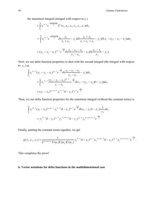
48 Santanu Chakraborty
the innermost integral (integral with respect to x 1)
∞ x1
+ x2
+ x3
α1−1
−
2 *
= ∫ x1
e δ ( x1,
x2
, x3,
y1,
y2
, y3
) dx1
0
= ∫
∞ x1
+ x2
+ x3
α1−1
− x
2
1
x1
+ x2
x1
e δ ( − y1)
δ (
− y2
) δ ( x1
− ( y3
− x2
− x3
)) dx1
x
0
1 + x2
x1
+ x2
+ x3
y
3
−
α1−1
y3
− x2
− x
2
3 y3
− x3
= ( y3
− x2
− x3
) e δ (
− y1)
δ ( − y2
) .
y − x
y
3
Next, we use delta function properties to deal with the second integral (the integral with respect
to x 2 ) as
∞
y3
α −
−
− − −
2 1
α 1 y3
x
2
2 x
1
3
∫ x2
( y3
− x2
− x3
) e δ (
− y1)
dx2
y − x
0
3 3
∞
α1−1
y3
α 1 ( 3 2 3)
2 − y − x − x −
2
∫ x2
e ( x2
− ( y3
− x3
)( 1−
y1))
dx2
y
0
3 − x3
y3
1
−
α1
+ α 2 −1
α1−
α 2 −1
2
( y3
− x3
) y1
( 1−
y1)
e
= δ
=
Then, we use delta function properties for the outermost integral (without the constant terms) is
∞
∫
0
x
y3
α −1
−
−
+ −1
1
−1
1
3 α1
α 2 α1
α 2 2
3 ( y3
− x3
) y1
( 1−
y1)
e δ ( x3
− y3
( 1−
y2
)) dx3
y3
y3
α1
−1
1
1
1
1
−
α 2 − α1+
α 2 −
α3
− α1+
α 2 + α3
− 2
= y1
( 1−
y1)
y2
( 1−
y2
) y3
e
Finally, putting the constant terms together, we get
g(
y1,
y2
, y3
) =
2
1+
α 2 + α3
This completes the proof.
α
1
y
Γ(
α ) Γ(
α ) Γ(
α )
1
2
3
3
α1−1
1
( 1−
y
α 2 −1
α1+
α 2 −1
1)
y2
6. Vector notations for delta functions in the multidimensional case
3
( 1−
y
y3
1
1
−
α3
− α1+
α 2 + α3
− 2
2 ) y3
e
.