5 Graph Description Language (GDL) - Absint

aiSee
Graph Visualization
User Documentation for Windows – Version 2.2.11
AbsInt Angewandte Informatik GmbH
info@AbsInt.com
http://www.AbsInt.com
Release: Version 2.2.11
Date: 21 January 2006
Status: Release
Reference: aiSee-manual-absint
Copyright notice:
c○ 2006 by AbsInt Angewandte Informatik GmbH
All rights reserved. This document, or parts of it, or modified versions of it, may not be copied, reproduced
or transmitted in any form, or by any means, or stored in a retrieval system, or used for any purpose, without
the prior written permission of AbsInt Angewandte Informatik GmbH.
The information contained in this document is subject to change without notice.
LIMITATION OF LIABILITY:
Every effort has been taken in manufacturing the product supplied and drafting the accompanying documentation.
AbsInt Angewandte Informatik GmbH makes no warranty or representation, either expressed or implied,
with respect to the software, including its quality, performance, merchantability, or fitness for a particular
purpose. The entire risk as to the quality and performance of the software lies with the licensee.
Because software is inherently complex and may not be completely free of errors, the Licensee is advised
to verify his work where appropriate. In no event will AbsInt Angewandte Informatik GmbH be liable
for any damages whatsoever including – but not restricted to – lost revenue or profits or other direct,
indirect, special, incidental, cover, or consequential damages arising out of the use of or inability to use
the software, even if advised of the possibility of such damages, except to the extent invariable law, if any,
provides otherwise.
AbsInt Angewandte Informatik GmbH also does not recognize any warranty or update claims unless explicitly
provided for otherwise in a special agreement.

Contents
1 Introduction 9
2 Overview 10
3 Usage 11
3.1 Starting aiSee . . . . . . . . . . . . . . . . . . . . . . . . . . . . . . . . . . . . . 11
3.1.1 Calling aiSee from the Command Line . . . . . . . . . . . . . . . . . . . 11
3.1.2 Starting aiSee . . . . . . . . . . . . . . . . . . . . . . . . . . . . . . . . . 11
3.2 aiSee Window . . . . . . . . . . . . . . . . . . . . . . . . . . . . . . . . . . . . . 11
3.2.1 Graph Window and Virtual Window . . . . . . . . . . . . . . . . . . . . . 11
3.2.2 Message Window . . . . . . . . . . . . . . . . . . . . . . . . . . . . . . . 12
3.2.3 Text Window . . . . . . . . . . . . . . . . . . . . . . . . . . . . . . . . . 12
3.3 Navigating Through a Graph . . . . . . . . . . . . . . . . . . . . . . . . . . . . . 13
3.3.1 Keys . . . . . . . . . . . . . . . . . . . . . . . . . . . . . . . . . . . . . 13
3.3.2 Mouse Pointer . . . . . . . . . . . . . . . . . . . . . . . . . . . . . . . . 13
3.3.3 Scrollbars (Fine-Tuning) . . . . . . . . . . . . . . . . . . . . . . . . . . . 13
3.3.4 Panner Window for Exploring Large Graphs . . . . . . . . . . . . . . . . 13
3.3.5 Following Edges . . . . . . . . . . . . . . . . . . . . . . . . . . . . . . . 14
3.3.6 Follow Edge Dialog Box - History List of Nodes . . . . . . . . . . . . . . 14
3.3.7 Entering Coordinates . . . . . . . . . . . . . . . . . . . . . . . . . . . . . 15
3.3.8 Picking Position . . . . . . . . . . . . . . . . . . . . . . . . . . . . . . . 16
3.3.9 Centering Nodes . . . . . . . . . . . . . . . . . . . . . . . . . . . . . . . 17
3.3.10 Show Neighbors . . . . . . . . . . . . . . . . . . . . . . . . . . . . . . . 17
3.3.11 Scroll Menu . . . . . . . . . . . . . . . . . . . . . . . . . . . . . . . . . . 17
3.4 Scaling the Graph . . . . . . . . . . . . . . . . . . . . . . . . . . . . . . . . . . . 18
3.4.1 Keys . . . . . . . . . . . . . . . . . . . . . . . . . . . . . . . . . . . . . 18
3.4.2 Scale Scrollbar . . . . . . . . . . . . . . . . . . . . . . . . . . . . . . . . 18
3.4.3 Scale Menu . . . . . . . . . . . . . . . . . . . . . . . . . . . . . . . . . . 18
3.5 Node Information . . . . . . . . . . . . . . . . . . . . . . . . . . . . . . . . . . . 18
3.5.1 Application Specific Information . . . . . . . . . . . . . . . . . . . . . . . 19
3.5.2 Node Label . . . . . . . . . . . . . . . . . . . . . . . . . . . . . . . . . . 19
3.5.3 Node Layout Attributes . . . . . . . . . . . . . . . . . . . . . . . . . . . . 19
3.5.4 Statistics of the Graph . . . . . . . . . . . . . . . . . . . . . . . . . . . . 20
3

3.6 Auxiliaries (User Action) . . . . . . . . . . . . . . . . . . . . . . . . . . . . . . . 20
3.7 Ruler . . . . . . . . . . . . . . . . . . . . . . . . . . . . . . . . . . . . . . . . . 20
3.8 File Operations . . . . . . . . . . . . . . . . . . . . . . . . . . . . . . . . . . . . 20
3.8.1 Export Dialog Box . . . . . . . . . . . . . . . . . . . . . . . . . . . . . . 21
3.8.2 File Selector Dialog Box . . . . . . . . . . . . . . . . . . . . . . . . . . . 23
3.9 Exiting aiSee . . . . . . . . . . . . . . . . . . . . . . . . . . . . . . . . . . . . . 23
4 Advanced Usage 24
4.1 Grouping of graph elements . . . . . . . . . . . . . . . . . . . . . . . . . . . . . 24
4.1.1 Grouping of edges . . . . . . . . . . . . . . . . . . . . . . . . . . . . . . 24
4.1.2 Grouping of nodes . . . . . . . . . . . . . . . . . . . . . . . . . . . . . . 24
4.1.3 Example . . . . . . . . . . . . . . . . . . . . . . . . . . . . . . . . . . . 25
4.1.4 Edge Classes - Expose/Hide Edges . . . . . . . . . . . . . . . . . . . . . . 27
4.1.5 Subgraph . . . . . . . . . . . . . . . . . . . . . . . . . . . . . . . . . . . 27
4.1.6 Path Region . . . . . . . . . . . . . . . . . . . . . . . . . . . . . . . . . . 28
4.1.7 Neighbor Region . . . . . . . . . . . . . . . . . . . . . . . . . . . . . . . 28
4.2 Representation of Groups of Nodes . . . . . . . . . . . . . . . . . . . . . . . . . . 29
4.2.1 Folding . . . . . . . . . . . . . . . . . . . . . . . . . . . . . . . . . . . . 29
4.2.2 Box . . . . . . . . . . . . . . . . . . . . . . . . . . . . . . . . . . . . . . 30
4.2.3 Cluster . . . . . . . . . . . . . . . . . . . . . . . . . . . . . . . . . . . . 30
4.2.4 Wrapping . . . . . . . . . . . . . . . . . . . . . . . . . . . . . . . . . . . 31
4.2.5 Displaying Exclusively . . . . . . . . . . . . . . . . . . . . . . . . . . . . 31
4.2.6 Summary Nodes . . . . . . . . . . . . . . . . . . . . . . . . . . . . . . . 32
4.3 Views . . . . . . . . . . . . . . . . . . . . . . . . . . . . . . . . . . . . . . . . . 32
4.3.1 Normal . . . . . . . . . . . . . . . . . . . . . . . . . . . . . . . . . . . . 32
4.3.2 Fish-Eye View . . . . . . . . . . . . . . . . . . . . . . . . . . . . . . . . 33
4.3.3 General Parameters . . . . . . . . . . . . . . . . . . . . . . . . . . . . . . 36
4.4 Changing the Layout . . . . . . . . . . . . . . . . . . . . . . . . . . . . . . . . . 37
4.5 Reducing Layout Time . . . . . . . . . . . . . . . . . . . . . . . . . . . . . . . . 40
5 Graph Description Language (GDL) 42
5.1 Graph Format . . . . . . . . . . . . . . . . . . . . . . . . . . . . . . . . . . . . . 42
5.2 Node Format . . . . . . . . . . . . . . . . . . . . . . . . . . . . . . . . . . . . . 42
5.3 Edge Format . . . . . . . . . . . . . . . . . . . . . . . . . . . . . . . . . . . . . . 43
5.3.1 Ordinary Edge Format . . . . . . . . . . . . . . . . . . . . . . . . . . . . 43
4

5.3.2 Back Edge Format . . . . . . . . . . . . . . . . . . . . . . . . . . . . . . 43
5.3.3 Near Edge Format . . . . . . . . . . . . . . . . . . . . . . . . . . . . . . 44
5.3.4 Bent Near Edge Format . . . . . . . . . . . . . . . . . . . . . . . . . . . 44
5.4 Attribute Format . . . . . . . . . . . . . . . . . . . . . . . . . . . . . . . . . . . 45
5.4.1 Default Node and Edge Attributes . . . . . . . . . . . . . . . . . . . . . . 45
5.4.2 Default Summary Node and Edge Attributes . . . . . . . . . . . . . . . . 46
5.5 Region Format . . . . . . . . . . . . . . . . . . . . . . . . . . . . . . . . . . . . 46
5.6 Examples of GDL Specifications . . . . . . . . . . . . . . . . . . . . . . . . . . . 47
5.6.1 A Cyclic Graph . . . . . . . . . . . . . . . . . . . . . . . . . . . . . . . . 47
5.6.2 Control Flow Graph . . . . . . . . . . . . . . . . . . . . . . . . . . . . . 49
5.6.3 The Effect of the Layout Algorithms . . . . . . . . . . . . . . . . . . . . . 53
5.6.4 Tree Layout . . . . . . . . . . . . . . . . . . . . . . . . . . . . . . . . . . 60
5.6.5 Combination of Features . . . . . . . . . . . . . . . . . . . . . . . . . . . 62
5.7 Graph Attributes . . . . . . . . . . . . . . . . . . . . . . . . . . . . . . . . . . . 66
5.8 Node Attributes . . . . . . . . . . . . . . . . . . . . . . . . . . . . . . . . . . . . 93
5.9 Edge Attributes . . . . . . . . . . . . . . . . . . . . . . . . . . . . . . . . . . . . 100
5.10 Colors . . . . . . . . . . . . . . . . . . . . . . . . . . . . . . . . . . . . . . . . . 105
5.11 Icons and Additional Fonts . . . . . . . . . . . . . . . . . . . . . . . . . . . . . . 106
5.11.1 Icons . . . . . . . . . . . . . . . . . . . . . . . . . . . . . . . . . . . . . 106
5.11.2 Fonts . . . . . . . . . . . . . . . . . . . . . . . . . . . . . . . . . . . . . 106
5.11.3 Compatibility with SVG . . . . . . . . . . . . . . . . . . . . . . . . . . . 107
5.12 User Action . . . . . . . . . . . . . . . . . . . . . . . . . . . . . . . . . . . . . . 109
5.13 Character Set . . . . . . . . . . . . . . . . . . . . . . . . . . . . . . . . . . . . . 109
5.14 Remarks . . . . . . . . . . . . . . . . . . . . . . . . . . . . . . . . . . . . . . . . 111
5.15 GDL’s Grammar . . . . . . . . . . . . . . . . . . . . . . . . . . . . . . . . . . . 112
5.16 Animations . . . . . . . . . . . . . . . . . . . . . . . . . . . . . . . . . . . . . . 114
5.16.1 Animation of layout phases (aka smooth transitions) . . . . . . . . . . . . 114
5.16.2 Animating graph specification sequences . . . . . . . . . . . . . . . . . . 114
6 Overview of the Layout Phases 115
6.1 Parsing . . . . . . . . . . . . . . . . . . . . . . . . . . . . . . . . . . . . . . . . 115
6.2 Grouping of Nodes and Edges – Folding Phase . . . . . . . . . . . . . . . . . . . 115
6.3 Force-Directed Layout . . . . . . . . . . . . . . . . . . . . . . . . . . . . . . . . 115
6.4 Hierarchical Layout . . . . . . . . . . . . . . . . . . . . . . . . . . . . . . . . . . 117
5

6.4.1 Rank Assignment . . . . . . . . . . . . . . . . . . . . . . . . . . . . . . . 117
6.4.2 Crossing Reduction . . . . . . . . . . . . . . . . . . . . . . . . . . . . . . 118
6.4.3 Coordinate Calculation . . . . . . . . . . . . . . . . . . . . . . . . . . . . 119
6.4.4 Edge Bending . . . . . . . . . . . . . . . . . . . . . . . . . . . . . . . . . 120
6.5 Drawing . . . . . . . . . . . . . . . . . . . . . . . . . . . . . . . . . . . . . . . . 120
6.6 Message Characters . . . . . . . . . . . . . . . . . . . . . . . . . . . . . . . . . . 120
7 Tables 121
7.1 Node Attributes Table . . . . . . . . . . . . . . . . . . . . . . . . . . . . . . . . . 121
7.2 Statistics Table . . . . . . . . . . . . . . . . . . . . . . . . . . . . . . . . . . . . 121
7.3 Keyboard Commands Table . . . . . . . . . . . . . . . . . . . . . . . . . . . . . . 121
7.4 Command Line Options . . . . . . . . . . . . . . . . . . . . . . . . . . . . . . . . 124
7.4.1 General Options . . . . . . . . . . . . . . . . . . . . . . . . . . . . . . . 124
7.4.2 General Layout Options . . . . . . . . . . . . . . . . . . . . . . . . . . . 124
7.4.3 Layout Algorithms . . . . . . . . . . . . . . . . . . . . . . . . . . . . . . 126
7.4.4 Layout Speed Options – Iteration Factors . . . . . . . . . . . . . . . . . . 127
7.4.5 View Options . . . . . . . . . . . . . . . . . . . . . . . . . . . . . . . . . 128
7.4.6 Printer Driver Options . . . . . . . . . . . . . . . . . . . . . . . . . . . . 129
7.4.7 Animation Options . . . . . . . . . . . . . . . . . . . . . . . . . . . . . . 132
7.4.8 Windows Option . . . . . . . . . . . . . . . . . . . . . . . . . . . . . . . 133
References 134
Index 136
6

Acknowledgements
aiSee is based on the graph layout tool VCG (Visualization of Compiler Graphs). The work on
VCG started as a diploma thesis written by Iris Lemke at Saarland University in 1991. The goal
was to develop a tool that supports the understanding of the internal data structures of a compiler.
Soon it became clear that such a graph layout tool was very useful in the context of compiler
construction, e.g, for the debugging of compilers. The Department for Programming Languages
and Compiler Construction at Saarland University decided to increase the efforts in the graph
layout area, and VCG was redesigned, widely extended and reimplemented.
The VCG tool won the Graph Visualization Competition in Princeton (in the category “directed
graphs”) in 1994 and in Passau in 1995 (in the category A and honorably mentioned in category B).
The key author of the VCG tool, Dr.-Ing. Georg Sander, received the GI-Dissertationspreis in 1997
(National Award, German Computer Science Society) for his work on “Visualisierungstechniken
für den Compilerbau”.
In January 2000, AbsInt Angewandte Informatik GmbH licensed the non-public version of VCG
from the Saarland University for commercial usage.
Foremost, we would like to thank the key author Dr.-Ing. Georg Sander for the outstanding development.
We would like to thank Iris Lemke, Martin Sicks, Stephan Thesing, Marc Langenbach,
Christian Ferdinand, Judith Engelkamp and Amy S. Bryant who contributed in various stages to
aiSee and/or its documentation, Gerhard Korz and Prof. Dr. Maximilian Herberger who were very
supportive and patient during the license negotiations, Prof. Dr. Reinhard Wilhelm who provided
the environment to develop VCG at his chair at Saarland University, the COMPARE group who
had the pleasure and pain to work with early versions of VCG, and the many VCG users who
provided valuable feedback.

1 Introduction
aiSee is a tool that automatically calculates a customizable layout of graphs specified in GDL
(Graph Description Language). This layout is then displayed, and can be interactively explored,
printed, and exported to various formats.
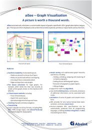
aiSee reads a textual and human-readable graph specification and visualizes the graph. Its design
has been optimized to handle large graphs automatically generated by applications (e. g. compilers).
aiSee was developed to visualize the internal data structures typically found in compilers. Today
it is widely used in many different areas:
• Genealogy (family trees)
• Business management (organization charts)
• Software development (call graphs, control flow graphs)
• Hardware design (circuit diagrams, networks)
• Genetic engineering (complex pedigrees)
• History research (evolution diagrams)
• Informatics (animation of sorting algorithms)
• Database management (entity relationship diagrams)
There are many applications that offer GDL interfaces. Some of them are freely available on the
Internet.
9

2 Overview
The Usage section contains the basics the user needs to know for using aiSee. Upon completing it
the user is able to do the following:
• Navigate through graphs
• Scale them
• Access additional information represented by each node
• Print graphs
The Advanced Usage section describes subgraphs, regions of nodes and different views of the
graph. Subgraphs and regions are used to structure graphs, thereby facilitating interactive exploration
of a graph. Finally, it is explained how layout and view parameters can be changed.
The GDL section is written for programmers who want to produce graph specifications from their
application program which can then be visualized using aiSee.
The Overview of the Layout Phases section provides an introduction to the internals of aiSee and
the underlying graph layout algorithms.
10

3 Usage
This chapter describes the basics of using aiSee.
3.1 Starting aiSee
aiSee can be invoked either from the command line in a window running the MSDOS command
interpreter or like any other Windows program.
3.1.1 Calling aiSee from the Command Line
aiSee can be called with a single file or with a sequence of files.
Single Graph Specification:
Sequence of Graph Specifications:
aisee [options] [filename]
aisee -multi [options_file1] [filename1] [options_file2] [filename2] . . . [options_filen] [filenamen]
After calling aiSee with the -multi flag and a sequence of graph specifications the first graph is
visualized and displayed. To see the next graph in the sequence, choose Next File from the File
menu.
3.1.2 Starting aiSee
aiSee can be started from the Start–>Programs pop up menu, from the Start–> Run menu, or
by double-clicking on the aiSee program icon.
3.2 aiSee Window
The aiSee window consists of a menu line, an optional toolbar, a drawing area (graph window)
with one scrollbar, a text area below the graph window where messages are printed and a status
line.
3.2.1 Graph Window and Virtual Window
aiSee allocates a drawing area called virtual window. Its size is determined by the screen resolution
or the xmax (see p. 91) and ymax (see p. 91) values in the graph specification.
11

Figure 1: aiSee Window
The graph window (display window) shows part of the virtual window. If the graph window is
smaller than the virtual window scrollbars can be used to move the graph window over the virtual
window. This is very useful for precision-positioning the graph window.
3.2.2 Message Window
The message window is used to display short help messages such as explanations of selected menu
items.
3.2.3 Text Window
The text window displays warnings and error messages. Switching between the graph and the text
window is done via the menu item Text Window / Graph Window (Misc menu of the menu
line) or by toggling the Text/Graph Window button on the toolbar.
12

3.3 Navigating Through a Graph
There are several different ways to navigate through a graph.
3.3.1 Keys
The easiest way to explore a graph is by using the arrow keys. The display window is moved 256
pixels in the corresponding direction. Scrolling corresponds to the menu items listed below. They
are located in the Scroll submenu of the Position menu.
Scrolling direction Key Menu item
↑
Scroll upwards ↑ UUp
←
↓
→
Scroll to the left
Scroll to the right
Scroll downwards
←
→
↓
LLeft
RRight
DDown
Go to origin (0,0) o Origin
The o key positions the upper left corner of the display window in the upper left corner of the
graph.
3.3.2 Mouse Pointer
The mouse pointer can be used to scroll the display window through the virtual window:
When the any mouse button is pressed and held, followed by dragging over the graph window, the
graph moves in the direction the mouse pointer was dragged.
3.3.3 Scrollbars (Fine-Tuning)
The vertical and horizontal scrollbars for the display window are used to scroll the display window
through the virtual window. These scrollbars enable the position of the visible part of the graph
to be fine-tuned. The scrollbars are enabled by the Virual Window Scrollbars-swith in the
Misc-menu.
3.3.4 Panner Window for Exploring Large Graphs
Another method of exploring large graphs is to use the panner window (see Figure 2). The main
window shows a magnified view of part of the graph whereas the panner window shows a scaleddown
view of the whole graph. The magnified part of the graph is marked by a rectangle (surrounded
by a dashed line) in the panner window. Dragging this rectangle in the panner window
enables the virtual window to be moved over the graph. The virtual window can be positioned anywhere
by clicking that position in the panner window. To open the panner window, select Panner
from the Scroll menu in the menu line (see Figure 2).
13

3.3.5 Following Edges
Figure 2: Activating the Panner Window
When working with very large graphs where the nodes are connected by long edges it is useful to
navigate through the graph by taking advantage of the graph structure. This is done by following
edges through the graph. The Follow Edge item of the Position menu in the menu line offers
this navigation method; alternative: press the e key.
The Follow Edge operation works like this:
1. One node has to be selected by the mouse.
2. One edge that starts or ends at this node is highlighted.
3. Left-clicking highlights the next edge. Right-clicking centers the node at the other end of
the highlighted edge.
4. From the new node another edge can be selected to be followed by left-clicking.
5. Right-clicking ends the Follow Edge operation.
3.3.6 Follow Edge Dialog Box - History List of Nodes
A history is implemented via the Follow Edge operation so that the path through the graph can be
traced back. Pressing the h key during the Follow Edge operation causes the history dialog box
to appear (see Figure 4) and shows all the nodes encountered during the Follow Edge operation .
The list of nodes is shown as a list of the following node attributes:
• Title (default)
• Label
14

• Information field 1, 2, or 3
The Follow Edge Dialog Box is used as follows:
• Selecting a node from the list and then pressing the Select Node button centers the selected
node in the main window.
• The Next Edge button enables the edges connected to the centered node in the main window
to be cycled through. The next edge to be followed is chosen in this manner.
• Pressing the Follow Edge button causes the edge selected to be followed.
3.3.7 Entering Coordinates
Figure 3: aiSee Follow Edge Navigation
The absolute position of the virtual window can be changed by choosing Position in the Position
menu of the menu line. This causes a dialog box to pop up prompting the user for the absolute
(x,y) coordinates.
15

Figure 4: aiSee Follow Edge Dialog Box
This is followed by the upper left corner of the virtual window and the upper left corner of the
display window being moved to these absolute coordinates.
There are several ways to find out about the values of absolute coordinates.
• Turn on the ruler (see p. 20).
• Invoke Misc–>Information–>Statistics to get information about the maximum size of
the virtual window (Maximum x coordinate and Maximum y coordinate).
• Invoke Misc–>Information–>Node Attributes to find out about the absolute positions
of nodes (see layout attributes on p. 19.
• The absolute coordinates of the mouse pointer position are shown in the status line.
3.3.8 Picking Position
To navigate through the graph using the mouse pointer, choose Pick Position in the Position
menu of the menu line or press the p key.
The Pick Position operation works in two modes:
• New origins can be selected continuously by repeated short left-clicking at any position in
the graph window. With each click the upper left corner of the graph window moves to the
position clicked on in the virtual window. This operation continues until the right mouse
button is pressed.
It is only of limited use for the normal view (see p. 32), however it is especially helpful
for fish-eye view (see p. 33). In fish-eye view the Pick Position operation sets the new
16

focus. The entire graph is drawn in self-adaptable fish-eye view, consequently this operation
enables the entire graph to be easily browsed through by moving the focus over any points
of interest.
• When the left mouse button is pressed and held, followed by dragging over the graph window,
a rubber band appears. This not only causes the origin to be set but also a scaling to be
calculated so that just the area inside the rubber band is magnified to fit in the graph window.
3.3.9 Centering Nodes
Select Center Node... in the Position menu of the menu line or press the n key to open the Title
dialog box. This enables nodes to be continuously chosen which are centered in the main window.
3.3.10 Show Neighbors
Select Show Node in the Position menu of the menu line or press the s key to select a node
to show all its direct neighbors (connected by an visible, invisible or hidden edge) in the graph
specification. Edges can be hidden because egde classes can be hidden (see edge classes on p. 27)
or because of folded or boxed subgraphs (see subgraphes on p. 27).
Each neighbor is annotated by an arrow head in order to distinguisch outgoing edges from incoming
ones. A number in parentheses indicates the class of an edge. Invisible edges are indicated,
too.
3.3.11 Scroll Menu
The submenu of the menu item Scroll of the Position in the menu line offers different ways of
moving the virtual window through the coordinate system.
Menu item Movement of virtual window
Panner Invokes the panner window
Left 32 pixels to the left
Right 32 pixels to the right
Up 32 pixels upwards
Down 32 pixels downwards
LLeft (d) 256 pixels to the left
RRight (c) 256 pixels to the right
UUp (a) 256 upwards
DDown (b) 256 downwards
LLLeft
RRRight One screen size (size of graph window)
UUUp in the corresponding direction
DDDown
Origin Moves to the absolute position (0,0)
17

3.4 Scaling the Graph
If not specified otherwise in the graph specification, aiSee starts with an absolute scale factor of
100% (referred to as “normal”). To scale a graph one of the following three methods can be used.
3.4.1 Keys
The easiest way to scale a graph is by using one of the following keys in the graph window:
3.4.2 Scale Scrollbar
Key Scale factor
= 200 % of the current scale factor
+ 150 % of the current scale factor
− 66 % of the current scale factor
__ 50 % of the current scale factor
0 1 Sets the scale factor to normal (100%).
m Sets the scale factor so that the whole graph is entirely visible.
The second horizontal scrollbar below the graph window is used to set the scale factor of the graph.
If the “thumb” of the scrollbar is in the middle of the scrollbar, scaling is 100 %, i. e. it is normal
size.
3.4.3 Scale Menu
Another way to scale a graph is to use the Scale submenu in the menu line.
Menu item Scale factor
Normal 100 % (absolute)
Maximum Aspect Sets the scale factor so that the whole graph is visible.
x % Skales to x % of the current scale factor
3.5 Node Information
Apart from a node label, additional information, i. e. text can be associated with a node.
The Information submenu in the Misc menu of the menu line enables this information to be
accessed.
• To access the desired information, choose one of the submenu entries or press one of the
keys i, j, or k and left-click on a node.
1 This is the number zero.
18

• Clicking in an open information window causes it to close again.
• Right-clicking enables Show Information to be exited.
3.5.1 Application Specific Information
aiSee allows up to three different pieces of additional information, i.e. text fields, to be associated
with a node. For instance, an application using aiSee to visualize graphs may provide additional
information with each node. Usually the application defines titels for these pieces of information,
enabling the titels to be found and selected in information submenu.
If no titles are defined by the application the default menu items are:
Menu item Key Effect
0 (normal, i) i Information window
1 (normal, j) j is displayed
2 (normal, k) k with a scale factor of normal.
0 (scaled) Information window
1 (scaled) is displayed
2 (scaled) with the current scale factor.
For example, if aiSee is used to visualize family trees in which the nodes contain the names, the
additional information fields could be used to display the date and place of birth and the individual’s
address as shown below.
Example menu items:
3.5.2 Node Label
Menu item
Date of Birth (normal, i)
Place of Birth (normal, j)
Address (normal, k)
Date of Birth (scaled)
Place of Birth (scaled)
Address (scaled)
The menu item Node Label displays the label of a node in normal size. This is useful if the graph
has been reduced to such an extent that label text is no longer readable.
3.5.3 Node Layout Attributes
The Node Layout menu item shows the layout attributes of nodes, such as the node title, a node’s
absolute (x,y) coordinates, width and height, etc. (for the list of attributes shown in the information
window, see table 8 on page 121).
19

3.5.4 Statistics of the Graph
The Statistics menu item shows some statistics pertaining to the graph including the graph size,
number of nodes and edges, number of crossings, etc. (for a list of items shown in the statistics,
see table 9 on page 122).
3.6 Auxiliaries (User Action)
The concept of user actions allows to execute system commands from within aiSee. The Auxilliaries
submenu enables these commands to be accessed. To execute the commands specified in
the GDL specification, choose one of the submenu entries or press one of the keys 1, 2, 3, or 4.
The commands differ in the way that command line arguments are supplied to command:
• User action 1 and 2 take no arguments.
• User action 3 requires one node to be selected as argument.
• User action 4 requires a set of nodes to be selected as arguments.
3.7 Ruler
Selecting Ruler in the Misc menu of the menu line causes the vertical and horizontal rulers at the
margins of the display window to be turned off and on. This can also be done by pressing the r key.
The rulers show the absolute coordinates of the virtual window in the coordinate system. Note:
The ruler does not work for fish-eye views.
3.8 File Operations
All file operations are supported by a file selector dialog box (see p. 23) to select a file name.
The submenu File in the menu line offers the following file operations:
• Open File...
Opens the file selector box (see p. 23) to select a file name. A new graph specification is read
from the file selected, a layout calculated, followed by the graph being displayed.
• Reopen File (g)
This operation causes the file containing the current graph specification to be read again, the
layout recalculated and the graph displayed again. It can also be invoked by pressing the g
key.
• VCG1.0 Save...
Opens the file selector box (see p. 23) to select a file name. The graph currently displayed
is then written to the file selected along with some calculated layout parameters. Note:
This is a legacy feature providing compatibility to VCG V.1.0. It may not work for graph
specifications that contain any newer GDL features.
20

There is no direct interface for printing graphs. However, graphs or parts of graphs can be exported
to files in several formats for which many printer drivers are available. Exporting is done via the
export dialog box (see p. 21).
• Print/Export Part...
A rectangular rubberband is used to select part of the graph currently shown in the display
window. Selecting is done like this:
– Press the left mouse button and hold it down: The rubberband appears.
– Drag it over the area of the graph to be exported followed by releasing the mouse
button.
After selecting the area to be exported the export dialog box (see p. 21) pops up.
Hint: To facilitate selecting the part to be exported it is useful to shrink the graph to a size
so that this part is entirely visible.
Note: It is not possible to export parts of a graph if splines have been used for drawing the
edges.
• Print/Export Graph...
The Export dialog box (see p. 21) is opened.
3.8.1 Export Dialog Box
The export dialog box (see Figure 5) enables the format, scaling, size and position of the exported
image of the graph or part thereof to be selected.
The following export formats are offered:
• PBM: monochromatic PBM-P4 2 format (black and white bitmap format)
• PPM: color PPM-P6 3 format (color bitmap format)
• BMP: bitmap format. BMP format can be either
– monochromatic (black and white) or
– colored.
• PostScript: image description language. The PostScript image can be either
– monochromatic (black and white),
– grey scaled, or
– colored.
2 Portable Bitmap File format
3 Portable Pixmap File format
21

Figure 5: Export Dialog Box
The image can be split into 1, 4, 9, 16, 25, 36 or 49 pages and is surrounded by a bounding
box if the Bounding Box radio button is enabled.
• SVG: scalable vector graphics file format. The image can be either black and white, grey
scaled or colored.
After selecting the format, the orientation and the paper size can be chosen, followed by adjusting
the size and position of the image.
Bitmap formats: The dpi factors of the printer should be selected first because the size depends
on these factors. The x-dpi and y-dpi factors are independent of one other, so that it is possible to
distort the image with these factors.
The Scaling, Width, Height scrollbars can be used to change the size of the image. These three
scrollbars are interconnected, meaning that changing one of them influences the others so as to
preserve the aspect ratio.
The size of the image can also be selected, using the following two shortcut buttons:
• Scaling: 100% causes the image to be exported in normal size (100% absolute).
• Maxspect causes the image to be exported to the chosen paper format in maximum size.
Finally the position of the image on the paper can be chosen using one of the following:
• Center centers on the page, horizontally and vertically
22

• Center width centers horizontally
• Center height centers vertically
Positioning can also be done by moving the small rectangle (with the diagonals) within the panner.
Clicking on the OK button opens the file selection dialog box (see p. 23).
3.8.2 File Selector Dialog Box
Figure 6: File Selector Dialog Box
A file selector dialog box appears for all file operations (see Figure 6).
To switch to a directory or select a file, double-click on the corresponding entry using the left
mouse button.
3.9 Exiting aiSee
aiSee is quit by pressing the q key on the keyboard or by choosing Quit in the File menu.
23

4 Advanced Usage
4.1 Grouping of graph elements
Graphs consist of nodes and edges. aiSee offers various ways of grouping nodes and edges. Grouping
is done either statically, i. e. in the graph specification, or dynamically, i. e. interactively. If not
stated otherwise, the operations mentioned in this section are all located in the Folding menu of
the menu line.
4.1.1 Grouping of edges
A group of edges is a set of edges belonging to the same edge class. The user con expose/hide edges
by enabling/disabling edge classes. Edges of enabled edge classes and target nodes are drawn in
the graph window. Edges of disabled edge classes and all nodes accessible via these edges are not
drawn and are not considered in the layout calculation of the graph.
4.1.2 Grouping of nodes
A group of nodes is either
• A subgraph
• A region specified by paths (path region), or
• A region of neighboring nodes (neighbor regions)
A group of nodes can be treated in a special way. It can be:
• Folded into a summary node,
• Shown in a box,
• Shown as a cluster,
• Wrapped, or
• Represented exclusively.
A summary node is usually drawn in a special shape and/or background color so as to be recognized
as a summary node. It represents all the nodes that are hidden by the folding operation. A summary
node can be:
• unfolded,
• unfolded into a box,
• unfolded and represented as a cluster, or
• unfolded and wrapped.
24

4.1.3 Example
Figure 7 shows a nested graph in different grouping and folding stages. This graph consists of
five subgraphs: Graph A to Graph E. Graph B and C are subgraphs of Graph A. Graph E is a
subgraph of Graph D.
1. All graphs are clustered. In this case it is not possible to choose a different layout for subgraphs.
2. All graphs are boxed. Boxed graphs are drawn in independent frames. Edges between nodes
in different frames are substituted by edges between frames. For example, edge I–>M is
represented by the substitute edge Graph C–>M and edge L–>Graph E is represented by
substitute edge Graph A–>Graph D.
Note: Different layout algorithms or layout parameters can be chosen within boxes. For
example, graph B is drawn in a force-directed layout, graph C in a tree layout with a top
down orientation and graph E right-left-oriented.
3. The frames of graphs B, C, and E are now folded. Nodes inside these frames, i. e. the nodes
of the corresponding subgraphs, disappear.
4. The frames of graphs A and D are unfolded and the formerly substituted edges are shown.
Edge Graph C–>N is represented by the substitute edge Graph C–>Graph E, since N is
a node of the folded graph E.
5. The summary nodes of graphs B, C, and E are unfolded. No frames and summary nodes any
longer exist in this rendering. Therefore edges like Graph E–>N are substituted. Substituted
edges are introduced that start/end at the root node of a frame/subgraph. For example, edge
Graph E–>N is now represented by the substitute edge F–>N since F is the root node of
graph C.
6. Graphs A and D are boxed again, but graphs B, C, and E remain unfolded.
7. Graphs B, C, and E are wrapped. This operation doesn’t change the layout.
25

Figure 7: Several Representations of Groups of Nodes
26

4.1.4 Edge Classes - Expose/Hide Edges
The edges of a graph can be partitioned statically into edge classes by providing an integer for each
edge. Edges with the same integer form a class. These edge class numbers appear in the Select
Edge Classes dialog box. Instead of the numbers the GDL specification can provide names for
edge classes, e. g. if a syntax tree with type information is visualized the edge classes could be
“type edges” and “syntax tree edges”.
After selecting Expose/Hide Edges... in the Folding menu the Select Edge Classes dialog
box appears (see Figure 8). The box shows all the edge classes present.
Edges of enabled edge classes and their target nodes are drawn in the graph window. Edges of
disabled edge classes and all nodes accessible via these edges are not drawn and are not considered
in the layout calculation of the graph.
4.1.5 Subgraph
Figure 8: Edge Class Menu
A graph can be partitioned into nested subgraphs. Subgraphs can be defined only statically, i. e. in
the graph specification. In the GDL specification, subgraphs should be specified in such a manner
so that the user can identify subgraphs and summary nodes and thus make use of all the operations
that work on subgraphs.
Operations: Subgraphs can be
27

• Folded into a summary node (menu item Fold Subgraph),
• Presented in a box (menu item Box Subgraph),
• Represented as a cluster (menu item Cluster Subgraph),
• Wrapped (menu item Wrap/Unwrap Subgraph), or
• Drawn exclusively (menu item Exclusive Subgraph).
Selection: A subgraph is selected by clicking on one of its nodes. The interactive folding, boxing,
clustering and wrapping operations allow more than one subgraphto be selected at the same time.
Instructions appearing in the message window guide the user through the selection procedure.
4.1.6 Path Region
A path region consists of all the nodes making up the paths from a set of start nodes to a set of end
nodes whereby all edges forming the paths have to belong to the edge classes selected.
Operations: A path region can be
• Folded into a summmary node (menu item Fold Region...),
• Presented in a box (menu item Box Region...), or
• Drawn exclusively (menu item Exclusive Region...).
Selection: After one of the region operations is invoked the Select Edge Classes dialog box
appears for selecting the edge classes the region operation is confined to. Then a set of regions has
to be selected. The region operation is then applied to each member of this set.
A single region is selected as follows:
• Select the start nodes by left-clicking on them.
• Now press right mouse button.
• Select the end nodes by left-clicking on them.
To finish selecting an individual region, press the right mouse button.
4.1.7 Neighbor Region
A neighbor region consists of all nodes that are a maximum of n edges away from the start nodes
and belong to the edge classes selected. The direction of the edges is immaterial here.
28

Operations: A neighbor region can be
• Folded into a summary node(menu item Fold Neighbors...),
• Presented in a box (menu item Box Neighbors...), or
• Drawn exclusively (menu item Exclusive Neighbors...).
Selection: After one of the neighbor region operations is invoked the Select Edge Classes dialog
box appears for selecting the edge classes the neighbor region operation is confined to. Then a set
of regions has to be selected. The region operation is then applied to each member of this set.
A single neighbor region is selected by choosing the start nodes by left-clicking on them.
To finish selecting an individual region, press the right mouse button.
To finish selecting the set of regions, press the right mouse button again.
Neighbor Region Range: The number n of edges that defines the size of a neighbor region can
be changed in the View dialog box. Select View... in the Misc menu in the menu line. The number
n (n = 3 by default) appears in the View dialog box below Neighbor Region Range and is changed
by using the scrollbar.
4.2 Representation of Groups of Nodes
A group of nodes (a subgraph, path region or neighbor region) can be
• Folded into a summary node,
• Presented in a box,
• Represented as a cluster,
• Wrapped, or
• Represented exclusively.
4.2.1 Folding
The nodes belonging to a group are hidden. They are represented by a single node called the
summary node. Summary nodes are usually drawn in a different shape and/or color, so that they
can be recognized and selected for the reverse operation.
Targets
The fold operation can be chosen for a
• Subgraph (menu item Fold Subgraph or press the f key),
• Path region (menu item Fold Region...),
29

• Neighbor region (menu item Fold Neighbors...), or
• Box (menu item Fold Box).
Summary nodes
A summary node represents all the nodes of a group that was folded dynamically, i.e. by a folding
operation, or statically, i.e. in the graph specification. A summary node can be selected and
• Unfolded (menu item Unfold/Unbox or press the u key)
• Unfolded into a box (menu item Unfold into Box or x)
• Unfolded and represented as a cluster (menu item Unfold into Cluster or t)
• Unfolded and wrapped (menu item Unfold and Wrap or w)
• Drawn exclusively (menu item Exclusively)
4.2.2 Box
A boxed group of nodes is surrounded by a frame, i. e. drawn in a nested box. The nodes inside
the box are independent of the rest of the graph, i. e. there are no edges connecting nodes outside
of the box with nodes inside the box or vice versa. The layout for the graph inside a box can differ
from the layout of the outer graph.
The layout calculation for graphs with boxes is fast since the nodes inside the box are independent
of the rest of the graph and the layout of the box is calculated separately.
Targets
The box operation can be chosen for a
• Subgraph (menu item Box Subgraph),
• Path region (menu item Box Region...), or
• Neighbor region (menu item Box Neighbors...).
Reverse Operation
The reverse operation is Unfold/Unbox (or press the u key).
4.2.3 Cluster
A clustered group of nodes is surrounded by a frame. In contrast to a box, edges from nodes
outside the frame are drawn to nodes inside the frame and vice versa.
Here the layout is calculated as if the graph were unfolded, the only difference being that the
nodes are placed according to the restrictions induced by the common frame. This often results in
rather poor layout quality, layout calculation frequently being slow on account of the restrictions.
Consequently, the boxed layout is preferable whenever possible.
30

Note: Clustering is an experimental feature. The layout of clustered subgraphs is quite challenging
by nature. aiSee includes an experimental implementation of clustered layout which is
currently not supported nor maintained. Nevertheless, many aiSee users find this feature quite
useful.
Targets
The cluster operation can only be chosen for subgraphs (menu item Cluster Subgraph) or summary
nodes (menu item Unfold into Cluster, or press the t key).
Reverse Operation
A direct reverse operation is not implemented. To reverse a cluster operation, change the clustered
subgraph into a box or fold it and then use Unfold/Unbox.
4.2.4 Wrapping
All nodes and edges belonging to a group are wrapped using the same color. The layout is not
changed.
Note: Nested wrapping is not supported.
Targets
The wrapping operation can only be chosen for subgraphs (Wrap/Unwrap Subgraph).
Reverse Operation
The reverse operation is Wrap/Unwrap Subgraph.
4.2.5 Displaying Exclusively
A group of nodes is shown exclusively. Not all other nodes of the graph are visible. Only edges
between nodes of the group are visible.
Targets
The exclusive displaying of groups of nodes can be chosen for a
• Subgraph (menu item Exclusive Subgraph),
• Path region (menu item Exclusive Region...),
• Neighbor region (menu item Exclusive Neighbors...),
• Box (menu item Exclusive),
• Summary node (menu item Exclusive).
Reverse Operation
The reverse operation is All Subgraphs/Regions.
31

4.2.6 Summary Nodes
A summary node appears after a folding operation. It represents all the nodes grouped by the
folding operation.
Usually summary nodes can be distinguished from normal graph nodes (e. g. they are drawn in a
different shape and/or color) so that they can be recognized as summary nodes. Then they can be
selected and unfolded.
A summary node can be
• Unfolded (menu item Unfold/Unbox or press the u key),
• Unfolded into a box (menu item Unfold into Box or press the x key),
• Unfolded and represented as a cluster (menu item Unfold into Cluster, press the t key),
• Unfolded and wrapped (menu item Unfold and Wrap or press the w key),
• Drawn exclusively (menu item Exclusive).
4.3 Views
A view is how a graph appears in the graph window after the layout is calculated.
There are two main views of a graph:
• Normal view
• Fish-eye view
There are two different kinds of fish-eye views:
– Cartesian fish-eye view (see Figure 10)
– Polar fish-eye view (see Figure 11)
Select View... in the Misc menu in the menu line or press the v key to open the View dialog box
(see Figure 9), in which the different views can be selected and the view parameters changed.
4.3.1 Normal
The graph appears in the graph window, a flat coordinate system being depicted by a linear scale.
The scaling factor for the graph is infinitely variable (see scaling on p. 18). Despite the scaling
possibilities there is often a compromise in the image of large graphs between a detailed view
and an overview. Therefore, the following two browsing methods exist. They can also be used in
combination:
• Information -> Node Label
Displays the label of a node in normal size, very useful if the graph has been scaled down to
such an extent that label text is no longer readable. (see Node Labels p. 19).
32

Figure 9: View Dialog Box
• Scroll -> Panner
The graph is scaled down in a second little window (the panner window), so that the whole
graph is visible. A dashed rectangle marks the part of the graph that is visible in the main
window. (see Panner Window on p. 13).
4.3.2 Fish-Eye View
A common problem of scaling operations is that zooming on a focus often results in losing sight
of important contextual information. That’s why aiSee integrates sophisticated graph distortion
techniques, which imitate the well-known fish-eye lens effect: A focus area is magnified and other
parts of the graph are displayed with less detail. Thus, enabling the user to concentrate on areas of
particular interest while still considering their context.
The graph appears in the graph window, the window depicting a distorted coordinate system, consequently
distorting the image of the graph. The main point of interest is the focus, the focus being
magnified and shown in detail. The parts of the graph that are further away from the focus appear
slightly squashed, meaning the further nodes are positioned away from the focus, the smaller they
appear in the graph window.
Consequently, the relation between the original graph and the visible image of the graph is not
linear, but rather depends on the distance from the focus. This mechanism is similar to the fish-eye
lenses used in photography.
There are four different modes for fish-eye views:
• Self-adaptable fish-eye view (default)
• Fish-eye view with a fixed radius
• Fish-eye with a double focus
• Filtering fish-eye views
The last three items are controlled by parameters (see p. 34).
33

Cartesian Fish-Eye View: Cartesian fish-eye view corresponds to a transformation of the Cartesian
coordinate system.
In a Cartesian view, horizontal and vertical lines are still drawn as parallel horizontal and vertical
lines. Many layouts are based on orthogonal lines. This view improves the readability of such
layouts.
Figure 10: Cartesian Fish-Eye View
Polar Fish-Eye View: Polar fish-eye view corresponds to a transformation of the polar coordinate
system, a transformation in which the plane of a normal coordinate system is projected onto a
sphere. The polar fish-eye view corresponds to a three-dimensional view onto this sphere.
In a polar view, horizontal and vertical lines do not necessarily appear orthogonal.
Browsing through a fish-eye view involves moving the focus. This can be done very easily via
Pick Position (see p. 16) and the other positioning operations (see p. 13) enabling the origin to
be set in a flat view.
Fish-Eye View Modes/Parameters:
34

Figure 11: Polar Fish-Eye View
Self-Adaptable Fish-Eye View: This is the default mode when fish-eye view is activated. Here
the whole graph is visible. The distortion scale of the fish-eye view is automatically adapted to the
current fish-eye view so that the graph just fits in the window.
The position of the focus in the window corresponds to the position of the focus in the graph. This
way the user can extrapolate from the position of the focus in the window to the position of the
focus in the graph. If the focus is positioned in the middle of the graph window this means that
the user is viewing the middle part of the graph. If the focus is closer to e. g. near the upper frame
of the graph window this means that the user is viewing the upper part of the graph. This helps to
maintain orientation when browsing through the graph.
Fish-Eye View with a Fixed Radius: In this mode, the whole graph is not visible but rather only
a fixed radius around the focus.
In this case, the focus is always centered in the graph window.
This view is selected when the fixed radius fish-eye parameter is enabled in the View dialog box.
After enabling this mode the radius of the visible region around the focus can be changed using a
scrollbar (Radius item).
35

Fish-Eye View with a Double-Focus Point: There are two focus in this mode which are created
by overlapping two fish-eye views. The two focus can be positioned independently of one another.
Pick Position (see p. 16) always changes the position of the focus that is closest to the newly
selected position.
The entire graph is visible in this mode. The distortion scale of the two fish eyes is automatically
adapted to the current fish eyes so that the graph just fits in the window.
Note: A double focus is an experimental feature.
Fish-Eye View with a Focal Area: A focal area is possible in lieu of a focal point, the graph not
being distorted inside the focal area. The size of the focal area can be changed via the Size fish-eye
parameter. In polar view the shape of the focal area is a circle and in Cartesian view it is a square.
Filtering Fish-Eye View: A filtering fish eye shows a lot of details around the focus, with details
located far away from the focus being filtered, i. e. only the important objects (nodes and edges)
are actually drawn there and the unimportant ones omitted.
The filtering fish-eye view does not work unless the graph specification indicates the importance
of each node. This factor is indicated by an integer for each node. The higher the number the more
important the node.
This factor enables aiSee to decide whether a node is to be filtered out or drawn. There is a global
parameter called Level (level of detail) that controls how many details are visible in the graph
window. The higher this value the more details are filtered out. A value of zero corresponds to
an unfiltered view of the graph. Level is one of the fish-eye parameters and is found in the View
dialog box.
4.3.3 General Parameters
The View dialog box offers some general view parameters that can be turned on or off providing
the aiSee installation supports this feature:
• Display/hide all edges
• Display/hide all nodes
• Use/do not use splines for drawing edges
• Display/hide icons
• Enable/disable fast font drawing
• Display/hide all node/edge labels
• Display/hide all subgraph labels
In addition, Animation Speed after Relayout can be adjusted or turned off in this box. The speed
is specified in terms of the maximum number of animated iterations. If a new layout is calculated
36

for a graph and if animation is turned on, meaning a rate or animation speed is given, the user can
follow the movement of the nodes from their initial positions in the layout to the newly calculated
ones. The rate or speed refers to the number of animated iterations. (cf. graph attribute amax,
p. 66).
The value of Neighbor Region Range describes the extent of the neighbor region (see p. 28).
4.4 Changing the Layout
The submenu Layout of the Misc menu in the menu lineoffers the following possibilities to
change the layout of the graph:
• Layout...
Changes the layout for an individual graph, i. e. either for an individual subgraph or the
top-level graph only. This operation can also be invoked by pressing the l key.
• Pass Layout...
Changes the layout parameters for the selected graph (subgraph or top-level graph) and then
passes the setting of all the layout parameters of the selected graph to all its subgraphs.
• Pass Changes...
Changes the layout parameters for the selected graph (subgraph or top-level graph) and then
passes only the setting of the changed layout parameters of the selected graph to all its
subgraphs.
After selecting one of these items a boxed subgraph can be chosen for which the layout is to be
changed by left-clicking in the box. Right-clicking causes the layout of the top-level graph to be
changed.
After that the Layout dialog box appears, where the layout parameters can be changed. The layout
parameters take effect when the dialog box is closed by selecting the OK button. This yields a new
layout of the graph. Clicking on Cancel causes the old parameters to remain in effect.
The following layout parameters can be changed:
• Layout Attributes
This section it can be specified whether edge labels are to be drawn, what they look like,
where they are positioned and what the edges are to look like.
– Edge labels (see display_edge_labels on p. 69)
– Dirty labels (see dirty_edge_labels on p. 69)
– Near edges (see near_edges attribute on p. 80)
– Double edges
If this option is disabled doubled edges are not drawn, i. e. if more than one edge exists
between a source node and a target node, only one edge is drawn between these nodes
(see also summarize option on p. 126)
37

Figure 12: Layout Dialog Box
– Fine-tuning (see finetuning on p. 71)
– Splines (see splines on p. 84)
– Manhattan edges (see manhattan_edges on p. 79)
– SManhattan edges (see smanhattan_edges on p. 84)
– priority phase (see priority_phase on p. 81)
– Straight phase (see straight_phase on p. 85)
– Linear segments (see linear_segments on p. 78)
• Orientation
Enables the orientation of the graph in the window to be selected
(see orientation, p. 80).
• Crossing Heuristics
Enables the crossing reduction phases to be controlled.
– The crossing reduction method can be selected
(see crossing_weight on p. 69 ).
– Optimize phase 2 (see crossing_phase2 on p. 69 )
– Optimize local (see crossing_optimization on p. 69 )
• Node Alignment (see p. 80)
38

• Arrow Heads
Enables the mode for the arrow heads to be selected.
– Inport sharing, Outport sharing (see p. 81)
– Fixed arrow heads (see arrow_mode on p. 66)
• Adding Labels (see late_edge_labels on p. 76)
• Layout Factors
Enables all the layout factors to be changed via scrollbars. For example, if the graph is too
dense, X Space and Y Space should be increased; if the splines are too sharp, the spline
factor should be reduced and the XL Space increased.
– Down factor (see layout_downfactor on p. 78 )
– Up factor (see layout_upfactor on p. 78 )
– Near factor (see layout_nearfactor on p. 78 )
– X Base (see xbase on p. 91 )
– Y Base (see ybase on p. 91 )
– X Space (see xspace on p. 92 )
– Y Space (see yspace on p. 92 )
– XL Space (see xlspace on p. 92 )
– Spline factor (see splinefactor on p. 84 )
This factor can only be changed if splines are used for edge drawing.
– Time limit
Enables a time limit for layout calculation to be set. If the time limit is exceeded, the
fastest possible mode for the current iteration phase is activated.
• Maximum Iteration Factors
Enables the maximum iteration factors for the various layout calculation phases to be
changed.
– Crossingred. (see cmax on p. 68 )
– Medium Shifts (see pmax on p. 80 )
This factor cannot be changed for the tree layout.
– Center Shifts (see rmax on p. 82 )
This factor cannot be changed for tree layout.
– Spread Level (see spreadlevel on p. 84 )
This factor can only be changed for tree layout.
– Tree Factor (see treefactor on p. 88 )
This factor can only be changed for tree layout.
– Straight Line (see smax on p. 84 )
– Bending Reduction (see bmax on p. 67 )
39

• Minimum Iteration Factors
Enables the minimum iteration factors for the various layout calculation phases to be
changed.
– Crossing Reduction (see cmin on p. 68 )
– Medium Shifts (see pmin on p. 80 )
– Center Shifts (see rmin on p. 82 )
• Layout Speed
Enables the layout calculation speed to be controlled via appropriate iteration factor settings.
In fact these buttons are shortcuts for changing the iteration factors Crossing Reduction,
Medium Shifts, Center Shifts, Straight Line and Bending Reduction all at once.
• Partitioning Algorithm
When it comes to hierarchical layout algorithms, the order in which the nodes are visited
influences the layout greatly. The following algorithms are available:
– Normal (see p. 76)
– Dfs (see p. 76) )
– Maxdepth (see p. 76) , mindepth (see p. 76)
– Maxdepthslow (see p. 76) , mindepthslow (see p. 76)
– Maxindegree (see p. 77) , minindegree (see p. 77)
– Maxoutdegree (see p. 77) , minoutdegree (see p. 77)
– Maxdegree (see p. 77) , mindegree (see p. 77)
– Minbackward (see p. 77)
– Tree layout (see p. 77)
4.5 Reducing Layout Time
aiSee was designed to explore large graphs. However, the layout of large graphs may require
considerable time. Thus, there are many possibilities to speed up the layout algorithm: The graph
can be folded, iterations can be limited, and time limits can be specified.
The first step in visualizing a large graph is avoiding computing the layout of parts of the graph that
are currently not of interest. These parts should be specified as initially folded in the specification.
Folding makes the visible part of the graph smaller, thus enabling the layout to be calculated faster
and the quality of the layout improved. It is useful to first try one of the fast algorithms (dfs,
minbackward, tree), then the medium fast methods (normal, mindepth, maxdepth, ...) before
resorting to the slower methods (mindepthslow, maxdepthslow).
In order to further reduce layout time, some layout phases should be omitted or the maximum
number of iterations of some layout phases limited. However, this usually decreases the quality of
the layout. First, the crossing reduction phase 2 (option -nocopt2, attribute crossing_phase2)
should be skipped as it usually takes the most time. Crossing reduction phase 2 is indicated by
40

B in the message window (see p. 120). Next, the iterations for the crossing reduction can be
limited (-cmax option, cmax attribute) or another crossing weight selected (-bary option, etc.,
crossing_weight attribute). Normally, it is not necessary to switch off local crossing optimization,
because this step is quite fast and effective.
If the graph is very unbalanced, the pendulum method may require considerable time (indicated by
m in the message window). In this case, the number of iterations for the crossing reduction should
be limited (-pmax option, pmax attribute). If the straight-line fine-tuning phase takes too long
(indicated by S in the message window), its maximum iteration number should be limited (-smax
option, smax attribute).
Other parameters usually needn’t be changed, because the corresponding phases are quite fast.
Bending reduction in particular improves layout quality greatly and is so fast that the -bending
option is hardly needed.
Fast mode (-fast option) drastically reduces all iteration limits and may result in poor layout
quality.
The drawing of splines is slow, consequently it should be avoided on large graphs.
It is also possible to set a time limit (-timelimit option). If the time limit is exceeded, the
fastest possible mode for the current and the following iteration phases is selected. Selecting a
time limit does not mean that the layout has actually finished when the time has elapsed: Layout
may be faster if the graph is small and/or its structure is simple. It may be much slower, because
even the fastest possible methods may take some time. The time limit is real time, thus the result
of the layout may depend on the load of the computer. Thus, given a time limit, two identical trials
needn’t result in identical layouts.
41

5 Graph Description Language (GDL)
GDL is an ASCII text representation of a graph. It describes a graph in terms of nodes, edges,
subgraphs and attributes. A subgraph is described as a normal graph except that it is specified inside
another graph, meaning graph specifications can be nested. aiSee provides special operations for
subgraphs such as folding (see p. 29) to a summary node (see p. 32) , boxing (see p. 30) , clustering
(see p. 30) , or wrapping (see p. 31) .
Graphs, nodes and edges may have attributes that specify details of their appearance on the screen
such as colors, sizes, shapes etc.
There is always only one top-level graph.
It is also possible to specify regions that are to be initially folded after starting aiSee.
aiSee also accepts the #line directives of the C preprocessor. The macro processing facilities of
the C preprocessor offers some tricky possibilities for graph specifications. For example, using a
macro directive would enable different languages for node labels to be chosen.
5.1 Graph Format
A graph (the top-level graph or a subgraph) is specified by
graph: {
< list of graph_entries >
}
A graph_entry is one of the following:
• subgraph (see p. 42) , i. e. a subgraph is specified in the same manner a top-level graph is
specified. There is no special keyword for subgraphs.
• node (see p. 42)
• edge (see p. 43)
• attribute (see p. 45)
• region (see p. 46)
The delimiter between items of a list is one or more whitespace characters (spaces, tabs, line feeds,
carriage returns). There is no order required for nodes, edges, subgraphs, or attributes. However,
depending on the layout algorithm selected, the order of nodes may influence the layout.
5.2 Node Format
A node is specified by
node: {
title: < node title >
42

}
< list of node attributes >
The title of a node is any valid C string. Strings have to be enclosed in quotes and may contain the
normal C escapes (e. g. \", \n, \f, . . . ).
5.3 Edge Format
There are several different kinds of edges:
• ordinary edges (see p. 43)
• back edges (see p. 43)
• near edges (see p. 44)
• left near edges (see p. 44)
• right near edges (see p. 44)
• bent near edges (see p. 44)
• left bent near edges (see p. 45)
• right bent near edges (see p. 45)
5.3.1 Ordinary Edge Format
An ordinary edge is specified by
edge: {
source: < title of source node >
target: < title of target node >
< list of edge attributes >
}
5.3.2 Back Edge Format
Back edges are drawn in the opposite direction as compared to ordinary edges. For instance, if the
layout algorithm tries to give all ordinary edges a top-down orientation, it tries to give the back
edges a bottom-up orientation.
If a graph contains a cycle, not all edges can have the same orientation: Some edges have to be
reversed. In this case, the layout algorithm prefers back edges before selecting any other edge to
be reversed.
A back edge is specified by
backedge: {
source: < title of source node >
43

}
target: < title of target node >
< list of edge attributes >
5.3.3 Near Edge Format
Near edges are drawn so that their source and target nodes are directly neighbored at the same
level. This implies that a node cannot have more than two near edges, i.e. one on the left and one
on the right with respect to the orientation of the graph. Near edges are drawn as short horizontal
lines not crossed by any other edges or nodes.
Hint: Invisible near edges can be used to group nodes at one level.
A near edge is specified by
nearedge: {
source: < title of source node >
target: < title of target node >
< list of edge attributes >
}
Left Near Edge Format: Same as near edge, only that the target node is placed directly neighbored
to the left of the source node at the same level.
leftnearedge: {
source: < title of source node >
target: < title of target node >
< list of edge attributes >
}
Right Near Edge Format: Same as near edge, only that the target node is placed directly neighbored
to the right of the source node at the same level.
rightnearedge: {
source: < title of source node >
target: < title of target node >
< list of edge attributes >
}
5.3.4 Bent Near Edge Format
Bent near edges consist of a horizontal part (same as near edges), a bend point and a vertical part.
An edge label (if any) is placed only at the bend point. So bent near edges connect nodes across
one or more levels yet leave the source node at the left or right side.
A near edge is specified by
bentnearedge: {
source: < title of source node >
44

}
target: < title of target node >
< list of edge attributes >
Left Bent Near Edge Format: Same as bent near edge, only that the horizontal part of the edge
leaves the source node on the left.
leftbentnearedge: {
source: < title of source node >
target: < title of target node >
< list of edge attributes >
}
Right Bent Near Edge Format: Same as bent near edge, only that the horizontal part of the
edge leaves the source node on the right.
rightbentnearedge: {
source: < title of source node >
target: < title of target node >
< list of edge attributes >
}
5.4 Attribute Format
Attributes are specified as follows:
< attribute keyword > : < attribute value >
All attributes are optional except for the title attribute of nodes and the source and target
attribute of edges. The order of attributes is irrelevant.
The attribute value depends on the attribute and is one of the following:
• String, e. g. title: "My family tree"
• Integer, e. g. width: 700
• Floating point number, e. g. scaling: 1.2
• Keyword, e. g. shape: rhomb
• Combination of the above, e.g. fontname: "helvB10"
• File name, e.g. iconfile: "myicons/butterfly.ppm"
5.4.1 Default Node and Edge Attributes
It is possible to specify default values for all node or edge attributes in a top-level graph or subgraph.
The default attributes are specified as follows:
45

• node.< attribute keyword > : < attribute value >
• edge.< attribute keyword > : < attribute value >
These default specifications can appear anywhere in a top-level graph or subgraph specification
and apply to all nodes and edges (including back edges, near edges and bent near edges) respectively
where the corresponding attribute is not set explicitly. This default specification applies
until another default specification for the same attribute appears or until the end of the subgraph or
top-level graph specification is reached.
5.4.2 Default Summary Node and Edge Attributes
Regions of nodes and edges can be folded (see p. 24). As a result, a summary node is displayed for
all nodes of a region of nodes. In addition, summary edges to this summary node are displayed for
sets of edges to nodes of the region. It is possible to specify the attributes for these summary nodes
and edges that come from a folding operation. This allows folded regions to be given a different
appearance than normal nodes and edges. The attributes for these summary nodes or replacement
edges are specified as follows:
• foldnode.< attribute keyword > : < attribute value >
• foldedge.< attribute keyword > : < attribute value >
5.5 Region Format
It is not only possible to fold regions dynamically, i. e. interactively with the mouse, but also
statically, i. e. in the specification of the graph.
The format of a region specification is:
region: {
state: < state of the region (folded, boxed, exclusive) >
source: < list of strings specifying start nodes >
target: < list of strings specifying end nodes >
class: < list of integers specifying edge classes >
range: < integer specifying the neighbor region range >
}
The delimiter between items of a list is one or more whitespace characters. The attributes target,
class and range are optional.
range is used to specify a neighbor region, in which case it gives the maximum number of edges
to be followed in order to reach all the nodes of the neighbor region (see p. 28).
A region cannot have a range and target nodes specified at the same time.
46

5.6 Examples of GDL Specifications
5.6.1 A Cyclic Graph
These examples show a number of small cyclic graphs without any labels but with different edge
types. The titles are displayed in the nodes. The last example in this sequence shows how the
anchor edge attribute is used.
The layout of the following three example specifications are shown in Figure 13.
Example 1: Ordinary Edges
aiSee tries to give all edges the same orientation. But since the graph is cyclic, one edge has to be
reverted (edge D–>A).
01 graph: {
02 // list of nodes
03 node: { title: "A" }
04 node: { title: "B" }
05 node: { title: "C" }
06 note: { title: "D" }
07 node: { title: "E" }
08 // list of edges
09 edge: { source: "A" target: "B" }
10 edge: { source: "A" target: "C" }
11 edge: { source: "C" target: "D" }
12 edge: { source: "D" target: "E" }
13 edge: { source: "D" target: "A" }
14 }
Example 2: Back Edge
The edge to be reverted can be specified as a back edge.
11 backedge: { thickness: 3 source: "C" target: "D" }
Example 3: Near Edges
Near edges can be used to express a close relationship between two nodes and to place nodes rightor
left-neighbored.
09 nearedge: { source: "A" target: "B" }
10 nearedge: { source: "A" target: "C" }
12 nearedge: { source: "D" target: "E" }
The layout of the following three example specifications are shown in Figure 14.
Example 4: Bent Near Edge
In some situations, edges are to be horizontally anchored, like near edges, yet the target node is
not to be at the same level. These edges have to have a bend point. This is why bent near edges are
used.
09 bentnearedge: { source: "A" target: "B" }
47

Figure 13: Ordinary, Back and Near Edges
12 bentnearedge: { source: "D" target: "E" }
Example 5: Right-Bent Near Edge
The left or right versions of bent near edges or near edges can be used if it is important to have
edges anchored to a particular side of a node.
09 rightbentnearedge: { source: "A" target: "B" }
10 leftnearedge: { source: "A" target: "C" }
12 rightnearedge: { source: "D" target: "E" }
Example 6: Anchor
The anchor edge attribute can be used if a node label consists of one or more fields that are on
separate lines where outgoing edges are to start. For example, if node D represents a struct with
two fields whose first field is to point to node E and the second one to node A, then the edges are
anchored to the corresponding anchor points 1 and 2. Counting of anchor points starts with 1 at
the top of a node and increases from top to bottom.
Anchor points and near edge specifications cannot be used together, consequently the specification
for Example 6 looks like this:
01 graph: {
02 // list of nodes
03 node: { title: "A" }
04 node: { title: "B" }
05 node: { title: "C" }
06 node: { title: "D" label: "Field1\nField2" }
07 node: { title: "E" }
08 // list of edges
48

Figure 14: Bent Near, Right-Bent Near and Anchor Edges
09 bentnearedge: { source: "A" target: "B" }
10 nearedge: { source: "A" target: "C" }
11 backedge: { source: "C" target: "D" }
12 edge: { source: "D" target: "E" anchor: 1}
13 edge: { source: "D" target: "A" anchor: 2}
14 }
5.6.2 Control Flow Graph
The following three graphs show the control flow graph of a procedural program. The nodes
contain the text of statements as labels. Not all edges have labels. The visualized control flow
comes from the following nonsense program, which consists of a procedure test and a main
routine in a pseudo imperative language.
PROCEDURE test( VAR b : INTEGER; c : INTEGER );
BEGIN
b := c + 5;
END
BEGIN // main routine of a nonsense program
x := 1;
WHILE (x = 1) DO
x := 2;
test ( x, 1 );
x := 3;
OD;
WHILE (x = 1) DO
x := 4;
x := 5;
test ( x, 2 );
49

OD;
WHILE (x = 1) DO
x := 6;
IF (x = 7) THEN x := 8; ELSE test ( x, 3 );
FI;
OD;
END.
Example 7: Control Flow Graph 1
This example shows a simple visualization of the control flow graph. The graph is shown in
Figure 15.
01 graph: { title: "CFG_GRAPH"
02 splines: yes
03 layoutalgorithm: dfs
04 finetuning: no
05 display_edge_labels: yes
Figure 15: Control Flow Graph 1 – Simple Version
50

06 yspace: 55
07 node: { title:"18" label: "test_b := test_c+5" }
08 node: { title:"17" label: "Exit" }
09 node: { title:"16" label: "test (x,3)" }
10 node: { title:"15" label: "x := 8" }
11 node: { title:"14" label: "x=7" }
12 node: { title:"13" label: "x := 6" }
13 node: { title:"12" label: "x=1" }
14 node: { title:"11" label: "test (x,2)" }
15 node: { title:"10" label: "x := 5" }
16 node: { title:"9" label: "x := 4" }
17 node: { title:"8" label: "x=1" }
18 node: { title:"7" label: "x := 3" }
19 node: { title:"6" label: "test (x,1)" }
20 node: { title:"5" label: "x := 2" }
21 node: { title:"4" label: "x=1" }
22 node: { title:"3" label: "x := 1" }
23 node: { title:"2" label: "Start" }
24 node: { title:"1" label: "Exit point\ntest" }
25 node: { title:"0" label: "Entry point\ntest" }
26 edge: { source:"18" target:"1" }
27 edge: { source:"0" target:"18" }
28 edge: { source:"12" target:"17" label: "false" }
29 edge: { source:"8" target:"12" label: "false" }
30 edge: { source:"16" target:"12" label: "back" }
31 edge: { source:"15" target:"12" label: "back" }
32 edge: { source:"13" target:"14" }
33 edge: { source:"14" target:"16" label: "false" }
34 edge: { source:"14" target:"15" label: "true" }
35 edge: { source:"12" target:"13" label: "true" }
36 edge: { source:"4" target:"8" label: "false" }
37 edge: { source:"11" target:"8" label: "back" }
38 edge: { source:"10" target:"11" }
39 edge: { source:"9" target:"10" }
40 edge: { source:"8" target:"9" label: "true" }
41 edge: { source:"3" target:"4" }
42 edge: { source:"7" target:"4" label: "back" }
43 edge: { source:"6" target:"7" }
44 edge: { source:"5" target:"6" }
45 edge: { source:"4" target:"5" label: "true" }
46 edge: { source:"2" target:"3" }
47 }
Example 8: Control Flow Graph 2
This example shows an improved visualization of the control flow graph. The graph is shown in
Figure 16. The start, exit and branch nodes are drawn in different shapes so that they can be better
51

ecognized. The edges closing a cycle are specified as back edges in order to see the uniform flow
of control in the other edges. The edges at the branch nodes are anchored at the left and right via
the bent near edge specification.
Figure 16: Control Flow Graph 2 with Rhomb-shaped Nodes and Near Edges
01 graph: { title: "CFG_GRAPH"
02 layoutalgorithm: dfs
03 finetuning: no
04 display_edge_labels: yes
05 yspace: 55
06 node: { title:"18" label: "test_b := test_c+5" }
07 node: { title:"17" label: "Exit" shape: ellipse }
08 node: { title:"16" label: "test (x,3)" }
09 node: { title:"15" label: "x := 8" }
10 node: { title:"14" label: "x=7" shape: rhomb }
11 node: { title:"13" label: "x := 6" }
12 node: { title:"12" label: "x=1" shape: rhomb }
13 node: { title:"11" label: "test (x,2)" }
14 node: { title:"10" label: "x := 5" }
15 node: { title:"9" label: "x := 4" }
16 node: { title:"8" label: "x=1" shape: rhomb }
17 node: { title:"7" label: "x := 3" }
18 node: { title:"6" label: "test (x,1)" }
19 node: { title:"5" label: "x := 2" }
20 node: { title:"4" label: "x=1" shape: rhomb }
21 node: { title:"3" label: "x := 1" }
52

22 node: { title:"2" label: "Start" shape: ellipse }
23 node: { title:"1" label: "Exit point\ntest" shape: ellipse }
24 node: { title:"0" label: "Entry point\ntest" shape: ellipse }
25 edge: { source:"18" target:"1" }
26 edge: { source:"0" target:"18" }
27 bentnearedge: { source:"12" target:"17" label: "false" }
28 bentnearedge: { source:"8" target:"12" label: "false" }
29 backedge: { source:"16" target:"12" label: "back" }
30 backedge: { source:"15" target:"12" label: "back" }
31 edge: { source:"13" target:"14" }
32 bentnearedge: { source:"14" target:"16" label: "false" }
33 bentnearedge: { source:"14" target:"15" label: "true" }
34 bentnearedge: { source:"12" target:"13" label: "true" }
35 bentnearedge: { source:"4" target:"8" label: "false" }
36 backedge: { source:"11" target:"8" label: "back" }
37 edge: { source:"10" target:"11" }
38 edge: { source:"9" target:"10" }
39 bentnearedge: { source:"8" target:"9" label: "true" }
40 edge: { source:"3" target:"4" }
41 backedge: { source:"7" target:"4" label: "back" }
42 edge: { source:"6" target:"7" }
43 edge: { source:"5" target:"6" }
44 bentnearedge: { source:"4" target:"5" label: "true" }
45 edge: { source:"2" target:"3" }
46 }
Example 9: Control Flow Graph 3
This example shows another improved visualization of the control flow graph of Example 7. The
graph is shown in Figure 17. Here an orthogonal layout is used so that the graph looks like a
typical flowchart. For orthogonal layout, a large down factor and near factor and an up factor of
zero is recommended. This improves the layout of long vertical edges. Add the following lines to
Example 8 after line 01:
manhattan_edges: yes
layout_downfactor: 100
layout_upfactor: 0
layout_nearfactor: 0
xlspace: 12
5.6.3 The Effect of the Layout Algorithms
The following sequence of layouts shows the same graph visualized by different layout algorithms.
The graph is cyclic, so the algorithm tree can’t be used.
A key problem is selecting the nodes that appear at the top level of the graph. The layout algorithm
looks for candidates that have no incoming edges yet at least one outgoing edge. If such nodes do
53

Figure 17: Control Flow Graph 3 with Manhattan Edges
not exist as in this example (Example 10), the algorithms mindegree, minindegree, maxoutdegree
are the most appropriate algorithms.
The fine-tuning phase eliminates long edges, meaning the tuned graph is more compact. Note that
the tuned graph created by maxdephtslow need not be of maximum depth because fine-tuning may
have reduced the depth further. The tuned graph created by mindepthslow needn’t be of minimum
depth, either. All these partitioning algorithms are heuristics.
Example 10: A cyclic graph
01 graph: {
02 xspace: 25 xlspace: 15
03 node: { title: "0" label: "Start" }
04 node: { title: "1" } node: { title: "2" } node: { title: "3" }
05 node: { title: "4" } node: { title: "5" } node: { title: "6" }
06 node: { title: "7" } node: { title: "8" } node: { title: "9" }
07 node: { title: "0" }
08 edge: { source: "0" target: "1" }
09 edge: { source: "0" target: "2" }
10 edge: { source: "0" target: "3" }
54

11 edge: { source: "0" target: "4" }
12 edge: { source: "0" target: "5" }
13 edge: { source: "0" target: "9" }
14 edge: { source: "1" target: "3" }
15 edge: { source: "2" target: "4" }
16 edge: { source: "3" target: "5" }
17 edge: { source: "5" target: "0" }
18 edge: { source: "9" target: "0" }
19 edge: { source: "0" target: "6" }
20 edge: { source: "6" target: "7" }
21 edge: { source: "7" target: "8" }
22 edge: { source: "8" target: "0" }
23 }
Here follows a discussion of all the different hierarchical layout algorithms with and without finetuning
for this example.
• normal, finetuning: no
The normal layout algorithm breaks the cycle so that only one reverted edge is necessary
(see left of Figure 18).
• normal, finetuning: yes
Compared to the previous layout, the fine-tuning phase has balanced the position of the node
9. The long edge 8–>Start is not balanced since this would create additional reverted edges
(see right of Figure 18).
Figure 18: Example 10, normal layout, with and without finetuning
• dfs, finetuning: no
The layout algorithms dfs, mindepth, minindegree, maxoutdegree and maxdegree happen to
result in the same layout (see left of Figure 19).
• dfs, finetuning: yes
The algorithms dfs, mindepth, minindegree, maxoutdegree and maxdegree happen to result
in the same layout (see right of Figure 19).
55

Figure 19: Example 10, dfs layout, with and without finetuning
• minbackward, finetuning: no
This is almost the same layout as for the normal layout algorithm. Again only one reverted
edge is necessary. The layout algorithm maxdepth without fine-tuning results in the same
layout (see left of Figure 20).
• minbackward, finetuning: yes
Compared to the layout without fine-tuning, here the long edge 8–>Start is partially eliminated
and the position of node 9 is balanced again (see right of Figure 20).
Figure 20: Example 10, minbackward layout, with and without finetuning
• maxdepth, finetuning: no
Same as minbackward without fine-tuning (see left of Figure 20).
• maxdepth, finetuning: yes
The long edge 8–>Start is now fully eliminated. Here, the fine-tuning phase is allowed to
revert additional edges (see left of Figure 21).
• mindepth, finetuning: no
The layout algorithms dfs, mindepth, minindegree, maxoutdegree and maxdegree happen to
result in the same layout (see left of Figure 19).
56

Figure 21: Example 10, maxdepth; and mindegree layout with finetuning
• mindepth, finetuning: yes
Compared to the previous layout the long edge 8–>Start is eliminated. The algorithms dfs,
mindepth, minindegree, maxoutdegree and maxdegree happen to result in the same layout
(see right of Figure 19).
• maxdepthslow, finetuning: no
This depth six layout is in fact of maximum depth as compared to all the other variants (see
left of Figure 22).
• maxdepthslow, finetuning: yes
The fine-tuning phase eliminates the long edge Start–>6. Thus, the layout is no longer of
maximum depth. Fine-tuning may destroy the maximum depth property (see right of Figure
22).
Figure 22: Example 10, maxdepthslow layout, with and without finetuning
• mindepthslow, finetuning: no
Graphs that are of minimum depth tend to have many nodes at the top level. Compared to
57

all untuned graphs, this layout is of minimum depth. It should be noted, however, that the
algorithm mindepth with fine-tuning is able to produce a flatter layout (see left of Figure 23).
• mindepthslow, finetuning: yes
Compared to the previous layout, the long edge 8–>Start is balanced again (see right of
Figure 23).
Figure 23: Example 10, mindepthslow layout, with and without finetuning
• maxindegree, finetuning: no
Here node 3 is placed at the level zero because it has the maximum indegree. Node 0 is not
chosen for level zero because it doesn’t have any outgoing edges (see left of Figure 24).
• maxindegree, finetuning: yes
Once again the long edge 8–>Start of the previous algorithm is eliminated by balancing the
position of node 8. The algorithms dfs, mindepth and minindegree happen to result in the
same layout (see right of Figure 24).
Figure 24: Example 10, maxindegree layout, with and without finetuning
• minindegree, finetuning: no
The layout algorithms dfs, mindepth, minindegree, maxoutdegree and maxdegree happen to
result in the same layout (see left of Figure 19).
• minindegree, finetuning: yes
The algorithms dfs, mindepth, minindegree, maxoutdegree and maxdegree happen to result
in the same layout (see right of Figure 19).
58

• maxoutdegree, finetuning: no
The layout algorithms dfs, mindepth, minindegree, maxoutdegree and maxdegree happen to
result in the same layout (see left of Figure 19).
• maxoutdegree, finetuning: yes
The algorithms dfs, mindepth, minindegree, maxoutdegree and maxdegree happen to result
in the same layout (see right of Figure 19).
• minoutdegree, finetuning: no
Nodes 4 and 0 with a minimum outdegree of zero cannot be start nodes because start nodes
have to have at least one successor otherwise they would create single-node components of
the spanning tree. Start nodes can be any other nodes except Start, from which 1, 2, and 6
happen to be selected (see left of Figure 25).
• minoutdegree, finetuning: yes
The long edges Start–>1, Start–>2 and Start–>6 are eliminated (see right of Figure 25).
Figure 25: Example 10, minoutdegree layout, with and without finetuning
• maxdegree, finetuning: no
The Start node has the maximum number of incoming and outgoing edges, so it is selected as
the start node of the spanning tree, i. e. it appears at the topmost level. The layout algorithms
dfs, mindepth, minindegree, maxoutdegree and maxdegree happen to result in the same
layout (see left of Figure 19).
• maxdegree, finetuning: yes
Compared to the previous layout the long edge 8–>Start is eliminated. The algorithms dfs,
mindepth, minindegree, maxoutdegree and maxdegree happen to result in the same layout
(see right of Figure 19).
• mindegree, finetuning: no
The candidates for start nodes of the spanning tree are 1, 2, 6, 7, 8 and 9 because they have
a minimum degree of two. 1, 2 and 6 happen to be selected as the start nodes. Note that
nodes 4 and 0 are not candidates for start nodes because they do not have outgoing edges.
59

The layout algorithms minoutdegree and mindegree happen to result in the same layout (see
left of Figure 25).
• mindegree, finetuning: yes
Compared to the previous layout, the long edges Start–>1 Start–>2 and Start–>6 are
eliminated. This changes the structure of the layout entirely (see right of Figure 21).
5.6.4 Tree Layout
The following example shows a typed syntax tree. This tree can either be drawn by the specialized
algorithm for “downward laid-out trees” or by the normal algorithms. When the normal algorithms
are used to draw a tree, it is advisable to increase the layout down factor in order to obtain good
results (see Figure 26). If the layout down factor is not used, the incoming edges draw the nodes
too much in the direction of the parent node.
Figure 26: Example 11, normal layout
A nice layout is achieved by the specialized tree algorithm with a tree factor of 0.9 (see Figure 27).
If an orthogonal layout is needed, the attribute smanhattan_edges can be used. For trees, this attribute
is more appropriate than the standard Manhattan layout with manhattan_edges (see Figure
28).
60

Figure 27: Example 11, tree layout, treefactor: 0.9
Example 11: Syntax Tree
01 graph: {
02 title: "Typed Syntax Tree"
03 node: { title:"503160" label: "Identifier\ntst3 (0)" }
04 node: { title:"503240" label: "Identifier\nx (0)" }
05 node: { title:"502952" label: "INTEGER" }
06 node: { title:"503304" label: "VarDecl" }
...
29 node: { title:"T0" label: "no type" }
30 node: { title:"T1" label: "no type" }
31 node: { title:"T2" label: "int" }
...
57 edge: { source:"503304" target:"503240" }
58 edge: { source:"503304" target:"502952" }
...
83 nearedge: { source:"503160" target:"T0" linestyle: dotted }
84 nearedge: { source:"503240" target:"T1" linestyle: dotted }
85 nearedge: { source:"502952" target:"T2" linestyle: dotted }
...
110 }
61

5.6.5 Combination of Features
Figure 28: Example 11, tree layout, smanhattan_edges: yes
The following example (see Figure 29) is taken from [GKNV93] and shows the dependencies of
different shell programs. A combination of aiSee features has been used to visualize it. There is
a time scale to indicate the origin of the programs. The shells themselves are nodes that have to
be placed at the same rank as their birth dates. The level attribute is used to set the nodes at these
positions. In addition, the time axis should be positioned at the left side of the shell dependence
graph. This is achieved by the horizontal_order attribute at some of the nodes. However, this
attribute doesn’t work unless the graph is connected, which is why three invisible edges are created.
Like any other edges, invisible edges influence the positions of the nodes. They pull their adjacent
nodes together. To avoid this effect on the invisible edges, the priority of the invisible edges is set to
zero and the priority of the visible edges to 100. There are many ways to change the priority. The
priority attribute can be set, and the factors layout_downfactor, layout_downfactor and layout_downfactor
as well. The real priority of a downward edge is the product layout_downfactor
x priority.
The Bourne shell should be positioned to the left of the Mashey shell and the csh shell to the
right of the Mashey shell. Therefore, the level two nodes receive a horizontal order. However, csh
is on level three, and only its edge crosses level two. Therefore, the horizontal_order attribute is
set for this edge as well. Now the edge is drawn to the right of the Mashey shell.
Default attribute specifications are used for the height, width and border width of nodes and for
62

the style of edges in order to reduce the amount of specification. The various shell types are
differentiated by using ellipses for the variations of the Korn shell, triangles for C shells and a
rhomb for the tcl shell. The graph is acyclic, which is why the layout algorithm minbackward is
used. Edges are drawn by splines.
Example 12: Development of Shells
01 graph: {
02 title: "shells"
03 splines: yes
04 layoutalgorithm: minbackward
05 layout_nearfactor: 0
06 layout_downfactor: 100
07 layout_upfactor: 100
Figure 29: Development of Shells
63

08
09 // First the time scale
10
11 node.height: 26
12 node.width: 60
13 node.borderwidth: 0
14 edge.linestyle: dashed
15
16 node: { title: "1972" level: 1 horizontal_order: 1}
17 node: { title: "1976" level: 2 horizontal_order: 1 }
18 node: { title: "1978" level: 3 }
19 node: { title: "1980" level: 4 }
20 node: { title: "1982" level: 5 horizontal_order: 1 }
21 node: { title: "1984" level: 6 }
22 node: { title: "1986" level: 7 }
23 node: { title: "1988" level: 8 }
24 node: { title: "1990" level: 9 }
25 node: { title: "future" level: 10 horizontal_order: 1 }
26
27 edge: { source: "1972" target: "1976" }
28 edge: { source: "1976" target: "1978" }
29 edge: { source: "1978" target: "1980" }
30 edge: { source: "1980" target: "1982" }
31 edge: { source: "1982" target: "1984" }
32 edge: { source: "1984" target: "1986" }
33 edge: { source: "1986" target: "1988" }
34 edge: { source: "1988" target: "1990" }
35 edge: { source: "1990" target: "future" }
36
37 // We need some invisible edge to make the graph fully connected.
38 // Otherwise, the horizontal_order attribute would not work.
39
40 edge: { source: "ksh-i" target: "Perl" linestyle: invisible priority: 0 }
41 edge: { source: "tcsh" target: "tcl" linestyle: invisible priority: 0 }
42 nearedge: { source: "1988" target: "rc" linestyle: invisible }
43 nearedge: { source: "rc" target: "Perl" linestyle: invisible }
44
45 // Now the shells themselves
46 // Note: the default value -1 means: no default
47
48 node.height: -1
49 node.width: -1
50 node.borderwidth: 2
51 edge.linestyle: solid
52
53 node: { title: "Thompson" level: 1 horizontal_order: 2 }
54 node: { title: "Mashey" level: 2 horizontal_order: 3 }
55 node: { title: "Bourne" level: 2 horizontal_order: 2 }
56 node: { title: "Formshell" level: 3 }
57 node: { title: "csh" level: 3 shape: triangle }
58 node: { title: "esh" level: 4 horizontal_order: 2 }
59 node: { title: "vsh" level: 4 }
60 node: { title: "ksh" level: 5 horizontal_order: 3 shape: ellipse }
61 node: { title: "System V" level: 5 horizontal_order: 5 }
62 node: { title: "v9sh" level: 6 }
64

63 node: { title: "tcsh" level: 6 shape: triangle }
64 node: { title: "ksh-i" level: 7 shape: ellipse }
65 node: { title: "KornShell" level: 8 shape: ellipse }
66 node: { title: "Perl" level: 8 }
67 node: { title: "rc" level: 8 }
68 node: { title: "tcl" level: 9 shape: rhomb }
69 node: { title: "Bash" level: 9 }
70 node: { title: "POSIX" level: 10 horizontal_order: 3 }
71 node: { title: "ksh-POSIX" level: 10 horizontal_order: 2 shape: ellipse }
72
73 edge: { source: "Thompson" target: "Mashey" }
74 edge: { source: "Thompson" target: "Bourne" }
75 edge: { source: "Thompson" target: "csh" horizontal_order: 4 }
76 edge: { source: "Bourne" target: "ksh" }
77 edge: { source: "Bourne" target: "esh" }
78 edge: { source: "Bourne" target: "vsh" }
79 edge: { source: "Bourne" target: "System-V" }
80 edge: { source: "Bourne" target: "v9sh" }
81 edge: { source: "Bourne" target: "Formshell" }
82 edge: { source: "Bourne" target: "Bash" }
83 edge: { source: "csh" target: "tcsh" }
84 edge: { source: "csh" target: "ksh" }
85 edge: { source: "Formshell" target: "ksh" horizontal_order: 4 }
86 edge: { source: "esh" target: "ksh" }
87 edge: { source: "vsh" target: "ksh" }
88 edge: { source: "ksh" target: "ksh-i" }
89 edge: { source: "System-V" target: "POSIX" }
90 edge: { source: "v9sh" target: "rc" }
91 edge: { source: "ksh-i" target: "KornShell" }
92 edge: { source: "ksh-i" target: "Bash" }
93 edge: { source: "KornShell" target: "Bash" }
94 edge: { source: "KornShell" target: "POSIX" }
95 edge: { source: "KornShell" target: "ksh-POSIX" }
96 }
65

5.7 Graph Attributes
This section describes the whole list of graph attributes. Each attribute is listed together with its
type, default value and where it can be used, i. e. in the top-level graph, a subgraph specification
or in both.
• amax
Type: integer
Default value: automatic
Attribute of: top-level graph
Description:
This attribute specifies the number of iterations that are animated after relayout. Specifying
0 means animation is turned off. This value can be changed interactively in the View dialog
box (see p. 36).
• arrow_mode
Type: fixed, free
Default value: free
Attribute of: top-level graph, subgraphs
Description:
This attribute specifies two modes for drawing arrow heads.
– fixed
This arrow mode should be used if port sharing (see port_sharing on p. 81 ) is used
because then only a fixed set of rotations for the arrow heads are used. Here the arrow
head is rotated only in increments of 45 degrees, and only one arrow head occurs at
each port.
– free
Here each arrow head is rotated individually for each edge. If a node has many incoming
edges, this parameter can lead to a confusing image.
• attraction
Type: integer
Default value: 60
Attribute of: top-level graph
Description:
This attribute applies only to the forcedir layout algorithm.
Here it is part of the force-directed spring embedder during attractive impulse calculation. It
specifies the constant proportional to the attractive forces acting on a node.
This constant and its repulsive counterpart (see p. 82) enable the length of edges to be controlled.
For example, if only attractive and repulsive forces are working on a node, an edge
length of n pixels is achieved for edges with priority of 1 (see edge attribute priority on
p. 103) by specifying n 2 for the attributes attraction and repulsion. Usually the values for
these two attributes are of the same order of magnitude.
For details, see p. 115.
66

• bmax
Type: integer
Default value: 100
Attribute of: top-level graph, subgraphs
Description:
This attribute sets the maximum number of iterations of the phase reducing edge bends.
Edge bends are used to prevent edges from being drawn across nodes. Reducing the number
of iterations reduces layout calculation time, however the layout quality may suffer.
• border
Type:
x : integer pixels or
y : integer pixels
Default value: x : 600, y : 600
Attribute of: top-level graph
Description:
This attribute applies only to the forcedir layout algorithm.
Depending on the specification of the layout parameters for the forcedir layout algorithm it is
possible for nodes to move far away from one another (especially single nodes not connected
to the main graph) This prevents nodes from being placed “infinitely” far from one another.
These two attributes enable a rectangle to be specified within which the graph is drawn.
For details, see p. 115.
• bordercolor
Type: black, blue, red, ...
Default value:
Same as the value of the textcolor attribute for summary nodes
Attribute of: subgraphs
Description:
Specifies the color for borders of summary nodes, boxes and frames of clusters. For details
on colors, see p. 105. See also color (p. 68) and textcolor attribute (p. 87).
• borderstyle
Type: continuous, dashed, dotted, double, invisible, solid, triple
Default value: continuous
Attribute of: subgraphs
Description:
This attribute specifies the line style used for drawing the borders of a summary node. See
also edge attribute linestyle (p. 102).
• borderwidth
Type: integer
Default value: 2 pixels
Attribute of: subgraphs
Description:
This attribute specifies the thickness of the border of a summary node in pixels.
67

• classname
Type: integer : string
Default value: 1 : “1”, 2 : “2”, 3 : “3”, ...
Attribute of: top-level graph
Description:
This attribute enables the names of edges classes to be introduced. These names appear in
the Select Edge Classes dialog box. For details on edge classes, see p. 27.
• cmin, cmax
Type: integer
Default value: 0 for cmin, infinite for cmax
Attribute of: top-level graph, subgraphs
Description:
The cmin attribute sets the minimum number of iterations that are performed for reducing
crossings using crossing weights. The normal method stops when two consecutive checks
no longer cause the number of crossings to be reduced. However, this number of crossings
might be a local minimum, meaning the number of crossing might decrease even more after
some more iterations.
The cmax attribute sets the maximum number of iterations of the crossing reduction phase.
A reduction of this value causes the layout process to be speeded up. The default value
infinite means that the method is iterated as long as any improvement is possible.
• color
Type: black, blue, red, ...
Default value:
white for top-level graph
white for subgraphs
Attribute of: top-level graph, subgraphs
Description:
– top-level graph
Here the color attribute specifies the background color of the graph window.
– subgraphs
Here it specifies the background color of subgraphs. This color is valid as the background
color in summary nodes, boxes, clusters and as a wrapping color.
For details on colors, see p. 105. See also attributes textcolor (p. 87) and bordercolor
(p. 67).
• colorentry
Type: integer : integer integer integer
Default value: no default value defined
Attribute of: top-level graph, subgraphs
Description:
This attribute enables the default color map to be filled and changed. A color is a triple of
integer values for the red, green and blue part. Each integer ranges from 0 (color part turned
off) to 255 (color part turned on), e. g. 0 0 0 specifies the color black and 255 255 255
68

specifies the color white. For instance, colorentry 75 : 70 130 180 sets map
entry 75 to steel blue. This color can be used by merely specifying 75 wherever a color
value is expected. For more details on colors, see p. 105.
• crossing_optimization
Type: yes, no
Default value: yes
Attribute of: top-level graph, subgraphs
Description:
yes activates the crossing optimization phase, which works locally. It is a postprocessing
phase after normal crossing reduction. It tries to optimize locally by exchanging pairs of
nodes to reduce the number of crossings.
• crossing_phase2
Type: yes, no
Default value: yes
Attribute of: top-level graph, subgraphs
Description:
yes activates crossing reduction phase two. In this phase, nodes having equal crossing
weights are permuted. Note that this is the most time-consuming phase of crossing reduction.
• crossing_weight
Type: bary, median, barymedian, medianbary
Default value: bary
Attribute of: top-level graph, subgraphs
Description:
This attribute specifies the weight to be used for crossing reduction. There is no general recommendation
as to which is the best method. A guideline might be to use bary if the degree
of the nodes is large and median or one of the hybrid methods barymedian or medianbary if
the degree is small, the degree of a node being the total of incoming and outgoing edges at a
node. See p. 118 for details.
– bary
The barycenter is used for calculating the weights during crossing reduction. This is
the fastest method for graphs with nodes whose average degree is very large.
– median
The median center is used for calculating the weights during crossing reduction.
– barymedian
These weights are the combination of barycenter and mediancenter weights, with
barycenter having priority and mediancenter only being used for nodes whose barycenter
weights are equal.
– medianbary
These weights are the combination of barycenter and mediancenter weights, with the
mediancenter having priority.
• dirty_edge_labels
Type: yes, no
69

Default value: no
Attribute of: top-level graph, subgraphs
Description:
yes forces a fast layout of edge labels, which may result in overlapping of labels. Dirty edge
labels cannot be used if splines are used for edge drawing.
• display_edge_labels
Type: yes, no
Default value: no
Attribute of: top-level graph, subgraphs
Description:
yes: edge labels are displayed, no: edge labels are not displayed.
• edges
Type: yes, no
Default value: yes
Attribute of: top-level graph
Description:
no: suppresses the drawing of edges in the top-level graph and in all nested subgraphs.
• energetic
Type: yes, no
Default value: no
Attribute of: top-level graph
Description:
This attribute applies only to the forcedir layout algorithm.
Apart from the forces of the spring embedder and the magnetic fields, the local energy level
of a node can be taken into account in deciding whether the node should move or not. Setting
this attribute to yes causes the local energy present at a node to be considered during layout.
For details, see p. 115.
• energetic attraction, energetic repulsion, energetic gravity,
energetic crossing, energetic overlapping, energetic border
Type: float
Default values: see list below
Attribute of: top-level graph
Description:
This attribute applies only to the forcedir layout algorithm.
Apart from the forces of the spring embedder and the magnetic fields, the local energy level
of a node can be taken into account in deciding whether the node should move or not. The
behavior of the local energy present at a node can be influenced via the following attributes:
– energetic attraction, Default value: 70.0
Weight of the attractive energy of edges
– energetic repulsion, Default value: 70.0
Weight of the repulsive energy between nodes
70

– energetic gravity, Default value: 0.3
Weight of the gravitational energy of a node
– energetic crossing, Default value: 80.0
Weight of the global energy of an edge crossing
– energetic overlapping, Default value: 80.0
Weight of the global energy of a node overlapping
– energetic border, Default value: 70.0
Weight of the border energy of a node
Gauging layout quality can be done as follows: The better the layout, the lower the total of
all the energy values mentioned above.
For details, see p. 115.
• equal_y_dist
Type: yes, no
Default value: no
Attribute of: top-level graph, subgraphs
Description:
If this attribute is enabled (yes), then the vertical distance in a hierarchical layout is equal
among all levels.
• fast_icons
Type: yes, no
Default value: no
Attribute of: top-level graph
Description:
yes: causes icon file loading to be faster, which may negatively impact the quality of the
drawing if not all the icon colors are present. For details on pictures in nodes, see p. 106.
• fdmax
Type: integer
Default value: 300
Attribute of: top-level graph
Description:
This attribute only applies to the forcedir layout algorithm.
Here it is used in the simulated annealing part of the algorithm. It specifies the upper hard
limit for the number of iterations performed. The algorithm stops when the global temperature
drops below a threshold value or when the limit specified here is reached.
For details, see p. 115.
• finetuning
Type: yes, no
Default value: yes
Attribute of: top-level graph, subgraphs
Description:
71

no: switches off the fine-tuning phase of the graph layout algorithm. The fine-tuning phase
tries to give all edges the same length. It tries to improve the ranks of nodes in order to avoid
very long edges (see p. 117).
• focus
Type: no type
Default value: no value
Attribute of: subgraphs
Description:
This attribute sets the focus for the summary node of a subgraph, i. e. if the status of the
subgraph is folded at startup, then the summary node of the subgraph for which focus was
specified is centered in the graph window.
Note: The focus can also be specified for nodes (see node attribute p. 93). It goes without
saying that the focus attribute should appear only once in a graph specification.
• fontname
Type: string
Default value: default font drawn by turtle graphics routines
Attribute of: subgraphs
Description:
This attribute specifies a pixel font different from the default font and used for drawing
the text labels of summary nodes. This font is given by the name of the aiSee font file
containing the font description, e.g. a 12-point Times Roman font can be specified via
fontname: "timR12". Note: If the font file is not in the current directory the environment
variable AISEEFONTS has to be set to the directory containing the font description
files. For details on fonts, see p. 106.
• fstraight_phase
Type: yes, no
Default value: no
Attribute of: top-level graph
Description:
yes: forces straight edges that are not anchored at the same position on the border of the
nodes. This is useful only if no port sharing (see p. 81) is selected, because bends are
avoided by correcting the port position.
• gravity
Type: float
Default value: 0.0625
Attribute of: top-level graph
Description:
This attribute only applies to the forcedir layout algorithm.
It is used for impulse calculation. Only using a simulation of a spring embedder would force
unconnected components of a graph to move further and further apart from one another, as
there would be no attractive forces acting between them. That is why gravity is introduced
as a counterforce.
72

This attribute specifies the constant which is proportional to the gravitational force acting on
a node. This constant controls the strength of the gravitational force, e. g. a value of zero
cancels out the influence of any gravitational force.
For details, see p. 115.
• height
Type: integer
Default value:
Top-level graph: (height of root screen - 100) pixels
Subgraphs: (height of the label for summary nodes) pixels
Attribute of: top-level graph, subgraphs
Description:
The meaning of this attribute depends on where it is specified:
– top-level graph
This attribute specifies the height of the display window in pixels.
– subgraphs
Here it specifies the height of the summary node.
See also graph attribute width (p. 90).
• hidden
Type: integer
Default value: none
Attribute of: top-level graph
Description:
This attribute specifies the edge class to be hidden. To hide more than one edge class, repeat
this attribute for each additional edge class. For more details, see p. 27.
Edges in such a class are ignored during layout calculation and are not drawn. Nodes that are
only accessible (forward or backward) via edges of a hidden class are not drawn. However,
nodes that are not accessible at all are drawn (see p. 74).
Note the difference between hiding edge classes and the edge line style invisible (see p. 103).
Hidden edges do not exist in the layout. Edges with the invisible line style exist in the layout,
i. e. they influence the layout, meaning they need space and may produce crossings, for
example.
• horizontal_order
Type: integer
Default value: none (corresponds to -1)
Attribute of: subgraphs
Description:
In a hierarchical layout, this attribute specifies the horizontal position of the summary node
within a level (see p. 89). The nodes specified via horizontal positions are ordered according
to these positions within the levels. Nodes without this attribute are inserted into this ordering
by the crossing reduction mechanism (see p. 118).
73

Note: Connected components are handled separately during crossing reduction, thus it is not
possible to intermix nodes of different connected components in one ordering sequence. For
example, one connected component consists of nodes A, B, C and another of nodes D, E, all
nodes being positioned at the same level. Thus, for instance, it is not possible to specify the
following horizontal order at level 0: A, D, C, E.
Note further: If the algorithm for downward laid-out trees is used the specified horizontal order
is retained only within nodes that are children of the same node, i. e. in case of downward
laid-out trees it is not possible to specify a horizontal order for the entire level.
• iconcolors
Type: integer
Default value: 32
Attribute of: top-level graph
Description:
This attribute specifies the size of the color map used for colors in bitmap files. For details
on pictures in nodes, see p. 106.
• iconfile
Type: string
Default value: no default value
Attribute of: subgraphs
Description:
This attribute specifies the bitmap file (format raw PBM, PPM) to be displayed in the summary
node of the folded subgraph. Note: if the bitmap file to be displayed is not in the current
directory the environment variable AISEEICONS can be set to the directory containing the
bitmap file. For details on pictures in nodes, see p. 106.
• icons
Type: yes, no
Default value: yes
Attribute of: top-level graph
Description:
no: disables displaying of icons in nodes. Displaying of icons can be enabled again interactively
from the View dialog box.
• ignore_singles
Type: yes, no
Default value: no
Attribute of: top-level graph, subgraphs
Description:
yes: hides all nodes of the remaining graph which would appear singly and unconnected.
These nodes have no edges at all and drawing them sometimes results in an ugly layout of
the remaining graph. The default setting is to show all nodes (no option).
• importance
Type: integer
Default value: 0 (which means infinity)
74

Attribute of: subgraphs
Description:
This is the central attribute when it comes to filtering in fish-eye views as it enables the
importance of a summary node of a folded subgraph to be specified via an integer.
Low integers signify less important nodes which are filtered out first by a filtering fish-eye
view. High integer numbers signify nodes that are important, their being rarely filtered out.
A value of 0 represents an infinite importance, the result being that these nodes are never
filtered out. This attribute exists for nodes too, see p. 95.
• info1, info2, info3
Type: string
Default value: empty string for all three
Attribute of: subgraphs
Description:
These attributes enable three additional text fields to be specified for a summary node of a
folded subgraph. The same set of attributes exists for nodes (see node attribute info1, p. 95).
These additional information fields can be selected interactively from the submenu of the
Information menu (see p. 19).
• infoname
Type: integer : string
Default value: 1 : “0”, 2 : “1”, 3 : “2”
Attribute of: top-level graph
Description:
This attribute enables names for the additional information fields available for each node to
be introduced. These names appear in the submenu of the menu item Information in the
Misc menu of the menu line. For details on additional information fields, see p. 19 and p. 75.
• inport_sharing
Type: yes, no
Default value: no
Attribute of: top-level graph, subgraphs
Description
See graph attribute port_sharing (p. 81).
• label
Type: string
Default value: empty string
Attribute of: subgraphs
Description:
This string is displayed inside the summary node of a folded subgraph. If no label is spezified
the value of the title of the subgraph is used. If there is no label or title specified for the
subgraph then the file name of the graph spezification is used.
Note: This text may contain control characters, e.g. “\n” (newline character), that influence
the size of the node (see 5.13)
75

• invisible
Type: integer
Default value: no default value
Attribute of: top-level graph
Description:
This attribute is a synonym for the graph attribute hidden (p. 73).
• late_edge_labels
Type: yes, no
Default value: no
Attribute of: top-level graph, subgraphs
Description:
This attribute controls the moment when edge labels are drawn.
– yes
The graph is first partitioned and then edge labels are introduced.
– no
In this case the algorithm first creates labels and then partitions the graph. This option
yields a more compact layout, but may result in more crossings.
• layoutalgorithm
Type: normal, maxdepth, mindepth, ...
Default value: normal
Attribute of: top-level graph, subgraphs
Description:
This attribute specifies the basic layout algorithms, there being two main categories. The first
fourteen algorithms describe variations of a hierarchical layout, whereas the last algorithm
implements a force-directed layout. The variations differ in the way nodes are selected for
the various levels in the hierarchical layout.
– normal
This algorithm is the default algorithm. It tries to give all edges the same orientation
and is based on the calculation of strongly connected components. The algorithms
based on depth first search are faster.
– dfs
This algorithm uses a depth first search for layout calculation, but does not enforce
additional constraints pertaining to the degree of nodes. It is faster than the normal
layout algorithm. The result is heavily dependent on the initial order of the nodes in
the specification.
– maxdepth/mindepth
These two algorithms are based on depth first search and are both fast heuristics.
maxdepth tries to increase the depth of the layout. mindepth tries to increase the width
of the layout.
– maxdepthslow/mindepthslow
These slower algorithms might be better if the fast heuristics offered by the algorithms
76

maxdepth and maxdepth do not provide satisfying results. maxdepthslow tries to increase
the depth of the layout and mindepthslow the width of the layout.
– maxindegree / minindegree
maxindegree schedules nodes with a maximum of incoming edges first, i. e. these
nodes are positioned early. minindegree schedules nodes with a minimum of incoming
edges first.
– maxoutdegree / minoutdegree
maxoutdegree schedules nodes with a maximum of outgoing edges first, i. e. these
nodes are positioned early. minoutdegree schedules nodes with a minimum of outgoing
edges first.
– maxdegree / mindegree
maxoutdegree schedules nodes with a maximum of the sum of incoming and outgoing
edges first, i. e. these nodes are positioned early. The algorithm minoutdegree schedules
nodes with the minimum of the sum of incoming and outgoing edges first.
– minbackward
Instead of calculating strongly connected components, minbackward performs a topological
sorting to assign ranks to the nodes. This algorithm is fast if the graph is acyclic.
– tree
The tree algorithm is a specialized method for downward laid out (see p. 117). It is
very fast for these tree-like graphs and results in a balanced layout.
– forcedir
This layout algorithm computes a force-directed placement. It is a nonhierarchical
layout method that works well for undirected graphs. Some features of hierarchical
layout like near edges are disabled for this layout algorithm.
The layout calculation for this algorithm can be controlled via the following graph
attributes:
∗ Spring embedder forces
attraction (p. 66), repulsion (p. 82)
∗ Gravitational forces
gravity (p. 72)
∗ Simulated annealing
fdmax (p. 71),
tempmin, tempmax (p. 86),
temptreshold (p. 87), tempscheme (p. 87), tempfactor (p. 86)
∗ Random influence
randomfactor (p. 81), randomrounds (p. 82), randomimpulse (p. 82)
∗ Magnetic forces
magnetic_field1, magnetic_field2 (p. 79),
magnetic_force1, magnetic_force2 (p. 79)
∗ Energy level
energetic (p. 70)
77

energetic attraction (p. 70), energetic repulsion (p. 70)
energetic gravity (p. 70), energetic crossing (p. 70)
energetic overlapping (p. 70), energetic border (p. 70)
∗ Boundary rectangle
border x (p. 67), border y (p. 67)
• layout_downfactor, layout_upfactor, layout_nearfactor
Type: integer
Default value: 1 for all three attributes
Attribute of: top-level graph, subgraphs
Description:
The layout algorithm partitions the set of edges into edges pointing upward, edges pointing
downward, and edges pointing sidewards. The last type of edges is also called near edges.
These attributes have no effect if the layout algorithm tree is used.
If the layout_downfactor is large as compared to the layout_upfactor and layout_nearfactor,
then the positions of the nodes are mainly determined by the edges pointing
downwards.
If the layout_upfactor is large as compared to the layout_downfactor and layout_nearfactor,
then the positions of the nodes are mainly determined by the edges pointing
upwards.
If the layout_nearfactor is large, then the positions of the nodes are mainly determined by
the edges pointing sidewards.
• level
Type: integer
Default value: none (corresponds to -1)
Attribute of: subgraphs
Description:
This attribute is a synonym for vertical_order (p. 89).
• linear_segments
Type: yes, no
Default value: no
Attribute of: top-level graph, subgraphs
Description:
yes switches linear segment layout on. This layout favors straight long vertical edges. See
also -linseg options (p. 125) and -linsegmax (p. 125)
• loc
Type: { x: y: }
Default value:
Top-level graph: { x:0 y:0 } for both
Subgraphs: unspecified for both
Attribute of: top-level graph, subgraphs
Description:
For details, see x (p. 90).
78

• magnetic_field1, magnetic_field2
Type:
no, top_to_bottom, bottom_to_top, left_to_right, right_to_left,
polar, circular, orthogonal, polcircular
Default value: no
Attribute of: top-level graph
Description:
This attribute only applies to the forcedir layout algorithm.
Magnetic fields are part of impulse calculation. Forces that originate from a simulation of a
spring embedder neglect the directions of edges. In directed graphs edges should point in a
uniform direction, consequently magnetic forces are introduced, with edges being interpreted
as magnetic needles that align according to a magnetic field.
Two independent magnetic fields are possible. These two attributes specify the kind of magnetic
field for each. If two fields are specified, the edges are influenced by both. The attributes
magnetic_force1 and magnetic_force2 (p. 79) influence the strength of each field.
For details, see p. 115.
• magnetic_force1, magnetic_force2
Type: integer
Default value: 1 for both
Attribute of: top-level graph
Description:
This attribute only applies to the forcedir layout algorithm.
These two attributes specify the constant factors that are multiplied by the corresponding
magnetic forces of the two magnetic fields.
See also magnetic_field1 and magnetic_field2 (p. 79).
For details, see p. 115.
• manhattan_edges
Type: yes, no
Default value: no
Attribute of: top-level graph, subgraphs
Description:
yes switches orthogonal layout on. Orthogonal layout (or Manhattan layout) means that all
edges consist of horizontal or vertical line segments. Vertical edge segments might be shared
by several edges, while horizontal edge segments are never shared. This results in aesthetic
layouts for flowcharts. If orthogonal layout is used, the priority phase and straight phase are
also used by default (see priorty_phase, p. 81 and straight_phase, p. 85).
• margin
Type: integer
Default value: 0 if the value of borderwidth (p. 67) is zero, 3 otherwise
Attribute of: subgraphs
Description:
79

Specifies the horizontal and vertical offset between the border of a summary node and its
label in pixels. Useful for rectangular nodes only.
• near_edges
Type: yes, no
Default value: yes
Attribute of: top-level graph, subgraphs
Description:
no: All near edges are treated as normal edges in the graph layout.
• nodes
Type: yes, no
Default value: yes
Attribute of: top-level graph
Description:
no: Suppresses the drawing of nodes in the top-level graph and all nested subgraphs.
• node_alignment
Type: top, center, bottom
Default value: center
Attribute of: top-level graph, subgraphs
Description:
For hierarchical layout this attribute specifies the vertical alignment of nodes at the horizontal
reference line of levels.
– top: The tops of all nodes of a level have the same y coordinate.
– center: All nodes of a level are centered.
– bottom: The bottoms of all nodes of a level have the same y coordinate.
• orientation
Type: top_to_bottom, bottom_to_top, left_to_right, right_to_left
Default value: top_to_bottom
Attribute of: top-level graph, subgraphs
Description:
This attribute specifies the orientation of the graph. All explanations in this section are given
in relation to the default orientation.
• outport-sharing
Type: yes, no
Default value: no
Attribute of: top-level graph, subgraphs
Description:
See graph attribute port-sharing (p. 81).
• pmin, pmax
Type: integer
Default value:
80

0 for pmin
100 for pmax
Attribute of: top-level graph, subgraphs
Description:
pmin sets the minimum number of iterations of the pendulum method. Like crossing reduction,
this method stops when the “imbalance weight” stops decreasing. However, an increase
in imbalance weight might be a local phenomenon, meaning that the imbalance might decrease
much more after a few more iterations.
pmax sets the maximum number of iterations of the pendulum method. Reducing this factor
increases layout calculation speed.
• port_sharing, inport_sharing, outport_sharing
Type: yes, no
Default value:
no (since aiSee 2.1.89) for port-sharing,
no for inport-sharing and outport-sharing
Attribute of: top-level graph, subgraphs
Description:
no suppresses the sharing of ports by edges at nodes. inport-sharing enables the port sharing
of incoming edges only, with outport-sharing enabling the port sharing of outgoing edges
only.
Generally speaking, if multiple edges are adjacent to the same node, and the arrow heads of
all these edges have the same appearance (color, size, etc.), these edges may share a port at a
node. This means that only one arrow head is drawn, and all edges meet at this arrow head.
This enables many edges to be located adjacent to one node without getting confused by too
many arrow heads. If no port sharing is used, each edge gets its own port.
• priority_phase
Type: yes, no
Default value: no
Attribute of: top-level graph, subgraphs
Description:
yes switches on the priority phase. This phase replaces the normal pendulum method with
a specialized method: It forces long vertical edges to be straight, just like the straight phase
(see p. 85). In fact, the straight phase is a fine-tuning of the priority phase, the priority phase
being recommended for an orthogonal layout (see manhattan_edges, p. 79).
• randomfactor
Type: integer
Default value: 70
Attribute of: top-level graph
Description:
This attribute only applies to the forcedir layout algorithm.
If randomized rounds have been specified (see randomrounds, p. 82) then a node is placed
with a probability of randomfactor percent during a round. This factor should be close to
100 in order to prevent the process from stopping too early.
81

For details, see p. 115.
• randomimpulse
Type: integer
Default value: 32
Attribute of: top-level graph
Description:
This attribute only applies to the forcedir layout algorithm.
It specifies the strength of the random impulse vector. If the forcedir algorithm should behave
like a simulated annealing algorithm, this constant should be large and a slow temperature
scheme should be chosen. Otherwise a small value is preferable for the randomimpulse
attribute.
For details, see p. 115.
• randomrounds
Type: integer
Default value: -1
Attribute of: top-level graph
Description:
This attribute only applies to the forcedir layout algorithm.
This attribute specifies the number of randomized rounds during impulse calculation. It
should only be used for the first few rounds so as to add a random impulse. Afterwards, the
random impulse would delay completion of calculation.
For details, see p. 115.
• repulsion
Type: integer
Default value: 60
Attribute of: top-level graph
Description:
This attribute only applies to the forcedir layout algorithm.
Here it is part of the force-directed spring embedder during repulsive impulse calculation. It
specifies the constant that is inversely proportional to the attractive forces acting on a node.
This constant and its attractive counterpart (see attraction on p. 66) enabled the length of
edges to be controlled. Usually the values for these two attributes are of the same order of
magnitude.
For details, see p. 115.
• rmin, rmax
Type: integer
Default value:
0 for rmin
100 for rmax
Attribute of: top-level graph, subgraphs
Description:
82

min sets the minimum number of iterations for rubberbanding. This works in a manner
similar to the pendulum method.
rmax sets the maximum number of iterations for rubberbanding. Reducing this factor increases
layout calculation speed.
• scaling
Type: a float value or maxspect
Default value: 1.0
Attribute of: top-level graph, subgraphs
Description:
This attribute specifies the scaling factor for graph representation. A scaling factor of 1.0
means normal size. maxspect scales a graph so that the entire graph fits into the graph
window.
When specified for the top-level graph, this attribute determines the size of the entire graph
including all the subgraphs. When specified for a subgraph it determines the scaling factor
of the summary node of the folded subgraph. The size of a boxed subgraph is not affected,
however the size of the subgraph nodes may still be affected.
For details, see shrink/strech (p. 83).
• shape
Type:
box, rhomb, ellipse, circle, triangle,
trapeze, uptrapeze, hexagon, lparallelogram, rparallelogram
Default value: box
Attribute of: subgraphs
Description:
Specifies the shape of the summary node of a folded subgraph (see node attribute shape
(p. 97) for a description of shapes).
• shrink, stretch
Type: integer
Default value: 1 for both
Attribute of: top-level graph, subgraphs
Description:
These two attributes specify the shrinking and stretching factors for the representation of the
top-level graph. The scaling of the graph as a percentage is given by the formula ((stretch /
shrink) * 100).
For instance, (stretch, shrink) = (1, 1) or (2, 2) or (3, 3) or ... is normal size, (stretch, shrink)
= (1, 2) is half size, and (stretch, shrink) = (2, 1) is double size. The scaling factor can also
be specified via the scaling (p. 83).
– top-level graph
When these attributes are specified for the top-level graph, they determine the size of
the entire graph including all the subgraphs.
– subgraphs
When specified for a subgraph they determine the scaling factor of the summary node
83

of the folded subgraph. The size of a boxed subgraph is not affected, however the
size of the subgraph nodes may still be affected. For details, see node attribute shrink
(p. 98).
• smanhattan_edges
Type: yes, no
Default value: no
Attribute of: top-level graph, subgraphs
Description:
yes selects a specialized orthogonal layout: All horizontal edge segments between two levels
share the same horizontal line, i. e. not only vertical edge segments are shared (as in the
Manhattan layout, see p. 79). However, horizontal edge segments are shared by several
edges, too. This looks nice for trees but might be confusing in general.
• smax
Type: integer
Default value: 100
Attribute of: top-level graph, subgraphs
Description:
This attribute sets the maximum number of iterations of the straight-line recognition phase.
This value is not of any use unless the straight-line recognition phase is switched on, see
straight_phase on p. 85. It can be used to improve the Manhattan layout or the layout with
the priority phase turned on.
• splinefactor
Type: integer
Default value: 70
Attribute of: top-level graph
Description:
This factor determines the bending of splines. A factor of 100 indicates very sharp bending,
a factor of 1 indicating very flat bending. Useful values range from 30 to 80.
• splines
Type: yes, no
Default value: no
Attribute of: top-level graph
Description:
This attribute specifies whether splines are used to draw edges. Polygon segments are used
to draw edges by default, because this is much faster. Note that the spline drawing routine is
very slow. Splines are mainly used to prepare high-quality PostScript output for very small
graphs.
• spreadlevel
Type: integer
Default value: 1
Attribute of: top-level graph, subgraphs
Description:
84

This parameter only influences the tree algorithm. Spreading of the uppermost nodes of
large balanced trees would increase the width of the tree to such an extent that the tree would
no longer fit in a window. Consequently, the spread level specifies the minimum level (rank)
where nodes are spread. Nodes of levels above the spread level are not spread.
• state
Type: boxed, clustered, exclusive, folded, unfolded, wrapped,
Default value: unfolded
Attribute of: subgraphs
Description:
This attribute specifies the initial state of a subgraph, i. e. it describes the way a subgraph is
displayed the first time a graph is visualized. The appearance of the subgraph (its state) can
be changed interactively later on (see p. 24).
– boxed
The subgraph is surrounded by a frame, i. e. drawn in a box. The nodes in side the
box are independent of the rest of the graph, i. e. there are no edges connecting nodes
outside the box with nodes inside the box and vice versa. For details, see p. 30.
– clustered
The subgraph is surrounded by a frame. In contrast to a box, edges from nodes outside
the frame are drawn to nodes inside the frame and vice versa. This is an experimental
feature. For details, see p. 30.
– exclusive
The subgraph is shown exclusively. All other nodes of the graph are not visible. Only
edges between nodes of a group are visible. Of course, this value should appear only
once in a graph specification. For details, see p. 31.
– folded
The nodes of a subgraph are hidden. They are represented by a single node, called a
summary node. For details, see p. 29.
– unfolded
This is the default setting.
– wrapped
All nodes and edges belonging to the subgraph are wrapped using the same color. For
details, see p. 31.
• straight_phase
Type: yes, no
Default value: no
Attribute of: top-level graph, subgraphs
Description:
yes switches on the straight phase. This is an additional phase that tries to avoid bends in
long edges. Long edges are drawn as long straight vertical lines. Thus, this phase is not
very appropriate for normal layout, however it is recommended when an orthogonal layout
is selected (see manhattan_edges, p. 79).
85

• stretch
Type: integer
Default value: 1
Attribute of: top-level graph, subgraphs
Description:
See graph attribute shrink (p. 83).
• subgraph_labels
Type: yes, no
Default value: yes
Attribute of: top-level graph
Description:
no: Switches off the displaying of subgraph labels. This can also be done interactively from
the View dialog box.
• tempfactor
Type: float
Default value: 1.3
Attribute of: top-level graph
Description:
This attribute only applies to the forcedir layout algorithm.
It is used in the simulated annealing part of the algorithm. It specifies the temperature scheme
factor used for exponential and reverse exponential temperature schemes.
For details, see p. 115.
• tempmin
Type: integer
Default value: 1
Attribute of: top-level graph
Description:
This attribute only applies to the forcedir layout algorithm.
Here it is used in the simulated annealing part of the algorithm. It specifies the lower limit
of the temperature range.
For details, see p. 115.
• tempmax
Type: integer
Default value: 128
Attribute of: top-level graph
Description:
This attribute only applies to the forcedir layout algorithm.
Here it is used in the simulated annealing part of the algorithm. It specifies the upper limit
of the temperature range.
For details, see p. 115.
86

• tempscheme
Type: integer
Default value: 1
Attribute of: top-level graph
Description:
This attribute only applies to the forcedir layout algorithm.
There are local and global temperature schemes. In global temperature schemes all nodes
have the same temperature.
– 1 (local temperature temp_speed)
Local adaptive temperature scheme with speedup during cooling.
– 2 (local temperature temp_normal)
Local adaptive temperature scheme with no speedup.
– 3 (global temperature temp_linear)
Linear curve.
– 4 (global temperature temp_hyperbolical)
Hyperbolic curve: very fast descent, then a low temperature for an extended period of
time
– 5 (global temperature temp_exponential)
Exponential descending temperature, i. e. a small temperature for an extended period
of time.
– 6 (global temperature temp_logarithmic)
Logarithmic descending, i. e. a small temperature for an extended period of time.
– 7 (global temperature temp_reverse_exponential)
Reverse exponential descending temperature, i. e. a high temperature for an extended
period of time.
– 8 (global temperature temp_reverse_logarithmic)
Reverse logarithmic descent, i. e. a high temperature for an extended period of time.
For details, see p. 115.
• temptreshold
Type: integer
Default value: 3
Attribute of: top-level graph
Description:
This attribute only applies to the forcedir layout algorithm.
Here it is used in the simulated annealing part of the algorithm. It specifies the threshold
value for the global temperature. The algorithm stops if the global temperature drops below
the value specified here.
For details, see p. 115.
• textcolor
Type: black, blue, red, ...
87

Default value:
black for summary nodes
Attribute of: subgraphs
Description:
Specifies the color for text labels of summary nodes. For details on colors, see p. 105. See
also color (p. 68) and bordercolor (p. 67).
• textmode
Type: center, left_justify, right_justify
Default value: center
Attribute of: subgraphs
Description:
This attribute specifies the alignment of text within a summary node frame.
• title
Type: string
Default value: name of the graph specification file
Attribute of: subgraphs
Description:
This attribute specifies the name associated with the subgraph. If no title is specified the
name of the file containing the graph specification is used. Note: Titles have to be unique
throughout a graph specification, meaning there can be only one subgraph at most without a
title specification.
The name of a subgraph is used to identify this graph, so that the subgraph can be the source
and target of an edge specification. These edges start or end at the summary nodes of folded
subgraphs. If the subgraph is visualized unfolded, these edges start or end at the root of the
subgraph or at the root of the first subgraph in the subgraph.
• treefactor
Type: float
Default value: 0.5
Attribute of: top-level graph, subgraphs
Description:
The tree algorithm for downward laid-out trees tries to produce a medium dense balanced
tree-like layout. If the tree factor is greater than 0.5, the tree edges are spread, i. e. they
have a larger gradient, this possibly improving the readability of the tree. Note: It is not
obvious whether spreading results in a denser or wider layout. A tree factor exists for each
tree, enabling maximu density of the entire tree.
• useractioncmd1, useractioncmd2, useractioncmd3, useractioncmd4
Type: string
Default value: empty string for all four
Attribute of: top-level graph
Description:
These attributes enable four commands to be specified in a graph specification, that are
executed when one of the User Action menu entries in the Auxiliaries menu is invoked
by the user.
88

For details on user actions, see section User Actions (p. 20) and also be refered to useractionname
on p. 89.
• useractionname
Type: integer : string
Default value: 1 : “User Action 1”, 2 : “User Action 2”, 3 : “User Action 3”,
4 : “User Action 4”
Attribute of: top-level graph
Description:
This attribute enables names for the user actions menu entries in the Auxiliaries menu to
be introduced.
These names appear in the submenu of the menu item Auxiliaries in the menu line. For
details on user actions, see section User Actions (p. 20) and useractioncmd on p. 88.
• vertical_order
Type: integer or maxlevel
Default value: none (corresponds to -1)
Attribute of: subgraphs
Description:
In a hierarchical layout, this attribute specifies the vertical position of a summary node of
a folded subgraph. maxlevel tries to position the node as the maximum calculated level.
Generally for all nodes, their vertical position is called their level or rank (see p. 117). level
is a synonym for vertical_order.
All nodes of level 0 form the uppermost layer (the first layer), if the orientation is top-down.
Nodes of level 1 form the second layer, etc.
The level specification is not in effect unless automatic layout is being calculated. Layout
is calculated automatically if there is at least one node without a specified location (see loc
attribute for nodes (p. 96) and summary nodes (p. 78).
Note: The level specification may conflict with a near edge (p. 44) specification, because
the source and target node of a near edge have to have the same level. In this case, the level
specification of the source or the target node of the near edge is ignored.
• view
Type: cfish, fcfish, dcfish, pfish, fpfish, dpfish
Default value: normal view, i. e. no fish-eye view
Attribute of: top-level graph
Description:
This attribute enables one of the six fish-eye views to be selected.
If a graph is large only a small amount of it is visible in the graph window because of the
fixed size of the window. Reducing the graph so that it fits into the window causes details
to no longer be recognizable. The solution to this is fish-eye views. A fish-eye view is a
coordinate transformation, causing the view of the graph to be distorted.
There is a focus which is magnified so that all the details can be seen. Parts of the graph that
are far away from the focus are scaled down.
89

– cfish
Self-adaptable (see p. 34) Cartesian fish-eye view. The effect of the Cartesian fish eye is
similar to polar fish-eye view, only that the Cartesian coordinate system is transformed
instead of the polar system. In this view horizontal and vertical lines remain horizontal
and vertical after transformation, i. e. they are not bent as in the case of polar fish-eye
view.
– fcfish
Cartesian fish-eye view with a fixed radius. Here the fish eye only shows a fixed radius
around the focus, meaning the entire graph may no longer be visible.
– dcfish
Cartesian fish-eye view with a double focus.
– pfish
Self-adaptable (see p. 34) polar fish-eye view. The plane containing the graph layout is
projected onto a sphere. Polar fish-eye view is a 3D look onto this sphere.
– fpfish
Polar fish-eye view with a fixed radius. Here the fish-eye view only shows a fixed radius
around the focus, meaning the entire graph may no longer be visible.
– dpfish
Polar fish-eye view with a double focus.
• width
Type: integer
Default value:
Top-level graph: (width of root screen − 100) pixels
Subgraphs: (width of the label for summary nodes) pixels
Attribute of: top-level graph, subgraphs
Description:
The meaning of this attribute depends on its location.
– top-level graph This attribute specifies the width of the display window in pixels.
– subgraphs Here it specifies the width of the summary node in pixels.
See also graph attribute height (p. 73)
• x, y
Type: integer
Default value:
Top-level graph: 0 pixels for both
Subgraphs: unspecified for both
Attribute of: top-level graph, subgraphs
Description:
The meaning of these attributes differ depending on whether they are specified for the toplevel
graph or for subgraphs.
– top-level graph
Here these attributes specify the position of the graph window in relation to the root
90

screen, i. e. the x and y coordinates of the upper left corner of the graph window are
specified in pixels. The origin of the root screen is in the upper left corner.
– subgraphs
Here they specify the x and y coordinates (in pixels) of the summary node in relation
to the upper left corner of the graph window.
The positions can also be specified via the loc attribute (p. 78).
• xbase, ybase
Type: integer
Default value: 5 pixels for both attributes
Attribute of: top-level graph, subgraphs
Description:
xbase, ybase specify the horizontal and vertical offset between the graph window and the
upper left-hand corner of the graph, i. e. the position of the origin of the coordinate system
in relation to the upper left-hand corner of the virtual window.
In subgraph specifications they are the offsets from the frame of the box containing the
subgraph.
• xmax, ymax
Type: integer
Default value:
(width of the root screen − 90) pixels for xmax
(height of the root screen − 90) pixels for ymax
Attribute of: top-level graph
Description:
These attributes specify the maximum size of the virtual window used to display the graph
(see Figure 30). This is usually larger than the displayed part. The width and height of the
displayed part cannot be larger than xmax and ymax. Only the parts of the graph inside the
virtual window are drawn. The virtual window can be moved over the potentially infinite
coordinate system by special positioning commands (see p. 13).
Note: It is advisable to set xmax, ymax so they do not exceed the size of the root screen so
as to get good performance.
• xraster, yraster
Type: integer
Default value: 1 pixel
Attribute of: top-level graph, subgraphs
Description:
These attributes specify the horizontal and vertical raster distance for the position of nodes.
The center of a node is aligned to this raster.
• xlraster
Type: integer
Default value: 1 pixel
Attribute of: top-level graph, subgraphs
91

Figure 30: Displayed Window and Virtual Window
Description:
This attribute is the horizontal raster for the positions of the line control points (the dummy
nodes). It should be a divisor of xraster.
• xlspace
Type: integer
Default value:
( 1 2xspace)pixels, if polygons are used for edge drawing
( 4 5yspace) pixels, if splines are used
Attribute of: top-level graph, subgraphs
Description:
This attribute describes the horizontal distance between lines at the points where they cross
levels. Note: It is advisable to set xlspace to a larger value, if splines are used in order to
prevent sharp bends.
• xspace,yspace
Type: integer
Default value:
20 pixels for xspace,
70 pixels for yspace
Attribute of: top-level graph, subgraphs
Description:
xspace, yspace specify the minimum horizontal and vertical distance between nodes.
92

5.8 Node Attributes
This section describes the entire list of node attributes. Each attribute is listed together with its
type and default value.
• bordercolor
Type: black, blue, red, ...
Default value:
Same as the value of the textcolor attribute for nodes
Attribute of: node
Description:
Specifies the color for node borders. For details on colors, see p. 105. See also node attributes
color (p. 93) and textcolor (p. 98).
• borderstyle
Type: continuous, dashed, dotted, double, invisible, solid, triple
Default value: continuous
Attribute of: subgraphs
Description:
This attribute specifies the line style used for drawing the borders of a node. See also edge
attribute linestyle (p. 102).
• borderwidth
Type: integer
Default value: 2 pixels
Attribute of: node
Description:
This attribute specifies the width of the border of a node in pixels.
• color
Type: black, blue, red, ...
Default value: white or transparent
Attribute of: node
Description:
Here the color attribute specifies the background color of a node. For details on colors, see
p. 105. See also node attributes textcolor (p. 98) and bordercolor (p. 93).
• focus
Type: no type
Default value: no value
Attribute of: node
Description:
This attribute sets the focus for the node for which it is specified. After startup this node is
centered in the graph window.
Note: the focus can also be specified for summary nodes (see graph attribute focus, p. 72). It
goes without saying that the focus attribute should appear only once in a graph specification.
93

• fontname
Type: string
Default value: default font is drawn by turtle graphics routines
Attribute of: node
Description:
This attribute specifies a pixel font different from the default font and used for drawing the
text labels of summary nodes. The font is given by the name of the aiSee font file containing
the font description, for example a 12-point Times Roman font can be specified via
fontname: "timR12". Note: If the font file is not in the current directory the environment
variable AISEEFONTS has to be set to the directory containing the font description
files. For details on fonts, see p. 106.
• height
Type: integer
Default value: (node label height) pixels
Attribute of: node
Description:
This attribute specifies the height of a node including the border. See also node attribute
width (p. 99).
• horizontal_order
Type: integer
Default value: none (corresponds to −1)
Attribute of: node
Description:
In a hierarchical layout, this attribute specifies the horizontal position of a node within a
level (see node attribute vertical_order, p. 98). Nodes specified by horizontal positions are
ordered according to these positions within levels. Nodes without this attribute are inserted
in this ordering by the crossing reduction mechanism (see p. 118).
Note: Connected components are handled separately during crossing reduction, thus it is not
possible to intermix nodes of different connected components in one ordering sequence. For
example, one connected component consists of nodes A, B, C and another one of nodes D
and E, which are all positioned at the same level. Then, for instance, it is not possible to
specify the following horizontal order at level 0: A, D, C, E.
Note further: If the algorithm for downward laid-out trees is used, the specified horizontal
order is only retained within nodes that are children of the same node, i. e. in case of
downward laid-out trees it is not possible to specify a horizontal order for the entire level.
• iconfile
Type: string
Default value: no default value
Attribute of: node
Description:
This attribute specifies the bitmap file (format: raw PBM, PPM) to be displayed in the node.
Note: If the bitmap file to be displayed is not in the current directory the environment variable
94

AISEEICONS can be set to the directory containing the bitmap file. For details on pictures
in nodes, see p. 106.
• importance
Type: integer
Default value: 0 (which means infinity)
Attribute of: node
Description:
This is the central attribute when it comes to filtering in fish-eye views as it enables the
importance of a node to be specified via an integer. Low integers signify less important
nodes which are filtered out first by a filtering fish-eye view. High integer numbers signify
nodes that are important, their being rarely filtered out. A value of 0 represents an infinite
importance, the result being that these nodes are never filtered out. This attribute also exists
for summary nodes of folded subgraphs, see importance (p. 74).
• info1, info2, info3
Type: string
Default value: empty string for all three
Attribute of: node
Description:
These attributes enable three additional text fields to be specified for a node. The same set
of attributes exists for summary nodes (see node attribute info1, p. 75). These additional
information fields can be selected interactively from the submenu of the Information menu
(see p. 19).
When exporting a graph to SVG (or HTML), a URL can be specified in the info3 field of a
node that is visited when the user clicks on that node in the SVG (or PNG or BMP) image.
The URL specification has to be in the format info3: "href:URL", meaning that if the
content of an info3 field does not start with href:, it will be interpreted as a normal
information field rather than as a hyperlink.
In addition to a URL, the following optional hyperlink attributes can be specified:
– target
– onMouseOver
– onMouseOut
– onMouseDown
– onMouseUp
– onMouseMove
– onClick
These attributes can be specified in any order directly after the URL itself. The specifications
must be separated by semicolons. Examples:
info3: "href:http://www.aisee.com/svg/"
info3: "href:javascript:myfunction(42,’Hello world!’)"
info3: "href:http://www.aisee.com;target:_blank;onClick:foo(’bar’)"
95

info3: "href:#; onMouseOver:foo(1); onMouseOut:foo(0)"
As of aiSee 2.1.96, the URL specification can be omitted:
info3: "onMouseOver:foo(1);onMouseOut:foo(0)"
If aiSee spots a mouse event handler specification in the GDL source of a graph, it automatically
includes a reference to an external JavaScript file when exporting the graph to SVG:
This allows JavaScript functions and global variables to be conveniently specified in the
external JS file rather than in the SVG file itself. Thanks to this approach, you can easily
make changes to your graphs and re-export them to SVG without having to copy & paste
JavaScript code from old SVG files into new ones each time.
• label
Type: string
Default value: empty string
Attribute of: node
Description:
This string is displayed inside a node. If no label is specified the value of the node attribute
title is used.
Note: This string may contain control characters, e. g. “\n” (newline character), that influence
the size of the node. See p. 109 for more details.
• level
This is a synonym for vertical_order.
• loc
Type: { x: y: }
Default value: no default value
Attribute of: node
Description:
This attribute specifies the location of the node, i. e. the x and y coordinates in relation to
the coordinate system of the graph. The origin is in the upper left corner. For example, the
specification loc: { x: 100 y: 200 } places a node at location (100, 200) in
the coordinate system.
The location of nodes are not valid unless locations are specified for all nodes, otherwise
aiSee calculates appropriate x and y coordinates according the layout algorithm chosen.
• margin
Type: int
Default value:
3, if borderwidth (p. 93) > 0
0, if borderwidth = 0
Attribute of: node
96

Description:
Specifies the horizontal and vertical offset between the border of a node and its label in
pixels. Useful for rectangular nodes only.
• scaling
Type: float
Default value: 1.0
Attribute of: node
Description:
This attribute specifies the scaling factor of a node. For details, see node attribute shrink
(p. 98).
• shape
Type:
box, rhomb, ellipse, circle, triangle,
trapeze, uptrapeze, hexagon, lparallelogram, rparallelogram
Default value: box
Attribute of: node
Description:
This attribute specifies the frame shape of a node.
Note: Drawing ellipses is slower than drawing other shapes.
– box
– circle
– ellipse
– hexagon
– lparallelogram
– rhomb
– rparallelogram
– triangle
97

– trapeze
– uptrapeze
• shrink, stretch
Type: integer
Default value: 1 for both
Attribute of: node
Description:
These attributes specify the shrinking and stretching factor of a node. The values of the
node attributes width, height, borderwidth and the size of the label is scaled by ((stretch
/ shrink) * 100) percent. The scale value can also be specified by the node attribute scaling
(p. 97).
Note: The actual scaling factor of a node is determined by the scale factor of a node in
relation to the scale factor of the graph, i. e. if the scaling factor for the graph is (stretch,
shrink) = (2, 1) and (stretch, shrink) = (2, 1) for the node, the node is scaled by a factor of 4
as compared to normal size.
• textcolor
Type: black, blue, red, ...
Default value: black
Attribute of: node
Description:
Specifies the color for text labels of nodes. For details on colors, see p. 105. See also node
attributes color (p. 93) and bordercolor (p. 93).
• textmode
Type: center, left_justify, right_justify
Default value: center
Attribute of: node
Description:
This attribute specifies the alignment of text within a node frame.
• title
Type: string
Default value: no default
Attribute of: node
Description:
This specifies the unique string identifying the node. This attribute is mandatory for the node
specification.
• vertical_order
Type: integer or maxlevel
Default value: none (corresponds to -1)
Attribute of: node
98

Description:
In a hierarchical layout, this attribute specifies the vertical position of a node. maxlevel
tries to position the node at the maximum calculated level. Generally speaking, the vertical
position of nodes is called level or rank (see p. 117), with level being a synonym for
vertical_order.
All level 0 nodes form the uppermost layer (the first layer), if the orientation is top-down.
Level 1 nodes form the second layer, etc.
The level specification is not in effect unless if an automatic layout is being calculated. The
layout is calculated automatically if there is at least one node without a specified location
(see loc attribute for nodes (p. 96) and summary nodes (p. 78).
Note: The level specification may conflict with a near edge (p. 44) specification, because
the source and target node of a near edge have to have the same level. In this case, the level
specification of the source or target node of the near edge is ignored.
• width
Type: integer
Default value: (node label width) pixels
Attribute of: node
Description:
This attribute specifies the width of a node including the border. See also height node attribute
(p. 94).
99

5.9 Edge Attributes
This section describes the whole list of edge attributes. Each attribute is listed together with its
type and default value.
• anchor
Type: integer
Default value: no default value
Attribute of: edge
Description:
An anchor point describes the vertical position in a node where an edge starts. This is
useful if node labels are several lines long and outgoing edges are related to label lines. (For
instance, this allows a nice visualization of structs containing pointers as fields). A node
with anchored edges can only have one near edge at maximum. Further, if anchored edges
occur, the graph orientation is always top_to_bottom.
• arrowcolor, backarrowcolor
Type: black, blue, red, ...
Default value: value of the color attribute for both
Attribute of: edge
Description:
Respectively the color of the arrow head or backarrow head. For details on colors, see p.
105. See also edge attributes textcolor (p. 103) and color (p. 101).
• arrowsize, backarrowsize
Type: integer
Default value:
10 pixels for the arrowsize and
0 pixels for the backarrowsize
Attribute of: edge
Description:
The arrow head is a right-angled, isosceles triangle. These two attributes respectively specify
the length of the cathetuses of the arrow head and back arrow head.
• arrowstyle, backarrowstyle
Type: ”none”, ”solid”, ”line”, ”circle”, ...
Default value:
”solid” for the arrowstyle and
”none” for the backarrowstyle
Attribute of: edge
Description:
Each edge has two arrow heads, one arrow head pointing to the target node, called normal
arrow head, and the other one “pointing” to the source node, called back arrow head. arrowstyle
is the style of the normal arrow head and backarrowstyle the style of the back arrow
head. The styles are:
– ”none”
No arrow head is drawn.
100

– ”solid”
Arrow head is a triangle filled with arrowcolor, or the edge color if no arrowcolor is
specified.
– ”line”
Arrow head is not filled and drawn without the hypotenuse of the triangle forming the
head.
– ”circle”
Arrow head is a circle.
– ”filled circle”
Arrow head is a circle filled with arrowcolor, or the edge color if no arrowcolor is
specified.
– ”half circle”
– ”half filled circle”
– ”box”
– ”filled box”
– ”half box”
– ”half filled box”
– ”rhomb”
– ”filled rhomb”
– ”half rhomb”
– ”half filled rhomb”
– ”diamond”
– ”half diamond”
– ”slash”
– ”dslash”
The default edges have a solid arrow head and no back arrow head.
• class
Type: integer
Default value: 1
Attribute of: edge
Description:
This attribute specifies the edge class to which an edge belongs. For details, see p. 27 and
the grouping of nodes in general (p. 24).
• color
Type: black, blue, red, ...
Default value: black
Attribute of: edge
Description:
Here the color attribute specifies the color of the edge. For details on colors, see p. 105. See
also edge attributes textcolor (p. 103) and arrowcolor (p. 100).
101

• fontname
Type: string
Default value: default font is drawn by turtle graphics routines
Attribute of: node
Description:
This attribute specifies a pixel font which is different from the default font and to be used
for drawing the edge labels. This font is given by the name of the aiSee font file that containing
the font description, for example a 12-point Times Roman font can be specified via
fontname: "timR12". Note: If the font file is not in the current directory the environment
variable AISEEFONTS has to be set to the directory containing the font description
files. For details on fonts, see p. 106.
• horizontal_order
Type: integer
Default value: unspecified
Attribute of: edge
Description:
In a hierarchical layout, this attribute specifies the horizontal position of long edges. This
is only of interest if an edge crosses several levels (see node attribute horizontal_order,
p. 94). This attribute specifies the point where the edge crosses the level.
The nodes specified by horizontal positions are ordered according to these positions within
a level. The horizontal position of a long edge crossing a level specifies the two nodes of the
level between which the edge has to be drawn. Other edges not possessing this attribute are
inserted in this ordering by the crossing reduction mechanism (see p. 118).
• label
Type: string
Default value: empty string
Attribute of: edge
Description:
This attribute specifies the text label of an edge. It is drawn if the graph attribute display_edge_labels
(p. 69) is set to yes.
Note: This string may contain control characters, e. g. \n (newline character), that influence
the size of the label. See p. 109 for more details.
• linestyle
Type: continuous, dashed, dotted, double, invisible, solid, triple
Default value: continuous
Attribute of: edge
Description:
This attribute specifies the style in which an edge is drawn. The following possibilities are
offered:
– continuous
The edge is drawn as a solid line (——).
– dashed
The edge consists of single dashes (– – –).
102

– dotted
The edge consists of single dots ( ··· ).
– double
The edge consists of a solid double line ( === ).
– invisible
The edge is not drawn. The attributes of its shape (color, thickness) are ignored.
– solid
The edge is drawn as a solid line (same as continuous parameter).
– triple
The edge consists of a solid triple line ( ≡≡≡ )
• priority
Type: integer
Default value: 1
Attribute of: edge
Description:
The positions of the nodes are mainly determined by the incoming and outgoing edges. The
edges can be imagined as rubberbands pulling a node to its position. The priority of an edge
corresponds to the strength of the imaginary rubberband acting on it.
• source
Type: string
Default value: no default
Attribute of: edge
Description:
This attribute specifies the title of the source node of an edge. It is mandatory for the edge
specification.
• target
Type: string
Default value: no default
Attribute of: edge
Description:
This attribute specifies the title of the target node of an edge. It is mandatory for the edge
specification.
• textcolor
Type: black, blue, red, ...
Default value: value of the color attribute
Attribute of: edge
Description:
Specifies the color of the text label of an edge. For details on colors, see p. 105. See also
node attributes color (p. 101) and arrowcolor (p. 100).
• thickness
Type: integer
103

Default value: 2
Attribute of: edge
Description:
Specifies the thickness of an edge.
104

5.10 Colors
aiSee has a color map of 256 colors of which 254 can be used. The first 32 colors (index 0 – 31) of
the color map are the default colors. These colors can be specified by name, all other colors being
specified by their color map index number. The color map is changed by specifying a sequence of
color entry attributes. For instance,
colorentry 32: 210 218 255 // alice blue
colorentry 33: 205 92 92 // indian red
colorentry 34: 46 139 87 // sea green
introduce the colors “alice blue”, “indian red” and “sea green” with color index 32, 33 and 34. If
blue, a default color, is to be used specification can be done via color: blue or color: 1. In
order to use sea green as a node color, color: seagreen cannot be specified since “seagreen”
is unknown to aiSee as a name. Its index number color: 34 has to be specified instead.
The default colors can be overwritten, however this is even more tricky. Specifying
colorentry 1: 210 218 255 // alice blue
colorentry 2: 205 92 92 // indian red
colorentry 3: 46 139 87 // sea green
causes the default colors blue, red and green to be overwritten. Now if color: blue is specified,
the color alice blue appears.
Table 1 shows the default color map.
No. Color name RGB triple No. Color name RGB triple
0 white 255 255 255 16 lightblue 128 128 255
1 blue 0 0 255 17 lightred 255 128 128
2 red 255 0 0 18 lightgreen 128 255 128
3 green 0 255 0 19 lightyellow 255 255 128
4 yellow 255 255 0 20 lightmagenta 255 128 255
5 magenta 255 0 255 21 lightcyan 128 255 255
6 cyan 0 255 255 22 lilac 238 130 238
7 darkgrey 85 85 85 23 turquoise 64 224 208
8 darkblue 0 0 128 24 aquamarine 127 255 212
9 darkred 128 0 0 25 khaki 240 230 140
10 darkgreen 0 128 0 26 purple 160 32 240
11 darkyellow 128 128 0 27 yellowgreen 154 205 50
12 darkmagenta 128 0 128 28 pink 255 192 203
13 darkcyan 0 128 128 29 orange 255 165 0
14 gold 255 215 0 30 orchid 218 112 214
15 lightgrey 170 170 170 31 black 0 0 0
Table 1: Color Codes of the Default Color Map
Table 2 lists the color attributes available in GDL.
105

Name Attribute of Default value
color Nodes, top-level graph background, subgraph
background, summary nodes
white
color Edges, summary edges black
textcolor Nodes, subgraphs, summary nodes black
bordercolor Nodes, subgraphs, summary nodes The value of textcolor
arrowcolor Edges, summary edges The same color as the edge itself
backarrowcolor Edges, summary edges The same color as the edge itself
Table 2: GDL Color Attributes
Though there is no attribute for specifying the background color of additional node information
windows, it should be noted that this color is not bound to the RGB constant 255 255 255, but
rather to the value of the first entry of the color map (which happens to be 255 255 255 by
default). Thus, for example, specifying
colorentry 0: 210 218 255
sets the background color for all additional node information windows to alice blue. However, this
color then also appears everywhere else where the color white is used, so you might have to also
specify
colorentry 32: 255 255 255
and use the color number 32 instead of white.
The ASCII formfeed character \f (see p. 109) followed by two digits signifying a color changes
the color for the characters following in a string, thus enabling the first 100 colors of the color map
to be accessed.
5.11 Icons and Additional Fonts
5.11.1 Icons
Instead of text labels, aiSee also offers the option of displaying icon files in nodes. The icon files
have to be in PNG, PBM, PGM, or PPM format (raw). They can be attached to summary nodes
or ordinary nodes by using the iconfile attribute in subgraph (p. 74) or node (p. 94) specifications.
Note: In order to prevent the title text from being drawn over the icon displayed, the label attribute
of the node or summary node has to be set to the empty string, i. e. label: "".
The search path for the icon files can be specified by the environment variable AISEEICONS.
Some additional graph attributes influence the drawing of icons, see icons (p. 74), fast_icons
(p. 71) and iconcolors (p. 74).
5.11.2 Fonts
Apart from the default font, aiSee offers the fonts described in Table 3.
These pixel fonts are compatible with Adobe PostScript fonts. When exporting aiSee files to
106

PostScript, the original PostScript fonts can be used (providing your PostScript printer is equipped
with these fonts available).
They can be specified by the fontname attribute for summary nodes (p. 72), ordinary nodes (p. 94),
and edge labels (p. 102). The string value of this attribute is the font file name of the font to be
used. The font file name is composed of the file name base and size:
fontname:
The available font sizes are: 8, 10, 12, 14, 18 and 24 points. For example, a size 12 Times Roman
font is specified via fontname: "timR12".
Filename base Corresponding PostScript font
courB Courier Bold
courBO Courier Bold Oblique
courO Courier Oblique
courR Courier
helvB Helvetica Bold
helvBO Helvetica Bold Oblique
helvO Helvetica Oblique
helvR Helvetica
timB Times Bold
timBI Times Bold Italic
timI Times Italic
timR Times Roman
symb Symbol
ncenB New Century Schoolbook Bold
ncenBI New Century Schoolbook Bold Italic
ncenI New Century Schoolbook Italic
ncenR New Century Schoolbook
Table 3: Available aiSee Pixel Fonts
The search path for the aiSee font files can be specified by the environment variable AISEEFONTS.
5.11.3 Compatibility with SVG
We highly recommend using the bitmap fonts when exporting graphs to SVG format. The standard
vector font is translated into elements, whereas the bitmap fonts are translated into
. SVG treats as text rather than outlines, enabling the user to search SVG images
for node labels by using the Find dialog in the SVG viewer. Also, when bitmap fonts are used, the
output SVG file is much smaller and loads much faster.
An iconfile specification is translated into an element. The element indicates
to the SVG viewer used that the contents of the icon file specified are to be rendered into a given
107

ectangle within the current user coordinate system. SVG viewers usually support at least PNG,
JPEG and SVG format icon files.
Tables 4 and 5 show how the various bitmap fonts are translated into SVG.
Filename base SVG font-family
courB "Courier New-Bold"
courBO "Courier New-BoldOblique"
courO "Courier New-Oblique"
courR "Courier New"
helvB "Helvetica-Bold"
helvBO "Helvetica-BoldOblique"
helvO "Helvetica-Oblique"
helvR "Helvetica"
timB "Times-Bold"
timBI "Times-BoldItalic"
timI "Times-Italic"
timR "Times"
symb "Symbol"
ncenB "NewCenturySchlbk-Bold"
ncenBI "NewCenturySchlbk-BoldItalic"
ncenI "NewCenturySchlbk-Italic"
ncenR "NewCenturySchlbk"
Table 4: aiSee Pixel Fonts and the Corresponding SVG Fonts
GDL font size SVG font-size
08 "10"
10 "12"
12 "14"
14 "16"
18 "20"
24 "26"
Table 5: aiSee Pixel Font Sizes and the Corresponding SVG Font Sizes
108

5.12 User Action
aiSee supports the concept of user actions. User action means that commands can be specified in
GDL (see useractioncmd, p. 88). These commands are executed when one of the menu entries of
the Auxiliaries menu is invoked.
aiSee supports four commands to be specified in the graph description. They differ in the way that
command line arguments are supplied to the command. The command specified for
• user action 1 and 2 takes no argument at all,
• user action 3 takes one argument,
• user action 4 takes a list of arguments.
The supplied arguments for user action 3 and 4 are a node title or a list of node titles respectively,
i. e. before these commands are executed the user has to click a node or a set of nodes whose node
titles are passed to the command.
The menu entries corresponding to the user actions in the Auxiliaries menu can be specified in
GDL as well with the useractionname (see p. 89) graph attribute.
Example: User Action
01 ...
02 useractionname1: "Start netscape"
03 useractioncmd1: "netscape"
04 useractionname2: "Goto AbsInt"
05 useractioncmd2: "netscape http:\\www.AbsInt.com"
06 useractionname3: "Start aisee with one GDL file"
07 useractioncmd3: "aisee"
08 useractionname4: "Start aisee with several GDL files"
09 useractionname4: "aisee -multi"
10 ...
5.13 Character Set
It is possible to switch the text colors or underlining within text output, e. g. drawing of labels
or info fields. This is controlled by special characters in the strings. Note: The ASCII value of
the control characters depends on the operating system and C compiler. The following control
characters are allowed:
• "\n" (ASCII code 10)
Newline: drawing of text continues at the beginning of the next line.
• "\t" (ASCII code 9)
Tab: corresponds to eight space characters.
109

Table 6: ISO Latin 1 Character Set
• "\a" (ASCII code 7)
Beep: produces an audible or visible alert. The position of the next character is not to be
changed.
• "\b" (ASCII code 8)
Backspace: goes one character back and continues drawing there.
• "\f" (ASCII code 12)
Formfeed: is used in combination with an additional parameter to change the current form
of output.
– "\fu" (ASCII codes 12 117) starts underlining.
– "\fI" (ASCII codes 12 73) starts italics typeface.
– "\fb" (ASCII codes 12 98) starts bold typeface.
– "\fB" (ASCII codes 12 66) starts very bold typeface.
– "\fn" (ASCII codes 12 110) stops underlining, italics and bold typefaces, i. e. returns
to normal typeface.
110

– Selecting special characters
Special characters (all characters of the ISO Latin 1 character set) can be chosen from
table 6 and specified as described there. For example:
∗ "\fi000" (ASCII codes 12 105 48 48 48) prints the ISO character 0.
∗ "\fi223" (ASCII codes 12 105 50 50 51) prints the ISO character 223 (the
German ß).
∗ "\fi252" (ASCII codes 12 105 50 53 50) prints the ISO character 252 (the
German ü).
– Changing of current color for drawing characters The formfeed character followed
by two digits signifying the color chosen from table 1 changes the color for the characters
following in a string, thus enabling the first 100 colors of the map to be accessed.
Example:
5.14 Remarks
∗ "\f00" (ASCII codes 12 48 48) sets the color to white
∗ "\f31" (ASCII codes 12 51 49) sets the color to black
All titles of graphs and nodes have to be unique.
A node can only have two near edges. If more than two near edges are specified for a node, the
remaining near edges are converted into normal edges.
A node with anchored edges can only have one near edge at maximum. Further, if anchored edges
occur, the orientation is always top_to_bottom.
The level of nodes (also of summary nodes) is not recognized unless the whole graph is drawn
automatically, menaing unless at least one node has no specified location. Normally, all level 0
nodes form the uppermost layer, with nodes of other levels forming the next layer underneath. The
level specification may conflict with a near edge specification, because the source and target node
of a near edge have to have the same level. In this case, the level specification of the source or
target node of the near edge is ignored.
111

5.15 GDL’s Grammar
This section presents the grammar of GDL (Graph Description Language) in EBNF (Extended
Bacchus Naur Form).
• Terminals are enclosed in “double quotes” and printed in bold.
• Nonterminals are written in italics
• Finite iterations are specified by (...) ∗
graph : “graph: {” (graph_entry) ∗ “}”
graph_entry : graph_attribute
| graph
| node
| edge
| node_defaults
| edge_defaults
| foldnode_defaults
| foldedge_defaults
| backedge
| nearedge
| lnearedge
| rnearedge
| bentnearedge
| lbentnearedge
| rbentnearedge
| region
graph_attribute : graph_attribute_name “:” attribute_value
graph_attribute_name : any attribute listed in section 5.7
node_defaults : “node.”node_attribute
edge_defaults : “edge.”edge_attribute
foldnode_defaults : “foldnode.”node_attribute
foldedge_defaults : “foldedge.”edge_attribute
node : “node: {” (node_attribute) ∗ “}”
edge : “edge: {” (edge_attribute) ∗ “}”
backedge : “backedge: {” (edge_attribute) ∗ “}”
nearedge : “nearedge: {” (edge_attribute) ∗ “}”
lnearedge : “leftnearedge: {” (edge_attribute) ∗ “}”
rnearedge : “rightnearedge: {” (edge_attribute) ∗ “}”
bentnearedge : “bentnearedge: {” (edge_attribute) ∗ “}”
lbentnearedge : “leftbentnearedge: {” (edge_attribute) ∗ “}”
rbentnearedge : “rightbentnearedge: {” (edge_attribute) ∗ “}”
region : “region: {” (region_attribute) ∗ “}”
node_attribute : node_attribute_name “:” attribute_value
edge_attribute : edge_attribute_name “:” attribute_value
112

egion_attribute : “source” “:” string_list
| “target” “:” string_list
| “state” “:” enum_status
| “class” “:” integer_list
| “range” “:” integer_value
node_attribute_name : any attribute listed in section 5.8
edge_attribute_name : any attribute listed in section 5.9
attribute_value : integer_value
| float_value
| string_value
| enum_value
integer_list : (integer_value) ∗
integer_value : any integer constant in C style
float_value : any float constant in C style
string_list : (string_value) ∗
string_value : “"” (character) ∗ “"”
enum_value : any possible key word value for a graph, node or edge attribute
enum_status : any possible key word value for the graph attribute state (see p. 85)
character : any printable ASCII character
Note that graph:, node: and edge:, etc. are keywords. Therefore, no whitespace 4 character
is allowed before these colons.
Integers are sequences of digits. Floating point numbers consist of a sequence of digits followed
by a dot ‘.’, followed by a sequence of digits. C style comments (/* ... */) and C++ style
comments (//...) are allowed.
4 A whitespace is a blank, tab, linefeed or newline character
113

5.16 Animations
aiSee employs two different animation concepts. First, some internal layout calculations can be
animated under the control of some options. Second, the entire aiSee tool can be used as an
animation handler which animates a sequence of graph specifications. (Note that this has nothing
to do with the -multi option.)
5.16.1 Animation of layout phases (aka smooth transitions)
If a new layout is calculated for a graph and if animation of layout phases is turned on, the nodes
move smoothly from their initial positions in the layout to the newly calculated ones, enabling the
user to keep visual track of layout changes. The GDL graph attribute amax: specifies
the maximum number of animation steps. This number can be changed interactively in the View
dialog box. Specifying 0 means animation is turned off.
5.16.2 Animating graph specification sequences
aiSee can be used as an animation handler to animate a sequence of graph specifications. A program
can continuously output GDL specifications to a file. When the program has produced one
instance of output, it informs aiSee that the graph specification is available. Then aiSee displays
the new instance of the graph. After visualization, aiSee indicates completion to the program generating
the graph specifications, thus enabling the program to output the next graph specification.
Consequently, the program and aiSee represent a client-server model. The program calls aiSee
with the option -a (see p. 133). After relayout aiSee sleeps seconds, then it
attempts a callback to the parent process.
aiSee has to have been started with the option -ddemsg option. Then the program and aiSee
communicate with one another via a DDE channel as a server and client.
For further information about using aiSee as an animation handler, please contact
aiSee@AbsInt.com.
114

6 Overview of the Layout Phases
The task of aiSee is to parse a graph specification, calculate a layout according to the layout
algorithm chosen, and draw the resulting layout in a window. The specification given as input
to aiSee is a readable ASCII text. The output window can be used to browse through the graph,
shrink or magnify the graph, fold parts of the graph, and export the graph to a bitmap or PostScript
file. Graph folding potentially results in a new layout of the graph. The layout can be extensively
influenced by edge, node and graph attributes or by different layout algorithms. aiSee offers forcedirected
and hierarchical layout schemes.
6.1 Parsing
The first phase is to parse the specification and construct internal data structures representing the
graph. The specification may contain attributes denoting initially folded parts of the graph.
6.2 Grouping of Nodes and Edges – Folding Phase
aiSee offers various ways of grouping nodes and edges (see p. 24).
Folding a graph enables the graph to be inspected in a more efficient manner. Folding the unimportant
parts gives the more important parts more space for visualization. Folding parts of the graph
also improves aiSee’s performance. It should be noted that nested foldings are possible.
In graph specifications, the folding of regions or subgraphs may interfere with the hiding of edges.
In this case, first the summary node of the folded region or subgraph is calculated, followed by
hiding the edges.
6.3 Force-Directed Layout
Force-directed layout schemes are usually selected for undirected graphs, this being ideal for simulating
physical and chemical models.
aiSee combines the following four ideas in its force-directed layout algorithm:
• Spring forces
A spring embedder is simulated. The nodes of a graph are regarded as electrically charged
particles that repel one another, the edges being regarded as springs connecting the particles.
Particles that are far away from one another attract each another by spring forces, particles
that are too close repel one another.
• Magnetic forces
Spring forces do not take the direction of edges into account. In directed graphs all edges
should have a uniform direction to point in. Here the edges are interpreted as magnetic
needles that align themselves according to a magnetic field.
115

• Gravitational forces
The problem with spring forces is that they are only effective in connected graphs. In unconnected
graphs simulating a spring embedder makes unconnected nodes move away from one
another as there are only repulsive forces but no attractive forces. That is why gravitational
forces are introduced. All nodes are attracted to the bary center of all the other nodes.
• Simulated annealing
The simulated annealing model is oriented to the physical process of annealing, which often
leads to very regular structures (e.g. like crystals).
A global energy level is computed for a graph which is the sum of all energy levels of the
nodes. The energy level at a node is determined from the forces acting it, much like the
elongation of the springs. The spring embedder tries to minimize the global energy level by
moving the nodes in the direction of the forces.
Nodes are randomly moved so as to avoid being trapped at a local energy minimum. At the
beginning this is done more vigorously, with random movement being ceased towards the
end in order to stabilize the final layout. The amount of random movement depends on the
”temperature”, which is controlled by a temperature scheme.
aiSee also supports the concept of local temperatures for a node. The temperature takes the
local situation of the graph into account (see energetic graph attribute, p. 70) and regulates
how much and how often a node is randomly moved.
The force-directed placement algorithm consists of four phases:
• Initialization phase
• First iteration phase
• Optional second iteration phase
• Final improvement phase
The two iteration phases are conceptionally the same. They simply sequentially simulate the two
magnetic fields acting on the system. The second iteration phase is omitted if there is only one
magnetic field.
One iteration phase consists of a loop of iteration steps that are executed until the global temperature
value has fallen below a specified threshold value or until a maximum number of iterations is
reached.
In each iteration step the new impulses of the nodes (force directions) are calculated, the nodes
moved to their new positions according to the impulses, and the global temperature adjusted.
In the final improvement phase, the node positions can be rastered. This is done by moving a node
to its closest raster point after each iteration step.
Finally the minimum x and y coordinates are calculated and the entire layout is moved so that
the minimum coordinates are just zero. This step is necessary because all nodes move during the
iteration phase, meaning they could have all moved away from the origin of the coordinate system.
Finally the start and end points of the edges are calculated.
For more details, see [Sa96].
116

6.4 Hierarchical Layout
6.4.1 Rank Assignment
After folding, all the visible nodes are determined. If all the visible nodes have been specified by
the user using valid coordinates, the graph is drawn immediately. However, if the coordinates of
at least one node are missing, an appropriate layout has to be calculated. The first pass places the
nodes in discrete ranks. All nodes of the same rank appear at the same vertical position.
There are many possibilities for assigning rank. The normal method is to calculate a spanning
tree by determining the strongly connected components of the graph. All edges should be oriented
top-down. A heuristic tries to find a minimum set of edges that cannot be oriented top-down.
A faster method is to calculate the spanning tree of a graph by depth first search (DFS). However,
the order in which the nodes are visited has a substantial influence on the layout. The initial order
of the nodes is the order given by the graph specification. aiSee offers various versions of such
methods:
• dfs:
Calculates the spanning tree by one single DFS traversal. This is the fastest method, but the
quality of the result might be poor for some graphs.
• maxdepth:
Calculates the spanning tree by DFS using the initial order and the reverted initial order,
followed by choosing the deepest spanning tree. This results in more levels, i.e. the graph is
larger in the y direction.
• mindepth:
Takes the flatter spanning tree of both DFS’s. This results in fewer levels, or more nodes at
the same levels, meaning the graph is larger in the x direction.
• maxdepthslow, mindepthslow:
Whereas the above algorithms are fast heuristics for increasing or decreasing the depth of
the layout, maxdepthslow and mindepthslow actually calculate a good order so as to obtain
a maximum or minimum spanning tree. However, they pose one disadvantage: they are
rather slow. Warning: A minimum spanning tree does not necessarily mean that the depth
of the layout is minimal. However, good heuristics involves obtaining a flat layout (see the
examples on p. 53).
• maxdegree, mindegree, maxindegree, minindegree
maxoutdegree, minoutdegree:
These algorithms combine DFS with node sorting. The sorting criteria are the number of
incoming edges, the number of outgoing edges, and the number of edges all at the same
node. Node sorting may have various effects and can sometimes be used as a fast alternative
to maxdepthslow or mindepthslow.
• minbackward:
Instead of calculating strongly connected components, aiSee can also perform topological
117

sorting to assign ranks to nodes. This is much faster, however it requires that the graph be
acyclic.
• tree:
This method is very fast, however it can’t be used unless the graph is a forest of downward
laid-out trees. A downward laid-out tree has the following structure: Each node at rank l
has at most one adjacent edge coming from a node of an upper rank k < l. A node may have
edges pointing to nodes at the same level and edges coming from nodes of lower ranks k > l.
The direction of the edges may be arbitrary, but the picture of the layout (if the arrow heads
are ignored) has to be a tree (see Figure 31). The assignment of ranks is done by DFS. Then,
the graph is checked to determine whether it is a forest of downward laid-out trees. If this
is not the case, the standard layout is used as a fallback solution. Crossing reduction (see
next section) is not necessary for downward laid-out trees, meaning a very fast positioning
algorithm can be used.
Figure 31: Downward Laid-out Trees and Structural Trees
A further possibility for influencing the layout is edge priority. Higher priority edges are preferable
when calculating the spanning tree. After partitioning, a fine-tuning phase tries to improve the
ranks in order to avoid very long edges.
6.4.2 Crossing Reduction
This pass calculates a good order of the nodes within levels ao as to avoid edge crossings. The first
step is to separate connected components of the graph and to handle each component separately.
The crossing reduction algorithm calculates the weights of the nodes in keeping with the possible
crossings to the left and the right, and reorders the nodes of a level according to these weights.
118

The ordering of nodes within one level influences the weights of the adjacent levels, consequently
this is performed iteratively until a user-defined maximum is reached or no more improvements
are recognized. This is phase 1 of the crossing reduction.
If the weights of some nodes are equal a permutation of these nodes is tried. Sometimes a permutation
enables crossings to be reduced even further (optional phase 2 of crossing reduction).
There are four possibilities to calculate weights for crossing heuristics. The default weights are
barycenter weights [STM81], while mediancenter weights [GNV88] are sometimes more appropriate,
especially if the average degree (number of edges) of nodes is small. barymedian weights
are the combination of barycenter and mediancenter, where barycenter is considered first and mediancenter
is only used for nodes whose barycenter weights are equal. Conversely, medianbary
weights are the combination of barycenter and mediancenter, where mediancenter is considered
first. The weights can be selected interactively in the Layout dialog box, or statically in the GDL
specification. See graph attribute crossing_weight (p. 69).
However, the final result needn’t necessarily be optimal as crossing reduction is only a heuristic.
Finally, a local optimization phase tries to improve the layout by exchanging directly neighbored
nodes. See graph attribute crossing_optimization (p. 69)
6.4.3 Coordinate Calculation
Coordinate calculation follows after partitioning nodes into levels and ordering the nodes within
the levels. Nodes can be aligned at the bottom or at the top of a level or centered at a level, with
there being a minimum distance between levels (yspace). This influences the y coordinates. The x
coordinate has to be calculated such that there is a minimum distance between nodes (xspace) and
a minimum distance between the bend points of edges (xlspace). Furthermode, the layout should
be balanced such that the edges are short and straight.
This achieved by using a special method for downward laid-out trees or performing two general
iteration phases: The first phase simulates a physical pendulum, the nodes being the balls and the
edges the strings. The balls hanging on the strings swing to and fro, i.e. the nodes move within
their level and influence the neighboring nodes until the layout is sparse enough and each node has
sufficient space to be favorably positioned.
Next the nodes are centered with respect to their edges. This phase simulates a rubberband network:
The edges pull on a node with a power proportional to their length, the result being that the
node moves to a position such that the sum of the forces of its edges is zero. Then, the length of
the edges is balanced.
An optional fine-tuning phase tries to recognize long edges and draws them as vertical long line
segments. This is useful for the orthogonal layout methods.
Unfortunately, both physical simulations needn’t be convergent, meaning they may be iterated
infinitely often without resulting in a stable layout. However, these cases are seldom. The number
of iterations is restricted in order to prevent infinite execution, the t message indicating that a
timeout has occurred.
119

6.4.4 Edge Bending
If a graph contains nodes of different sizes, an edge starting at a very small node may be drawn
through a neighbored large node. This situation is avoided by bending edges at certain points. In
addition, if an orthogonal layout method is selected, the edges are bent so that only orthogonal line
segments exist.
6.5 Drawing
Finally, the graph is drawn in a window or exported to a file. Edges can be drawn as polygon
segments or splines, however spline drawing is slower (indicated by the d message).
Export into PostScript, SVG, or bitmap formats (BMP, PNG, etc. ) is also possible.
6.6 Message Characters
Graph layout and drawing is a rather complex process. aiSee issues messages in the form of a
single character to indicate its state (see Table 7). This is useful in following the progress of layout
calculation and for tuning layout speed (see p. 40).
Key Phase
a Parsing
q Force-directed layout
f Folding
p Rank Assignment
u Unmerge Connected Components
b Crossing Reduction, Phase 1
B Crossing Reduction, Phase 2
l Local Crossing Optimization
T Tree Layout
m Pendulum Method
c Rubberband Method
d Spline Drawing
S Straight-Line Phase
e Edge Bending
t Timeout
x PostScript Export Operation
Table 7: Layout Phases and Message Characters
120

7 Tables
7.1 Node Attributes Table
Table 8 lists the attributes which are shown when Node Attributes in the Information menu is
invoked for a node.
7.2 Statistics Table
Attribute Meaning
title: Title of the node
refnum: Internal node number
shape: Shape of the node
textmode: Alignment of text inside the node
(x,y): Absolute position of the node
vert.order: Level in which the node is positioned
hor.order: Horizontal position of a node in a level
width: Node width
height: Node height
borderwidth: Borderline width
borderstyle: Borderline style
color: Color of the background in a node
textcolor: Color of the text in a node
bordercolor: Color of the borderline
stretch/shrink: Scale factor
Table 8: Node Attributes Shown in the Information Window
Table 9 lists the information that is shown when the Statistics menu item is invoked for the graph.
7.3 Keyboard Commands Table
The most common commands are available by pressing a key. In most cases uppercase and lowercase
keys produce the same effect. Which commands are available depends on the window/dialog
box that is currently open. Table 10 shows the keyboard commands available in the graph window.
121

Graph Layout Statistics
Number of visible real nodes
Number of visible dummy nodes
Number of visible label nodes
Number of invisible nodes
Number of invisible graph summary nodes
Number of visible normal edge segments
Number of visible near edges (+ anchor dummies)
Number of reverted edge segments
Number of invisible edges
Maximum indegree of a visible node
Maximum outdegree of a visible node
Maximum degree of a visible node
Number of crossings in this layout
(excluding crossings at anchor points)
Maximum x coordinate
Maximum y coordinate
Number of edge segment bend points
Number of edge segment large bend points
Table 9: Graph Layout Statistics
122

Key Menu Item Command
Navigation Commands
Position–>Scroll
← LLeft Scroll 256 pixels to the left
→ RRight Scroll 256 pixels to the right
↑ UUp Scroll 256 pixels upwards
↓ DDown Scroll 256 pixels downwards
o Origin Move graph window to origin of coordinate system
Position
n Center Node... Choose node to be centered
s Show Neighbors Choose node to be centered
e Follow Edge Navigate by following edges through the graph
p Pick Position Pick a position by clicking on it
Scaling Commands
Scale
+ 150% Magnify graph to 150%
= 200% Magnify graph to 200%
− 66% Scale down graph to 66%
__ 50% Scale down graph to 50%
m Maximum Aspect Sets scale factor to make whole graph visible
0 Normal Sets scale factor to normal (100% absolute)
Grouping Commands
Folding
f Fold Subgraph Fold several subgraphs to a summary node each
x Unfold into Box Unfold summary nodes into a box
t Unfold into Cluster Unfold summary nodes and cluster nodes of the subgraphs
w Unfold and Wrap Unfold summary nodes and wrap nodes of the subgraphs
u Unfold/Unbox Unfold or unbox several summary nodes
Node Information
Misc–>Information
i 0 Select information field 1 to be shown for a node
j 1 Select information field 2 to be shown for a node
k 2 Select information field 3 to be shown for a node
Normal Commands
File
q Quit Exit aiSee
g Reopen File Reload and relayout same file
Misc
l Layout Change layout parameters
v View Change view and view parameters
r Ruler Turn ruler on/off
Table 10: Keyboard Commands in the Graph Window
123

7.4 Command Line Options
7.4.1 General Options
–
The input comes from instead of a file.
–h | –? | –help
Prints a help message about the usage of aiSee. The message appears in the text window.
–v | –version
Prints the version and copyright message.
–silent
Causes messages or warnings to be suppressed during layout.
–nocolors | –blackwhite
Suppresses the use of colors on a color screen. On a monochrome screen the graph is drawn
in black and white, with black & white mode being similated on a color screen. This option
is useful if aiSee conflicts with other programs requiring colors.
–e | –error num default: 16
Stops after errors while parsing the specification.
–m ... | –multi ...
Reads multiple files one after another to display a sequence of graphs.
–pannersize
Sets the size of the panner window to pixels x pixels. See p. 13.
–undoc
Undocumented options for testing only.
7.4.2 General Layout Options
–bary This is the default setting.
See crossing_weight (p. 69).
–median
See crossing_weight (p. 69).
–barymedian
See crossing_weight (p. 69).
–medianbary
See crossing_weight (p. 69).
124

–notune | –nofinetune
See finetuning (p. 71).
–springtune
This is an option for the hierarchical layout algorithms (see p. 117).
It switches the spring embedder fine-tuning phase on. It forces the nodes to be evenly distributed.
This is useful for undirected graphs.
–nospringtune This is the default setting.
This is an option for the hierarchical layout algorithms (see p. 117).
It explicitly switches the spring embedder fine-tuning phase off.
–manhattan | –orthogonal
See manhattan_edges (p. 79).
–nomanhattan | –noorthogonal This is the default setting.
See manhattan_edges (p. 79).
–smanhattan
See smanhattan_edges (p. 84).
–nosmanhattan This is the default setting.
See smanhattan_edges (p. 84).
–linseg
See linear_segments (p. 78).
–nolinseg This is the default setting.
See linear_segments (p. 78).
–linsegmax num default: maximum integer value
This option specifies the maximum length of a vertical linear segment, i.e. maximum number
of levels a linear segment crosses without any bending. See linear_segments (p. 78).
–prio
See priority_phase (p. 81).
–noprio
See priority_phase (p. 81).
–straight
See straight_phase (p. 85).
–nostraight
See straight_phase (p. 85).
–fstraight
See fstraight_phase (p. 72).
125

–nofstraight
See fstraight_phase (p. 72).
–noshiftc
Switches the shifting of near edge connected components off.
–nonearedge
See near_edges (p. 80).
–cedges
The edges are anchored at the nodes so that they point to the center of the nodes. Edges do
not share ports (see port-sharing, p. 81).
at the nodes. They use the arrow head style free (see arrow_mode, p. 66).
–nocedges
Switches the cedges style explicitly off.
–l | –latelabels
See late_edge_labels (p. 76).
–hidesingles | –ignoresingles
See ignore_singles (p. 74).
–s | –summarize
Summary layout is switched on. Multiple edges between the same source and target node
are summarized if they have the same visible appearance. This reduces the number of visible
edges.
7.4.3 Layout Algorithms
–d normal
See layoutalgorithm (p. 76).
–d dfs
See layoutalgorithm (p. 76).
–d0 | –d minbackward
See layoutalgorithm (p. 77).
–d+ | –d maxdepth
See layoutalgorithm (p. 76).
–d− | –d mindepth
See layoutalgorithm (p. 76).
–d++ | –d maxdepthslow
See layoutalgorithm (p. 76).
–d−− | –d mindepthslow
See layoutalgorithm (p. 76).
126

–d minindeg | –d minindegree
See layoutalgorithm (p. 77).
–d maxindeg | –d maxindegree
See layoutalgorithm (p. 77).
–d minoutdeg | –d minoutdegree
See layoutalgorithm (p. 77).
–d maxoutdeg | –d maxoutdegree
See layoutalgorithm (p. 77).
–d mindeg | –d mindegree
See layoutalgorithm (p. 77).
–d maxdeg | –d maxdegree
See layoutalgorithm (p. 77).
–d tree
See layoutalgorithm (p. 77).
–d forcedir
See layoutalgorithm (p. 77).
7.4.4 Layout Speed Options – Iteration Factors
Layout speed can be influenced by selecting time limits and iteration bounds for the different layout
phases. Optional layout phases can be skipped altogether.
–t | –timelimit
Sets the time limit to seconds of real time. If the time limit is exceeded, the fastest
possible layout mode is switched on. A time limit does not mean that the layout really needs
that much time. Layout may be faster because the graph structure is very simple, or it may be
slower because even the fastest possible layout already exceeds the time limit. Note: Layout
depends on real time, i.e. the demand on computer resources. Thus, a given time limit may
result in two identical runs of the program taking different amounts of time.
–f | –fast
The fastest layout mode is switched on. This is very useful for very large graphs, however
there is a trade-off between time and layout quality. The -fast option implies -bmax 2
-cmax 2 -pmax 2.
–fasticons
Loads the icon files fast. This may reduce drawing quality if not all icon colors are available.
–b | –bmax | –bending num default: 100
See graph attribute bmax (p. 67).
127

–cmin num default: 0
See graph attribute cmin (p. 68).
–c | –cmax | –crossing num default: infinite
See graph attribute cmax (p. 68).
–pmin num default: 0
See graph attribute pmin (p. 80).
–p | –pmax | –pendulum num default: 100
See graph attribute pmax (p. 80).
–piter num default: 2
Number of iterations in the pendulum method resulting in balancing in one direction. The
pendulum method can be imagined like this: The nodes on level n are fixed on the ceiling.
The pendulum swings times. Then the nodes on level n + 1 are fixed on the ceiling,
i.e. the pendulum is turned upside down. Now it swings again times. This process
of turning is iterated at least the number of times given by the -pmin.
–rmin num default: 0
See graph attribute rmin (p. 82).
–r | –rmax | –rubberband num default: 100
See graph attribute rmax (p. 82).
–smax num default: 100
See graph attribute smax (p. 84).
–nocopt | –nocopt2
See graph attribute crossing_phase2 (p. 69). If layout calculation is slow it is advisable to
skip this phase before trying to reduce the number of iterations for the crossing reduction
phase (-cmax option).
–nocoptl | –nocoptloc
See graph attribute crossing_optimization (p. 69).
–amax
See graph attribute amax (p. 66).
7.4.5 View Options
–view normal
See view (p. 89).
–view cfish
See view (p. 90).
–view fcfish
See view (p. 90).
128

–view dcfish
See view (p. 90).
–view pfish
See view (p. 90).
–view fpfish
See view (p. 90).
–view dpfish
See view (p. 90).
–spline
See splines (p. 84).
–nonodes
See nodes (p. 80).
–noedges
See edges (p. 70).
–noicons
See icons (p. 74).
–nographsubst
Substitution of edges between graphs after folding operations is turned off.
–noedgesubst
Substitution of all edges after folding operations is turned off.
–amax
See amax (p. 66).
–xpos
Sets the x coordinate of the initial point of the graph or of the initial focus that appears at the
window origin.
–ypos
Sets the y coordinate of the initial point of the graph or of the initial focus that appears at the
window origin.
–maxspect
See scaling (p. 83).
7.4.6 Printer Driver Options
The printer driver interface enables an output file of the visualized graph to be produced without
any interaction being required. aiSee acts as a kind of converter program in this case, converting a
GDL file into a PostScript, SVG or bitmap file. It is advisable to use the -silent option when
129

exporting a graph. Example:
aisee -silent -color -scale 75 -psoutput test.ps test.gdl
This example converts the GDL file test.gdl into a PostScript file containing a color picture of the
graph scaled by 75%. In this case interactive displaying of the graph is suppressed. If the graph
does not fit on the page, the output shows only part of the graph.
–bmpoutput
A bitmap file named containing a color picture of the graph is written in BMP
format. To export a black and white picture, use -nocolors.
–gdloutput
A GDL file named is written which contains the graph rendered in keeping
with the layout calculation. All visible nodes of the graph are annotated by the calculated
coordinates. Most information about folded subgraphs or regions is lost in the GDL file
created. Interactive displaying of the graph is turned off.
–htmloutput
An HTML file named is written which contains a picture of the graph in PNG
or BMP format mapped with the hyperlinks and/or JavaScript functionality specified in the
GDL source of the graph. This option has no effect unless a file name was specified for the
image by using -pngoutput or -bmpoutput. It should always be used in conjunction
with -lm 0 px and -tm 0 px.
–pbmoutput
A bitmap file named containing a black and white picture of the graph is written
in PBM format.
–pngoutput
A portable network graphics file named is written which contains a color picture
of the graph. The compression factor is 6 : 1. It is advisable to use this option in combination
with -lm 0 px and -tm 0 px.
–ppmoutput
A bitmap file named containing a color picture of the graph is written in PPM
format.
–psoutput
A PostScript file named is written which contains the graph.
–svgoutput
A file named containing a black and white picture of the graph is written in
scalable vector graphics (SVG) format. To export a color picture, use -color.
–paper [ a4 | b5 | a5 | 11x17 | tabloid | 8x11 | letter | 8x14 | legal ]
Selects the paper type, the default being A4. The various paper types are:
130

a4 | A4 A4 (21 cm x 30 cm)
b5 | B5 B4 (18.5 cm x 27 cm)
a5 | A5 A5 (15 cm x 21 cm)
11x17 | tabloid tabloid (11 in x 17 in)
8x11 | letter U.S. letter (8.5 in x 11 in)
11x17 | legal U.S. legal (8.5 in x 14 in)
–noBoundingBox
The calculation of a BoundingBox is suppressed. This option is useful for PostScript output
only.
–color
The output file contains a colored graph. This option is useful for PostScript output only.
–grey | –gray
The output file contains a greyscaled graph. This option is useful for PostScript output only.
–blackwhite This is the default setting.
The output file is monochromatic. This option is useful for PostScript output only.
–portrait This is the default setting.
Selects portrait orientation.
–landscape
Selects landscape orientation.
–split num default: 1
Splits the graph into pages. This is useful for PostScript output only. The number
of pages has to be one of the fllowing: 1, 4, 9, 16, 25, 36, 49, 64, 81 or 100.
–xmin –ymin –xmax –ymax
A combination of the four command line options -xmin X1 -ymin Y1 -xmax X2
-ymax Y2 enables an image part to be exported instead of the entire image. The image part
to be exported is specified by a bounding rectangle with the upper left corner at (X1,Y 1) and
the lower right corner at (X2,Y 2), the graph origin always being at (0,0). These options are
especially useful for Web-based applications in order to limit the size of output images or to
implement a panning or zooming feature.
–xdpi num default: 72
Sets the horizontal resolution for bitmap output. This option enables the bitmap formats to
be adjusted to the printer resolution.
–ydpi num default: 72
Sets the vertical resolution for bitmap output. This option enables the bitmap formats to be
adjusted to the printer resolution.
–scale num default: maxaspect
Scales the graph to per cent before writing to file. The default scaling fits the graph
to the paper size using maximum aspect ratio.
131

–width
The graph is scaled so that its width is smaller than . No scaling may be
specified otherwise this option does not work. are
in inch
ft foot
mm millimeter
cm centimeter
dm decimeter
m meter
px pixel
–height
The graph is scaled so that its height is smaller than . No scaling may be
specified otherwise this option does not work. For the various , see -width.
–lm
Sets the left margin of the output to . No right margin may be specified
otherwise this option doesn’t work. The graph is centered on the page by default. This option
is useful only if the graph fits on the page. For the various , see -width.
–rm
Sets the right margin of the output to . No left margin may be specified
otherwise this option doesn’t work. The graph is centered on the page by default. This option
is useful only if the graph fits on the page. For the various , see -width.
–tm
Sets the top margin of the output to . No bottom margin may be specified
otherwise this option doesn’t work. The graph is centered on the page by default. This option
is useful only if the graph fits on the page. For the various , see -width.
–bm
Sets the bottom margin of the output to . No top margin may be specified
otherwise this option doesn’t work. The graph is centered on the page by default. This option
is useful only if the graph fits on the page. For the various , see -width.
7.4.7 Animation Options
aiSee employs two different animation concepts. First, some internal layout calculations can be
animated under the control of some options.
Second, the entire aiSee tool can be used as an animation handler which animates a sequence of
graph specifications. Note that this has nothing to do with the -multi option.
Animation of Layout Phases:
–tanim
Animates the layer partitioning phase.
132

–canim
Animates the crossing reduction heuristics.
–panim
Animates the positioning heuristics (normal mode).
–epanim
Animates the positioning heuristics (extended mode).
–amax
See amax (p. 66).
Animating Graph Specification Sequences:
–a | –animation | –animwait
Starts aiSee as an animation handler. After relayout, aiSee sleeps for seconds then
attempts a callback to the parent process. To enabl callback, use the -callback option.
–callback
The parent process is contacted after each relayout by Windows interprocess communication
routines. Communication between the parent process and aiSee doesn’t work unless aiSee
was started with the -ddemsg option.
7.4.8 Windows Option
–ddemsg
This option enables interprocess communication in a client-server fashion with an application
program via a DDE channel.
133

References
[BET94] Di Battista, G.; Eades, P.; Tamassia, R.; Tollis I. G.: “Algorithms for Drawing
Graphs: an Annotated Bibliography”, Computational Geometry: Theory and Applications,
no. 4, pp. 235-282 available via ftp from ftp.cs.brown.edu, file
/pub/papers/compgeo/gdbiblio.tex.Z, 1994
[FrWe93] Fröhlich, Michael; Werner, Mattias: Das interaktive Graph Visualisierungssytem
daVinci V1.2, technical report (in German), University of Bremen, Germany, Department
of Mathematics and Computer Science, 1993
[GKNV93] Gansner, Emden R.; Koutsofios, Eleftherios; North, Stephen C.; Vo, Kiem-Phong: “A
Technique for Drawing Directed Graphs”, IEEE Transactions on Software Engineering,
Vol. 19, No. 3, pp. 214-230, March, 1993
[GNV88] Gansner, Emden R.; North, Stephen C.; Vo, Kiem-Phong: “DAG – A program that
draws directed graphs”, Software – Practice and Experience, Vol. 17, No. 1, pp. 1047-
1062, 1988
[Hi93] Himsolt, Michael: “Konzeption und Implementierung von Grapheditoren”, Dissertation
(in German), Universitaet Passau, Germany, 1993 published with Berichte aus
der Informatik, Verlag Shaker, Aachen, Germany, 1993
[KoEl91] Koutsofios, Eleftherios; North, Stephen C.: “Drawing graphs with dot”, technical
report, AT&T Bell Laboratories, Murray Hill, NJ, 1992
[MaPa91] Manke, Stefan; Paulisch, Frances Newbery: Graph Representation Language: Reference
Manual, 1991
[Mis94] Misue Kazuo: D-ABDUCTOR 2.30 User Manual, Institute for Social Information
Science, Fujitsu Laboratories Ltd, 1994
[PaTi90] Paulisch, Frances Newbery; Tichy, W. F.: “EDGE: An Extendible Graph Editor”,
Software, Practice & Experience, vol. 20, no. S1, pp.63-88, 1990
[Sa94] Sander, Georg: “Graph Layout through the VCG Tool”, technical report A03/94,
Saarland University, Department 14, Computer Science, 1994 available via ftp from
ftp.cs.uni-sb.de, file /pub/graphics/vcg/doc/tr-A03-94.ps.gz
[Sa95] Sander, Georg: “Graph Layout through the VCG Tool”,
in Tamassia, Roberto; Tollis, Ioannis G., Editors: Graph Drawing, DIMACS International
Workshop GD’94, Lecture Notes in Computer Science 894, pp. 194 -205,
Springer Verlag 1995
[Sa96] Sander, Georg: Visualisierungstechniken für den Compilerbau,
Dissertation, Pirrot Verlag & Druck 1996
[STM81] Sugiyama, Kozo; Tagawa, Shojiro; Toda, Mitsuhiko: “Methods for visual understanding
of hierarchical system structures”, IEEE Transactions on Systems, Man, and Cybernetics
SMC-11, No. 2, pp. 109-125, Feb. 1981
134

[WiMa92] Wilhelm, Reinhard; Maurer, Dieter: Übersetzerbau: Theorie, Konstruktion, Generierung,
Springer Verlag 1992
[Pet91] Peterson, Chris D.: X11 Athena Widget Set – C Language Interface (Revision notes
to X11 R5, 1991)
135

Index
-, 124
-?, 124
-a, 133
-amax, 128, 129, 133
-animationopt, 133
-animwait, 133
-b, 127
-bary, 124
-barymedian, 124
-bending, 127
-blackwhite, 124, 131
-bm, 132
-bmax, 127
-bmpoutput, 130
-c, 128
-callback, 133
-canim, 133
-cedges, 126
-cmax, 128
-cmin, 128
-color, 131
-crossing, 128
-d dfs, 126
-d forcedir, 127
-d maxdegree, 127
-d maxdepth, 126
-d maxdepthslow, 126
-d maxindegree, 127
-d maxoutdegree, 127
-d minbackward, 126
-d mindegree, 127
-d mindepth, 126
-d mindepthslow, 126
-d minindegree, 127
-d minoutdegree, 127
-d normal, 126
-d tree, 127
-d+, 126
-d++, 126
-d-, 126
-d--, 126
-d0, 126
-ddemsg, 133
136
-e, 124
-epanim, 133
-error, 124
-f, 127
-fast, 127
-fasticons, 127
-fstraight, 125
-gdloutput, 130
-gray, 131
-grey, 131
-h, 124
-height, 132
-help, 124
-hidesingles, 126
-htmloutput, 130
-ignoresingles, 126
-l, 126
-landscape, 131
-latelabels, 126
-linseg, 125
-linsegmax, 125
-lm, 132
-m, 124
-manhattan, 125
-maxspect, 129
-median, 124
-medianbary, 124
--multi, 11
-multi, 124
-noBoundingBox, 131
-nocedges, 126
-nocolors, 124
-nocopt, 128
-nocopt2, 128
-nocoptl, 128
-nocoptloc, 128
-noedges, 129
-noedgesubst, 129
-nofinetune, 125
-nofstraight, 126
-nographsubst, 129
-noicons, 129
-nolinseg, 125

-nomanhattan, 125
-nonearedge, 126
-nonodes, 129
-noorthogonal, 125
-noprio, 125
-noshiftc, 126
-nosmanhattan, 125
-nospringtune, 125
-nostraight, 125
-notune, 125
-orthogonal, 125
-p, 128
-panim, 133
-pannersize, 124
-paper, 130
-pbmoutput, 130
-pendulum, 128
-piter, 128
-pmax, 128
-pmin, 128
-pngoutput, 130
-portrait, 131
-ppmoutput, 130
-prio, 125
-psoutput, 130
-r, 128
-rm, 132
-rmax, 128
-rmin, 128
-rubberband, 128
-s, 126
-scale, 131
-silent, 124
-smanhattan, 125
-smax, 128
-spline, 129
-split, 131
-springtune, 125
-straight, 125
-summarize, 126
-gdloutput, 130
-t, 127
-tanim, 132
-timelimit, 127
-tm, 132
-undoc, 124
137
-v, 124
-version, 124
-view cfish, 128
-view dcfish, 129
-view dpfish, 129
-view fcfish, 128
-view fpfish, 129
-view normal, 128
-view pfish, 129
-width, 132
-xdpi, 131
-xmax, 131
-xmin, 131
-xpos, 129
-ydpi, 131
-ymax, 131
-ymin, 131
-ypos, 129
acyclic, 118
aiSee
aiSee
graphwindow, 11
aiSee
mainwindow, 11
aiSee
message window, 12
aiSee
virtual window, 11, 91
aiSee, 9
AISEEFONTS, 72, 94, 102, 107
AISEEICONS, 74, 95, 106
alert, 110
All Subgraphs/Regions, 31
amax, 66
anchor, 100, 111
animation, 114
Animation Speed, 36
arrow_mode, 66
arrowcolor, 100
arrowsize, 100
arrowstyle, 100
attr-port-sharing, 81
attraction, 66
attribute format, 45
Auxiliaries, 89

auxilliaries, 20
backarrowcolor, 100
backarrowsize, 100
backarrowstyle, 100
backedge, 43
backspace, 110
bary, 41, 69, 119
barycenter, 69, 119
barymedian, 69, 119
beep, 110
bend point, 44, 119, 120
bending reduction, 41
bentnearedge, 44
bitmap, 21, 115, 120
bmax, 41, 67
BMP, 21
bold, 109
border, 67
bordercolor, 67, 93
borderstyle, 67, 93
borderwidth, 67, 93
bottom, 80
bottom_to_top, 79, 80
box, 30, 83, 97
Box Neighbors..., 29, 30
Box Region..., 28, 30
Box Subgraph, 28, 30
boxed, 85
Cancel, 37
Cartesian fish-eye view, 34
center, 80, 88, 98
Center Node..., 17
cfish, 90
character set, 110
circle, 83, 97
circular, 79
class, 101
classname, 68
cluster, 30
Cluster Subgraph, 28, 31
clustered, 85
cmax, 41, 68
cmin, 68
color, 105, 111
138
entry, 105
index, 105
map, 105
color, 68, 93, 101
colorentry, 68
connected component, 118
continuous, 67, 93, 102
control character, 109
coordinate, 119
coordinates, 15, 117
crossing, 118
crossing phase1, 119
crossing reduction, 41, 118
crossing_optimization, 41, 69
crossing_phase2, 41, 69, 119
crossing_weight, 41, 69, 119
cycle, 43
dashed, 67, 93, 102
dcfish, 90
DDown, 13, 17
depth first search, 117
dfs, 40, 76, 117
Dialog
Export, 21
File, 23
Follow Edge, 14
dirty_edge_labels, 69
display_edge_labels, 70
dotted, 67, 93, 103
double, 67, 93, 103
downward laid-out tree, 118
dpfish, 90
edge
back, 43
bent near, 44
left bent near, 45
left near, 44
near, 44
ordinary, 43
right bent near, 45
right near, 44
edge classes, 27
edge format, 43
edge priority, 118

edge style
continuous, 102
dashed, 102
dotted, 103
double, 103
invisible, 103
solid, 103
triple, 103
edges, 70
ellipse, 83, 97
energetic
attraction, 70
border, 70
crossing, 70
gravity, 70
overlapping, 70
repulsion, 70
energetic, 70
equal_y_dist, 71
Exclusive, 31, 32
exclusive, 31, 85
Exclusive Neighbors..., 29, 31
Exclusive Region..., 28, 31
Exclusive Subgraph, 28, 31
Export, 21
BMP, 21
Height, 22
Maxspect, 22
PBM, 21
PostScript, 22
PPM, 21
Scaling, 22
Width, 22
Expose/Hide Edges..., 27
fast mode, 41
fast_icons, 71
fcfish, 90
fdmax, 71
File, 11, 20
filtering fish-eye view, 36
fine-tuning phase, 118
finetuning, 71
fish eye
filtering, 36
focal area, 36
139
fish-eye
double focus, 35
fixed radius, 35
self-adaptable, 34
fixed, 66
fixed radius, 35
focus, 72, 93
Fold Box, 30
Fold Neighbors..., 29, 30
Fold Region..., 28, 29
Fold Subgraph, 28, 29
folded, 85
Folding, 24
folding, 29, 115
Follow Edge, 15
Follow Edge, 14
following edges, 14
fontname, 72, 94, 102
forcedir, 77
format
attribute, 45
back edge, 43
bent near edge, 44
edge, 43
graph, 42
near edge, 44
node, 42
ordinary edge, 43
region, 46
formfeed, 110
fpfish, 90
free, 66
fstraight_phase, 72
GDL, 42
graph format, 42
graph specification, 42
sequence, 11
single, 11
graph window, 11
gravity, 72
groups of nodes, 29
height, 73, 94
hexagon, 83, 97
hidden, 73

horizontal_order, 73, 94, 102
iconcolors, 74
iconfile, 74, 94
icons, 74
ignore_singles, 74
importance, 74, 95
info1, 75, 95
info2, 75, 95
info3, 75, 95
infoname, 75
Information, 95
Information, 18, 75
inport-sharing, 81
inport_sharing, 75
invisible, 76
invisible, 67, 93, 103
invocation, 11
iteration, 41, 119
keyboard commands
cursor keys, 13
folding, 29
follow edge, 14
history dialog, 14
layout, 37
navigation, 13, 16, 17
node information, 18
quit, 23
reload file, 20
ruler, 20
scaling, 18
unfolding, 30, 32
user action, 20
view, 32
label, 75, 96, 102
level, 96
late_edge_labels, 76
Layout, 37
Layout Attributes, 37
layout phase, 115
Layout..., 37
layout_downfactor, 78
layout_nearfactor, 78
layout_upfactor, 78
layoutalgorithm, 76
140
left_justify, 88, 98
left_to_right, 79, 80
leftbentnearedge, 45
leftnearedge, 44
Level, 36
level, 117, 119
level, 78, 111
line, 101
linear_segments, 78
linestyle, 102
LLeft, 13, 17
loc, 78, 96
local crossing optimization, 119
lparallelogram, 83, 97
magnetic_field1, 79
magnetic_field2, 79
magnetic_force1, 79
magnetic_force2, 79
main window, 11
manhattan_edges, 79
margin, 79, 96
maxdegree, 77, 117
maxdepth, 40, 76, 117
maxdepthslow, 40, 76, 117
Maximum Aspect, 18
maxindegree, 77, 117
maxlevel, 89
maxoutdegree, 77, 117
maxspect, 22, 83
median, 69, 119
medianbary, 69, 119
mediancenter, 69, 119
message character, 41, 120
message window, 12
minbackward, 40, 77, 118
mindegree, 77, 117
mindepth, 40, 76, 117
mindepthslow, 40, 76, 117
minindegree, 77, 117
minoutdegree, 77, 117
Misc, 12, 37
mouse pointer, 16
moving, 13
navigation, 13

near_edges, 80
nearedge, 44, 111
neighbor region, 28, 29
range, 29
newline character, 109
Next Edge, 15
Next File, 11
Node Attributes, 16, 19, 121
node format, 42
node information, 19
Node Label, 19
node label, 18, 19
node shape
box, 97
circle, 97
ellipse, 97
hexagon, 97
lparallelogram, 97
rhomb, 97
rparallelogram, 97
trapeze, 98
triangle, 97
uptrapeze, 98
node_alignment, 80
nodes, 80
none, 100
Normal, 18
normal, 40, 76
OK, 23, 37
Open File..., 20
ordinary edge, 43
orientation, 80
Origin, 13, 17
orthogonal, 79
orthogonal layout, 120
outport-sharing, 81
Panner, 13
panner window, 13
parsing, 115
Pass Changes..., 37
Pass Layout..., 37
path region, 28
PBM, 21
pendulum method, 41, 119
141
pfish, 90
Pick Position, 16, 34, 36
pmax, 41, 80
pmin, 80
polar, 79
polar fish-eye view, 34
polcircular, 79
polygon segment, 120
Position, 15
PostScript, 115, 120
PostScript, 22
PPM, 21
Print/Export Graph..., 21
Print/Export Part..., 21
priority, 118
priority, 103
priority_phase, 81
Quit, 23
Radius, 35
randomfactor, 81
randomimpulse, 82
randomrounds, 82
range, 29
rank, 117
region, 46
region format, 46
Reopen File (g), 20
repulsion, 82
rhomb, 83, 97
right_justify, 88, 98
right_to_left, 79, 80
rightbentnearedge, 45
rightnearedge, 44
rmax, 82
rmin, 82
rparallelogram, 83, 97
RRight, 13, 17
rubberband method, 119
Ruler, 16, 20
Scale, 18
scaling, 17, 18
scaling, 83, 97
Scroll, 13, 17
Scrollbar

Positioning, 13
Scaling, 18
scrolling, 13, 17
Select Node, 15
self-adaptable fish-eye, 34
shape, 83, 97
Show Neighbors, 17
shrink, 83, 98
Size, 36
smanhattan_edges, 84
smax, 41, 84
solid, 67, 93, 101, 103
source, 103
spanning tree, 117
specification, 115
speedup, 40
spline, 41, 120
splinefactor, 84
splines, 84
spreadlevel, 84
starting, 11
state, 85
Statistics, 16, 20, 121
straight-line phase, 119
straight_phase, 41, 85
stretch, 83, 98
strongly connected component, 117
subgraph, 27
subgraph_labels, 86
summary node, 32
tabular, 109
target, 103
tempfactor, 86
tempmax, 86
tempmin, 86
tempscheme, 87
temptreshold, 87
Text Window/Graph Window, 12
textcolor, 87, 98, 103
textmode, 88, 98
thickness, 103
time limit, 41
timeout, 119
title, 88, 98
top, 80
142
top_to_bottom, 79, 80
trapeze, 83, 98
tree, 40, 77, 118
treefactor, 88
triangle, 83, 97
triple, 67, 93, 103
underline, 109
Unfold and Wrap, 32
Unfold into Box, 32
Unfold into Cluster, 32
Unfold/Unbox, 30–32
uptrapeze, 83, 98
user action, 20, 109
useraction, 109
useractioncmd1, 88
useractionname, 89, 109
UUp, 13, 17
VCG1.0 Save..., 20
vertical_order, 89, 98
view, 32
fish-eye, 33
Cartesian, 34
filtering, 36
polar, 34
normal, 32
view, 89
View..., 29, 32
virtual window, 11, 91
width, 90, 99
window
graph, 12
message, 12
panner, 13
text, 12
Wrap/Unwrap Subgraph, 28, 31
wrapped, 85
wrapping, 31
x, 90
xbase, 91
xlraster, 91
xlspace, 92, 119
xmax, 91
xraster, 91

xspace, 92, 119
y, 90
ybase, 91
ymax, 91
yraster, 91
yspace, 92, 119
143