Spm-Add-Maths-Formula-List-Form4

ONE-SCHOOL.NET
Add Maths Formulae List: Form 4 (Update 18/9/08)
http://www.one-school.net/notes.html
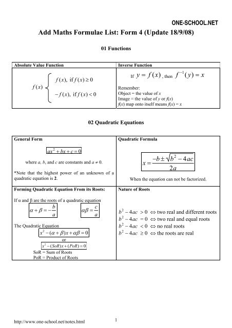
01 Functions
Absolute Value Function Inverse Function
f ( x)
General Form
ax 2 + bx + c = 0
where a, b, and c are constants and a ≠ 0.
*Note that the highest power of an unknown of a
quadratic equation is 2.
Forming Quadratic Equation From its Roots:
If α and β are the roots of a quadratic equation
b
α + β =−
a
f( x), if f( x) ≥ 0
− f( x), if f( x)
<
0
αβ =
The Quadratic Equation
2
x − ( α + β) x+
αβ = 0
or
2
x − ( SoR) x + ( PoR)
= 0
SoR = Sum of Roots
PoR = Product of Roots
1
If
02 Quadratic Equations
c
a
y = f( x)
, then
Remember:
Object = the value of x
Image = the value of y or f(x)
f(x) map onto itself means f(x) = x
Quadratic Formula
−1
f ( y) = x
x = −b ± b2 − 4ac
2a
When the equation can not be factorized.
Nature of Roots
b 2 − 4ac > 0 ⇔ two real and different roots
b 2 − 4ac = 0 ⇔ two real and equal roots
b 2 − 4ac < 0 ⇔ no real roots
b 2 − 4ac ≥ 0 ⇔ the roots are real

General Form
f ( x) = ax + bx+ c
where a, b, and c are constants and a ≠ 0.
*Note that the highest power of an unknown of a
quadratic function is 2.
a > 0 ⇒ minimum ⇒ ∪ (smiling face)
a < 0 ⇒ maximum ⇒ ∩ (sad face)
Quadratic Inequalities
a > 0 and f( x ) > 0 a > 0 and f( x ) < 0
a b
a
b
x < a or x> b
a< x< b
http://www.one-school.net/notes.html
2
03 Quadratic Functions
2
Completing the square:
f ( x) = a( x+ p) + q
ONE-SCHOOL.NET
(i) the value of x, x =− p
(ii) min./max. value = q
(iii) min./max. point = ( − p, q)
(iv) equation of axis of symmetry, x = − p
Alternative method:
f ( x) = ax + bx+ c
(i)
b
the value of x, x =−
2a
(ii)
b
min./max. value = f ( − )
2a
(iii) equation of axis of symmetry,
Nature of Roots
2
2
x =−
b
2a
2
b − 4 ac>
0 ⇔ intersects two different points
− =
at x-axis
⇔ touch one point at x-axis
2
b 4 ac 0
04 Simultaneous Equations
To find the intersection point ⇒ solves simultaneous equation.
Remember: substitute linear equation into non- linear equation.
2
b − 4 ac<
0 ⇔ does not meet x-axis

Fundamental if Indices
Zero Index,
Negative Index,
Fractional Index
Fundamental of Logarithm
x
loga
y= x⇔ a = y
loga a = 1
x loga a = x
loga 1= 0
0 a = 1
1 a− =
1
a
a − 1 b
( ) =
b a
1
n n
a
a =
m
n n m
a
a =
http://www.one-school.net/notes.html
05 Indices and Logarithm
3
Laws of Indices
a
a
× a = a
m n m+ n
÷ a = a
m n m−n ( a ) a ×
=
m n m n
( ab) = a b
n n n
a n a
( ) =
b b
Law of Logarithm
n
n
log mn = log m + log n
a a a
m
loga = logam− logan
n
log a m n = n log a m
Changing the Base
log
log
a
a
b =
log
log c b
a
c
1
b =
log a
b
ONE-SCHOOL.NET

Distance and Gradient
When 2 lines are parallel,
Midpoint
Midpoint,
Parallel Lines
M
m = m .
http://www.one-school.net/notes.html
1
2
⎛ x + x y + y ⎞
,
⎝ 2 2 ⎠
1 2 1 2
= ⎜ ⎟
06 Coordinate Geometry
4
ONE-SCHOOL.NET
Distance Between Point A and C =
( ) ( ) 2
2
x − x + x − x
1
2
y2 − y1
Gradient of line AC, m =
x2 − x1
Or
⎛ y − int ercept ⎞
Gradient of a line, m =−⎜ ⎟
⎝ x − int ercept ⎠
Perpendicular Lines
When 2 lines are perpendicular to each other,
1
m1× m2
=− 1
m1 = gradient of line 1
m2 = gradient of line 2
A point dividing a segment of a line
A point dividing a segment of a line
⎛nx1+ mx2 ny1+ my2
⎞
P = ⎜ , ⎟
⎝ m+ n m+ n ⎠
2

Area of triangle:
Area of Triangle
1
=
2
1
A = xy + xy + xy − xy+ xy + xy
2
( 1 2 2 3 3 1) ( 2 1 3 2 1 3)
Equation of Straight Line
Gradient (m) and 1 point (x1, y1)
given
y− y = m( x− x )
1 1
http://www.one-school.net/notes.html
2 points, (x1, y1) and (x2, y2) given
y − y y − y
=
x − x x − x
1 2 1
1 2 1
Equation of perpendicular bisector ⇒ gets midpoint and gradient of perpendicular line.
5
ONE-SCHOOL.NET
Form of Equation of Straight Line
General form Gradient form Intercept form
ax + by + c = 0
Information in a rhombus:
A B
D
C
y = mx+ c
m = gradient
c = y-intercept
x y
+ = 1
a b
a = x-intercept
b = y-intercept
x-intercept and y-intercept given
x y
+ = 1
a b
b
m = −
a
(i) same length ⇒ AB = BC = CD = AD
(ii) parallel lines ⇒ mAB = mCD
or mAD = mBC
(iii) diagonals (perpendicular) ⇒ mAC × mBD
=− 1
(iv) share same midpoint ⇒ midpoint AC = midpoint
BD
(v) any point ⇒ solve the simultaneous equations

Measure of Central Tendency
Mean
Median
Ungrouped Data
Σx
x =
N
x = mean
Σ x = sum of x
x = value of the data
N = total number of the
data
m= T N + 1
2
When N is an odd number.
TN + TN
+ 1
2 2 m =
2
When N is an even
number.
Measure of Dispersion
variance
Standard
Deviation
Ungrouped Data
2
2 ∑ x
σ = − x
N
σ =
variance
( ) 2
x x
σ =
Σ −
N
σ =
2
Σx
− x
N
http://www.one-school.net/notes.html
2
2
07 Statistics
7
ONE-SCHOOL.NET
Grouped Data
Without Class Interval With Class Interval
x
Σ fx
=
Σ f
x = mean
Σ x = sum of x
f = frequency
x = value of the data
m= T N + 1
2
When N is an odd number.
TN + TN
+ 1
2 2 m =
2
When N is an even number.
x
Σ fx
=
Σ f
x = mean
f = frequency
x = class mark
(lower limit+upper limit)
=
2
1 ⎛ N F ⎞
2 −
m = L+
⎜ C
f ⎟
⎝ m ⎠
m = median
L = Lower boundary of median class
N = Number of data
F = Total frequency before median class
fm = Total frequency in median class
c = Size class
= (Upper boundary – lower boundary)
Grouped Data
Without Class Interval With Class Interval
∑
2 fx
σ = − x
∑ f
σ =
2
variance
( ) 2
x x
σ =
Σ −
N
σ =
2
Σx
− x
N
2
2
∑
2 fx
σ = − x
∑ f
σ =
σ =
2
variance
( ) 2
Σ f x−x Σ f
2
Σ fx
σ = −x
Σ
f
2
2

The variance is a measure of the mean for the square of the deviations from the mean.
The standard deviation refers to the square root for the variance.
Effects of data changes on Measures of Central Tendency and Measures of dispersion
Measures of
Central Tendency
Measures of
dispersion
Terminology
Convert degree to radian:
Convert radian to degree:
Remember:
�
180 = π rad
�
360 = 2π rad
180
�
×
π
radians degrees
π
× �
180
http://www.one-school.net/notes.html
08 Circular Measures
8
ONE-SCHOOL.NET
Data are changed uniformly with
+ k − k × k ÷ k
Mean, median, mode + k − k × k ÷ k
Range , Interquartile Range No changes × k ÷ k
Standard Deviation No changes × k ÷ k
Variance No changes × k 2
???
0.7 rad
o π
x = ( x×
)radians
180
180
xradians = ( x×
)degrees
π
O
???
1.2 rad
÷ k 2

Length and Area
Arc Length:
s = rθ
Length of chord:
θ
l = 2rsin 2
Gradient of a tangent of a line (curve or
straight)
Differentiation of Algebraic Function
Differentiation of a Constant
y = a a is a constant
dy
= 0
dx
Example
y = 2
dy
= 0
dx
dy δ y
=
lim ( )
dx δ x→0
δ x
http://www.one-school.net/notes.html
Area of Sector:
1
2
2
A = r θ
09 Differentiation
9
Area of Triangle:
1
2
2
A = r sinθ
Differentiation of a Function I
n
y = x
dy
= nx
dx
n−1
Example
3
y = x
dy 2
= 3x
dx
Differentiation of a Function II
y = ax
dy
=
dx
= =
Example
y = 3x
dy
= 3
dx
11 − 0
ax ax a
ONE-SCHOOL.NET
r = radius
A = area
s = arc length
θ = angle
l = length of chord
Area of Segment:
1
2
2
A = r ( θ −sin
θ )

Differentiation of a Function III
n
y = ax
dy
= anx
dx
n−1
Example
3
y = 2x
dy
= 2(3) x =
6x
dx
2 2
Differentiation of a Fractional Function
1
y = n
x
Rewrite
−n
y = x
dy −n−1 −n
=− nx =
dx x
Example
1
y =
x
−1
y = x
dy −2
−1
=− 1x
= 2
dx x
Law of Differentiation
n+
1
Sum and Difference Rule
y = u± v u and v are functions in x
dy du dv
= ±
dx dx dx
Example
3 2
y = 2x + 5x
dy
2 2
= 2(3) x + 5(2) x= 6x + 10x
dx
http://www.one-school.net/notes.html
10
Chain Rule
ONE-SCHOOL.NET
n
y = u u and v are functions in x
dy dy du
= ×
dx du dx
Example
2 5
y = (2x + 3)
2
du
u = 2x + 3, therefore = 4x
dx
5 dy 4
y = u , therefore = 5u
du
dy dy du
= ×
dx du dx
= ×
= 5(2x + 3) × 4x= 20 x(2x + 3)
4
5u 4x
2 4 2 4
Or differentiate directly
n
y = ( ax+ b)
dy
n−1
= na ..( ax+ b)
dx
2 5
y = (2x + 3)
dy
= 5(2x dx
+ 3) × 4x= 20 x(2x + 3)
2 4 2 4

Product Rule
y = uv u and v are functions in x
dy du dv
= v + u
dx dx dx
Example
3 2
y = (2x+ 3)(3x −2 x −x)
3 2
u = 2x+ 3 v= 3x −2x −x
du dv 2
= 2 = 9x −4x−1 dx dx
dy du dv
= v + u
dx dx dx
3 2 2
=(3x −2 x − x)(2) + (2x+ 3)(9x −4x−1) Or differentiate directly
3 2
y = (2x+ 3)(3x −2 x −x)
dy 3 2 2
= (3x −2 x − x)(2) + (2x+ 3)(9x −4x−1) dx
http://www.one-school.net/notes.html
11
Quotient Rule
ONE-SCHOOL.NET
u
y = u and v are functions in x
v
du dv
v − u
dy
= dx dx
2
dx v
Example
2
x
y =
2x+ 1
2
u = x v= 2x+ 1
du dv
= 2 x
= 2
dx dx
du dv
v − u
dy
= dx dx
2
dx v
2
dy (2x + 1)(2 x) −x(2)
=
2
dx (2x + 1)
2 2 2
4x+ 2x− 2x 2x + 2x
=
= 2 2
(2x+ 1) (2x+ 1)
Or differentiate directly
2
x
y =
2x+ 1
2
dy (2x + 1)(2 x) −x(2)
=
2
dx (2x + 1)
2 2 2
4x+ 2x− 2x 2x + 2x
=
= 2 2
(2x+ 1) (2x+ 1)

Gradients of tangents, Equation of tangent and Normal
If A(x1, y1) is a point on a line y = f(x), the gradient
of the line (for a straight line) or the gradient of the
tangent of the line (for a curve) is the value of dy
dx
when x = x1.
Maximum and Minimum Point
At maximum point,
dy
0
dx =
2
d y
2
0
dx <
http://www.one-school.net/notes.html
dy
Turning point ⇒ 0
dx =
12
Gradient of tangent at A(x1, y1):
dy
dx =
ONE-SCHOOL.NET
gradient of tangent
Equation of tangent: y− y1 = m( x− x1)
Gradient of normal at A(x1, y1):
m
normal
1
=−
m
tangent
1
= gradient of normal
−
dy
dx
Equation of normal : y − y1 = m( x− x1)
At minimum point ,
dy
0
dx =
2
d y
2
0
dx >

Rates of Change Small Changes and Approximation
dA dA dr
Chain rule = ×
dt dr dt
If x changes at the rate of 5 cms -1 dx
⇒ 5
dt =
Small Change:
δ y dy dy
≈ ⇒δy≈ × δ x
δ x dx dx
Approximation:
Decreases/leaks/reduces ⇒ NEGATIVES values!!!
ynew = yoriginal + δ y
dy
= yoriginal + × δ x
dx
http://www.one-school.net/notes.html
13
ONE-SCHOOL.NET
δ x = small changes in x
δ y = small changes in y
If x becomes smaller ⇒ δ x =
NEGATIVE

Sine Rule:
a
sin A
=
b
sin B
c
sin C
Use, when given
� 2 sides and 1 non included
angle
� 2 angles and 1 side
a
b
A
http://www.one-school.net/notes.html
=
a
B
A
180 – (A+B)
10 Solution of Triangle
Cosine Rule:
a 2 = b 2 + c 2 – 2bc cosA
b 2 = a 2 + c 2 – 2ac cosB
c 2 = a 2 + b 2 – 2ab cosC
b
cos A =
2
14
2
+ c − a
2bc
Use, when given
� 2 sides and 1 included angle
� 3 sides
a
b
A
a
b
2
c
Area of triangle:
C
ONE-SCHOOL.NET
a
b
1
A = absin C
2
C is the included angle of sides a
and b.

Case of AMBIGUITY
C B′
B
Case 1: When a< bsin A
CB is too short to reach the side opposite to C.
Outcome:
No solution
Case 3: When a > bsin A but a < b.
CB cuts the side opposite to C at 2 points
Outcome:
2 solution
Useful information:
b
a
c
θ
180 - θ
A
http://www.one-school.net/notes.html
θ
15
ONE-SCHOOL.NET
If ∠C, the length AC and length AB remain unchanged,
the point B can also be at point B′ where ∠ABC = acute
and ∠A B′ C = obtuse.
If ∠ABC = θ, thus ∠AB′C = 180 – θ .
Remember : sinθ = sin (180° – θ)
Case 2: When a = bsin A
CB just touch the side opposite to C
Outcome:
1 solution
Case 4: When a > bsin A and a > b.
CB cuts the side opposite to C at 1 points
Outcome:
1 solution
In a right angled triangle, you may use the following to solve the
problems.
2 2
(i) Phythagoras Theorem: c= a + b
(ii)
Trigonometry ratio:
sin θ = , cos θ = , tanθ
=
b a b
c c a
(iii) Area = ½ (base)(height)

http://www.one-school.net/notes.html
11 Index Number
Price Index Composite index
I
P
1 = ×
P0
100
I = Price index / Index number
P0 = Price at the base time
P1 = Price at a specific time
I I I
AB , × BC , = AC , ×
100
16
ΣWi
I
I =
ΣW
I = Composite Index
W = Weightage
I = Price index
ONE-SCHOOL.NET
i
i