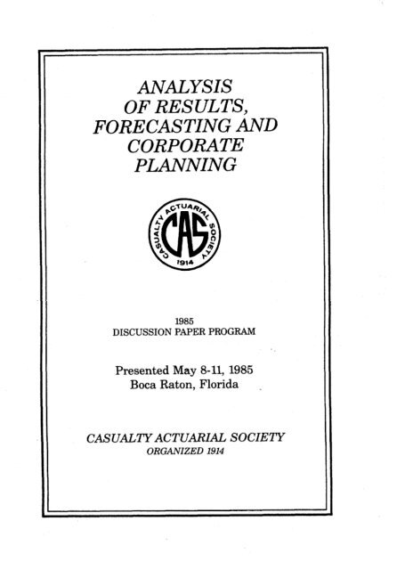
1985 DISCUSSION PAPER PROGRAM - Casualty Actuarial Society

ANALYSIS
OFRESULTS,
FORECASTINGAND
CORPORATE
PLANNING
1985
DISCUSSION PAPER PROGRAM
Presented May 8-11, 1985
Boca Raton, Florida .
CASUALTYACTUARIAL SOCIETY
ORGAhVZED 1914

ANALYSIS OF RESULTS,
FORECASTING AND CORPORATE PLANNING
These papers have been prepared in response to a call for papers by the Casualty Actuarial Society
to provide discussion material for its Spring meeting, May 8-11, 1985, in Boca Raton, Florida.
Actuaries have been becoming increasingly involved in all aspects of corporate planning and are
often called upon to explain results to people without technical or insurance backgrounds. It is hoped
that these papers will serve as the basis for a stimulating discussion at the Spring meeting while estab-
lishing a foundation for further research in these areas.
NOTICE
Committee on Continuing Education
The Casualty Actuarial Society is not responsible for statements or opinions expressed in the papers
in this publication. These papers have not been reviewed by theCAS Committee on Review of Papers.

Title
TABLE OF CONTENTS
Corporate Planning-An Approach for an Emerging
Company IreneK.Bass&LarryD.Carr
Crum and Forster Personal Insurance
Branch Office Profit Measurement for Property -
Liability Insurers Robert P. Butsic
Fireman’s Fund Insurance
Companics
A Formal Approach to Catastrophe Risk Assessment
and Management Karen M. Clark
Commercial Union Insurance
Companies
Measuring the Impact of Unreported Premiums
on a Reinsurers’ Financial Results DouglasJ. Collins
Tillinghast, Nelson &
Warren, Inc.
Bank Accounts as aToo for Retrospective
Analysisof Experience on Long-Tail
Coverages Claudia S. Forde and
W. James MacCinnitie
Tillinghast, Nelson &Warren, Inc.
Page
5-24
2.5-61
62- 103
104- 125
126-139

Title
I Projections of Surplus for Underwriting
Strategy William R. Gillam
North American Reinsurance
Interaction ofTotal Return Pricing and Asset
Management in a Property/Casualty
Company . . . Owen M. Gleeson
General Reinsurance Corporation
An Econometric Model of Private Passenger
Liability Underwriting Results RichardM. Jaeger and
Christopher J Wachter
Insurance Services Office, Inc.
Contingency Margins in Rate Calculations Steven G. Lchmann
State Farm Mutual Automobile
Insurance Company
Budget Variances in Insurance Company
Operations George M. Levine
National Council on
Compensation Insurance
Page
140- 171
l72- 194
195-219
220-242
243-267
B Pricing, Planning and Monitoring of Results:
An Integrated View . Stephen P. Lowe 268-286
Tillinghast, Nelson&Warren, Inc.

Title
The Cash Flow of a Retrospective
Rating Plan Glenn Meyers
The University of Iowa
Page
287-310
Application of Principles, Philosophies and
Procedures of Corporate Planning to
Insurance Companies Mary Lou O’Neil 311-331
New .Jersey Department of Insurance
Measuring Division Operating
Profitability DavidSkumick
Argonaut Insurance Company
q Actuarial Aspects of Financial
Reporting Lee M. Smith
Ernst & Whinney
332-342
343-372
4 Projecting Calendar Period IBNR and
Known Loss Using Reserve Study Results Edward W. Weissner and 373-424
ArthurJ. Beaudoin
Prudential Reinsurance Company

TITLE: CORPORATE PLANNING -- AN APPROACH FOR AN EMERGING COMPANY
AUTHORS: Irene K. Bass is Vice President of the U.S. Fire
Insurance Company and Actuarial Department head for
Crum and Forster Personal Insurance. Prior to joining
Crum and Forster, Miss Bass held positions at Commercial
Union and Hanseco. She is a Fellow of the Casualty
Actuarial Society and a Member of the American Academy of
Actuaries. She holds a B.A. in German from Bowling Green
State University and an M.S. in mathematics from
Northeastern University.
Larry D. Car-r is Senior Vice President and Chief Financial
Officer of the U.S. Fire Insurance Company with
responsibility for the Underwritina. Actuarial, and
Financial and- Planning areas of Crum aid Forster Personal
Insurance . He serves as a member of the Board of
Directors and Executive Committee of the U. S. Fire
Insurance Company. Mr. Carr had extensive experience, at
Allstate Insurance Company prior to joining CFPI in 1983.
He holds a B.S. in finance from the University of
Illinois.
ABSTRACT: A major property-casualty insurance group recently
created a separate profit center for personal lines,
thereby signaling a new emphasis on these lines. Since
the group had been a carrier with primary emphasis on
commercial business, the planning process at the personal
lines profit center became similar to that of an emerging
company: there was little relevant history available to
use in order to plan effectively for a very different
future.
Because planning at insurance companies is too often
separated from field operations -- the very people who
must make the plan happen -- we installed a process that
is operationally driven.
We therefore developed an approach to premium and loss
planning which did not rely on a simple projection of last
year's results. The major benefit of this planning
process is its lack of dependence on historical
information and its explanation of current results in
terms of specific components of the plan. We offer to
share and discuss this approach to personal lines
planning.
-j-

INTRODUCTION
Not too long ago, our insurance group reorganized and created, along
with several commercial lines profit centers, a separate profit
center for personal lines. Traditionally, the group's personal lines
volume was a relatively minor part of its total business,
representing about one-fourth of total premium. As such, there was
no special attention paid to it in the corporate planning process.
The profit center's new management, with its singular responsibility
for personal lines, initiated a planning process with five basic
goals in mind:
1. To build an operationally driven planning system from which the
financial plan would follow
2. To isolate measurements which are controlled -- or at least
influenced -- by line management
3. To insure commitment to the planning process by involving field
management in selecting planned levels of performance
To create a plan optimal for personal lines which would work in
an environment where the historical results would not necessarily
be an accurate predictor of the future
To blend the annual operating and financial plans into the profit
center's strategic plan.
-6

Although the personal lines volume is substantial, this new profit
center is an emerging company in the sense that the past will
probably not be representative of the future. It is also an emerging
company in terms of appointment of agents separately from the
remainder of the corporation, planned growth within the American
agency system, and independently defined goals, objectives, and
marketing strategies.
This paper is intended to illustrate a premium and loss planning
process for a personal lines company in a changing or emerging
environment. Expense planning is an important phase of all planning,
but the scope of this paper will be limited to premiums and losses
only. Our planning process is fairly straightforward in terms of the
mathematical concepts employed. It is not simply a matter of
determining last year's results and then making some estimates for
the coming year. Rather, each component of the premium is analyzed
down to the basic elements, beginning with number of agents and
ending with premium. Likewise, losses are analyzed in their
elementary components of frequency and severity.
In this paper we first offer some background on the difficulties of
planning for an emerging company and obtaining the proper source data
to do a zero-base analysis. Then we discuss the premium and loss
planning methods. Finally, we evaluate what was accomplished in the
planning process.
-7-

BACKGROUND
The operational plan is segmented into three separate but connected
pieces:
- Agent Plan
- Production/Premium Plan
- Losses Plan
These represent the major planning decision areas in which baseline
values and the impact of operational changes must be established.
Charts of the detailed statistical flow are contained in Exhibits
3-5. Once a conceptual understanding of this flow is achieved, four
things are required to plan:
1. Base Data -- the explicit values of the variables in the
equations to get from number of agents to premiums to incurred
losses.
2. Operational Plans -- the expected changes in operating
philosophy, approach, and execution. This information is based
on the continuing analysis of programs and their results and on
management's evaluation of areas where current performance
requires improvement.
3. Quantification of Plans -- the specific numerical ramifications
of operational plans. If operational plans are carefully
-8-

prepared within a structured framework and are based on objective
evaluation of data, this quantification is often completed in the
operational analysis process. If not, basic analysis to quantify
operational changes is required. This is a critical step in that
it allows management to see whether planned activity will achieve
desired results. This is the fundamental reason for planning.
4. External or Extraordinary Factors -- the impact of any
anticipated changes in external factors. These factors must also
be isolated and considered. Extraordinary weather-related claim
volume in the historical data is an example of this kind of
influence.
The planning model -- composed of the variables in the planning
equations and the equations themselves -- is fundamentally important
in that it allows for measuring the impact of planned actions on
operating results.
Because this profit center is a personal lines operation emerging
from a predominantly commercial lines environment, it is not
surprising that the kind of data we sought was not available from
readily accessible sources. Therefore, the acquisition of base data
was the most difficult part of the process and certainly the most
time-consuming. Annual Statement and Insurance Expense Exhibit data
do not provide sufficient detail for an operationally driven plan.
New and renewal production, frequency, and severity data just do not
exist in these sources. At our company, it also required compromises
regarding the desired breakdown of data by line of business.
-9-

It became obvious that ideal information was not to be found, so we
settled on the following compromise prioritization.
1. Necessary data would become available over time, so the most
important aspect was the integrity of the statistical flow. When
a source of net written premium by desired line of business did
not have a companion policy count report, we chose a summary
level that preserved the desired statistical flow. More
important than planning by ideal product line, it was essential
to begin installing the operational discipline, involving field
management in the planning process, and planning in a fundamental
step-by-step method that would permit isolating the sources of
variance from plan.
2. Because of the need to focus on markets, results, constraints,
and opportunities on a state-by-state basis, higher levels of
product summarization were accepted than was desired. For
example, homeowners was handled as one line rather than
separating it into owner, renter, and condo business.
3. When all else failed and source data was not to be found, prior
experience, judgment, and estimates were often used.
We often used sources for purposes other than their original intent.
Agent counts were developed from a monthly report used to check
validity of mailing lists. New business production and renewal
ratios were derived by an elaborate manipulation of in-force policy
counts and cancellation activity. New business and renewal premiums
-lO-

were generated from reports originally prepared to measure processing
through the underwriting department. Claim counts -- and,
ultimately, frequency and severity -- were completed using claim
department workload reports.
STATISTICAL MODEL
The premium planning process is outlined on Exhibits 1-4. Loss
planning is outlined on Exhibit 5.
Agents
The process begins with the agent plan and develops into premium on a
line of business basis.
Because of the radically changing environment in the company, we
could not begin with last year's premiums and project forward. We
knew we would be cancelling personal lines contracts for many agents
who were commercial lines oriented and appointing new agents for
personal lines only. Since this activity is part of regional
management's objectives, it made sense to involve them in the
quantification of the number of active agents and to have this item
become a measurable variable in the plan. This is an example of
field management involvement and of the isolation of measurements
that are controlled or influenced by them.
-ll-

Production
Average number of new policies per agent was calculated by line of
business from prior years, and an estimate for the ensuing year was
based on several assumptions. This number would be very different
from prior years because now we would be dealing with agents who are
primarily personal lines agents and who would use our company as a
major market, Agency management would be directed at personal lines
only, and major changes in pricing would shift our competitive
position.
By multiplying average number of agents by number of new policies we
obtained the total number of new policies issued for each line
(Exhibit 1). But renewals also had to be calculated. The prior
year's policies (which become available for renewal this year) were
multiplied by a renewal ratio to obtain the number of renewal
policies issued (Exhibit 2). Careful analysis of the renewal ratio
was necessary since the expected termination of some agents and the
planned re-underwriting programs would most likely cause this ratio
to drop. At the same time, improved policy service and changes in
the mix of business would tend to increase the renewal ratio.
Premium
The next step starts with number of policies issued and ends with
the net written premium (Exhibit 3). New policies must be handled
separately from renewal policies when estimating the average written
premium by line of business. New business, given the thrust to
-12-

appoint primarily personal lines agents and to penetrate a different
market sector, should have a significantly different average premium
from prior period business that will be renewing. For example, an
effort to write many more homes of high value will cause the average
premium to be much higher.
Even the average renewal premium might be very different from prior
years. If, as in the prior example, an effort to penetrate the high-
value homeowners market is coupled with competitive pricing in that
segment, changes in homeowners relativity curves may greatly increase
the premiums charged for low-valued dwellings. Re-underwriting and a
campaign to insure to value may also increase these averages. In our
plan, field management input along with information from the pricing
actuaries was needed to quantify this variable.
Gross written premium is obtained by multiplying the number of
policies issued by the average premium separately for new and renewal
policies (Exhibit 3). Endorsement premium is loaded by means of a
factor and the remainder of the steps leading to net written premium
are straightforward.
Earned premium and policies in force are important by-products of the
statistical flow (Exhibit 4). Neither is planned directly: they flow
from the numbers being generated by the internal relationships of the
model. By developing a historical relationship between formula
earned premium (l/24 of current month's written premium plus l/12 of
prior eleven months' written, plus l/24 of twelfth prior month's
written) and actual monthly earned premium, a clear pattern should
-13-

develop which will establish an appropriate relationship between
formula and actual earned premium (Exhibit 4).
At this point in the flow, developing the earned premium involves
only selecting an appropriate earned premium compensating factor and
doing the arithmetic. Policies in force (new and renewal separately)
are arrived at by accumulating all of the policies that could be in
force from the prior 12 months' policies issued and applying an
appropriate termination rate.
Losses
Once the premium plan is complete, the generation of incurred losses
essentially flows out of a continuation of the logic. Policies in
force become the base against which frequency ratios (new business
separately from renewals) are applied to arrive at claim counts
(Exhibit 5). It is important that the assumptions about changes in
the agency force, market focus, and underwriting rules be carried
through to frequency selection. Otherwise, loss ratios will be
distorted.
Claim counts can then be multiplied by an appropriate severity to
arrive at losses (Exhibit 5). A number of different approaches are
possible here but, essentially, historical levels are modified to
reflect expected changes in average claim costs due to inflation,
changes in mix of business, limits, deductible, etc. The
effectiveness of the claims department must also be reflected. IBNR
reserve changes can then be added to incurred losses before arriving
at the final loss ratio.
-14-

It is important to recognize that the various operational action
plans are quantified in very different ways in the development of the
plan. A careful evaluation of the loss ratio will help insure that
the impact of various operational plans is consistently assessed in
determining both premium-related and loss-related base data,
EVALUATIOH
A number of legitimate questions seem obvious. With all the
compromises in data, did the process really accomplish anything? Was
the cost in time and effort appropriate in the completely manual
environment? In short, was it worth the effort? Our answer is an
unequivocal, "Yes," because several very important baselines were
established, as discussed below.
1. A base of information was developed.
2. Management became more in touch with the company's expected
results more quickly than it would have without the planning
process.
3. An operationally based planning process was installed. Accepting
that the first plan would be the worst, we decided it was
important to install the process in order to begin its evolution.
We could not have waited another year to begin establishing those
disciplines and thought processes.
-15-

4. The planning process clearly established the relationship between
functional management and results. Operational actions -- the
changes, refinements, and corrections -- are necessary if results
are to change.
5. A set of performance benchmarks were established. They could
have been established in a number of other less time-consuming
ways. But the advantage of this approach is that when actual net
written premiums or incurred losses are different from plan, the
source of the difference can be specifically identified and
evaluated. From an informed perspective, management can then
decide to accept the variance or take action to correct it.
CONCEPTUAL MODEL
Critical questions to ask in an operationally based planning process
include:
Market Direction -- Will there be any changes in products, geographic
focus, or target market segments? Will there be changes in the
relationship with agents such as new profit-sharing agreements,
increased or decreased leverage, or an agency force restructuring?
All of these areas could impact assumptions about agents,
productivity, renewal trends, average premium, retention, losses, and
expenses.
-16-

Pricing Philosophy -- Are there going to be changes in price,
competitiveness, or rating schemes to attract certain risks? These
will also impact nearly all parts of the statistical flow.
Underwriting Approach -- Will any changes occur in underwriting rules
which could impact production and average premiums as well as losses?
Changes in emphasis on policy limits, deductibles, or sale of
optional coverages should also be carried thrbugh to the numbers
selected. It. is important to evaluate the impact of past
underwriting decisions that could be "cycling through" their period
of impact, e.g., a re-underwriting program begun in the middle of the
prior year.
Level of Service -- Strong correlations exist between retention and
.
the level of policyholder/claim service. What will be the impact of
anticipated changes in level of service whi&h should be considered in
developing renewal and retention levels and changes?
Claims Handling Practices -- How will opening and closing practices,
different emphasis on case reserve adequacy, clearing backlogs, etc.,
influence both frequency and severity measurements?
Once a consensus on these five areas is achieved, only one conceptual
step remains: environmental issues need to be examined. Inflation,
unemployment, housing starts and car sales, trends in miles driven,
gasoline prices, and so on, all impact key planning variables. So,
too, do the actions of competitors, regulators, and legislators as
-17-

their collective modifications of the environment influence the
effectiveness of our actions.
At this point, the truly difficult part of planning is finished. The
remaining work involves, simply, a translation of these operational
and environmental conclusions into statistical impact. It is at this
point that the planner needs extraordinary discipline. There will be
times when, after all the work is completed, the results are
unsatisfactory -- management can't live with the bottom line.
An easy way to correct this situation is simply to change a number.
If this happens, the entire planning process is invalidated and
displeasure with planned performance quickly becomes dismay over
actual results. When unacceptable results are projected in the
planning process, only two valid actions can be taken. First, the
translation of concepts to numbers should be rechecked. Any mistakes
should be corrected and the numbers recalculated. If this does not
correct the problem of unacceptable results, management must return
to its basic assumptions about operations and modify them to achieve
acceptable results.
Only in this way is it possible to arrive at financial plans based on
sound operating decisions. Only with this detailed approach can the
future sources of variance be isolated and corrected.
-18-

Discussion Questions
1. If results are different from plan, does this method allow one to
identify the cause of the variation? Does it pinpoint the cause
sufficiently for management to take proper corrective action?
2. Is this approach adaptable to planning in the commercial lines
environment?
3. Is an operationally focused, detailed plan really needed in the
insurance industry?
4. What sort of controls are necessary to insure the integrity of
the plan?
5. Will this approach be effective for an emerging company or does
it require an established company "culture"?
-19-

NEW PRODUCTION
-_--m-e--- --
I I
; Average # Of Agents i
L---- ------ -J
X
I Average Policies Per Agent ,
I I
---------------’
Prepared by line of business
-2o-
Exhibit 1

RENEWAL PRODUCTION
---------------------t
7
Prior Year I
1 New Policies Issued 1
I i
I ---------------------- J
------------------------.
I
Prior Year
t , Renewal Policies Issued
I .------------------------
Renewal Policies Issued
+
Prepared by line of business
-21-
1
t
Exhibit 2

X
_--------- e-m
I
I New I
1 Average Premium I
_-_--- -----
PREMIUM Exhibit 3
Endorsements
7--- ---- -- “7
[Cancellation Ratio:
t
------_-a
I
f Reinsurance Ratio I
I ----_ T------!
Prepared by line of business
-22-
I
X
-_---- --------
I
f Renewal I
Average Premium I
----- -7----

1 I
I *'Formula"
Earned I
EARNED PREMIUM
AND
POLICIES IN FORCE*
X X
--------w
r-
I
t Earned Premium
I I
! Compensating ,
I -----_-_
I
Prepared by line of business
12 Month Moving
Policies Issued I
r- --------I
iPolicies in Ibrce/i
,
c
Policies
Retention
m-m-
Issued
Ratio
---.4
1
I
*Policies in force calculated separately for new and renewal
-23-

LOSSES Exhibit 5
1 Policies In Force 1
r------------,
X
I Proportion
I
(auto
- ----of
Coverages
only)**
-__-__
I
I
I
+
Coverages in Force
X
---
FFrequency 7
I ------I
X
l- -----l
I Severity I
i-----J
I
IBNR
I
I
/Total Losses 1
Earned Premiu
&I
Loss Ratio
Prepared by Line of Business
**Prepared by Coverage for Auto
-24-

BRANCH OFFICE PROFIT &BASIJREMENT FOR PROPERTY-LIABILITY INSURERS
Robert P. Butsic
Biographical Sketch
Current employer is Fireman's Fund Insurance Co.; prior affiliation was with CNA
Insurance from 1969-1979. Earned BA in Mathematics in 1967 and MBA (Finance) in
1978, both from the University of Chicago. Associate in Society of Actuaries,
1975; Member of American Academy of Actuaries. Wrote papers for previous CAS
Call Paper programs in 1979 ("Risk and Return for Property-Casualty Insurers")
and 1981 ("The Effect of Inflation on Losses and Premiums for Property-Liability
Insurers").
Abstract
Effective measurement of financial performance for individual branch offices is
hindered by two major problems. The first is an appropriate definition of
profit; this is addressed through an economic-value accounting method which
minimizes distortions due to the timing of income recognition. Return on equity
is the basic profitability gauge used to compare results between profit
centers. The second problem is that, in comparing results between branches,
different levels of risk will produce an uneven chance of error in measuring true
performance vs. reported results. This problem is addressed through techniques
which equalize systematic risk (by implying an equity value) and non-systematic
risk (through internal reinsurance), for each branch. To develop the internal
reinsurance concept, a Poisson claim frequency and a Pareto claim severity model
is constructed. Finally, in order to recognize the credibility of each profit
center's actual experience, a canpromise is made to the equal-variance prin-
ciple. The analysis concludes that branch office profit measurement is best
served when the branch network has minimal variation in size and product mix.
-25-

BRANCH OFFICE PROFIT MEASUREMENT FOR PROPERTY-LIABILITY INSURERS
-26-

The insurance industry is presently becoming less regulated, creating an
increasingly competitive long-term environment. To effectively meet the
challenge posed by this new climate, insurers must strengthen their marketing and
get closer to the consumer. Consequently, a strong branch office network is
needed in order to cope with the variety and complexity of local conditions.
A major factor in the development of a viable branch office organization is the
principle that each branch is completely responsible for Its own contribution to
corporate profits. Hence, the profit center concept. Given the objective to
drive corporate profits from the sub-units which are held accountable, an
appropriate tool for measuring performance must be used.
The purpose of this paper, then, is to outline a general approach for measuring
the performance of individual profit centers comprising a property-casualty
company. The methods presented here could apply to line of business or regional
definitions of “profit center”, but it dll be most useful to think of a profit
center as a branch office.
The paper focuses on the aspects of profit measurement and presents methods
which equalize both systematic and purely random variation in profit center
results. Other Important aspects of profit measurement, including the accounting
treatment, are developed in lesser detail. Many of the thoughts presented here
have wolved wer time at the writer’s own company and are now being brought to a
practical application In its management reports.
-27-

Corporate Profitability
PROFIT I%- NT IW PEOPERlY-CA!XJALT’f INSRAIKE
Before addressing the profitability measurement of individual profit centers one
must first define an appropriate yardstick for the corporation as a whole. For
this important concept we will choose return on equity, or ROE for short. This
measure is commonly used for other industries, and represents the return to an
investor in the corporation (for further background on this topic, see references
141, 181 and [lol).
Although ROE is a simple concept, it must be carefully defined. The accounting
conventions used must be suitable for performance measurement over a reasonable
time frame such as a month, quarter or year. Stated differently, management
reports should encourage behavior which will tend to maximize the value of the
firm.
The return on equity measure can be separated into two components: net income
(the numerator> and equity (the denominator).
Net income must reflect, to the extent possible, the current impact of all future
transactions related to the premium earned in the current period. This means
that:
1. Accident-period accounting is used, with all losses, premiums,
expenses and dividends continually being restated as better
estimates of their ultimate values become known.
-2%

2. All future investment income earned on cash flows arising from
the current period must be recognized in the period. The usual
device for collapsing an income stream is net present value.
3. The future cash flows are taken to present value using a market
interest rate, and not the portfolfo rate. It should be noted
that the appropriate rate for corporate performance measurement
may differ from that for profit centers, due to the separation of
responsibility for investment and underwriting risk.
Equity, in a similar fashion, must be adjusted to reflect the above timing of
income:
1. All assets must be evaluated at market prices and all liabilities
must be discounted to present value (i.e., the market price in a
portfolio reinsurance transaction).
2. Otherwise, normal GAAP accounting for equity should be used.
The preceding concepts attempt to recognize what is bown in the accounting
literature (see Lev [SJ) a8 economic income -- the anticipated consequences of
current decisions are directly reflected in current earnings. The notion of
economic income can be further explained by a numerical example. Assume that a
miniature “company” is formed under the following circumstances:
1. An annual policy of $100 is written on January 1, 1985.
-29-

2. A single claim of $68.20 occurs on January 1, 1985 and is paid
over three years, as indicated in the following cash flow
schedule.
3. Cash transactions occur on January 1 of each year; the last loss
payment occurs in 1987.
4. Cash is invested at a yield of 10% per year.
5. All cash flows are certain.
6. There are no income taxes applicable.
7. Capital of $50 cash (initial equity) is available on December 31,
1984.
8. Expenses of $35 are paid on January 1, 1985.
The cash flows are shown below:
Cash Flow Schedule
l/l/85
Premium
Losses
Expenses
Total
- L/1/85
100
0
-35
65
- l/1/86
-44
-44
- l/1/87
-24.2
-24.2
Total
100
-68.2
-35
-3.2
Present Value
100
-60
-35
5
Here we see that the value of the policy to us at the time the premium was
written is $5.00. Under economic-value accounting, the balance sheet would look
like:
-3o-

Balance Sheet: Econanic Value
1984 1985 1986 1987
---- 12/31 l/l 12/31 111 - 12131 -iTi-
Assets 50.00 115.00 126.50 82.50 90.75 66.55
Loss Reserve 0 60.00 66*00 22.00 24.20 0
Eiquity 50.00 55.00 60.50 60.50 66.55 66.55
- Pres. Value (l/1/85) 50.00 55.00 55.00 55.00 55.00 55.00
The loss reserve here equals the present value of unpaid losses. Notice that
beginning l/1/85, the present value of equity is always $55.00, because no addi-
tional income is generated by the future cash flows arising from the insurance
operation (as opposed to re-investment of equity):
Underwriting Gain
Investment Income - Loss Reserves
Net Income - Insurance Operation
Investment Income - Equity
Net Income - Total
Income Statement: Economic Value
1985 1986 Total
-1 .oo -2.20 -3.20
6.00 2.20 8.20
5.00 0 5.00
5.50 6.05 11.55
10.50 6.05 16.55
This tabulation clearly shows that all income arising from the policy is recorded
-
in 1985, when the premium is earned. For comparison, the traditional accounting
method would give the following balance sheet end income statement:
-31-

Balance Sheet: Traditional Accounting
1984 1985
1986 1987
12/31 PI_ l/l 12/31 -- l/l 12131 -iT
Assets
50.00 115.00 126.50 82.50 90.75 66.55
Loss Reserve 0 68.20 68.20 24.20 24.20 0
Equity 50.00 46.80 58.30 58.30 66.55 66.55
- Pres. Value (l/1/85) 50.00 46.80 53.00 53.00 55.00 55.00
Income Statement: Traditional Accounting
- 1985 - 1986
Underwriting Gain
-3.20 0
Investment Income - Loss Reserves 6.82 2.42
Net Income - Insurance Operation 3.62 2.42
Investment Income - Equity 4.68 5.83
Net Income - Total 8.30 8.25
Total
-3.20
9.24
6.04
10.51
16.55
Notice that by the end of 1986 (a moment before the last cash transaction on
l/1/87) the accumulated equity is equivalent under either accounting method.
However, the timing of income recognition differs dramatically.
The preceding example illustrates some fundamental ideas which can be developed
more fully. The first is the concept of the total profit margin, or TPM. In
economic valuation, the issuance of the $100 policy created an instant “profit”
of $5; we are indifferent to selling the policy or accepting $5 in cash. This
total profit brought to present value is 5% of premium, hence a 5% total profit
margin.
The second is the economic return on equity. We started with $50 of equity and
one year later the economic value of the mini-enterprise is $60.50, yielding a
21% ROE.
-32-

More compactly, the ROE can bs represented by
(1) 1 + R = (1 + I)(1 + km),
where R denotes the (economic) return on equity, i the market (riskless) interest
rate, k the premium divided by initial equity, and m the total profit margin. To
verify the preceding example, we get 1 + R = l.l[l + 2C.0511 = 1.21.
Although traditional accounting may provide a reasonable means of aggregate
performance measurement for an insurer under conditions of stable growth,
interest rates and product mix, It can fail miserably at the individual profit
center level due to more severe timing distortions of income recognition (for
example, individual case reserve changes on prior period losses can be dramatic
for a single branch).
-33-

?RODUCT LINR PROFIT HMSIPPIIENT
Raving established the economic return on equity evaluation approach as a viable
aggregate profitability measurement, its application must be extended to
individual product lines.
Relative Risk
Although ROE is a good profit measure, there are problems associated with its use
in comparing insurance (and other types of) companies or product lines. These
difficulties arise because the amount of risk associated with an ROE measure
varies significantly by line of business. For example, given the option of
buying stock in a medical malpractice insurer with an expected ROE of 20% or in a
personal lines company of the same size having a 15% ROE, it is unclear what
choice to make. The medical malpractice insurer would be considered to have a
riskier return. The returns must be adjusted to equalize risk between various
types of coverage.
Here risk means systematic or process risk, which cannot be reduced (relative to
premium) by increasing the number of individual exposures. Examples of
systematic risk for property-liability insurance include:
1. uncertainty of ultimate losses due to length of time from
occurrence to final settlement,
2. uncertainty of ultimate loss due to future costs (inflation) being
higher than anticipated in pricing, and
-34-

3. uncertainty of loss costs arising fran lopfrequency events, such
as in municipal bond or nuclear reactor coverages.
Further discussion of systematic risk can be found in references 121, (41 and
[PI. Also, Appendix I provides a more rigorous treatment of this topic, showing
the difference between systematic and non-systematic (random) risk.
To adjust the ROE measure for risk, consider Equation (1) with the ROE and TPM as
random variables:
(2) 1+fi= (1 + I)(1 + kg,.
Here "m" denote8 a random variable. ‘l’he interest rate, being riSkleSS, is not a
randaa variable. Also, the premium/equity ratio k is a constant since it repre-
sents a known quantity. The variance and standard deviation of the ROE are given
by
(3a) Var(5 - (1 + 1)’ k* Va& and
(3b) a6 - (1 + I) kU(%.
In order to proceed further, the ROE risk will be defined es being equal to its
standard deviation. Thf8 is commonly used in financial theory (see Sharpe [ql,
for example) aid has the intuitively appealing and important property that it IS
independent of the scale of operation: two companies identical in all other
respects but size will have the same risk, measured in terms of variation fran
-35-

expected ROE. This definition is equivalent to that of systematic risk, which,
being independent of the number of exposures, is constant for e particular
product line, regardless of size.
For two different product lines (denoted by subscripts) one cBn equate the ROE
risk using (3b);
(ha) m+ - O(i2>-- klC(gl) = kg CC:,), or
(4b) O-Cm”, )/ ci(G,) = k2/kl.
’ In other words, two product lines have ident ical ROE risk when their
premium/equity ratios are inversely proportional to their respective measures of
systematic risk.
Risk Equalization
How do we measure systematic risk for property-liability lines of business?
Unfortunately, there is no objective way to measure some of the risk components,
such as the uncertainty of low-frequency events. Nevertheless, even a
judgemental approach is better than to assume that all lines have equal risk.
A suggested method for subjectively balancing risk for various product lines is:
-36-

1. Select a product line, say Commercial Multiple Peril, with an
average perceived risk. Assign to it an arbitrary premium/equity
ratio in the neighborhood of the long-term industry average
premium/equity ratio for all lines; e.g., 2.5-to-l.
2. Select another line, compare it to the standard line (CMP) and set
a premium/equity ratio at which you would be indifferent to writing
this line compared to the standard line. For example, Fire (having
a fast loss payout and a relatively complete pricing data base) at
a b-to-1 premium/equity ratio might be considered equally risky as
CMP at 2.5-to-l.
3. Repeat the process for all applicable product lines. Of course,
the method can be extended to sublines or even new types of
insurance.
This procedure, or one which actually attempts to measure the relative systematic
risk (see Pairley [l]), will produce imputed equity values for each line based
upon the respective premiums written. The aggregate all-lines imputed equity
need not equal the "actual" equity reported externally, since our intent is to
measure relative profitability between lines without having to be concerned about
their different absolute levels of risk.
Returning to the earlierquandary (medical melpractice et 20% ROE vs. personal
lines at 15% ROE), suppose that the medical malpractice ROE arises from a 5% TPM
having e standard deviation of 3X, while the personal lines TPM is 2% with a
standard deviation of 1%. The intereet rate is 10%.
-37-

Applying Equstion (2), the medical malpractice premium/equity ratio is 1.818 and
the personal lines ratio is 2.273. Equation (3b) gives a 6% medical malpractice
ROE standard deviation and a 2.5% value for personal lines. To equalize the ROE
risk, we increase the personal lines premium/equity ratio to 2.273(6/2.5) = 5.455
(conversely, we could decrease the malpractice premium/equity ratio by a factor
of 2.5/6), yielding an ROE standard deviation of 6%. However, the expected
personal lines ROE now increases to l.l[l + 5.455(.02)] - 1 = 22%. Therefore the
personal lines return would be superior to that of the medical malpractice
insurer.
The preceding calculations are summarized in the following table:
Before Equalization After Equalization
E(g) a(r;;> k E(ii) 6, k E(ii) a&
Medical Malpractice 5.0% 3.0% 1.82 20.0% 6.0% 1.82 20.0% 6.0%
Personal Lines 2.0 1.0 2.27 15.0 2.5 5.45 22.0 6.0
-38-

?ROFIT CSRTKRPSKEQIJIVALEXE
Raving developed the basis for equalizing systematic risk between product lines,
it ie nov possible to apply the method to a composite of various lines, namely
the profit center.
Systematic Risk Epuivalence Between Profit Centers
For the ccrmposite of two (or more) lines, there is an additional element vhich
tends to increase systematic risk - correlation betveen total profit margins.
Suppose that the implied equity for each line has been determined to equalize the
respective ROE risk. Let fl and f2 represent the respective proportions of the
total (fl + fq - 1) implied equity for each line, p the correlation coefficient
between il and z2, and the subscript t the results for the branch total. The
variance of the branch ROE is
(5) Var(Q = Var(Zl)[l - 2(1-fJ)flf21.
Appendix I derives this result. Notice that Var$) - Var( ii;) eince the ROE risk
has been equalized.
The following numerical example illustrates the preceding result:
Line(i) Premium
-II_ ki
Equity EG, 1 Gi, 1 E&i) 4,)
1 100 4.0 25 1.5% 1.0% 16.60% 4.4%
2 150 2.0 75 4.0% 2‘0% 18.80% 4.4%
Total 250 2.5 100 3.0% 1.6% 18.25% 4.4%
1.3% 3.5%
-39-
e
1
0

Notice that the standard deviation of the ROE for this branch will be reduced
(down to 3.5%) if the lines have total profit margins which are not fully
correlated.
Several observation8 can be made from the analysis so far:
1. To the extent that lines within a profit center are not perfectly correlated
in their TPM's, the overall ROE risk is reduced.
2. For a given correlation structure, the profit: center ROE risk reduction is a
function of the line mix.
3. Maximum risk reduction is attained when the line mix is such that the implied
equity amount 18 equal for each line (i.e., fl - f2 In Equation (5)).
For comparing results between two different profit centers, the theoretically
correct procedure would adjust the implied equity for each branch due to risk
reduction from line mix. However, this would be a formidable computational task
due to the large size of the relevant correlation matrix and the difficulty of
estimating the line correlation coefficients fran empirical data. A more
practical approach is to assume that the line mix among branches is such that
there will be a negligible variation in ROE risk due to intercorrelation.
Non-Systematic Risk: Poisson-Pareto Model
We have now reached the point where each profit center can be evaluated on the
basi8 of its own ROE given the equalization of systematic risk. Ideally, we
vould like to remove all sources of chance variation, systematic or otherwfse, in
-4o-

order to ascertain whether the masured result is the “true”, or inherent
result. However, as discussed earlier, systematic risk by it8 very nature 18
difficult to reduce since it is independent of the size of operation (loss ratio
reinsurance would work somewhat, but at the expense of a lower return). On the
other hand, non-systematic (or NS) risk can be trimmed more readily thrcugh
internal reinsurance. Increasing the number of exposure8 will also reduce NS
risk, but in practice the size of a profit center is severely constrained.
A major source of random risk for a profit center is large losses due to single
occurrences. Here we define a large loss as arising fran a single insured, to
distinguish natural (i.e., IS0 serial-number) catastrophes, which will be treated
later.
For a network of profit centers, the NS risk arieing fraa large claims can be
formulated readily using some simplifying assumptions:
1. A large loss is denoted by the random variable 2 9 r, where r is a reference
point above which we are willing to establish an internal excess 1088
refnsurance pool. Losses below r are assumed to be fixed in number and
amount, and do not contribute to the variance of total losses for the profit
center. For eimplicity of presentation we will henceforth sssume that these
losses are eero.
2. All individual losses arise fr(~~ a single product line and have the same size
distribution; however, the expected number Ni of large losses varies by
branch I.
-41-

3. The rumber of large losses gi has the Poisson distribution with parameter Ni.
4. The lose amount “x has the Pareto distribution, with parameter a (Patrik[‘l]
discusses the applicability of this assumption). Other functions, such as
the log-normal, are less computationally tractable, beside8 being unsuitable
for fitting the tail of loss size distributions. Basically, the 2 parameter
indicates the “tail thickness” of the loss size distribution: the higher the
value of a, the less likely a loss will occur at a higher level relative to a
lower level. Empirical evidence indicates that 2 varies between about 1.5
and 3, with low values for liability lines and high values for property
coverages. Appendix II gives more detail regarding the Pareto distribution.
5. All losses have the 8ame payment pattern. Thus, the present value of the
1013s g can be represented by dx”, where d is a constant.
6. The total premium for the profit center is collected when written and is
proportional to the expected losses. Since the average loss size is the same
for all branches, the premium, denoted by PNi, is proportional to the
expected number of large losses.
7. There are no expenses, only losses and premiums.
m total VahS of all loeses in a particular branch i is (subscript i removed
for clarity)
(6) g-f,+

where the number of losses G is also a randan variable with expectation N.
Because s is a compound Poisson distribution it has mean and variance (see
Appendix 111 for derivation):
(7a) E(Z) - NE& - Nra/(a-1) and
(7b) Var(3 - NE(ji2) + N2C - Nr2a/(a-2) + N2C,
where C - Cov(ji,,iij) 18 the covariance between two Separate losses zk and i$*
The total profit margin for the profit center is
(8) ii = (PN - d$)/PN.
The variance of the TPM is, from (7b) and (81,
(9) Var(m”) -$[ E(r) + “3.
Notice that as N becomes infinite, the variance of the branch TPM is proportional
to the covariance of individual losses; i.e., only systematic risk is present.
This result is consistent with the basis for selection of the implied
premium/equity ratios for different product lines. However , in the large loss
model here, we have assumed a single line and therefore the covariance C is the
8ame for all branches as is the premium/equity ratio. Consequently, equating the
ROE risk for two branches implies that E(“x2)/N must be the same for the branches.
Because the loss size distribution is the same for all profit centers, but the
expected number of lOS8eS N may vary (in fact, N defines the size of the branch),
the siee of loss dietrfbution must be transformed 80 that the second moment E(z2)
can vary by branch. The common mechanism for achieving this goal is excess
refnsurance.
-43-

To do this, we select a retention br > r , where b is a scaling factor. Now let
Y = g for r i x” ( br and 7 - br for z > br. In other words, the loss is
“stopped” at a value of br. For this protect ion, we charge the branch an amount
8uCh that its expected total losses remain equal to N?(g). As shown in
Appendix II, the expected portion of a Single loss retained in the interval r to
br is
(10) (l-b’-a)E(ii’> = (l-blma) ar/(a-1),
and the expected ceded amount above br 18
(11) blVaE(X”) - blsa ar/(a-1).
Also shown in Appendix II, under the Pareto distribution, the second moment of
the retained loss size becomes
(12a) E(T2) = r2(a - 2b2-a )/(a-2) for a $ 2,
(12b) E(F2) = r2[1 + 2 In(b)] for a = 2.
To determine the relative retentions which will equalize the NS risk for two
branches, set E(?12)/Nl = K(F2’)/N2, where the 8ubScriptS denote the respective
branches. Letting K - N2/Nl be the ratio of the expected number of losses for
the tvo branches, Equation (12) can be solved to produce the relationship between
retentions bl and b2:
(13a) b2 - [Kb12-a - a(K-1)/21
- 1
2-a for a # 2,
( 13b) b2 - blKe(K-1)/2 for a - 2.
-44-

The Frequency Problem
The above results have some interesting implications. Fran Equation (7b) we see
that the non-systematic component of the variance of total losses is NE(X*2) with
no reinsurance protection. With excess reinsurance protection and a >2, the non-
systematic variance ranges from NE[F21 - Nr2 when b - 1, to NE[q2] = NE[z21
- Nr2 a/(a-2) when b is infinite. Thus, the non-systematic variance can only be
reduced by a factor of (a-2)/a.
However, the NS variance needs to bs reduced by a ratio of N1/N2 if N2 > N1.
Consequently, when a is large (indicating a thin-tall loss size distribution),
the wce88 reinsurance program will be insufficient. One way to further reduce
variance is to stop the number of large claims in addition to (or instead of)
limiting individual loss amounts.
To further illustrate this point, we can separate the total NS loss variance into
frequency and severity components. The frequency component is obtained by
setting the loss equal to its expected value; the severity caaponent arises frao
fixing the number of losses. This decomposition is derived in Appendix III with
the following result for the Poisson-Pareto mdel:
Frequency Severity
a(a-2) - 1
(a-l12 (a-112
For example, if a - 4, an excess reinsurance program can only reduce the NS
variance by 50%. Thus the maximum spread of branch sizes is 2-to-l for risk
equalization. However, since the frequency cauponent of the variance is 89% of
-45
Total
1

the total, it 16 possible to allow up to a g-to-1 range of branch sizes by
holding the number of claims at the expected value while allowing unlimited loss
sizes.
Notice that if a

The Credibility Problem
We have determined that the excess loss approach will equalize NS variance across
branches provided that a is low enough or the spread of branch sizes is narrow
enough. If not, limiting the number of losses will ba required. But for now,
assume that the excess method works. The preceding analysis has indicated that
various sets of retentions will equalize variance. How do we choose the right
set?
On one hand, we would like to minimize the NS variance for a particular branch.
On the other hand, we would like to measure the true performance of each profit
center to the extent that It differs frw the average of all branches. This is
the classical credibility problem.
Using the mDde1 developed in the preceding section, we can specify the problem
more precisely. For a branch i, let Ni represent the true (but unknown) number
of large losses (greater than r). Let Gi be the estimate of the true number.
Recall that 5 is assumed to be the same for all branches, so that the expected
loss size is identical by profit center.
Above the retention br, the reinsurance cost to the branch is
(14) iii bl-* E(i;)
when f is a Pareto variable (from Equation (11)).
-47-

With no reinsurance, the expected true branch total loss cost is Nip. Hence,
the expected cost below the retention br is, from Equation (10)
(15) N,(l-b’-‘)E(jt),
and total expected cost is
A
(16) [No + (~Q-N~) b 1-a ]E(ji).
The error introduced by the reinsurance program is the expected total cost with
reinsurance (Equation (16)) minus the true expected total losses of N~E(~).
Therefore the error for branch I is
(17)
Since
h(Ni)
error
dii-Ni)b ‘-’ E(z).
Ni is an unknown parameter, it has a prior probability distribution. L,et
denote the prior distribution. We want to minimize the variance of the
in this process as a function of b. Thus we integrate the square of
equation (17) over all possible values of the parameter Ni:
J 0
(18) EV(b) = (~i-Ni~2h(Ni)b2-2a E2(;)dNi.
0
Bayesian credibility methods can be used to determine the ii which will minimize
the error variance for a fixed b. Since Ni :ls assumed to be a Poisson variable,
a Gamma distribution could be used as the conjugate prior distribution (see
Mayerson [6] for further information). Developing the optimal Gi estimate is an
important practical problem, and needed for pricing internal reinsurance, but
will be left for subsequent analysis.
-4%

The error variance, 2X(b), is a decreasix function of the retention, and is zero
with no reinsurance (infinite b). However, the NS variance due to randomness is
an increasiqq function of b, being proportional to a - 2b2’a. To illustrate the
trade-off involved, we can scale both the NS and the error variance so that their
maximum value is 1,000 units:
a - 1.5 a- 2.0 a = 3.0
b
1
Ev
------ 1,000
NS
120
Ev
1,000
NS
194
Ev
1,000
NS
333
2
4
500
250
320
602
250
63
463
731
63
4
667
833
8 125 1,000 16 1,000 0 917
0 1,000 0 1,000 0 1,000
Actually, the NS variance is infinite for a I 2, so in the above table the
maximum value of 1,000 has been set to occur at b - 8.
Thenon-systematic vs. error variance trade-off can be specified directly. First,
we assume that the function of Ni in Equation (18) is proportional to Ni2. This
generally would be true when the number of large claims Ni equals an unknown
parameter hi , having the same distribution for all branches, times an exposure
measure for branch I. Thus the error variance becomes
(19) EV( b) = Ni2cbi 2-2a E2(5,
-49-

where c is a constant, equal for all branches. Next, assume that we are willing
to trade v units of NS variance for one unit of error variance. This condition
produces an objective function Ti which is a linear combination of the NS
variance NiE(g2) and Equation (19):
(20) Ti = Nir2(a - 2bi1-a>/(a-2) + vcNi2bi2-2a r2a2/(a-1)2*
By setting the derivative with respect to bi equal to zero, the optimal bi
minimizing Ti is
(21) bi* = [Nivca2/(a-l)]1'a.
This result implies that b2/bl = (N2/Nl)'la = K1la, a more elegant form compared
to Equation (13).
The objective function Ti may be thought of as a "credibility-weighted" NS
variance. Therefore the ratio Ti/Ni2 is equivalent to the NS variance ratio
E("x2)/Ni In Equation (9). However, we no longer want to equalize the NS variance
across branches since doing so would not give proper weight to each profit
center's true result based upon Ni. Instead of equalizing ROE variance by branch
we minimize the z!!!!i
of the individual branch credibility-weighted ROE
variances. Since the Ti for each branch are independent, separately minimizing
each of them (by choosing the bi*) minimizes the sum of the branch variances.
Equation (21) can be used to establish a set of retentions without directly
specifying the v and c parameters. We merely choose (judgementally), for the
smallest branch, a retention which would provide a reasonable balance between NS
-5o-

variance reduction and credibility of actual losses incurred. Retentions for the
remaining branches are then determined easily.
Catastrophe Losses
Natural catastrophe losses are inherently unpredictable at the profit center
level due to their low frequency and high severity (empirical evidence indicates
an a value near 1 .O) . Even at the corporate level, these losses have a high
variance. Consequently, there is almost no information regarding the true
catastrophe loss expectation in a profit center’s own experience for a single
year. Since there is virtually no credibility in branch experience and the
variance of catastrophe losses is high, it is necessary to remove variance,
rather than to equalize it.
A reasonable method of handling catastrophe losses is to charge each profit
center dth its annual aggregate catastrophe loss expectation, as a percentage of
earned premium. All actual catastrophe losses incurred are absorbed by the
internal reinsurance pool. Notice that this protection is an extreme form of
reinsurance since the variance of losses charged to the profit center is zero.
-51-

SUMMARY
A workable approach to measuring profits in property-liability insurance is the
return on equity concept, mith income defined such that timing differences are
minimal. For measuring profits at the branch office level, it is important to
equalize the ROE variance between branches. Otherwise the effect of measurement
error is not uniform by profit center and a haphazard incentive system may
result.
The preceding analysis has showo, in general terms, how both the systematic and
non-systematic risk components can be equalized for profit centers. However,
when the credibility of branch results is considered, some equalization of non-
systematic risk must be forgone. Based upon the complexity of the risk-
equalizing problem, a key observation emerges: As the range of branch sizes
expands, the difficulty of equitably measuring profit center results increases
dramatically. Also, the difficulty is compounded if the branches have widely
varying product mixes.
Practical applications of these risk-equalizing and profit-measuring techniques
will require additional, more specific assumptions and much empirical work.
Appendix IV provides an example of a profit center income statement which might
arise from these efforts.
-52-

APPENDIX I: SYSTEMATIC RISK
Aesume that a product line has N identically distributed exposures with profit
margins 9 for I - 1 to N. For simplicity, let each exposure have a premium of
one unit. The profit margin for the line is
(1.1) G - (zq)/N,
where the limits of summation are 1 to N. The variance of the line profit margin
ia
(1.2) Var(% = Var[@&)/N]
= [NV2 + (N2 - N)lV2]/N2 - V2[ 6 + (1-8)/N]
where V2 - Var(&) and x is the correlation coefficient between two different zi
and G 3'
As the number of exposures becomes infinite, Var(& - IV*. This is
called systematic risk because it cannot ba reduced by the law of large
numbers. The remainder of the profit margin variance, (1 - $ )V2/N, becomes
smaller as N increases. This portion is called the non-systematic, or
diversifiable risk; i.e., adding more exposures to a portfolio will reduce
overall variance. The classical risk theory model assumes that t - 0.
-53-

Variance of KOE for Combination of Two Product Lines
For two separate product lines, denoted by subscripts 1 and 2, the return on
equity for a composite of the two lines is
(1.3) & - (1 + I)(1 + k&).
The composite pramium/equity ratio kt equals flkl + f2k2 and the composite TPM is
iig - (fLk& + f2k2;2)/kt. Thus
(1.4) ii, - (1 + I)(1 + flkl;l + f2k2g2).
Now assume that each line has an infinite number of exposures so that only
eytematic risk is present. The variance of $ is
(1.5) Var(4) - (1 + i)2[f12k12Var(m”l) + f22k22Var(G2;) + 2flf2klk2Cov(m”l,~2)]
- (1 + i)2k12[f12Var(gl) + f22Var(gl) + 2flf2 pVar(m”l)l
- (1 + i)2k12Var(~l)[(fl + f2>2 - 2flf2(1-p)l
- Var(Zl)[l - 2flf2(1-P >I.
Here e is the correlation coefficient between gl and G. Notice that
k12Var(;,) - k22Var(g2) by definition of the premium/equity ratios.
-54-

APPENDIX II: Tm PARETO DISTRIBUTION
The Pareto distribution in its simplest form is useful for fitting the tails of
loss size distrfbutions. Its cumulative function is
(2.1) F(x) - 1 - (r/x)’ (where a 2 1 and x 2 r)
with a density
(2.2) f(x) - araxma-l.
The mean and second moment are
I t
W
(2.3) r - xf(x)dx - ar/(a-1)
(2.4) pl - a2/(a-2).
Notice that the mean is infinite if a ( 1 and the variance ( /~,-p’) is infinite
if a A2. The expected portion of loss in the interval fran r to br is
(2.5) ar(l-b”*)/(a-11, and
the remaining segment of expected loss above br Is
(2.6) s m
xf(x)dx - arbl-*/(a-l).
br
-55-

The second moment of loss limited to a retention br is
(2.7) lrr2f(x)dx + /ir’f(x)dx - r2(, - 2b2’a)/(a-2) for a # 2,
-56-
= ??[I + 2*ln(b)l for a - 2.

APPENDIX III: RANDOM SUMS
A common stochastic model for the claim-generating process is the random sum.
This is discussed at length in probability theory (see Feller [3]). The total
value of all losses occurring in a fixed time period is
(3.1) ZN = ii1 + it2 +... + g+
where the random variables %i are identically distributed and the number of
claims N is also a random variable independent of any gi. Usually the zi are
assumed to be independent of each other, but we will assume that correlation
exists. The conditional expectation of the random sum given a fixed number of
claims N is
(3.2) E($+IN) - E( f?i) - NH5
1: I
The unconditional expectation is therefore
(3.3) dN) - zNE(;;)f(N) - E(z) E(g),
where f(N) is the density function of N.
The conditional second moment, given a fixed N is
(3.4) E(Z&'fN) - E[ igi2 +c ?$,j - NE(g2> + (N2 - N)E(g&)
i=l i#i
for i# j. The unconditional second moment becomes
-57-

(3.5) E(sN2) - c [NE(jr2) + (N2 - N)E(ji&)jf(N)
since COV(~~,~,) = E(z x" )
1' rl
= E($E(!?) + [E(ij2) - E(G)] [Cov(?i,jf$ + E2(c)l
(3.6) Var($) - E(sN2) - E2(gN)
- E($)E(ji$. The variance of the random sum is
I g(i)Var(?) + E2(z)Var& + [Var($ + E*(G) - E(~)lCov(~f.~~)t
after some manipulation of terms. If g is a Poisson variable, then
Var(% - E(G) and (3.6) simplifies to
(3.7) Var(ZN) = E($E(s2) + E2(kov(:&).
Letting the premium charge to cover the aggregate losses be PE(N), and
letting e represent the correlation coefficient between zi and x"
j'
of the loss ratio becomes
(3.8) Var[$/PE($] - Var($)/P2E2(g) = 1
Frequency vs. Severfty Components of Variance
p2
1
E&) + eVar(Si) .
E&
the variance
Bquation (3.6) can be separated Into distinct frequency and severity components
by alternately fixing g ad z at their respective means (variances of the fixed
variables are zero):
-5%

(3.9) V[S”jf - E(g)] = E2&Var& (Frequency Variance)
(3.10) V[$$ = E(E)] - E($Var&) + [E2($ - E(z)]pVar(x) (Severity Variance)
When f - 0, the sum of the frequency and severity variances equals the total
variance Var(gN:,). For a Poisson G and a zero covariance between claim amounts,
we fird that the ratios of the variance components to the total variance are a
sole function of the loss size distribution:
(3.11) Frequency Ratio: a
E(ji2)
-59-
Severity Ratio: Va& .
E(“x2)

APPENDIX IV: PROFIT CENTER INCOME STATEMENT
Branch A: Second Quarter 1985 ($1,000'~)
Illustrative Example
Premium Written $1,150 8.2 Growth X
Premium Earned 1,000 5.4 Growth %
Gross Losses 650 65.0
Excess Losses -45 -4.5
Reinsurance Charge 40 4.0
Catastrophe Charge 25 2.5
Net Losses 670 67.0
Allocated Loss Expense
Commissions
Taxes and Fees
Branch Overhead Expense
Home Office Overhead Exp.
Underwriting Result
Total Profit
Return on Equity
50
150
30
95
65
-60
25
*of premium earned, except for premium
Amount x* Comments
-
5.0
15.0
3.0
9.5
6.5
-6.0
-6O-
2.5
15.5
Before internal reinsurance
Amount recovered
For excess reinsurance
Gross losses exclude catastrophes
Actual branch costs
Allocated as a fixed I of earned
premium
After income tax
Implied; based on required equity

1.
2.
3.
4.
5.
6.
7.
REFERENCES
Fairley, William B., "Investment Income and Profit Margins in Property-
Liability Insurance: Theory and Empirical Results," The Bell Journal of
Economics, X (Spring, 19791, 192-210.
Fama, Eugene P., and Miller, Merton H. The Theory of Finance, Hinsdale,
Il.: Dryden Press, 1972.
Feller, Willfam, An Introduction to Probability Theory and Its
Applications, Vol. I., New York: John Wiley 5 Sons, Inc., 1968.
Rahane, Yehuda, "The Theory of Insurance Risk Premiums--A Re-examination
in the Light of Recent Developments in Capital Market Theory," The ASTIN
Bulletin, Vol. 10, Part 2, 223-239.
hv, Baruch, Financial Statement Analysis: A New Approach, Englewood
Cliffs, N.J.: Prentice-Hall, 1974.
Mayerson, Allen L., A Bayesian View of Credibility," Proceedings of the
Casualty Actuarial Society, LI, 85-104.
Patrik, Gary, "Estimating Casualty Insurance Loss Amount Distributions,"
Proceedings of the Actuarial Society, LXVII, 57-109.
8. Plotkin, Irving ?I., Rates of Return in the Property and Liability
Insurance Industry: 1955-1967, Cambridge: Arthur D. Little, Inc., 1969.
9. Shaxpe, William R., Portfolio Theory and Capital Markets, New York:
McGraw-R%ll, 1970.
10. Wllllams, C. Arthur, Jr., "Regulating Property and Liability Insurance
Rates Through Excess Profits Statutes," Journal of Risk and Insurance, L,
No. 3, 445-472.
-61-

A FORMAL APPROACH TO
CATASTROPHE RISK ASSESSMENT ANJI MANAGEMENT
Karen M. Clark
The author is a Research Associate for Commercial Union Insurance
Company where she has worked on pricing and reinsurance issues as well
as catastrophe risk assessment. She holds an M.B.A. and an M.A. in
Economics from Boston University.
ABSTRACT
Insurers paid $1.9 billion on property claims arising from catastrophes
in 1983. Researchers have estimated that annual Insured catastrophe
losses could exceed $14 billion. Certainly, the financial implications
for the insurance industry of losses of this magnitude would be severe;
even industry losses much smaller in magnitude could cause financial
difficulties for insurers who are heavily exposed to the risk of
catastrophic losses.
The quantification of exposures to catastrophes, and the estimation of
expected and probable maximum losses on these exposures pose problems
for actuaries. This paper presents a methodology based on Monte Carlo
simulation for estimating the probability distributions of property
losses from catastrophes and discusses the uses of the probability
distributions in management decision-making and planning.
-62-

INTRODUCTION
There were 33 named catastrophes in 1982, and they resulted in an
estimated $1.5 billion of insured property damage. Most of these
catastrophes were natural disasters such as hurricanes, tornadoes,
winter storms, and floods. In 1983, hurricane Alicia caused over $675
million of insured losses; the December storms caused insured damage of
$510 milli0n.l
Hurricane Alicia barely rated a three on a severity scale ranging from
one to five, and destruction from hurricanes increases exponentially
with increasing severity. A hurricane that rated a four hit New York
and New England in 1938; 600 people died and wind speeds of 183 mph
caused hundreds of millions of dollars of damage.
If this storm were to strike again, dollar losses to the insurance
industry could amount to six billion given the current insured property
values on Long Island and along the New England coast. Estimates of the
dollar damages that will result if a major earthquake occurs in Northern
or Southern California are even larger in magnitude.
A very severe hurricane or earthquake would produce a year of
catastrophic loss experience lying in the upper tail of the probability
distribution of annual losses from catastrophes, and it is the opinion
of the author that the 1982 catastrophe loss figure lies in the lower
end of this distribution. However, the determination of the shape and
the estimation of the parameters that describe this distribution are
-63-

tasks that are not easily performed by standard actuarial methodologies.
Yet since insurers need the knowledge of their exposures to catastrophes
and the probability distributions of annual catastrophic losses to make
pricing, marketing, and reinsurance decisions, the estimation of the
distribution and the expected and probable maximum losses pose problems
for actuaries.
Standard statistical approaches to estimation involve the use of
historical data to forecast future values of variables. However, models
based on time series of past catastrophe losses are not appropriate for
estimating future losses. Catastrophes are rare events so that the
actual loss data are sparse and their accuracy is questionable; average
recurrence intervals are long so that many exogenous variables change in
the time periods between occurrences. In particular, changing
population distributions, changing building codes, and changing building
repair costs alter the annual catastrophe loss distribution.
Since most catastrophes are caused by natural hazards and since most
natural hazards have associated with them geographical frequency and
severity patterns, the population distribution impacts the damage
producing potentials of these hazards. A natural disaster results when
a natural hazard occurs in a populated area. Changing population
patterns necessarily alter the probability distribution of catastrophic
losses. Since the average recurrence intervals of natural hazards in
any particular area are long, patterns of insured property values may
vary between occurrences to an extent that damage figures of historical
occurrences have no predictive power. For example, if hurricane Alicia
-64-

had struck in 1950, dollar damages would have been significantly lower
even after adjustment for inflation because of the smaller number of
insured residential and commercial structures in the Houston area at
that time.
It is primarily the influence of the geographic population distribution
that renders time series models inadequate although changing building
codes also alter the loss producing potentials of natural hazards. As
time passes, building materials and designs change, and new structures
become more or less vulnerable to particular natural hazards than the
old structures. Of course, changes in building repair costs also affect
the dollar damages that will result from catastrophes.
The above issues do not render the estimation problem intractable, but
they do produce a need for an alternative methodology to approaches
which employ historical catastrophe losses adjusted for inflation to
approximate the probability distribution of losses. Even models which
adjust these losses for population shifts can give only very rough
approximations of expected and probable maximum losses.
This paper presents a methodology based on Monte Carlo simulation, and
it focuses on property damage from natural disasters. Part I discusses
Monte Carlo simulation and the natural hazard simulation model. A
windstorm example is employed to illustrate the approach. Part II
outlines the ways in which management may use the model and its output
for decision-making and strategy formulation. It discusses how
knowledge of the probability distribution of property losses due to
-65-

catastrophes enables management to make risk versus return trade-offs in
marketing, pricing, and reinsurance decisions.
PART I: ESTIMATING THE PROBABILITY DISTRIBUTION OF CATASTROPHE LOSSES
Monte Carlo Simulation
Dramatic decreases in computing costs have led to the increased use of
computer simulation in the analysis of a wide variety of problems. Many
of these problems involve solutions that are difficult to obtain
analytically. For example, computer simulation may be employed to
evaluate complex integrals or to determine one or more attributes of
complex systems. Law and Kelton state that "Most complex, real-world
systems . . . cannot be accurately desertbed by a mathematical model which
can be evaluated analytically. Thus, a simulation is often the only
type of investigation possible." [8, p.81
The simulation approach is very basically the development of computer
programs that describe the particular system under study. All of the
system variables and their interrelationships are included. A high
speed computer then "simulates" the activity of the system and outputs
the measures of interest.
Simulation models may be deterministic or stochastic. Monte Carlo
simulation models are stochastic models with random variables from
-66-

stable probability distributions; they are static, i.e. not time
dependent, models.
A Monte Carlo simulation model is an excellent tool for performing
sensitivity analyses of the system of interest. Alternative values of
input variables may be given; the system may be resimulated and new
output produced. This type of simulation may be employed to analyze a
variety of insurance related problems. Arata described five areas in
which actuaries msy employ the simulation approach; one of these is the
pricing of difficult or catastrophic exposures. [I]
The Natural Hazard Simulation Model
The natural hazard simulation model is a model of the natural disaster
"system". As stated in the introduction, models based on historical
catastrophe losses are not appropriate for forecasting future losses,
Standard statistical approaches are found lacking for three reasons.
First, since the losses are caused by rare events, there is not much
historical loss data available and those that are available are
imprecise. Parameters estimated from the historical loss distribution
will be subject to much uncertainty because of the small sample size.
Secondly, the shape of the distribution itself is not clearly
discernible. Finally, the distribution is not stable since many factors
that influence it change with time.
-67-

The Monte Carlo model described below simulates natural hazards so that
the primary variables are meteorological or geophysical in nature.
These variables are random variables that have stable probability
distributions, and although the historical data on these variables are
sparse as are the loss data, their probability distributions may be
supplemented with the knowledge of authoritative meteorologists and
geophysicists.
This is, therefore, a stochastic yet stable system. The variables that
change with time, i.e. the geographic distribution of exposure units,
the insured property values, and the building construction types, are
inputs into the model and the probability distribution of losses from
natural hazards given these inputs is the model output. These inputs
may be changed to see how the loss distribution is altered.
The model variables may also be classified as frequency or severity
variables. The frequency variables indicate the expected number of
occurrences of the particular events within a given time period.
Severity variables represent the physical components of natural hazards
and they do not have a time dimension. Severity variables account for a
hazard's force, size, and duration.
A year of natural disasters is simulated thousands of times to generate
the probability distribution of annual losses. For each model iteration
and for each natural hazard, the following is performed:
-6%

1. The annual number of occurrences is generated from the
frequency distribution.
2. The exact location of each occurrence is generated.
3. For each occurrence, values for the force and size are
generated from the severity distributions.
4. The movement of the event across the affected area is
simulated, and dollar damages are calculated and accumulated.
The average of all iterations is the model-generated expected loss
estimate; a higher percentile loss is the probable maximum loss
estimate,
A Windstorm Example
A model of the hurricane hazard has been developed, and this model will
be used to illustrate the Monte Carlo simulation approach. Exhibit 1 is
a flowchart of the computer model.
All of the storm data used in the development of the model were obtained
from the U.S. Department of Commerce. The data had been collected and
analyzed by various agencies of the National Weather Service, and they
included seventy-nine years of history spanning the period from 1900 to
1978. Complete and accurate data were available for most of the
hurricanes that struck the U.S in this time period.
-69-

I. -.
r-
EXHIBIT 1
MODEL FLOWCHART
GENERATE ANNUAL NUMBER OF HURRICANE OCCURRENCES
I
.._... T .__-- .
(dependent
For each zip code in affected area,--
CALCULATE WIND SPEED
on distance from eye and hours since
-__________I
landfall)
I---‘
CALCULATE DAMAGE FACTOR
.i+l
--__._--_ -.L- -.-- .--. .--:
APPLY TO EXPOSURES
DAMAGE FACTOR AND VULNERABILITY FACTOR
- ..- .__. I
1 Go to next iteration ]
-7o-

A hurricane is a closed atmospheric circulation which develops over
tropical waters and in which winds move counterclockwise around a center
of pressure lower than the surrounding area. It is a severe tropical
storm in which the center of pressure is less than or equal to 29 (in.)
which causes sustainable wind speeds of 74 mph or more. One hundred and
twenty-eight hurricanes either approached and bypassed or entered the
U.S. during the sample period.
Referring back to exhibit 1, the first step of the model is the
generation of the annual number of landfalling hurricanes. Table 1
shows the numbers of years in which the number of occurrences was 0, 1,
2, and so on. The exhibited data fit a Poisson distribution with mean
and variance equal to 1.8, and the model generates the annual frequency
from this distribution.
Table 1
--
ANNIJAL NUMBER OF HURRICANES LANDFALLING IN U.S
1900-1978
No. storms Observed
per year occurrence
0 25
1 25
2 14
3 8
4 5
5 1
6 1
-71-

The next step of the model is the determination of the landfall location
of each storm. Hurricanes enter the U.S. from the Gulf and East Coasts.
The map in exhibit 2 shows the U.S. coastline from Texas to Maine
divided into thirty-one smoothed 100 nautical mile segments. 2
The
number of hurricanes that entered through each segment during the sample
period is also shown.
The numbers seem to indicate that there are variations in locational
frequencies. In this case, it would not be appropriate to generate the
landfall location from a distribution which assigns equal probabilities
to all values, i.e. a uniform distribution. However, the limited amount
of data precludes one from ascertaining statistically whether there are
true frequency differences or whether the variations are caused by
randomness within the small samples.
The actual number of storm occurrences within each segment is not
employed by the model to develop the relative frequency distribution.
It is not clear, first of all, if 100 nautical mile segments are the
appropriate lengths of coastline to use for the calculations.
Additionally, although several segments are completely free of
historical storm occurrences, it is not clear that the probability of
hurricane landfall is zero in these areas.
The relative frequency may be estimated by correlating it with another
variable for which the value is known or may be estimated for each
segment. Alternatively, the causal relationship between a variable(s)
and the frequency of landfall may be employed if such a relationship
2The coastline is smoothed for irregularities such as inlets and bays.
-72-

Exhibit 2
--
HURRiCANES ENTERING THE U.S. 1900-1978
-73-

exists. Of course, if one knew all of the conditions favoring landfall,
one could assign probabilities based on the existence or absence of
these conditions at each coastal location.
The way in which hurricanes are formed as well as the process by which
energy is supplied to the circulating winds determine the likely paths
of these storms. To illustrate, "hurricanes obtain kinetic energy from
latent heat from the condensation and precipitation of water vapor.
Therefore, hurricanes develop over warm tropical ocean areas where
evaporation rates are very high and vast quantities of water vapor are
stored in the atmosphere. The general movement of air over most of the
Tropics is from the east while in higher latitudes it is usually from
the west. Consequently, most hurricanes move initially to the west and
may drift slightly northward. However, aa they continue to drift toward
higher latitudes, they come under the influence of westerly winds and
recurve to the east" [4, p.3). Wind patterns, therefore, provide an
explanation for the lower frequencies at higher latitudes.
To derive the model locational frequency distribution, the following
approach was adopted. First, the hurricane data were supplemented with
data on all tropical storms. Tropical storms are closed atmospheric
circulations with less intense winds than those of hurricanes. The
assumption here is that the atmospheric conditions that favor the
occurrence of a tropical storm are the same conditions that favor the
occurrence of a hurricane. The additional data eliminate the problem of
long coastal segments with no historical occurrences.
--I&

Next, the raw data on numbers of occurrences were smoothed using a
procedure that was selected on the basis of its ability to capture
turning points in the data while smoothing slight variations. The
coastline was redivided into 50 nautical mile segments, and the number
of occurrences for each segment was set equal to the weighted average of
11 successive data points centered on that segment. The smoothed
frequency values are obtained as follows:
where Ci = the number of historical hurricane
occurrences for the ith segment
Fi = the smoothed frequency value for the ith
segment
Wn - -300, ,252, .140, ‘028, -.O4. -.03
for n = 0, $1, 22, 23, -+4, 25, respectively
This is the preferred smoothing procedure in climatological analyses
because the weighting scheme maintains the frequency and phase angle of
the original series of numbers. The endpoints of the series were
approximated so that each segment of the coast was assigned a relative
-75-

frequency. The landfall location of each storm is generated from the
thus derived locational frequency distribution.
Step three of the model is the generation of values for the severity
variables. There are four primary variables which account for hurricane
severity . These variables are: the minimum central pressure, the
radius of maximum winds, the forward speed, and the wind inflow angle.
Central pressure (po) is defined as the sea-level pressure at the
hurricane center or eye. This variable is the most important for
computing hurricane windspeeds, and it is a universally accepted index
of hurricane intensity. All else being equal, the square of the wind
speed varies directly with op (ap = p,-p,) where p, is the peripheral
pressure, i.e. the sea level pressure at the periphery of the storm.
The radius of maximum winds (R) is the radial distance from the
hurricane center to the band of strongest winds. Forward speed (T)
refers to the rate of translation of the hurricane center from one
geographical point to another. Track direction (A) is the path of
forward movement along which the hurricane is traveling and is measured
clockwise from north.
The empirical data on each severity variable cannot be fit to standard
theoretical distributions as were the annual frequency data. There
appears to be a geographical hurricane severity pattern as there was a
locational frequency pattern so that the probability density functions
of the severity variables vary by location, and there are not enough
-76-

data points at each location to estimate these functions. Additionally,
the available data indicate that the severity variables are not
independent. Linear correlation coefficients are positive between most
pairs of variables. However, it is not possible to test the
significance of the correlation coefficients unless it is assumed that
pairs of variables form bivariate normal distributions.
If the variables are not independent, their correlations must be
explicitly formulated within the model since the correlations will
impact the variance of the model output, i.e. the estimated hurricane
loss distribution.
The strongest correlations seem to be between the severity variables and
latitude. In general, as latitude increases, average hurricane severity
decreases as does frequency. When a hurricane moves over cooler waters,
its primary source of energy is reduced so that the intensity of
circulation decreases in the absence of outside forces. "The reasons
for the increase in central pressure3 from south to north include: the
inability of hurricanes to carry their warm, moist, tropical atmosphere
into temperate latitudes and the entrance of colder and drier air at low
levels, which . . . decreases the amount of energy available to the
storm." [7, p.391
The data, however, indicate a more direct relationship between severity
and latitude than that between frequency and latitude, and the
mathematical expressions which describe the relationships between the
hurricane severity components and latitude were estimated and employed
3Central pressure is inversely related to severity so that high central
pressures result in less severe storms.
-77-

y the simulation model in the following manner: Given the latitude and
longitude coordinates of the landfall location, the latitude coordinate
is entered into the equations to obtain initial values of the severity
variables. Stochastic elements are added to the initial values and the
sums become the simulated values. The stochastic elements are generated
from the distribution of the error term for each equation.
Linear transformations of exponential, power, hyperbolic, and other
special functions were fit to the empirical data for each severity
variable using the ordinary least squares estimation procedure. Simple
linear equations provided the best fits of the relationships between R
and latitude and T and latitude.
Exhibit 3 shows a plot of the latitude, radius of maximum winds pairs
for the 128 hurricanes in the data sample. Exhibit 4 shows the linear
regression residuals plotted against latitude. Although the dispersion
of the residuals is wide, i.e. the standard deviation is 10.10, the
errors are distributed normally with expected value equal to zero. This
statistical distribution is employed to generate the values e i for the
following equation:
RI = a + b(Li) + ed
where Ri = the ith simulated value for R
Li = the latitude coordinate for the ith hurricane
a,b are the estimated regression coefficients
-78-

8 1
L 2 88
t
tt
tt t t
tt tt t&t
tt tt
t t t2
t&t n t&2 tt 8
2t2ttt ttt
t22 8 3t3 tt t
2 t t3t 25 t
2 8 et:
t t&2 8
tt2 tt t
1: t t t
2:
~TI‘l'TJD~ (degrees)
-79-
3
t
t
t
8

Exhibit 4
A
LATF'UDE'7rS. LIV2P.R RFXPXSSION RESIDUATS ( R - R )
20,oo 2sdo 30,oo 35m 4om 45.00 50,oo
+-----t---------t------+-----------t-------t----t
3oAo t
8
22.00 t
14&o t
6100 t
-2*oo t
-1om t
-18,oo t
-26,oo t
8
8
8
8
88
888 8
8
8 8
8 8 t&t 8
88
8
8
32tt 2
823 tt 882
2:
82
8
t&t t:
2: 3St
8 883: 32
8 8 tt3 8
82 ttt 88
8 8 8
ztt 888 8
----t-------t-------~---~---t-----
8 :
20*00 25,oo 3om 35,oo 40*00 45.00 !io,oo
8
IATlYJD!3 (degrees)
-8O-
8
2
8
8
8
8
8

The distribution of the simulated values of R is then bounded by
meteorological estimates of lowest and highest possible values.
The strength of the linear relationship between latitude and forward
speed is even greater than that between latitude and the radius of
maximum winds as shown by exhibit 5. However, the regression residuals
shown in exhibit 6 seem to be heteroskedastic, i.e. the variance of the
residuals increases with latitude. A basic assumption of the linear
regression model is that the distribution of the error term has a
constant variance, and the violation of this assumption leads to least
squares estimators that are not efficient, i.e. minimum variance, or
asymtotically efficient.
For the simulation model, it is also important that the distribution of
the error term from which values are generated is stable for all values
of latitude. If this is not the case, the simulated values of the
particular variable will not form probability distributions that match
the true underlying distributions, and the model-generated probability
distribution of losses will not provide an accurate estimate of the true
probability distribution of losses.
Corrections for heteroskedasticity were made by assuming that the
variance of the error term is proportional to latitude. The
re-estimated regression equation residuals are shown in exhibit 7; they
form a normal distribution with mean equal to zero and standard
deviation equal to 4.9.
-81-

Exhibit 5
--
L'+?ITUDEVS. FDRWARTI S!?E'YD
20.00 2sm 3om 35.00 40.00 45.00 !io,oa
rim t
6!Loo t
55100 t
45.00 t
35.00 t
25.00 t
1Mo t
5.00 t
8
cc
t t
1 cl
cc 3
t 1 2
t 1 t 1:
4: u3 2 cc t
t: m::2:tt a
c233c:u2cbc2c
$5514: 1 :232 Cl 2l 1
n2 3:
8
20.00 a*00 30.00 3540 40100 45m 50.00
LATITUDE kleg-rees)
-82-
1
8

Bhibit 6
20&o 25.00 30,oo 35do 40&o 45m 5om
+-+-----+-----) ---_ -+---+----+
30.00 t
22,OQ t

Exhibit 7
LATITUDE VS. LIElEAR RXWSSIOV R=YKKlALS ( T - $ )
AFT% CDRR??IO1! WR !FF%OS'(.~AspICITy
20100 25.00 30,oo 35.00 40,w 45.w so*00
t ----+--+---+
m*w t
I---- +---t-t
22,w t
14,w t
6.00 t
-2.00 t
-10,w t
-18*W t
1 1
1
1: 1
cc: 1 1
t: 1
24 Cl 122 t
124222 22ti2
22 1113t3 1
112 4 1323
:::::
$1 12
1 1
t--4----t----i-----4----t----t
t
1
1
1 1
1 4: 1 1
1 12 cc
1 1
2o*w 2500 30.00 35,w 40106 45,w 50,w
IATITIDE (degrees)
-84-
1

Although hurricane central pressure and track direction are both
correlated with latitude, the relationships between p, and latitude and
A and latitude were more difficult to estimate statistically. For these
variables, the simulated values are generated from the empirical
distributions. Outliers are first removed so that the simulated values
for each coastal location are within the lower and upper bounds that
have been developed by meteorologists.
The movement of the storm is next simulated by the computer model, and
the property damage inflicted by the circulating winds is calculated for
each geographic location. The particular geographical unit for which
the damages are accumulated is determined by the model input. Insured
property values are input along with the construction types and ages of
the insured buildings and locational information such as zipcodes and
counties. Wind speeds and dollar damages are calculated for each
zipcode, but the damages may be accumulated by larger units to provide
more meaningful output.
The dollar damages are calculated by applying damage and vulnerability
factors to the dollar amounts of liability. The damage factors are
based on the results of engineering studies of the relationship between
wind speeds and structural damage. The vulnerability factors account
for the variability in inflicted damage due to construction type and
age. The dollar damages are accumulated by the selected geographical
units.
-85

:’
.
Two thousand years of hurricane experience are simulated by the model.
These two thousand model iterations provide a complete probability
distribution of annual hurricane losses from which the expected loss and
probable maximum loss estimates are derived.
Exhibit 8 shows the expected losses as well as the 80%. 90%, 95%, and
99% confidence level losses calculated as the 80th, 90th, 95th. and 99th
percentile losses, respectively, for a given geographical distribution
of exposures. These conf.idence level losses may be interpreted in two
ways. A given confidence level loss shows the loss amount for which the
probability of experiencing losses above that amount is 1.0 minus the
particular confidence level. For the loss distribution in exhibit 8 the
probability of experiencing losses above $10 million is .20. The
confidence level loss also shows the loss amount for which losses
greater than that amount will be experienced on average once in every
l.O/(l.O - confidence level) years. Again, from exhibit 8 losses
greater than $10 million will be experienced once in every five years on
average. The loss distribution is highly skewed with a median value
which is much below the mean and a high proportion of zero values.
The model output provides management with information that may be used
in the formulation of pricing, marketing, and reinsurance strategies.
Before the uses of the model output are discussed, the next section will
summarize the Monte Carlo simulation approach.
-86-

EXP- ComIDm LEvm LoGsEs
LIABlLITIES Loss 80% 90% 95% 99%
7,170,753,024 9,011,808 10,003,715 24,179',636 44,827,623 117,946,980
-87-

Summary of the Methodology
The Monte Carlo simulation approach to the estimation of the probability
distribution of catastrophe losses involves %he development of models to
simulate catastrophes. Each model is developed around the probability
distributions of the random variables of the loss-producing “system.”
Ideally, the model builder will have an a priori theory on the shape of
the probability distribution underlying each random variable. For the
results of the Monte Carlo simulation to be valid, the underlying model
assumptions must be true. The empirical distribution formed by the raw
data may be compared to standard statistical distributions using
appropriate goodness-of-fit tests, and if the data do fit a well-known
probability distribution, the moments of the distribution may be
estimated and employed by the simulation model. In the windstorm
example, the Poisson distribution was used to generate the annual number
of hurricanes.
Alternatively, the expressions which describe the relationships between
model variables may be estimated and employed by the model to generate
simulated values of variables. This approach was adopted for some of
the hurricane severity components.
Finally, the empirical distribution may be employed for the generation
of values for a particular model variable. This procedure, however has
a few drawbacks. First, since the sample is a collection of random
-88-

data, a different sample could yield a very different empirical
distribution. Secondly, the generation of random variables from an
empirical distribution precludes the possibility of generating a value
of the variable outside of the observed range, and the observed range
may not include all possible values of the variable. Finally, the
generation of values from empirical distributions is, in general, less
efficient from the standpoint of computing time than the generation of
values from theoretical distributions. Nevertheless, in some cases
generation from the empirical distribution is either necessary or
preferred for various reasons, and in these cases, the empirical
distribution can be programmed into the model.
The testimony of experts may be employed along with the statistical data
to build the model. Physical scientists who have studied extensively the
phenomena of interest can provide information on the ranges of possible
values of particular variables as well as on the most likely value or
values. This information may enable the model builder to substitute
theoretical distributions for empirical distributions, to identify
outliers in the data, and/or to determine appropriate points at which to
bound the probability distributions.
Once the model is built, i.e. the important variables have been
identified and their probability distributions and interrelationships
have been programmed into the computer, the system is simulated many
times to provide a range of all possible annual loss amounts. There is
no standard formula that gives the number of model iterations necessary
to produce output with a given level of precision for this type of Monte
-89-

Carlo simulation model. The necessary number of iterations is
endogenous, i.e. model-dependent.
Given that the variable of interest is annual dollar losses from
catastrophes, one hopes to derive accurate estimates of annual expected
losses and maximum probable losses. Assuming that the model has been
specified correctly, the expected loss estimate will converge to the
true expected loss and the model generated loss distribution will
converge to the true loss distribution as the number of iterations
increases. Very basically,
and,
4
E(X) = lim
IJ+- z Xi
1=,
n
where E(X) = expected annual loss
xi
= annual loss from ith model iteration
F(X) = lim F,(X)
n---
where F(X) = the distribution function of annual losses
F,(X) = distribution function of n model
generated annual loss figures.
-9o-

The larger the variance of the probability distribution of annual
losses, the larger the value of n needed to produce loss estimates with
a given level of precision. The variability of the model generated
annual losses is determined by the variability of the model variables,
i.e. the frequency and severity variables, and their correlations. If
the model variables are positively correlated, the variance of the loss
distribution will be greater than it would be in the absence of this
correlation.
Although there is no straightforward procedure for calculating the value
of n needed for specified precision levels, there are a few procedures
that may be employed to develop confidence intervals for E(X) if certain
assumptions are made. These procedures will not be discussed here, and
the interested reader is referred to Chapter 8 of Law and Kelton. [9]
The recommendation of this author is to perform at least 1000 model
iterations if possible. This should not present a problem given the low
costs of computing time on high speed computers; however, development
time may be well spent on writing efficient computer programs that
minimize the computing time, particularly if the model is to be run
frequently. If each iteration is still expensive, certain variance
reduction techniques may be employed to reduce the number of Iterations
needed to reach convergence. The model builder may perform tests to see
how quickly the loss distribution is converging. Iterations may be
performed in groups of 100 so that the changes in the loss distribution
may be monitored. A stable loss distribution indicates that convergence
has been reached.
-Yl-

Validation of simulation models often presents a problem if there are no
historical data on the variable that the model is designed to measure.
In the case of natural hazard simulation models, the historical data are
sparse. Past occurrences may be simulated, nevertheless, if the
geographical distribution of exposures that is input to the model
corresponds precisely to the geographical distribution of exposures that
existed at the time of the occurrence. Insured values, construction
types, and ages of exposure units should also match precisely. Values
for the variables which account for the severity components of the
hazard are input to the model, the model is simulated, and the
model-generated loss estimate is output. This estimate is compared to
actual dollar damages to test the validity of the model and its
underlying assumptions.
There are several advantages of the simulation approach. First of all,
it is able to capture the effects on the loss distribution of changes in
variables Over time. Secondly, this estimation procedure provides
management with a complete picture of the probability distribution of
losses rather than just estimates of expected and probable maximum
losses. And finally, the Monte Carlo simulation approach provides a
framework for performing sensitivity analyses and "what-if" studies.
The model uses will be described in the following sections.
-YZ-

-- PART II: MANAGING RXPOSURE - TO CATASTROPHES
A methodology for estimating the probability distribution of annual
catastrophe losses given a particular geographical distribution of
exposures was described and illustrated in Part I. Knowledge of the
probability distribution of losses enables insurers to manage their
exposures to catastrophes. With respect to these exposures, management
has several options:
1. Write no business in catastrophe prone areas.
2. Exclude coverage for losses caused by natural hazards.
3. Plan to recover losses after a catastrophe occurs by
retrospective pricing.
4. Spread property business so that it is not concentrated in
catastrophe prone areas.
5. Add loadings to premiums and build up reserves to cover
catastrophe losses when they occur.
6. Reinsure property business.
Option 1 does not present a very viable strategy since most areas of the
continental U.S. are prone to natural disasters of at least one type.
-93-

For example, the Gulf and East Coast states are prone to hurricanes
while the Great Plains and Midwestern states are highly prone to
tornadoes. Earthquakes are natural hazards with the greatest damage
producing potential in California, Nevada, Washington, and parts of
Indiana, Missouri, Tennessee, Arkansas, South Carolina, and
Massachusetts. [3]
Option 2 may also not be feasible. If an industry-wide attempt is made
to exclude coverage for losses resulting from a particular hazard,
legislation may be passed to prevent effective exclusion. Recent
legislation in California concerning concurrent causation is a case in
point. On the other hand, if a single company or group of companies
attempt to exclude coverage, business will certainly be lost to
competitors who do provide coverage unless the policy premiums are
reduced sufficiently.
The insurance industry has traditionally priced its products
retrospectively since expected costs are estimated from past costs.
Policy premiums are determined by the most recent historical loss
experience so that larger than expected losses in year t will lead to
higher prices in year t+l. As long aa the individual firm's loss
experience is better than or equal to the industry average, the firm may
set premiums in relation to its own loss experience (in the absence of
regulatory barriers.) However, if the individual firm's loss experience
is worse than the industry average, competition will force the firm to
price below its costs.
-94-

Retrospective pricing cannot be used to recover losses from
catastrophes. If an individual firm experiences a disproportionate
share of total industry losses from the occurrence of a catastrophic
event in year t, competition will prevent the firm from increasing its
rates enough to recover all of its losses in year t+l. Additionally,
the industry as a whole is prevented from increasing rates dramatically
after the occurrence of a catastrophe by the threat of new entry.
The barriers to entry into the insurance industry are high enough to
allow retrospective pricing of normal insurance covers; however, a
financial need of existing firms to raise prices by a significant amount
would provide a competitive advantage for new entrants that are free of
the financial burden.
Accordingly, option 3 is an inferior strategy as were options 1 and 2.
The last three alternatives, however, are all viable strategic options,
and each one will be discussed in turn under the headings of marketing,
pricing, and reinsurance.
Marketing
The windstorm simulation model output as illustrated in exhibit 8 shows
the probability distribution of annual countrywide losses from the
hurricane hazard. For marketing purposes, however, it may be more
useful to divide the country into zones so that the specific areas of
high windstorm risk are clearly identifiable.
-95-

The computer model may be designed to accumulate dollar damages by
state, by county, or by any other geographical configuration. Exhibit 9
shows the state of Louisiana divided into eight zones. The dollars of
liability, i.e. exposure, the expected loss, and various confidence
level losses' are shown for each zone. The loss figures show clearly
that the higher risk areas are the coastal zones. The hurricane is at
maximum force just as it crosses overland; as it travels inland, the
storm dissipates because of the elimination of its primary energy source
i.e. kinetic energy derived from the sea, and because of frictional
effects.
Because all natural hazards have associated with them geographical
frequency and severity patterns, they will produce gradations of damage
or pockets of high risk and low risk. Management will want to avoid
concentrations of property exposures in high risk areas, and the model
output enables the development of marketing plans that are based on the
long term profit potentials of various markets.
Property business in high risk areas may be very profitable in years of
no natural hazard occurrences. As years pass and no catastrophes occur,
insurers may begin to compete for the business in a high risk area. The
competition may drive the profits as well as the catastrophe loading to
zero so that there are no resources available to cover the catastrophic
losses when they occur. Knowledge of the probability distributions of
losses from natural hazards in these areas enables insurers to resist
the temptation to write business based on the very recent loss
experience in these areas.
41t is interesting to note that for small geographic areas, the confidence
level losses may be zero since the frequencies of hurricances in specific
locations are low.
-96

m
LWIS 1
LOUIS 2
LWIS 3
LaJIS 4
LOUIS s
LOUIS 6
LOLUS 7
1WIS 0
Exhibit 9
Louisiana Windstorm Zones
90417112. 256512.
9210113* 25540,
56674660 * 94066,
50672900. 71042.
79796656* e-09&5 I
176149551. 231604,
4Ob4471be 47590,
33114740. 16552,
-97-
80% 90%
0, 276770 t
0. 12932,
01 31306.
0. 0.
0, 0,
0. 0,
0, 0.
0. 0,
level lossf?.s
95% 99%
1947396, 4930375.
213693, 537371.
653101. 2098500 t
2340B8, 1722377,
547837. 2021005.
598346, 6823092e
193227. 1309985*
5991. 772270.

The natural hazard simulation model is an excellent tool for evaluating
the exposure to natural hazards resulting from alternative marketing
plans. If marketing plans alter the geographic distribution of
exposures, the alternative distributions of exposures may be input to
the model and new loss distributions generated.
Pricing
The model-generated expected loss figures may be used to calculate
appropriate catastrophe premium loadings. The loadings may be expressed
as percentages of insured values by dividing the expected loss figures
by the dollars of liability for each of the established zones, i.e. the
geographical units into which the country is divided.
Theoretically, if an insurer establishes a reserve for catastrophe
losses and makes annual contributions equal to the annual expected
losses, the insurer will break even with respect to catastrophe losses
over the long run. The model-generated output enables management to
fine tune the catastrophe loadings in particular locations. Presumably,
premiums charged in catastrophe prone areas include loadings for
catastrophe losses, but these loadings may be subjective and may not
correspond closely with expected catastrophe losses. Since the model
can be programmed to accumulate dollar damages by any geographical
configuration, expected loss estimates may be derived for any unit of
area, and premiums that are in line with costs may be established.
-98-

Clearly, competitive factors dictate the amount of freedom that
management has to set prices. If demand is very elastic, small
increases in price will lead to large decreases in market share. Price
changes may be tempered to result in the desired distribution of premium
volume.
An additional caveat is that pricing in accordance with expected loss
does not eliminate the risk of large losses since it is possible that
catastrophes will occur when the loss fund is at a level that is not
sufficient to cover all of the losses. The losses could then lead to
financial difficulties for the insurer. Insurers may, however, transfer
part or all of this risk through reinsurance agreements.
Reinsurance
To evaluate alternative reinsurance proposals, management needs the
following:
1. An estimate of the probability distribution of losses for
which the reinsurance contracts are to provide cover.
2. Knowledge of the reinsurance market and the types of contracts
that are available.
3. A methodology for performing risk versus return trade-offs and
obtaining preference orderings.
-99-

Part I of this paper provided a methodology for estimating the
probability distribution of property losses from catastrophes. From the
cumulative distribution function, one may determine the probability of
experiencing losses in excess of any dollar amount.
There are two broad categories of reinsurance contracts: proportional
and nonproportional. Each type of treaty performs certain functions for
the reinsured. Proportional or quota share treaties provide capacity
and financing as well as reductions in the variance of the loss
distribution. Non proportional or excess-of-loss treaties provide
catastrophe and stop loss covers.
Borch [2] has shown that the "most efficient" reinsurance contract from
the viewpoint of the ceding company is the stop loss contract. The type
of treaty leads to the greatest reduction in variance for a given price
if the premium paid to the reinsurer is proportional to the expected
loss of the ceded portfolio and not to its variance. From the viewpoint
of the reinsurer, the quota share treaty that gives a ceded portfolio
with the same expected loss is superior because the variance of the
ceded portfolio will be smaller.
In general, the reinsurer will charge a premium that compensates for the
variability as well as the expected loss of the ceded portfolio.
Accordingly, the premium will be lower for a quota share treaty that
gives the reinsurer a portfolio with the same expected loss as the
excess-of-loss treaty. The specific premium that the reinsurer will
-lOO-

charge for a particular contract depends on the risk profile of the
company.
The estimated probability distribution of losses shows the benefits that
will be derived from particular reinsurance agreements, and these
benefits may be compared to the costs. The reinsuring company w-ill rank
order the alternatives that are available in the reinsurance market
using its own risk profile. The derivation of the risk profile relies
on utility theory and will not be discussed here.
The pricing, marketing, and reinsurance decisions are not independent
and as such should be evaluated simultaneously in the planning process.
Obviously, pricing policies impact marketing plans which influence the
geographical distribution of property exposures. This is a two-way
relationship since marketing decisions also impact pricing decisions.
The geographical distribution of property exposures will affect the
probability distribution of catastrophe losses which in turn will
influence the price of reinsurance since the reinsurer will demand a
higher premium to cover exposures in high risk areas. Finally, the
reinsurance covers influence the loss distribution and change the
expected losses which drive the catastrophe loadings. The diagram below
illustrates the decision triangle.
-101-

Summary
Catastrophic events can affect significantly the results of property and
casualty insurance companies. Since the losses resulting from the
occurrences of catastrophes could affect adversely the financial
condition of a company, management must plan for these events. The
first part of this paper described an estimation methodology based on
Monte Carlo simulation. A windstorm example illustrated the approach
and its primary advantages. These advantages are: It estimates the
full probability distribution of losses, it captures the effects on this
distribution of changes in population patterns, building codes, and
repair costs, and it may be used to perform sensitivity analyses. The
second part of the paper outlined how knowledge of the probability
distribution of losses enables management to evaluate the effects on the
probabilities of severe losses of alternative marketing, pricing, and
reinsurance strategies.
-102-

REFERENCES
[l] Arata, David A. "Computer Simulation and the Actuary: A Study in
Realizable Potential", Proceedings of the Casulaty Actuarial
Society, Volume LXVIII, 1981.
[Z] Borch, Karl. The Mathematical Theory of Insurance,
Lexington: D.C. Heath and Company, 1974.
[3] Conning & Company. Natural Catastrophes, Exposures and Reinsurance
October, 1983.
[4] Cry, George W. "Tropical Cyclones of the North Atlantic Ocean,,,
U.S. Department of Commerce, Weather Bureau, Technical Paper
No. 55.
[5] Friedman, Don G. Computer Simulation in Natural Hazard Assessment,
University of Colorado: Program on Technology, Environment
and Man, Monograph $NSF-RA-E-15-002, 1975.
[6] Haggerty, Alfred G. "Earthquake Insurance Sales Nearing Limit,,,
National Underwriter, June 29, 1984.
[7] Ho, Francis P., Schwerdt, Richard W. and Goodyear, Hugo V.
"Some Climatological Characteristics of Hurricanes and
Tropical Storms, Gulf and East Coast of the United States,"
U.S. Department of Commerce, National Weather Service,
NOAA Technical Report HW515, May 1975.
IS] Insurance Information Institute. Insurance Facts, 1983.
[9] Law, Aver111 M. and Kelton, W. David. Simulation Modeling and
Analysis, New York: McGraw-Hill, 1982.
[lo] Rubinstein, Reuben Y. Simulation and the Monte Carlo Method,
New York: John Wiley & Sons, 1981.
[ll] Schwerdt, Richard W., Ho, Francis P. and Watkins, Roger R.
"Meteorological Criteria for Standard Project Hurricane and
Probable Maximum Hurricane Windfields, Gulf and East Coasts of
the United States,,, U.S. Department of Commerce, National
Oceans and Atmospheric Administration, NOAA Technical Report
NWS 23, September 1979.
-103-

TITLE: MEASURING THE IMPACT OF UNREPORTED PREMIUMS ON A
REINSURERS' FINANCIAL RESULTS
AUTHOR: Douglas J. Collins
Mr. Collins is a Vice President of Tillinghast,
Nelson & Warren, Inc. He is a graduate of
Rensselaer Polytechnic Institute, with a Bachelor of
Science degree in mathematics. He became a Fellow
of the Casualty Actuarial Society and a member of
the American Academy of Actuaries in 1977. He has
served on the Examination Committee of the C.A.S.
ABSTRACT: A reinsurers' financial results are materially
influenced by unreported premiums, and the losses
and expenses related to these premiums. When un-
reported premiums and losses are estimated using
underwriting year experience, an approximation is
required to separate premiums earned and losses
incurred before the reserve date from those earned
and incurred after the reserve date. This paper
presents a technique for approximating the earned
portion of unreported premiums. It also
demonstrates that financial results can vary
significantly depending on the treatment of the
earned and unearned portion of unreported premiums.
A series of examples based on hypothetical data are
used to show alternative estimates of underwriting
income.
- 104-

MEASURING THE IMPACT OF UNREPORTED PREMIUMS
ON A REINSURERS' FINANCIAL RESULTS
INTRODUCTION
The analysis of reinsurers' financial results is complicated by the
fact that both premiums and losses are subject to significant
reporting lags. A further complication is the difficulty in
quantifying the earned portion of unreported premiums. Reinsurers do
not generally have sufficient information to calculate this quantity
exactly. Thus, accounting practices vary as to the methodology for
reflecting unreported premiums in financial statements.
This paper will present a technique for approximating unreported
earned premiums. Several examples will then be reviewed in which
calculations of unreported (IBNR) loss reserves are a function of
expected losses. These examples will provide a comparison of ultimate
loss estimates using alternative measures of unreported premiums in
the expected loss calculation. The financial impact of the various
assumptions will then be reviewed.
We will focus on the use of underwriting year experience to measure
financial results. While accident year loss reserve estimates are
required for Schedule P of the statutory annual statement, the use of
accident year data has several disadvantages that can create problems
for a reinsurer seeking to accurately measure its financial position.
-10%

Accident year loss estimates are usually compared to premiums reported
and earned during the accident year. Due to premium reporting lags,
this comparison does not match premiums and losses from the same
policies. Thus, accident year loss ratios do not always provide a
meaningful measure of underwriting results. Another disadvantage is
that reinsurers can not always identify the proper accident year of a
claim payment or reserve, since this information may not be supplied
by ceding carriers. Despite these problems, an estimated accident
year allocation of statistics is often the basis for reinsurers' loss
reserves, due to the reporting requirements for Schedule P. However,
if loss reserves are to be matched with an appropriate measure of
unreported premiums, a supplement to calendar-accident year statistics
is required.
A policy year type exposure period is used quite often by reinsurers
since it provides an appropriate matching of premiums and losses, and
also provides the data needed for calculating unreported premiums.
Reinsurers usually use the term underwriting or contract year, rather
than policy year, to reflect the difference between reinsurance and
primary insurance contracts. Since some reinsurance contracts cover
underlying policies written throughout the contract period (i.e., they
cover the reinsured's policy year), an underwriting year normally
includes parts of three accident years (or more if policy terms exceed
twelve months). For example, a reinsurance contract written on July
1, 1983 might cover underlying policies written through June 30, 1984
which would cover losses occurring through June 30, 1985. All of the
premiums and losses from this contract would be included in under-
writing year 1983.
-106-

The measurement of unreported premium reserves can be accomplished by
multiplicative projection techniques using historical underwriting
year premium development patterns. This unreported premium may
include the following components.
1. Premiums which have been written with effective dates prior
to the reserve date, but which have not yet been reported.
These premiums have an unearned and an earned portion. The
earned but not reported premium is often referred to as
EBNR.
2. Premiums which will be written with effective dates after
the reserve date but within the exposure period being
projected. For example, policies written after 6/30/84,
which might be included in a projection of ultimate premiums
for underwriting year 1984 as of 6/30/84.
The following section will describe a simple procedure for estimating
the component portions of an unreported premium reserve.
UNREPORTED PREMIUM RESERVES
Exhibit 1 shows the underlying data for Sebago Re, a hypothetical
growing young reinsurance company. We project that Sebago Re will
ultimately collect premiums of $15 million for underwriting years 1980
to 1984. As of 6/30/84, they have collected written premiums of $9
million. Thus, their total unreported premiums are $6 million. Of
-107-

course, the portion of these unreported premiums that will be written
with effective dates after 6/30/84, should not influence Sebago Re's
6/30/84 financial statement. The first task is to estimate this
portion. The assumption that policies are written uniformly
throughout the year is usually not appropriate for a reinsurer, but
the exact distribution of policy effective dates for underwriting year
1984 is unknown. As an estimate Sebago Re could sample the
distribution of premiums by effective month in prior underwriting
years. Such an analysis would typically produce a premium
distribution such as the following:
Policy Effective Portion of
Month Premiums Written
January - March 57%
April - June 18
July - September 21
October - December
ioi-
Assuming that this is the distribution that Sebago Re finds, then 25%
of the ultimate premium for underwriting year 1984, or $1.25 million,
has not yet been written.
The remaining $4.75 million of unreported premium contains an earned
and an unearned portion. Calculating these portions exactly would
require that Sebago Re know the ultimate premium for each policy that
it has written with an effective date of 6/30/84 or prior. Based on
each policy's coverage provisions, Sebago Re could then estimate the
earned portion. However, it is not usually feasible for a reinsurer
to calculate reasonable ultimate premiums for each policy. As an
alternative, the earned portion can be estimated on an aggregate
basis.
-108-

The earning of premium on a reinsurance contract can follow different
patterns, depending on the type of contract. The determining factor
is the provision for coverage of losses. The following are common
types of coverage found in reinsurance.
1.
2.
3.
4.
Occurrence - The reinsured is indemnified for a defined
share of all claims occurring during the reinsurance
contract period.
Claims-made - The reinsured is indemnified for a defined
share of all claims reported to it during the reinsurance
contract period.
Claims-paid - The reinsured is indemnified for a defined
share of all claims paid during the reinsurance contract
period.
Risks attaching - The reinsured is indemnified for a
defined share of all claims occurring on policies that it
writes during the reinsurance contract period.
Premiums are usually earned on a pro rata basis over the policy term
for types 1 through 3 above. The underlying assumption is that the
occurrence, reporting, and payment of losses are evenly distributed
throughout the year. For type 4, if the policies written by the
reinsured are earned on a pro-rata basis, the reinsurer's contract
would be earned according to the parallelogram rule. That is, the
earning of premium on a twelve month reinsurance contract would take
-109-

24 months, as the underlying policies are written and earned. If the
reinsured's policies include coverage on a risks-attaching basis, the
premium earning would be extended further. For simplicity we will
assume that Sebago Re's policies are earned either by the pro-rata or
parellelogram rules. A sampling of the contract provisions could
easily be used to determine premium volumes written by contract type.
Preferably, reserving data should be segregated so that ultimate
premiums and losses are projected separately for each type. In order
to simulate a mixed book of business for this example, we will combine
the two types into one calculation.
Exhibit 2, Sheet 2, shows the earning patterns that would result from
the pro-rata and parallelogram rules. In both cases we have assumed
that all policy terms are twelve months. Assuming that 50% of Sebago
Re's business is in each type, their average earning pattern is shown
in column (4). On Sheet 1 of Exhibit 2, the earning pattern is
combined with Sebago Re's monthly distribution of policy effective
dates to calculate a weighted average earned factor for each
underwriting year. These factors represent the earned portion of
ultimate written premiums for each underwriting year as of 6/30/84.
Averages could be calculated for any other reserving date using a
similar procedure.
The top half of Exhibit 3 derives the earned portion of the unreported
premium. We now have the following measures of premiums for Sebago
Re.
-llO-

1.
2.
3.
4.
5.
6.
7.
8.
9.
Reported written premium as of
6/30/84
Reported earned premium as of
6/30/84
Reported unearned premium as of
6/30,'84 (l-2)
Ultimate written premium
Portion of 4. written after
6/30,'84
Adjusted ultimate written premium
(4-5)
6/30/84 earned ultimate premium
Unreported earned premium (7-2)
Unreported unearned premium
(6-7-3)
$ 9,000,000
7,950,ooo
1,050,000
15,000,000
1,250,OOO
13,750,000
10,395,700
2,445,700
2,304,300
Thus, policies written through 6/30/84 are estimated to ultimately
bring in premiums of $13,750,000. Of this total $10,395,700
represents exposure that has been earned as of 6/30/84. The remaining
$3,354,300 is unearned at that date. The $6 million of unreported
premium consists of: $2,445,700 earned, $2,304,300 unearned, and
$1,250,000 unwritten. The results of these calculations are sensitive
to the hypothetical amounts of written, earned, and ultimate premiums.
The selected figures are believed to be reasonable, but the breakdown
of unreported premiums will vary significantly among reinsurers and at
different points in time.
IBNR RESERVES
In order to complete the example (and Exhibit 3) we need to calculate
Sebago Re's IBNR reserves. We have selected a technique described by
-lll-

Bornhuetter and Fergusonl that is well suited to long-tailed lines
such as reinsurance. For this technique, two parameters are required
to calculate the IBNR reserve: an initial expected loss ratio and an
expected loss reporting pattern. The IBNR reserve is equal to the
product of expected ultimate losses and the expected percentage
unreported as of the reserve date.
As shown on Exhibit 1, reported losses to date total approximately
$4.3 million. Applying appropriate development factors to these
losses would indicate an ultimate loss level of $14 million. However,
due to the large development factors the resulting ultimate loss
ratios are not consistent with our expectations. The
Bornhuetter-Ferguson technique might be chosen in this case to
reduce the inconsistency. There are four alternative premium bases
that could be used in this calculation.
Ultimate Reserves
Exhibit 4 shows a reserve calculation based on projected ultimate
premiums. The initial expected loss ratios in Column 3 will be used
in each example that follows. Their selection may be assumed to have
been based on reasonable actuarial judgments. The loss reporting
pattern is based on the development factors shown with the underlying
data (e.g., in Column (5): 83.33% = 1.00 t 1.20). The estimated
ultimate losses Column (10) reflect the combination of actual reported
losses and expected unreported (IBNR) losses.
1 Bornhuetter, R. L. and Ferguson, R. W. "The Actuary and IBNR".
Proceedings of the Casualty Actuarial Society, LIX, 1972, p. 181.
-112-

This calculation results in an overstated IBNR reserve since it
reflects premiums written and losses incurred after 6/30/84. It is
shown for comparison with the projections of underlying data in
Exhibit 1.
Adjusted Ultimate Reserves
Exhibit 5 includes an adjustment of underwriting year 1984 premiums to
reflect only those written as of 6/30/84. The expected percentage of
losses reported for 1984 is also adjusted to reflect writings as of
6/30/84. That is, since only 75% of the ultimate premiums have been
written as of June, the indicated percent reported is divided by .75.
The purpose of matching the reporting pattern and premium adjustments
is to maintain the same expected reported losses. Note that Column
(7) will remain unchanged in each example.
This example still results in an overstated IBNR since it reflects
premiums earned and losses incurred after 6/30/84. However, it does
provide a meaningful estimate of Sebago Re's financial position after
all of its current underwriting commitments have run off.
Ultimate Earned Reserves
The 6/30/84 ultimate earned premiums derived in Exhibit 3 are used as
the base to calculate IBNR on Exhibit 6. The loss reporting pattern
requires adjustment for underwriting years 1982 to 1984 to reflect the
difference between ultimate earned and ultimate written premium. This
adjustment is similar to that described above. In this case, the
percent reported is divided by the ratio of ultimate earned premiums
to ultimate written premiums. Thus, the percentage reported for
-113-

underwriting year 1984 is 2.00% t ($973,000 t $5,000,000), or 10.28%.
The other percentages in Column (5) are calculated similarly.
Theoretically, this example provides IBNR reserves reflecting
exposures earned and incurred prior to 6/30/84. In this respect, it
would be the appropriate figure for Sebago Re to carry in its
statutory financial statements.
Current Earned Reserves
Exhibit 7 shows a reserve calculation based on the reported earned
premiums as of 6/30/84. The initial expected loss ratios and the loss
reporting pattern are the same as before, with similar adjustments to
the reporting pattern.
The calculation on Exhibit 7 results in an understated IBNR because it
does not reflect losses relating to premiums that are earned but
unbooked as of 6/30/84. Sebago Re might use this IBNR in their
financial statements assuming that the understatement of liabilities
would be offset by an understatement of assets. This assumption
requires that the unreported premium is equal to the unreported losses
and expenses relating to that premium. In times of poor underwriting
results, the unbooked liability will exceed the unbooked asset. The
extent of this shortfall for Sebago Re is estimated on Exhibit 3.
Returning to the lower portion of E:xhibit 3, we have assumed that
expenses associated with unreported premiums will average 30%. This
figure is intended to include only those expenses, such as
commissions, brokerage, and taxes, that would be directly incurred as
-114-

a result of receiving the premium. The net additional liability in
Column (11) is actually the combination of one asset and three
liabilities: unreported written premium, unreported unearned premium,
and loss and expense liabilities associated with the unreported earned
premium. This net liability represents the difference between
financial results calculated on a current earned basis and financial
results calculated on an ultimate earned basis.
A comparison of inception to date underwriting results under three
alternative IBNR calculations is shown below. The premiums and losses
are from Exhibits 5-7; the total expense ratio is assumed to be 35%.
Premiums
Underwriting Expenses
Ultimate Losses
Underwriting Profit
Combined Ratio
Adjusted Ultimate Current
Ultimate Earned Earned
$13,750,000 $10,395,700 $7,950,000
4,812,500 3,638,495 2,782,500
13,006,666 9,652,696 7,261,666
(4,069,166) (2,895,491) (2,094,166)
129.6% 127.9% 126.3%
This comparison indicates the impact of poor underwriting results on
these calculations. The range of combined ratios spans 3.3%.
However, the underwriting loss varies by almost $2 million, which
would be 10% to 20% of surplus, assuming that Sebago Re is a small
reinsurer with surplus of $10 million to $20 million.
The same comparison for a reinsurer with more acceptable underwriting
results would have a smaller range. If Sebago Re's reported losses
-115-

and IBNR are reduced by 25%, the underwriting results would be as
follows.
Ad justed Ultimate Current
Ultimate Earned Earned
Ultimate Losses $9,755,000 $7,239,522 $5,446,250
Underwriting Profit (817,500) (482,317) (278,750)
Combined Ratio 105.9% 104.6% 103.5%
The combined ratio swing is reduced to 2.4%, and the underwriting loss
range is only $538,750, or 2.7% to 5.4% of the surplus assumptions
mentioned above. However, this difference could still be material,
especially to a reinsurer that writes at a more typical premium to
surplus ratio of 1:l or higher.
If further improvements in underwriting results were assumed, the
range would continue to decline. A reinsurer that writes consistently
at a 100% combined ratio would have zero underwriting profit using
each method. Thus, the unreported premium would have no impact on the
income or surplus of such a reinsurer. Reinsurers writing below 100%
would be understating income and surplus by ignoring unreported
premiums.
CONCLUSIONS
Loss reserves are intended to reflect all occurrences prior to the
reserve date. When underwriting year data is used in reserving, an
approximation is required to estimate the portion of each year's
losses that have occurred. Similarly, an approximation of the
-116-

unreported premium reserve is required, to determine the amount that
is earned prior to the reserve date. We have seen that financial
estimates which exclude the unreported premium and those which include
the unearned premium can differ materially from estimates based on the
ultimate earned.
The alternative of using accident year data may reduce the uncertainty
concerning losses which occur prior to the reserve date. However,
calendar-accident year data provides no means for calculating
unreported premiums, and also can produce distorted measures of loss
ratios due to mismatching of premiums and losses.
It should be noted that if financial results are measured over a
complete underwriting cycle, the impact of unreported premiums is less
severe than at the peaks and troughs. However, the impact will almost
always be material.
-117-

SEBAGD RE
UNDERLY LNG DATA
Estimated
Earned Uritten Ultimte
Premiums Preeiuss Development Written
Underwriting As of As of Factor to Premiurs
Year 6/30/84 6/30/B) Ultieate (3) x (4)
___-----_----_ -----------_-- -------------- -------------- -^------------
(1) (2) (31 (4) (5)
1980 $1,0009000 Slr000,000 1.000 s 1,000~000
1981 2r000,000 2~000~000 1,000 2r000t000
1902 2r450~000 2?500,000 1,200 3r000~000
1983 2?1001000 2Y500,000 1,600 4~000,000
1984 400r000 ttOOOlOOO 5,000 5,000,000
Total 7,950,ooo 9r000,000 15~000,000
Estimated Estimated
Incurred Ultimate Ultimte
Losses Develoment Incurred Loss
Underwritind As of Factor to Losses Ratio
Year b/30/84 Ultirate (6) x (7) (8) / (51
-------------- -----------_-- -______------- _----__--____- ____--____--__
(1) (6) (7) (6) (9)
1980 $ 583,333 1.200 * 700~000 ,700
1981 17333,333 1.500 2?000~000 1,000
1982 1,200,000 2.000 2r400rOOO ,900
1983 1,100,000 4,000 4,400,000 l*lOO
1984 901000 50.000 4t500r000 ,900
Total 4?306?666 141000,000 ,933
-118-
Exhibit 1

Exhibit 2
Sheet 1
Policy Estimated
Earned
Effective
Fremium Premium
Month Distribution Factor*
(11 (2) (3)
l/82 - 7/82
8/82
9/82
lo/82
11/82
12/82
l/83
2/83
3/83
4,'83
5,'83
6/83
7/83
8,'83
9/83
lo/83
11,'83
12,'83
l/84
2/84
3/84
4/84
S/84
6,'84
7/84 - 12/84
SEBAGO RE
Average Earned Premium Factors
By Underwriting Year
93%
2
1
2
1
-A
*;z;zes policies effecti,ve on the 1st day of each
. Subtotals are welghted averages using Column
(2) as weights.
54
1
2
I.1
2
185
2
1
54
1
2
11
2
5
3%
-119-
1.0000
.9983
9931
:9844
.9722
.9566
m
-9375
-9149
.8889
.8594
.8264
. 7899
7500
:6684
.5903
5156
14444
.3767
T-R-!35
3125
:2517
. 1944
.1406
.0903
.0434
.oooo
-TfTx

NO. of Months
From Policy
Effective Date
(1)
2
3
4
65
7
8
1:
11
12
13
14
15
16
17
18
19
20
22’
23
24
SEBAGO RE
Earned Premium Factors
Pro-Rata Parallelogram
Earning Earning*
(2) (3)
.0833
1667
:2500
.3333
.4167
5000
:5833
.6667
-7500
-8333
.9167
1.0000
1.0000
1.0000
1.0000
1.0000
1.0000
1.0000
1.0000
1.0000
1.0000
1.0000
1.0000
1.0000
.0035
.0139
.0313
.0556
.0868
.:L250
.f701
.2222
.2813
.3472
.4201
. 5000
Exhibit 2
Sheet 2
Average
[(2,'U',' + 2.0
.0434
.0903
.1406
.1944
.2517
3125
:3767
4444
:5156
-5903
.6684
.7500
.5799 .7899
.6528 .8264
.7188 .8594
.7778 .8889
.8299 .9149
.8750
-9132
.9375
.9566
-9444
.9688
9861
:9965
1.0000
.9722
-9844
9931
19983
1.0000
*Assumes underlying policies are evenly distributed throughout the
year. Figures are calculated by the following formula:
Earned Factor = M2 + 288, for M( 12
= l- [(24 - M)2 + 2881, for M > 12
Where M = Number of months from policy effective date.
-120-

30/84
Underuritin3 Ultimte Earned
Year Premium Factor
_____-__-__--- ---__-_------- ------__-__--
(1) (2) (3)
1980 $ 1t0001000 1 ,oooo
1981 2~000,000 1,0000
1982 310001000 .9989
1983 4,000~000 e8565
1984 5,0001000 ,1946
Totzl 1510001000
SERAGO RE
CALCULATION OF NET ADDITIONAL LIABILITY
6/30/84
Ultimate
Earned
Premium
(2) x (3)
- --------------
14)
0 lr000,000
2r000~000
21996,700
3~426~000
9731000
10,395,700
AddItional
Initial Unreported Unreported
Underwritin3 Emense Emected Expenses Losses
Year fidtio Lobs HAti (6) x (7) (6) :.: (8)
-------------- r------------- -------------- __-_____----__ ---__-_-----__
‘(1) (7) (8) (9) (101
1980 +30 ,800 s 0 s 0
1981 .30 ,850 0 0
1982 ,30 * 900 164,010 492,030
1983 ,30 i+ooo 397,800 1 r326rOOO
1984 130 1.000 171r900 573,000
Total 733,710 2~391~030
Exhibit 3
6130184
6/30/84 Unreported
Reported Earned
Earned Premim
Preaium (4) - (5)
^--_---------- ________-____-
(5) 16)
~1?000~000 5 0
2Y000~000 0
2f450rooo 5469 700
2,100~000 1,326~000
400r000 573,000
71950,000 21445r700
Net
Additiunal
Llabilitv
(9)+(101-(b)
------ -_--..---
(11)
1 0
0
109,340
397~800
171r900
6791040

SEBAGO RE
Ultimate Written Premium Basis
Frujected Ultimate Cusses !JSIII~~ Bumhuetter-Ferduson Techniaue
Dn Incurred Losses
a,> UP 6/30/84
Exhibit 4
Underurltin* Ultiadte
Initial
Ewected
Initial
Expected
Losses
Expected Percentage
-----------------------------
Year Prer1un Loss Ratio (2) x (3) Reported Unrerurted
-------------- -------------_ __----________ -------------- ----------____ ______________
!1) (21
(3)
(4)
(5) (6)
1980
1881
1982
1983
1984
0 1r000,000
2r000J000
3,000,000
4r000,000
59000?000
,800
,850
,900
1~000
1,000
b 8001000
lr700r000
2,700,OOO
4r000~000
5r0007000
Total 15r000~000
14,200,OOO
Expected
Reported
Losses
(41 j: (5)
!li (7)
1980 S 665r667
1981 lr1331333
1982 i~350rooo
1983 1r000,000
1984 100I000
Total 4r250~000
.--
Actual
Rerorted
Losses
Expected
Unreported
Losses
(4) i: (6)
-------------- ---------_--
(8) (9)
P 583~333 s 133,333
113331333 566,667
1,200f000 lr350r000
1~100~000 3r00or000
90rooo 4~900r000
4~306,666 9r9501OOO
-122-
--
83,33 16.67
66,67 33.33
50.00 50.00
25,OO 75.00
2.00 98.00
Estimated Estimated
Ultimate Ultimate
Losses Loss Ratio
(8) t (9) (10) / (2)
-------------- -_ - - - - - - - - - - - -
(10) (11)
$ 716,666 ,717
1~900,000 ,950
2,550fOOO ,850
4r1001000 1,025
~?990rooo ,998
14~256,666 ,950

SEBAGO RE
Adjusted Ultimate bitten Preriua Rasis
Projected Ultiwte LIJSS~S Usi~is Brtrnhuetter-Ferauson Techniaue
On Incurred Losses
as of 6/30/84
Exhibit 5
Initial
Adjusted Initial Expected Exrected Percentage
Underuritins Ul tinate Expected Losses """"""""""*"""""""""~""""""""
Year Premium Loss Ratio (2) x (3) Reported Unreported
-"-""""""""""" """"""""""""-- ___________"_" ___""""___"""" __"""""""""""" """""-""""""""
(1) 12) (3) (4) (5) (6)
1980 B 1,000~000 ,800 $ 800 I 000 83.33 16.67
1981 21000~000 ,850 lr700~000 66.67 33.33
1982 3,000~000 ,900 2,700,000 50.00 50,oo
1983 4r000~000 1,000 4r000~000 25.00 75.00
1984 3r75oYoOo 1.000 3,750,ooo 2,67 97.33
Total 13J750,000 12~950~000
Expected
Reported
Underwriting Losses
Year (4) x IS)
““““““““---““” “-““““““-““““”
(I) (7)
1980 S 6669667
1981 1~133,333
1982 lt350Y000
1983 1~000,000
1984 100,000
Total 4,250,000
nctual
Reported
Losses
---""""""""""" _
(8)
Expected
Unreported
Losses
(41 x (61
(9)
S 583,333 $ 133,333
19333,333 5669667
1,200,000 1,350,000
lrIOOIOOO 3,000r000
90,000 37 650,000
4~306,666 8r700iOOO
-123-
Estimated Estimated
Ul tiaate Ultimate
Losses Loss Ratio
(8) t (9) (10) / (2)
“““““““““““““” I”““““““““““”
(IO) (11)
s 716~666 ,717
11900,000 ,950
2r550,OOO ,850
4~100,000 1,025
3Y740,OOO *997
13~006r666 ,946

SEFAGO RE
UltirAe Earned Premium Basis
Projected Ultimate Losses Using Bornhuetter-Fer3ue.m Technieue
On Incur rwd Losses
JS @C 6/30/04
Exhibit 6
Initial
Ultimate Initial Expected Expected Percentcdr
Underwritins Earned Exrec ted Losses ---__--__--___-___-__________
Year Frenium Loss Ratio (2) x (3) Reported Unreported
__------------ __------------ -------------- ----------_--- ---__--------_ __-__-________
(1) (2) (3) (4) (5) (4)
1980 6 1r0007000 ,800 1 800~000 83.33 lb.b7
1981 2r0009000 ,850 lr700r000 66*6? 33.33
1982 2~996,700 ,900 2~6971030 5O.Ob 49,94
l?Bf 3,426rOOO 1.000 3~426,000 29~19 70,81
1984 973rooo 1,000 9731000 10.28 89.72
Total 10,395r700 9r596,030
Expected Ewrcted
RePorted Actual Unreported
Underuritins Losses Herorted Losses
Yea;. (4) x (5) Losses (4) x (6)
-------------- ---------_---- -------_----_- ----___---__--
(1) (7) (8) (9)
Estimated Estimated
Ultimate Ultimate
Losses Loss Ratio
(8) t (9)
-- ------------
(10) /
------------_-
(2)
(10) (11)
1980 B 6661667 $ 5839333 4 133,333 S 716~666 ,717
1981 19133,333 19333,333 566P667 11900,000 ,950
1982 1,350r000 lr200,000 lf347PO30 2~547,030 ,850
1983 lr0009000 1~100~000 2~426~000 3~526~000 1,029
1984 100,000 90rooo 873~000 963rOOO ,990
Total 4.2509000 4v3Obrbbb 5~346~030 9y452,&?6 ,929
-124-

SEBAGO HE
Reported Earned Presiur Basis
Pro.iected Ultimtr Lorises Usin Burnhuetter-Ferduson Techniaue
On Incurred Losses
JS of b/30/84
Exhibit 7
Initial
Reported 10itial Expected Ewacted Percentatie
UnderwritinS Earned Expected Losses --_-----------------*--------
Year Fweiua Loss Ratio (2) x (3) Reported Unreported
------------_- -------I------ ----_-___-___- ______---_-___ -------------- --------------
(If 12) (3) (4) (5) (6)
1980 %1,000,000 D 800 0 800,000 83.33 16.67
1981 2r0009000 ,850 1,70or000 66.67 33.33
1982 2r4501000 ,900 2~205rOOO 61 r22 38.78
1983 2,100,000 l*OOO 2r1001000 47,62 52.38
1984 400,000 1.000 400r000 25.00 75.00
Total 7r950rooo 7~205rOOO
Expected Expected Estimated
Reported Actual Unreported Ultiaate
Underuritins Losses Reported Losses Losses
Year (4) x (5) Losses (4) x (6) (8) t (9)
-------------- -------------- -------------- -------------- --------------
(1) (7) (8; (9) (10)
Estimatcti
Ultirate
Loss Ratio
(10) / (2)
--------------
1980 4 666,667 4 583,333 4 1331333 4 716,666 ,717
1981 lt133r333 113339333 566r667 lr900r000 ,950
1982 i,350~000 1,200,000 8551000 2~055~000 ,839
1983 1,000?000 1~100l000 11100~000 2t200r000 1.048
1984 100,000 90,000 300,000 390,000 ,975
Total 4r2501000 4r306~666 2t955rOOO 79261~666 ,913
-125-
(11)

TITLE: BANX ACCOUNTS AS A TOOL FOR RETROSPECTIVE ANALYSIS OF
EXPERIENCE ON LONG-TAIL COVERAGES
AUTHORS: Claudia S. Forde
MS . Forde is a Consulting Actuary for Tillinghast, Nelson
& Warren, Inc. Her eight years of experience in the
casualty actuarial field include four years with Tilling-
hast and over four years with a major personal lines
writer. Ms. Forde received her ACAS in 1983 and is a
Member of the American Academy of Actuaries. She holds a
B.S. degree in Mathematics from Emory University.
W. James MacGinnitie
Mr. MacGinnitie is the Managing Principal of the Casualty
Division of Tillinghast, Nelson & Warren, Inc. He has
twenty-three years of experience in actuarial work inclu-
ding ten at Tillinghast. Immediately prior to joining
Tillinghast, Mr. MacGinnitie was Director of the Master
of Actuarial Science Program at the University of Michi-
gan's Graduate School of Business Administration. He is
a Past President of the CAS, a Fellow of the CAS and a
Fellow of the Society of Actuaries.
ABSTRACT: This paper presents a model for the retrospective analy-
sis of experience on long-tail coverages. The model
chosen is a "bank account" model which considers separ-
ately the profitability of each exposure period. The
model treats premium income and interest earnings as bank
account deposits, and loss payments, expense payments and
interest charges as withdrawals.
The exposure period results are calculated on three
different bases: traditional underwriting profit/loss,
net operating result at current value, and net operating
result at exposure period value. Results are also dis-
played graphically for an effective presentation of the
profitability/unprofitability of the exposure period.
A model of this type is a valuable tool for communicating
financial results to management and others in an effec-
tive and straightforward manner. It is particularly
helpful in the evaluation of long-tail lines of business.
-126-

RANX ACCOUNTS AS A TOOL FOR RETROSPECTIVE
AXALYSIS OF EXPERIEtZiCE OH LONG-TAIL COVERAGES
As interest rates have risen and claim settlement patterns have
lengthened, actuaries have increasingly been called upon to take the
time value of money into account when evaluating profitability. When
analyzing historic results, this sometimes requires assumed rates of
return and payment patterns, because actual historic data is not read-
ily available. Where the data is available, however, it is possible to
produce an analysis which can be communicated to management and other
interested parties in an effective and straightforward manner.
The model chosen is a "bank account". It considers each exposure
period as a separate bank account. The account receives an initial
deposit (premiums collected less expenses) which is reduced by with-
drawals (loss and loss expense payments), increased by interest earned
and reduced by interest charges when the balance goes negative.
The model will seem straightforward, even simple, to anyone who has
mastered compound interest. It is presented here only because of its
utility in communicating results, particularly to important but less
experienced audiences.
By looking at each exposure period separately, the model enables us to
estimate profit or loss individually by exposure period. It provides a
hindsight look at what an appropriate rate level would have been in
each exposure period. The bank account model is particularly helpful
-127-

in evaluating long tail lines. The attached exhibits show the appli-
cation of the model to the medical malpractice line of business.
In long tail lines such as medical malpractice, investment income is a
crucial variable in the ultimate profitability or unprofitability of
the insurance enterprise. Care should be taken in the selection of
interest rates for the bank account model. The over or understatement
of investment income can obviously have a distortive effect on the
exposure period results. In the example which is attached, we have
used actual portfolio average rates of return for those calendar years
in which this information was available to us (1974 through 1983) and
one-year Treasury Bill rates as a reasonable approximation of available
rates of return for the earlier years (1959 through 1973).
Although real world considerations introduce complexities to this
simple illustration, the basic concepts are still applicable. Expenses
include unallocated loss adjustment expenses in addition to taxes,
underwriting and acquisition expenses, if any. No Federal income tax
implications have been considered. However, consideration has been
given to the interest charge which is made when the exposure period or
report period account balance turns negative. This charge represents
interest income lost because the particular exposure period account is
overdrawn and "borrowing from the bank." In the case of a multi-
line/state company, the bank represents one of three sources of funds:
surplus, profits from other states or lines of business, or future
policy years (i.e., other "bank accounts"). For a one-line, one-state
company, there are only two sources of funds: surplus and future
-128-

income. Obviously, the borrowing of funds from the future to pay the
loeees of the past implies both that those funds will not be available
to pay future losses and that the expected interest return on those
funds (which may be anticipated in the premium structure) will not be
collected.
Beneath the account's annual transactions is shown a Summary of
Results. This 8ummary consolidates the transaction8 over time and also
includes the unpaid loss liability for the account, both reported and
estimated unreported.
In the Summary of Results table, results are shown on three different
bases. The first is traditional underwriting profit/loss, which is
simply the amount of funds available for losses, less loss and allo-
cated loss adjustment expenses paid and remaining to be paid. This
measure does not consider any investment income.
The second measure reflects imputed investment income received through
the evaluation date (including the charge for borrowing if the balance
is negative), as well as discount on unpaid losses and loss expenses at
some assumed rate and payment pattern. This is shown as the net oper-
ating result at 12/31/83 value.
The third measure is the net operating result at the middle of the
initial exposure period. If negative, it is the additional amount
which, if it had been in the account at the time that premiums were
collected, would have resulted in no net gain or loss after all claims
-129-

were paid. If the account is profitab1.e. it represents the "profit at
issue".
In order to clarify how the bank account analogy works, we can review
Exhibit I, which shows the 1964 policy year account for Employers
Insurance of Wausau physicians and surgeons professional liability
business in New York. The initial deposit (premium paid) in 1964 was
S4,325,000. This was reduced for expenses of $700,000, resulting in
the initial balance of $3,625,000. It should be noted that, although
this amount is shown as the balance at January 1, 1964, the interest
calculation in the initial calendar year assumes that this amount is
not available until July 1.
Withdrawals (loss and allocated expense payments) for calendar year
1964 were $31,000, while interest income on the average fund at the
rate of 3.89% yielded $69,000. In subsequent years, withdrawals (loss
and allocated expense payments) increase sharply, exceeding the
interest income earned and reducing the account balance dramatically.
In 1971 the withdrawal exceeds the account balance making the balance
as of January 1, 1972 $-282,000. From this point on, the account is
charged, rather than credited, with interest. In calendar years
1972-1983, loss and expense payments total $4,643,000 and imputed
interest charged is $3,312,000, creating an account balance of
$-8,237,OOO on January 1, 1984.
The Summary of Results shows an underwriting loss of $6,836,000, which
is $4,325,000 of premium income, less $700,000 of expense, $9,615,000
of paid loss and allocated expense, and $846,000 of unpaid loss and
-130-

allocated expense (of which $676,000 is reported and $171,000 is
unreported). The net operating result valued at 12/31/83 is a loss of
$8.862.000. This reflects discount, at the rate of 128, on the unpaid
loss and allocated 1088 expense, in the amount of $221,000. The net
operating result at 1964 value is a 1088 of $2,851,000, which is to say
that Employers needed $2,851.000 of additional funds at the time that
premiums were being collected in 1964 in order to come out with a
breakeven result when the last claim is paid.
The bank account information can also be shown in graphical format, as
displayed on Exhibit II. The Solid line shown as "Available Funds"
represents premium income, reduced by expenses, then augmented by
interest income. The dashed line represents paid losses and allocated
loss adjustment expenses, while the dotted line shows reported losses
and allocated expenses (paid plus case basis reserves). The available
funds line stops at the point at which paid losses and allocated loss
adjustment expenses exceed available funds. We have included a
"dollar8 per doctor" scale on the right-hand side of the graph, as well
as reported loss and allocated expense information (not included in the
bank account on Exhibit I), to enhance the value of the graph as a
communications tool.
Where a good series of historical data is available, it is possible to
prepare separate accounts for each exposure period. Accident years or
policy years can be used, with appropriate adjustments in the computa-
tion of interest earned in the initial year. If the experience has
been consistently profitable or unprofitable, the cumulative communi-
-131-

zative impact of a series of graphs can be quite effective. It is also
easy to produce exhibits which account for an entire period of years to
illustrate the cumulative experience. Exhibit 111 shows the cumulative
experience of fifteen and one-half years of medical malpractice writ-
ings and Exhibit IV shows the same experience graphically. In Exhibits
III and IV, no interest was charged on the cumulative balance after it
turned negative. (Interested readers can obtain the complete set of
bank accounts and graphs which underlie these cumulative exhibits from
the authors.)
There are a number of simplifications in the present model, as des-
cribed earlier, which could be removed for a more in-depth analysis.
Expenses could be spread over time rather than charged to the initial
calendar year. Consideration could be given to Federal income taxes.
Finally, there are numerous adjustments that could be made to the
method of allocating investment income. Investment year methods, for
example, could keep track of funds by year originally received, and
could reflect the actual term structure and reinvestment results. In
this regard, our life insurance colleagues have already investigated
several methodologies for handling the complex accounting and
allocation procedures. Consistency in the choice of either new money
yields or embedded yields is obviously desirable.
The advantages of the bank account model for presenting exposure period
experience are mainly in the area of better communication. It provides
an effective way of looking at past underwriting results which is part-
icularly helpful when explaining results to non-actuaries or the non-
-132-

financially sophisticated. We have found it particularly useful in the
medical malpractice field, where specialty companies formed in the
middle 1970's are cash rich but still need regular rate increases
because of the long term trend in pure premiums on the order of 20% per
annum. These rate increases must be decided upon by boards of
directors composed primarily of medical professionals with little
insurance or financial expertise. It has also been useful in dealing
with arguments advanced by the plaintiff's bar, generally to the effect
that investment income has been inadequately taken into account.
The bank account model is not without its disadvantages as well.
Although it is a valuable tool in explaining financial results to the
non-sophisticated, it should not be used in place of actuarial anal-
ysis. It can in fact be a dangerous weapon in the hands of someone
unfamiliar with its limitations. Chief among its limitations is the
fact that the bank account model can not be used to make rates prospec-
tively, nor to set adequate reserves. It is, however, a very useful
method for analyzing and communicating financial results by exposure
period.
We have programmed the model in APL, but it could be easily undertaken
in spreadsheet software as well. Contributions to the development of
the model were also made by Jim Hurley, Dean Anderson, and Terry
Biscoglia. The data used in the attached exhibits was provided by
Employers Insurance of Wausau.
-133-

CA++tttAR Bijl#CF&J
I
---------- ---__-____
(1) (2)
1964 s 3625
YE
ifs6i
i 967
3748
1968 3355
1969 2863
li9oSP 25371
‘1995: -1503 -282
1974 -2117
1975 -2563
1976 -3411
1977 -3879
1978 -4226
1979 -4693
:w -5054 -5534
:EE
NEU YORK PHYSICIANS AND SURGEONS
EMPLOYERS INSURANCE OF YAUSAU
1964 POLICY YEAR
(soool
PREHIUtl INCOME = S 4325
LESS EXPENSES(A) - 700
AVAILABLE FOR LOSSES(B) = $ 3625
I$;;$
1984 -8237
TOTAL
UITH-
1 RAYALS
( HTS)(B)
----------
(3)
s
it
3
6;;
916
1654
860
1176
478
319
679
266
119
213
8 9615
SUfiliARY
-------
Exhibit I
Sheet 1
Rf!%N%, flj#lE% 1
--------- ----------
(4) (5)
OF RESULTS
-- -----em
FUNDS AVAILABLE FOR LOSSES
PAID LOSS AND ALLOCATED LAE
UNPAID LOSS AND ALLOCATED LAE
REPORTED
UNREPORTED(F)
UNPAID LOSS AND ALAE DISCOUNTED AT 12X
UNDERWRITING PROFIT/LOSS
INTEREST INCOME/LOSS
NET OPERATING RESULT AT 12/31/83 VALUE
NET OF’ERATING RESULT AT 1964 VALUE
-134-
7.28 182
6.94 4.90 93
5.01 -44
7.54 -136
%
-286
13,;:
-405
-637
8 -2247
8 3625
9E
625
-6836
-2247
-8862
-2851

Notes to Exhibit I, Sheet 1
Exhibit I
Sheet 2
(a) Expenses include administrative and unallocated loss adjust-
ment expenses. Employers Insurance of Wausau figures have
been extracted from figures they have provided to the New
York Insurance Department (Exhibit IA).
(b) Includes allocated loss adjustment expense.
(c) In the initial year, the balance is only available for a
half-year.
(d) Yields for calendar years 1959-1973 are based on one-year
Treasury bill yield rates. Yields for subsequent years are
the actual calendar year yields achieved by Employers
Insurance of Wausau, as defined by net investment gain or
loss (including realized capital gain or loss) divided by
mean total assets.
(e) Assumes all transactions occur uniformly throughout the year.
(f) Provision for unreported losses is based on the projected
ultimate pure premiums developed in Part I of the Medical
Malpractice Insurance Association of New York June 1984
physicians and surgeons professional liability rate filing.
-13%

12
8
4
0
NEW YORK PHYSICIf3NS F1ND SURGEONS
EMPLOYERS INSURflNCE OF WFIUSRU
1964 POLICY YERR
,t*
#-- r’
l - /A
/
,
,*
1
.
:
/
-----.N--/ /-- -1
*/>
/*
#I
A / 0 AVFIILRBLE FUNDS
1’
:
//
I’
I
*#
I
: /
/
I
U -- PRID LOSSES m-
VFILUED FIT THE END OF YEFIR-
I I I I I I I I I I I I
3 5 7 9 11 13 15 17 19 21 23 25
.
600
E
-500 s
Ei
-4moc
iii!
-3m 0
CE
a
-2003
00
-100
!! P
tT
-0 :
l-4

caldar
.-j-F
Preluiun
w=!?z-
Exhibit III
&li?etl
LossaId Ilmxm Intereet Interest hurls at
ArAFl F&id(c) Cash Flow(d) Yield(e) Incundf) Year-Em3
(4) (5) -G-r -0 -0
1959 $2,442 $544 $ 76 $ 1,822 4.71% .9 42 $ 1,864
1960 2,895 642 183 2,070 3.55 104 4,038
1961 3,269 610 499 2,160 2.89 149 6,347
1962 3,790 655 633 2,502 3.10 238 9,087
1963 4,121 671 825 2,625 3.41 359 12,071
1964
1965
1966
1967
1968
4,325
4,428
x2
8:948
700 1,491 2,134 3.89
701 1,884 1,843 4.23
769 3,385 850 5.34
910 3,547 1,449 4.94
1,359 4,306 3,283 5.78
519
674
E
1,370
14,724
17,241
19,057
21,503
26,156
1969 11,939 1,657 4,778 5,504 7.28 2,164 33,824
1970 18,964 2,297 8,204 8,463 6.94 2,707 44,994
1971 33,256 3,060 7,130 23,066 4.90 2,811 70,871
1972 38,760 3,989 13,410 21,361 5.01 4,160 96,392
1973 36,903 4,157 19,297 13,449 7.54 8,008 117,849
1974
1975
1976
1977
1978
1979
1980
1981
1982
1983
aployers InswanceofWausau
-ial R~~u.l.t33 for lblicy Years 1959 - 1974(a)
at 12/31/83
cxm)
18,594 3,524 25,108
30,162
25,990
30,976
42,904
51,930
48,044
39,460
37,372
30,383
(10,038)
13205, zo;
(30:976)
(42,904)
Ef92i
(39:%0)
(37,372)
(30,383)
5.47 6,536 114,347
5.68 5,810 89,995
5.53 4,385 68,390
5.63 3,073 40,487
5.72 1,137 (1,280)
5.88 0 (53,210)
6.55 0 (101,254)
6.89 0 (140,714)
7.36 0 (178,086)
8.26 0 (208,469)
Loss an3 ALAI?, Case Reserve @ 12/31/83 $ 76,583
Loss an3 AIAE IBNR @ 12/31/83 (g) 109,894
Total Unpaid ?&es ard AIAE @ 12/31/83 $186,477
unpaid Loss ti AIAE Discount& at 12% $101,997
-137-

Notes to Exhibit III, 8heet 1
Exhibit III
Sheet 2
(a) Based on Employers' experience for policy years 1959-1974.
Policy year 1974 is a partial policy year, reflecting
writings from l/1/74 - 6/30/74.
(b) Expenses include administrative and unallocated loss adjust-
ment expenses. Employers' figures have been extracted from
figures they have provided to the New York Insurance
Department (Exhibit la).
(c) Includes allocated loss adjustment expense.
(d) Insurance Cash Flow [Column (5) = Columns (p)-(3)-(4)].
(e) Yields for calendar years 1959-1973 are based on one-year
Treasury bill yield rates. Yields for subsequent years are
the actual calendar year yields achieved by Employers, as
defined by net investment gain or loss (including realized
capital gain or loss) divided by mean total assets.
(f) Assumes all transactions occur uniformly throughout the year.
(g) Provision for unreported losses is based on the projected
ultimate pure premiums developed in Part I of the Medical
Malpractice Insurance Association of New York June 1984
physicians and surgeons professional liability rate filing.
-13s

NEW YORK PHYSICIflNS flND SURGEONS
EMPLOYERS INSURANCE OF WRUSAU
POLICY YEARS 1959-1974 COMBINED
-225 i I I I I I I
59 63 67 71 75 79 83
RS OF YEfV? END XX

William R. Gillam
Projections of Surplus for Underwriting Strategy
Mr. Gillam is an Actuarial Associate at North American Reinsurance. His
previous experience was at Prudential Reinsurance and Insurance Services
Office. He has an M.S. from Rutgers University (1976) and a B.A. frQn
Wesleyan University (1971), both in mathematics. He became an Associate
of the CAS in 1982.
Abstract
The paper presents a specific modeling approach to the projection of surplus.
The model uses assumptions on growth, underwriting results, underwriting cash
flow, interest and tax to simulate the operating results of an insurance
company. Investible assets are incremented by cash flow at-d surplus by after
tax income on an iterative basis for the years of the projection.
Results of several possible underwriting strategies of a multi-line canpany
are compared according to several financial tests.
The vehicle for this model is an APL program, whose specifications are part
of the paper.
It is hoped that the value of a model will be evidenced by this exposition.
In addition, some of the canponents of this particular model may be useful in
themselves, and conclusions I have made at least thought provoking.
-140-
William R. Gillam

Projections of Surplus for Underwriting Strategy
I. Need for a Projection of Insurance Company Surplus
William R. Gillam
Of course, anyone connected with the management of an insurance company
would like to be able to predict inccme or surplus for the years of the
foreseeable future. This is more than just wishing for a crystal
ball; good estimates of future incane may be necessary for several
purposes. Among then are the following:
1. Part of a valuation
2. Planning for management
3. Reports to stockholders or a parent canpany
4. An aid to underwriting strategy
This paper is primarily about the last, although the methods presented
have been used for iten 3. and could easily be used for 1. OK 2..
I have included an example of the prediction of surplus for a fictitious
multiline canpany, and some conclusions about underwriting strategies the
canpany may adopt. The input data for this company is hypothetical, but
the cash flow patterns resemble those of a casually oriented reinsurer,
an example which should best exhibit the distortions inherent in statutory
accounting.
Specifications of the program are liSted in III and hard copies of programs
and outputs appear in Exhibits C and D.
-141-

Projections of Surplus for Underwriting Strategy
II. Need for a Canputer Model
I probably need not defend the use of modeling to the actuarial comnunity.
Power and flexibility to handle a variety of situations are a primary
consideration. Ease of use and modification should also characterize a
god model. APL, which I have used for this particular model, allows
satisfaction of both criteria. This model could also probably be
executed on a spread sheet package such as LOTUS l-2-3, although the
reader will have to write his/her own.
Another advantage of a model which is not so obvious is that it forces
the creator to be more aware of each of his assumptions, its effect, or
whether it is even necessary. In my model, future growth, underwriting
results, interest rates, and transaction cash flow patterns will be
ass&. The ccmputer does the accounting. The computer is no better
at predicting the future than the user, but for testing the effect of
varying some selection of input parameters while holding others fixed,
it excels.
-142-

Projections of Surplus for Underwriting Strategy
III Specifications of the Model
For the purposes of this paper, I have studied a hypothetical canpany
with eight years of underwriting experience, 1977 to 1984. Thegrowth
rate of the company during those years was greater than one would be
willing to project into the next 22 years. Underwriting results during
the eight experience years are spotty, but show clear deterioration fran
1980 to 1984, so resembling reality.
I have separated company business into two groups, Property and Casualty,
distinguished by respective faster and slower loss payment patterns,
premium volumes and underwriting results. I would probably want to use
more groups to better model a particular canpany, but these should
suffice for the tests I wish to make.
It should be noted that the calendar year results are taken to be the
same as the accident year, OK, put another way, reserving is perfect.
A. The entries in the output matrix are either input directly OK canputed
per the specifications which follow. Some other input items are as
follows:
1. The cash flow pattern of each of the groups was selected based
on my experience in portfolio reinsurance and my study of
some Annual Statements. These patterns appear on the output as
percents of the total paid by calendar year, and are shm
below.
1st 2nd 3rd 4th 5th 6th 7th 8th 9th 10th 11th 12th
Premium Collection 55 35 10
Expense Payout 50 40 5 5
property Loss 25 35 20 10 5 5
Casualty Loss 5 18 12 10 10 10 8 7 5 5 5 5
-143-

Projections of Surplus for Underwriting Strategy
2. Surplus and investible assets fior 1984, $100 and $300 thousand
respectively. For the purposes of this paper "assets" will mean
investible assets, unless otherwise noted.
3. Effective interest rates by year. I selected +lO% by year,
starting 1985. For a cyclical pattern, I selected a ten year
cycle, which starting i n 1984 is
11, 10, 10, 8, 8, 8, 9, 10, 11, 12%
4. Tax rate of 46%, ignori ng any surtax exemptions.
5. An arbitrary portion (20%) of investment income was designated
tax fK@Z. This could be due to tax free bonds and/or the 85%
dividends received deduction. In practice, it would be adjusted
to better fit a company's results and investment portfolio
strategy.
6. A provision for a tax loss carry forward of seven years and a paid
tax recovery of three.
B. Itens 1 thru 9 are calculated separately for each group as follows:
1. Preinims Written These are entered exactly for
PWi , yew i
2. Accident Year Loss Ratio
LRi
-144-
(presumably) historic years and
as annual growth factors for years
to ba projected.
These are input as a ratio to
premium earned.

3.
4.
6.
7.
8.
9.
Projections of Surplus for Underwriting Stratew
Expense Ratio
ERi
Prmium Earned
PEi= OcPWi+(i-d) PW
These are ratios to premium written,
as entered.
These are entered for historic years
i-i and calculated for the years of the
projection, based on an average preniun
Where cl
OLZ
x, PEj-PWj-1 earnings pattern.
P, PWj”PWj- 1.
Premium Collected This is a sum of the respective percents
of the present and four prior years'
Expense Incurred Extension of premium written by expense
Ei = ERi l PWi ratio.
Expanse paid
EX; = 5 EF:, l E 1ci-j
A sm of respective portions of present
and fOuK pKiOK years' iIK!IIKKed expenses.
EF;: ikJpJ ewpen* payrw+ +C+W
Losses Incurred
Li = LR; l PEi
Extension of prenim earned by loss ratio.
Losses @d A sum of respective portions of present
Lpi : $zILFj * Li+;-j and 14 prior years' losses incurred.
Items 10 and 11 are calculated for all groups canbined.
10. Underwriting Profit Pmnim earned less losses
UizPE~-CLi+Ei)
-145-
and expense incurred.

Projections of Surplus for Underwriting Strategy
11. Underwriting Cash Flow Premimn collected less loss
UCi=PCi-(EXitLPi) and expensepaid.
Items 12 thru 20 are calculated sequentially by year for total business,
starting at a selected "last historic" year.
12. Investment Incane
Ii=(A;-,+o.s UC;I%Ri
Whete Ai is the Qhtitia\
e$$ec+k to&z
13. Gross Operating Incane
GI; = U;+I;
14. Taxable Income
Tli = Ui + Bfi
15. Effective Taxable Inccste
ATI;
(see A’? L)
16. Tax Paid
TPi =TRxATI;
17. Dividends or other
decrements to inccme.
Di
-146-
Extension of prior year's ending
invested assets plus one half
of underwriting cash flow by rate of
interest.
Total underwriting profit and investment
income.
Underwriting profit plus taxable
portion of investment income.
This is adjusted incane on which tax is
actually paid, after loss carry forward
or prior paid tax recovery.
Per input tax rate on effective
taxable income.
As input

Projections of Surplus for Underwriting Strategy
18. Ehding Investible Assets Previous year ending assets plus
Ai=Ai_,+u~i+Ti-(TPicDi~ U/W cash flow and investment
inccme minus tax paid and dividends.
19. mding Surplus Previous surplus plus U/W and
S;=Si-,+U;+I;-(TPi +D;) investment profit minus tax and
dividends paid.
20. Discounted Surplus At a rate l/l0 greater than the
rate of interest income, to reflect
an arbitrary preniun for risk.
21. GAAP Adjust+ Surplus Ending surplus fran 19. plus 15% of an
Si + Q~S i PWS-PE~ approximation for the unearned premium
i
reserve, this being cumulative
-147-
written less earned premium.

IV Comparison of Some Underwriting Scenarios
A. General characteristics of the projection.
These ccmnnents pertain to the information graphed in Exhibit A. Each
scenario 1 through 6 is a canbination of growth vs. no growth in
premium volume and underwriting results which remain poor, improve,
or follow a cyclical pattern.
1. Flat writing, retain high loss and expense ratios.
Probably a worst case result for underwriting would be continued
writing at a combined ratio almost as high as the worst year,
1984, and not increase volune. The ultimate combined ratios are
106 and 115% for Property and Casualty respectively.
Surplus and assets both increase steadily and iaunediately, at
a reasonable rate which is, however, less than the 11% target
rate of discount.
The ratio of prenilrms written to prior surplus drops steadily to
less than 1.1 in 1995, so a canpany in such a position could
pay substantial dividends or expect a takeover by a capital
hungry purchaser.
The leverage ratio (assets-surplus) + surplus also drops
steadily, again indicating unused capital. (Investible assets
minus surplus is used as a sanewhat imperfect measure of
liabilities).
Statutory and @AP surpus are parallel after a year or so.
-148-

Projections of Surplus for Underwriting Strategy
2. Flat writing, decreasing loss ratio.
This may be an actual short-term goal of some insurance company
management. The ultimate combined ratios I have projected are
102 and 108% for Property and Casualty respectively, which may
be as good as we can hope for.
The increase in surplus is steady and immediate as for Scenario 1,
but the rate of increase flirts with 11% for more than 10 years.
After 1997, discounted surplus drops consistently as returns to
equity become more and more disappointing.
The premiums written to surplus ratio drops precipitously as
does the leverage ratio (Assets-Surplus) + Surplus. This is
very inefficient use of capital, and the same counts as for
Scenario 1 apply.
3. Growth, retaining high loss and expense ratio.
What would happen if a company continues to chase cash flow by
increasing volume at the expense of effecting any underwriting
control?
Surplus and assets both eventually increase, but surplus
does decrease for a year after the particularly poor 1984
underwriting year. It is not until 1990 that surplus increases
at a rate greater than the target 11%.
-149-

Projections of Surplus for Underwriting Strategy
The test ratio Written Premium + Prior Surplus is high, especially
in 1986, but remains less than three. This would not be the case
for much higher growth rates than the selected +8% for Casualty
and +6% for Property.
The leverage ratio (Assets-Surplus) + Surplus remains fairly
constant and as such seems within control, although this favor-
able appearance may be a distortion due to my approximation for
liabilities.
Surplus increases at a rate greater than 11% after 1989, but GAAP
surplus is already growing faster than +ll% in 1987.
4. Steady growth, decreasing loss ratio.
This would be an ideal situation. Recovery fran the exceptional
1984 year really only begins in 1986, but after this growth
and vital signs all appear good. The leverage ratio steadily
decreases and a payment of dividends would be in order.
Sanehow, I feel we do not need to spend much time admiring this
scenario.
5. Growth, with cyclical underwriting results.
Surplus and GAAP surplus increase unevenly, as might be expected.
Premiums to surplus is almost three in 1986, caning off the bad
underwriting year 1984. Our leverage ratio is worst in 1987.
-150-

Projections of SUKplUS for Undenhlriting Strategy
After this year, most vital signs are under control and surplus
increases at a rate alternating above and below the target 11%.
In general, we observe a 2-3 year lag for financial results
following underwriting results.
6. Growth, with cyclical underwriting results, which lag a
cyclical pattern of interest rates by two years.
This may or may not resemble reality, and I have included it
for curiosity's sake. My comments are nearly the same as those
for Scenario 5 above, except results are worse due to lesser
investment income. It is interesting that surplus discounted
along rates which follow the fluctuations (plus the premium)
remains significantly worse than discounted surplus in the case
of a uniform 10% rate, seen in Scenario 5. This may be the
result of continuing to write to a high combined ratio when
interest rates are falling, just as in current industry results.
B. Some comparisons of the projections.
These comparisons are graphed in Exhibit B.
1. Flat premium writings with improving underwriting vs. growth at
expense of continued high loss ratio, ‘AZ. vs. A3.
Writing to a lower loss and expense ratio at the expense of
growth has some bad characteristics mentioned above, but the
-151-

Projections of Surplus for Underwriting Strategy
effect on statutory surplus iS quite desirable. In this case,
the strategy produces higher surplus for 15 years than that for
continued growth'at a high combined ratio.
This comparison holds even for GAAP adjusted surplus, which
recognizes equity in the unearned premium for emissions paid
but not yet earned, so the regulatory strategem of curtailment of
premium writings for too rapidly growing companies may make n-ore
sense than it seems, at least if underwriting results improve.
2. Flat premium writings, no improvement in underwriting vs.
growth with no improvement in underwriting, Al. vs. A3.
Even when the curtailment of premium writings does not result
in better underwriting, statutory surplus will be better in
the case of no growth than in the case of growth for sane eight
years. The effect is not great, but it even OCCUKS in GAAP
surplus for five years.
The retention of a high leverage ratio in the growth case
ultimately leads to greater incana, but with a significant
time delay if underwriting results are poor.
The effect on statutory surplus of no growth, even if underwriting
does not improve, may still justify regulatory procedure.
-152-

PKOjeCtiOnS Of Surplus fOK UnderWriting strategy
3. Growth with poor loss and expense ratio vs. growth with cyclical
underwriting results, A3. vs. A5.
Surplus may be expected to vary more if underwriting results are
cyclical than if they are steady. So it is here, where the
surplus under cyclical underwriting snakes around the surplus of
the steady case.
It may be Observed fran the graph that the surplus fran the
cyclical underwriting case averages higher than that for the
stable scenario. This is in spite of the fact that the prsmium
weighted 20 year average loss and expense ratios for the cyclical
case, 80.1 and 31.4%, are higher than those in the steady state,
80.0 and 31.1. I would be a little hesitant to recanmend this as
a strategy, but if positive cash flow can be maximized at time
preceding high interest rates, the cycle may make economic sense.
-153-

V Conclusions
Projections of Surplus for Underwriting Strategy
The following conclusions are based on a fairly simple canputer model and
a set of assumptions which may not be fully justified, so are open to
debate. I hope: 1. the shortcomings of the model are minimized when
comparing results of different ingoing strategies under the same assun@ions,
and; 2. a debate is actually opened, resulting in improved modeling
techniques. It may be the case the conclusions of my KeSeaKCh are no more
than what is ccennon knowledge of financial planners, but even at that, the
viability of a model will have been demonstrated.
A. Conservative underwriting, even at the expense of growth, results
in higher incare than growth with continued poor underwriting. This
is even true for GAAP adjusted surplus.
B. There is a need fOK other than a statutory approach for measurement of
results. i$' Simple proxy fOK a CAAP adjustment Suggests even CAAP may
hide the true picture. I believe discounting reserves and better
monitoring of cash flow would be parts of such an approach, as well as
a true GAAP adjustment.
C. A cyclical underwriting pattern may have desirable effect on ultimate
inccme. This is especially true, of course, if cash flow can be timed
to take full advantage of changes in interest rates. It is also known
that the UndeKwritiKKJ cycle may well have adverse effects on down
years' financial results, which this model shows lag poor underwriting
years by l-3 years. Management may find reporting such results undesirable,
even when there need be no cause for alarm.
-154-

1600 l-
1400 -
1200 -
1090 -
800
600
400
200
1. FLAT WRITINGS CONTtNlJED POOR LOSS RATIO
0
1984 85 86 82 88 89 90 91 92 93 94 95 96 97 98 99 2000 01 02 03 CM
EXHIBIT A, p.1

1600 r
1400
1200 t
2. FLAT WRITINGS, IMPROVING LOSS RATIO
01 ’ ’ ’ ’ ’ ’ ’ ’ ’ ’ ’ I ’ I I I I I I ,
1984 85 86 87 88 89 90 91 92 93 94 95 96 97 98 99 2000 01 02 03 it.4
EXHIBIT A, p.2

1600
1000 -
800 -
600-
200 -
3. GROWTH, RETAIN HIGH LOSS RATIO
o-“““““““““”
1984 85 86 87 88 89 90 91 92 93 94 95 96 97 98 99 2000 01 02 03 04
EXHIBIT A, p.3

1400
1000
400
200
4. GROWTH, IMPROVING LOSS RATIO
0’ ’ ’ ’ ’ ’ ’ ’ ’ ’ ’ ’ ’ ’ ’ ’ ’ ’ ’ ’ I
1984 85 86 87 88 89 90 91 92 93 94 95 96 97 98 99 2000 01 02 03 04
EXHlBlT A, p.4

5. CYCLICAL UNDERWRITING RESULTS
1984 85 86 87 88 89 90 91 92 93 94 95 96 97 98 99 2000 01 02 03 04
EXHIBIT A, p.5

1600
1400
1000
600
400
200
6. CYCLICAL UNDERWRITING, FOLLOWING INTEREST CHANGES
0““““““” “‘1’1,
1984 85 86 87- 88 89 90 91 92 93 94 95 96 97 98 99 2000 01 02 03 04
EXHIBIT A, p.6

800
700
600
500
400
300
200
100
SURPLUS COMPARISON
2. Fiat Writings, Improving Loss Ratio
3. Growth, Reta:: High Loss Ratio
0
1964 66 86 87 88 89 90 91 92 93 94 95 96 97 98 99 2000 01 02 03 04
EXHIBIT B. p.1

800
600
500
400
300
200
100
GAAP SURPLUS COMPARISON
2. Flat Writings, improving Loss Ratio
3. Growth, Reta:: High Loss Ratio
0
1984 85 86 87 88 89 90 91 92 93 94 95 96 97 98 99 2000 01 02 03 04
EXHIBIT B. p.2

SURPLUS COMPARISON
1. Flat Writings, High Loss Ratio
3. Growth, H& Loss Ratio
1984 65 86 87 88 89 SO 91 92 93 94 95 96 97 98 992ooO 01 02 03 04
EXHIBITS B, p.3

800
700
600
500
400
300
200
100
SURPLUS COMPARISON
3. Growth, High Loss Ratio
5. Cyclical Uncl%vIriting Results
0
1984 85 86 87 88 89 90 91 92 93 94 95 96 97 98 99 2000 01 02 03 04
EXHIBIT B, p.4

v
VWASTERSP[‘j]7
~ASTERS~;STRT;~SC;t.tA~~S;LAG;AL~HA;~.G;R~TES;SA;S5;LOCAL;AttFG;T:~R
Cl3 ‘ENTER STARTING ‘YEAR OF U/W RESULTS’
C21 STRTtfl -1
EXHIHIT c, P, 1
L31 ‘ENTER THE HATEIX OF GROUPS” HISTORIC ARD F’KOJECTED Ut~tDERWPITItIG RESULTS’
L41 ATHIS SHOULD BE 1’4 THE FORM GPOUPS~~X,‘RS, WITH FOUR ROWS FOR WRT F’REM, L/F, E/P, EFi!n *REM
c51 AGROUF-5 RRE CHARACTERIZED BY COLLECTIOtt ANI; PAYOUT LAG F’ITTERttS AS NELL AS THE PAAfkETER5 I>! THE ASCaVE J ROW5
C63 *YRS SHOULD DE 10, 20, OR 30, THE NUMbER UF GROUPS IS VARIAbLE WITttTN REASOH,
171 RWRT PREW YAY APPEAR AS FACTORS FOR ANI~IUAL IRCREASE, STARTING AT PcEti YEAR It4 THE PRGJEPTIOt<
CFJI SERND PREY NEED DE ENTERED FOR HtSTORIC YE&R5 ONLY, THE REST WILL HE CALCULATED,
c91
II101
Cl11
BSCtU
‘ENTER
LAG&O
A GWSy25 MATRIX OF 5 COLLECT LAGSId = EXFENSE F’A’YGUT LAGS, ‘,,~I, 15 LOS5 PAYOUT L AG:. FOR EACH GROUI”
r.123 ‘ENTER THE RESPECTIVE NAMES OF THE GROUPS IH MOTES, AS /GPl/GY?/ ,,ETC’
NAtiESc(\fj)ROWNAMES~
, Cl31
-,ClSl ‘ENTER YEAR AT WHICH ENDING ASSETS AND SURPLUS WILL BE IWITIALIZED’
c;[ls] STHIS WOULD PRESUWADLY DE THE LATEST YEAR OF HISTORICAL DATA
Cl63
ANFG,.O
Cl73 ‘ENTER ENDING (XNVESTIBLE) ASSETS FOR THAT TEAR’
Cl83 SQt-IJ
Cl91 ‘ENTER ENbLNG SURPLUS FOR THAT YEAR’
c201 sstu
r.213 ‘ENTER TWO ROW MATRIX OF INTEREST RATES (AS DECIHALS) AttD PAID DTVIDEND AMOUNTS BY CALENPAR ‘YEPIH’
[22] *THESE SWOULD BE EFFECTIVE OR COMPOUNDED RATES
C231 RQTEStfl
C243 ‘ENTER THE TAX RATE AS A DECIMAL’
E251 TXRtn
C263 ‘ENTER THE DECIMAL PORTXON OF INVESTYENT INCOME WHICH IS TAX FREE’
L-271 ALPHAcl-f,
C283 ‘ENTER A NAME FOR THE GLOBAL VARIQBLE IH YHICH THE TOTAL SURPLUS PROJECTION MATRIX WILL BE STORED’
C293 ‘AFTER ENTERINC,YOU SHOULD DELIBERATELY TURN TO THE TOP OF A NEW PAGE’
c303 GLOWALt~
c313 LOCALtRATES SURPROJ RGtLAG CASH BSC
C323
v
RGLGDAL,‘+LOCAL’

EXHIBIT C, P, 2
P Zt1 CASH S;M;N;c-tEP;YRS.EP;R~TE;I;lEM;Y;EPFjSZ;G
El3 RCMN SPRslNG PARTIALLY GROUN FROM THE FOREHEaD OF G, VEHTER
c23 SI IS AN fiRRAY OF J COLLECT LAGS, 5 EXPENSE P&TOUT LIGS, LLND l’j LOSS PIYOUT LbGS FOR Es?LCH CATEGORY
t31 18 IS CM, LRRLY WITH ROUS FOR WY, L/R, E/R, EP, c) COLVYN FDR EACH YELIR, LHD PLINES FOR E&C” GROUP
c43 Yt((Gt(lt~~)),ll,~t-l~~~)~O
II51 ~~tL0,5+~+10
r.61 7Ci 1 2 3 i1tsti 1 2 3 il
c71 Nt0
C81 TOP;NCHt1
c91 SFIRST FILL IN WRITTEN PREM USING /)NNUI)L INCRE15ES
Cl01 T~Mt(~E~~O)/~E~t(\~)x~CN;lil~lO
El11 YCt~;l;TE~]t7Cl~;~;(-lt~/TEM)]~X\Y~N;~;TEM]
Cl21 SFOLLOWING 15 THE EXTENTION OF ECIRNED PREY USING HISTORIC ERND TO WRTN RITIO EPF
Cl31 YRSEPtt/(D[N;4;]#G)
El41 WZPtYRS%P+D[N;);]
I Cl51 EPFt(t/6[N;4;(~~~YRSEF)]-~[N;~;(-~~~7RSEF)])~t/~[~~;4;(~~~7RSEF)]-~[l~;~;(-~~~7RSE~)]
g Cl61 SEbYRHED FREWIUY
‘i” Cl71 ~C~~;4;lt~~~~~~C~ilil~+~l-~~~~xO~-l~~~~;l;l
Cl83 YCN;4; \YRSEP]MEF
Cl93
c201
SPREYIIJX COLLECTED
. .
~C~~5,lt+f~~~“~~,~~~~x~-O~~~-l~~~~~54*~~;l~~,x~t~‘;l;l
E211 REXPENSES INCURRED
E223 ~C~i6ilt~C~ililx’~C~~i3il~lOO
C233 SEXFENSES P&ID
c241 ~C~;7i1t+#~~\~~~,~1~~~~-0~1~-1~d~~4545~~C~~i3~~,x~C”;6;1
E253 RLOSSES INCURRED
C261 ~C~~8ilt~C~i4i3x~C~~~ri2il~lOO
C271 SLOSSES PaID
C281 ~C~i9ilt+~~~~~~.,~~~~X(-O,I~-l~~~~4iO~~C~~~;l~~,x~~~~;8;l
C291 t(N(G)/TOP
c301 SUNDERWRITING PROFIT
E311 ‘C;l0;lt’~Ci4il-t/C2l’~‘Ci 6 8 ;I
t321 RUNDERWRITING CLSH FLOW
c331 ~Cillilt~C~5il-~Ci7ilt~C~9~1
c341 ItO
c351 LF:ICItl
C363 1 FRINTC ‘f
c371 et(I

VSURFROJ[O]v
v CCR SURPROJ UW;IND;TI;LCF
EXHIBIT C, P, 3
Cl1 SPROGRIIU I[IEVISED BY R, GILLAY WITM ENCOUR.QGBWENT @ND TECHNICaL ClbVXCE FROM J, STCINPIRD
c21 SFROGRllM LOOPS TWRU CLLANDAR YEBRS, INCREYENTING SURPLUS BY IIlCOYE LESS TPX &ND DXVIDEblnS
r.33 CC(lO 0 +ruw1+u*
c41 XNDCIWCG-STRT
C51 CC18;INDltSfi
tI63 cc19 20 ;INDltSS
II71 CC2l;~N~]c~~tO,l5x-/+/cCi 4 ;\IHDl
C83 SINITIOLIZE LOSS C(\RRY FORUPIRD
t93 LCFtO
[lo] LOOF;INDclt4Dt~
Cl13 SINVESTMENT INCOME
El21 ~C22ix~~lt~~~l8ix~~-lltG,~X~~ll~I~~~]~X~~lix~~l
A[133 sGRG55 OPERCITING INCOME
T Cl41 C[13;1~4D]c+/C~10 12 ;IND]
[ 153 STAXhBLE INCOME
t163 TItC[14j IND]+C~~t); XNK~]+RLPHaxC[12; IND]
[I73 SEFFECTIVE INCOME ON WHICH TI:< IS PAID, fiFTER LOSS CCiRRY FORUIRD OR PREVIOUSLY PAIb TAX RECOVERY
Cl81 C~~5iIN~~eETIc((O~TIt~~~LCF)xTx~O)t(O~TI~-t~~~~C~~~;~I~~-~])xTY~~
[19] (ITAX FQID
c201 CC16;IND]+TXRxETI
c211 LCFc--7)(-lfLCF)tLCFeOL(((LCF ,-lfLCF)tlI)xTILO)+(LCF,((T~-ETI)+-l+LCF))xTI(()
[223 SDIVIDEHDS OR OTHER DETRIMENTS TO INCOWE
C231 CCl7;IND]tR[2;IND]
i-243 SENI~ING INVESTED ASSETS
t251 ~Cl8i~~~lc~~18i~~~~-llt~t/~~ll 12 ;~NDl1-+/CE16 17 ;x*Dl
[2&] ,Y,ENDING SURPLUS
c271
[28]
~C19ix~~]t~t19ix~D-llt(t/cCiO
RDISCOUNTED SURPLUS
12 ;xHDl)-+/CC16 17 ;Xl.JD]
t293 C[20;I~lD]eC[19;IND]4x/l+l.lxR[~;~(IND-~t~FG-STRT)]
[30] SGLlF LDJUSTED SURPLUS
c313 ~C2li~~~l~~Cl9ix~~ltO,l5x-/+/cC1 4 iIIND1
1321 s(INDI(-l~pUW))/LOOP
c331 PRINTP C
v

v P PRIHTC LjII
Cl1 11+-l
c21 22P”
c31 ((L(~~O-F~~WE~CP;I)C~)~’ ‘),NIYES[P;]
c43 PLHS:IItII+1
CSI
C61
c71
C81
c91
Cl03
22P’ ’
(‘YE&R
’ ’
ROYTITLES,(11 4 p’ ‘)I
22?’ ’
t~xxcL’0*5+*+10~/PLns
‘1, 10 0 ~~~R~t(lOx~~)t\lO
10 0 r~cP;;(10x~~)+~101
Cl11
r.123
Lc133
0
‘COLLECTION FRCTORS;
‘EXPENSE PLYOUT FWTORS:
‘LOSS PllYOUT FWZTORS:
10 10 P’ ’
‘F 6 2 tstaCpi3
‘f b 2 tstswCP;l
‘r b 2 tlOWCPi3
VPRXNTP[n]v
II PRINTP PR
Cl1 42r”
L21 (641’ ‘),‘TOTLL’
c31 22P’ ’
t41
Kc-1
C51 CIR: KtlI+l
Cbl ( ‘YEIR ‘)I 10 0 tSTRTt(lOxx)t\lO
L71 ’ ’
L83 XX\RWTTLS,(21 4 p’ ‘)f 10 0 r~RCi(lOxx)t~103
co1 32~’ ’
Cl01 i~~cl-O~St~-ltr~~ftlO~/~~~
V
EXHIBIT c, P, 4

4SOOb
45000
11,000
if3455
-9000
-0w
*PI*
150000
76
JO
1s0000
,s0090
,500o
4sooo
,,,ooo
114000
-9000
-9000
,979 ‘980 1981 1984 19Bb
80000
58
105000
2s
70000
7,250
20000
i70bJ
c
90000
92250
29‘00
2,075
,060O 57600
2,885 36765
9400 3000
29302 31410
I989 IPIO
150000 150000
76
10 ::
150000 LSWOO
150000 150000
,sooo 45000
,500O 4fOOO
11,040 114000
t14050 114150
-9000 -9000
-9050 -91s0
,999 2000
,50000
76
150000
76
30 30
1~0000 lJOOO0
lsooDo
,500o
*soooo
45000
45000 4sooo
114000 11,000
11,000
-9000
11,000
-9000
-9000 -9000
110*00
70
28
107000
lOJ250
30800
28973
7,900
51083
*30*
25193
L25000
75
28
11500*
117750
35000
32290
86210
65060
-6250
L9600
1x0000
78
JO
127000
126250
39000
36510
99060
79298
-11060
10442
l99, ,992 ,993
150000
80
30
140000
140500
45000
41390
LL2000
92321
-170*0
6709
150000
78
10
150000
148000
45000
,,2OO
117000
103312
-12000
288
,500oo
76
,,OOZ
t.50000
45000
4,700
114000
LO9814
-9000
-4514
150000 150000 150000 1s0000 150000 150000
76
76
76
76
76
76
30
*soooo
30
*soooo
30
*soooo
JO
isoooo
30
45000
11,000
1,,000
,soooo
45000
45000
,,,ooo
*,4000
*Jo000
45000
45000
11,000
114000
*50000
45000
45000
11,000
,*,ooo
*?,0000
,500O
,500o
l,,OOO
114000
150000
,500o
45000
l,,OOO
114000
-9000
-9000
-9000
-9000
-9000
-9000
-9000
-9000
-9000
-9000 -9000
150000
76
SO
150000
1J0000
,woo
,500o
11,000
11,000
-9000
1’*0000
76
30
150000
lJo*oo
45000
,500o
114000
11,000
-9o*o
1soooo
76
50
150000
150000
,sooo
,500o
f L4000
ll,OOO
-9000
‘9000
150000
7b
1f0000
76
30
30
L1*000 *tx*oo
lJooo* 130000
4sooo 45000
,sooo 45000
*,4000 11,000
114000
-9000
-9000
114000
-9000
‘9000
0.55 0.15 0.10 0.00 0.00
0.59 0.40 0.05 0.05 0.00
0.25 0.35 0.20 0.10 0.0s 0.05 0,oo 0.00 0.00 0.00 o,oo 0100 0.00 0.00 0.00
-169-
,996
150000
76
30
,soooo
150000
,500o
,500o
,140oo
,140oo
-9000
-9000

1977
20000
120
20
15000
1,000
,000
2000
lBOO0
900
-7000
0100
,907
90000
85
30
90000
90000
27000
27180
76500
60477
-13500
234,
1970
40000
105
25
33000
29000
10000
6600
34650
497,
-11650
17428
1988
90000
85
30
90000
90000
27000
27045
65265
-13500
-2310
1997 ,998
90000 90000
05 85
30 30
90000 90000
90000 90000
27000 27000
27000 27000
76500 76500
76500 76500
-13500 -13500
-13500 -13500
lPB0
70000
80
30
60000
60000
21000
16200
48000
14676
-9000
29124
1990
90000
85
30
90000
PQQOD
27000
27000
76500
71263
-13500
X263
2000
9OQOO
85
30
90000
90000
27000
27000
76500
-13500
-13500
*PO*
7QQOO
85
30
70000
68000
21000
20025
JPSOO
21092
-10500
26883
,991
85
30
POOOO
90000
27000
27000
76500
71435
-11500
-10435
2*0*
85
30
90000
90000
27000
27000
76500
76500
-13500
-13500
,982
75000
87
10
72000
72750
225QQ
21325
62640
28377
-12.140
23048
1992
90000
85
50
90000
90000
27000
27000
76500
74799
-13500
-1,799
2QP2
90000
85
JO
90000
90000
27000
27000
76500
-13500
-13500
Exhibit D. p-2
1984 1985
90000 90000
9: 00
33 11
85000 90000
85000 89000
29700 27900
26945 28195
78200 79200
4,934 49327
-22900 -17100
**12* 11478
,999
90000
85
10
90000
90000
27000
27000
76500
76288
-13500
-13288
90000
85
30
90000
90000
27000
27000
76500
-1350!l
-135*0
1995
90000
05
30
90000
90000
27000
27000
76500
76720
'13500
'13720
90000
85
30
27QQO
0.55 0.35 0.10 0.00 Q*OQ
0.50 0.40 0.05 0.05 0.00
0.05 0.18 a.12 0.10 0.10 0.10 0.08 0.07 0.0s 0.05 0.05 0.05 0.00 0.00 0.00
-170-
1986
90000
05
IO
90000
90000
27000
27385
76500
55395
-13500
722,
,996
90000
05
30
90000
90000
27000
2700*
7650"
76635
-13.500
-13dIS
90000
05
30
90000
90000
27000
27000
76500
76500
-13500
-1,500

I. Flat Writrngs, Continued Poor Loss Ratso Exhlblt D, P.3
197,
61000
73
30
JOQQQ
35750
IS250
7625
36550
5338
‘1800
22588
0
0
0
0
0
1978 ,979 IPBO
,*5000
80
130000
66
I71000
70
32
83000
28
223000
34
130000
80300 lL4730 I?2250
26250 32500 JO400
19223 27313 40273
66150 75700 103600
19340 33037 51441
-9400 6800 -boo0
41935 32200 bQ514
0 0 0
0 0 0
0 0 0
0 P 0
0 0 0
0 0 0
0 0 0
0 0 0
0 0 0
Q b 0
,987 19bB 1989 1990
24bObb
79
JO
240000
210000
72000
72180
240000 240000 240000
79 79 79
JO 30 30
24ObOO Z,OdQO 240000
24OQPO 240000 24OOOb
f2000 72000 72000
72045 72000 72000
1905bb 190500 190500 lPO5OQ
172742 178718 18289, 183413
-22300
-4922
37680
15180
7644
,644
3316
0
408503
12,834
91292
141804
1917
2,OObO
79
JO
*,0000
24OOOb
72000
72000
17812 2b112 22225 2,219 26222 2821, 30263 32382 34618
9750 1,590 *X2*0 ,489) 16478 18073 19710 21406 23194
9750 1,390 13280 14896 16478 18073 19710 21406 23194
4483 3331 6109 'b852 7588 8s14 906, Pb4, lo669
0 0 0
433510 435968 477163
138182 L32961 169079
9,024 907,* 9039,
155132 ,*99*3 186029
,998 1999 2000
240000 24OOQQ 24OObO
79 79 79
30 30 JO
240000 2,oooo 2,OObQ
21ObOb 24OPW 240000
72000 72000 72000
72000 72000 72000
L9b500 190500 19OSOO
i90500 1905bO 19OSQO
-22300 -22800 -22500
-22300 ‘225bb -22soo
62052 64758 67636
39552 42258 43116
271,l 29307 31609
27111 2930, 31609
,248s 13481 14s40
198, 1982
,*Lwoo 200000
76 BO
29 31
177000 m7000
173230 190500
51*00 57500
48998 53615
134400 148890
72175 94237
-9200 -19390
52078 42648
0 0
0 0
0 0
0 0
0 0
0 0
0 0
0 0
0 0
0 0
210000
81
31
205000
203500
1984
240000
83
33
223QQO
225500
1985
240000
82
JO
240000
237000
1986
24bboo
79
30
240000
24bboo
63800 7,700 729(t~ 72000
60010 68133 7259s 72085
166920 1902DP L96200 1903QO
11432, 114235 152839 1b5208
-25720
29169 D
-39900
22PlO Q
0
0
0
0
0
3OQQQO
100000
100000
116950
-29100
11766
30388
1488
-4629 0
0
0
342155
101488
91431
If8438
,991 1992 1993 1994 1995
240000 240000 240000 240000
:i
2,OOOQ
10 79
24ObOO
JO 79
24ObOO
79 JO
2,bbbO
240000 240000 24OOOb 2,bObb
72000 72000 72bbO
72000 72000 72Obb
190506 1 Mom* f905bO
187435 188799 189595
72000
72000
0
,9,*21
186472
8981b
0
5,796,
205114
89004
0
538772
225017
87965
P
540180
24b213
86712
203122 222064 DIP67 263161
zoo, 2002
240000 240000
71 79
30 30
2,OOQQ 240000
2,oooo 240000
72800 72000
72000 72000
190500 1905bb
lPO3OQ 190500
‘22~00 -22500
-22500 -22500
70696 73949
48196 5,4,9
34037 :3**59
34037 36659
156bb 16863
2003 2004
54907
39426
39426
18136
240000
79
30
240000
240000
72000
72000
1?0300 190500
190288 190720
2,bbOO
77
JO
2,POOO
240000
-22500
2707
34371
1,871
6997
367
169
0
379263
113190
9lb68
L30140
I996
24bOOO
79
30
z,oooo
240000
72000
72000
*9o?joo
190635
0 0
582496 606309
7.68748 29269,
85269 8,665
283698 309647
72000 72000 72000
72000 72000 72000
190500
190500
-22500
-22300
81084
58384
42367
,2367
194EP
63883: 68,611 0 71820, 0 750737 0 785322 0 82209: 86,‘89 0
34522, 373999 404393 437124 47,710 50848, 3,,377
80090 78167 76182 7,131 72088 fObb6 6,918
362171 19OP49 42L54J ,3,0,, 488666 525.31 56452,
-171-
190500
190500
-225po
-22Soo
8W94
62494
45495
41495
20928
0
902755
589143
65832
Wb(193
,905oo
,905Ob

Title: INTERACTION OF TOTAL RETURN PRICING AND ASSET I&Q&AGE-
LMENT IN A PROPERTY/CASUALTY COMPANY
Author: Owen M. Gleeson
Biography: Currently Assistant Vice President and Actuary at
General Reinsurance Corporation; previously employ-
ed at USFG Corporation in a variety of capacities
including Actuary in Corporate Actuarial Department
and Vice President -- Financial Planning. Member of
the Casualty Actuarial Society (ACAS-1975; FCAS-1978)
and American Academy of Actuaries (1978). Education:
BA, MS and PhD in Mathematics - St. Louis University.
Abstract: This paper proposes to show that it is not possible
for a property-casualty company to price on a total
return basis and achieve the targeted return without
the aid of a detailed flow of funds statement. It is
demonstrated that, for a company to achieve a targeted
total rate of return, it is imperative that a company
position itself so that funds can be invested at the
assumed rate. As part of the demonstration an example
of a hypothetical company is presented and the flow of
funds constructed and analyzed. Projections of proforma
statements of sources and uses of funds are employed to
show that a company so situated must pay for "old losses"
with "new money." Data is presented suggesting that
many companies in the industry are positioned in a simi-
lar fashion. The cause of the problem is identified and
a tentative solution offered. Additional data is com-
piled from Annual Statements of a sample of companies
indicating that assets maturing in a given year are
insufficient to meet current payments on losses in-
curred in prior years. Finally, solutions to some of
the problems in the area of planning and forecasting
are suggested.
-172-

1. Introduction
Changes in the economic structure of the United States over
the past two decades have had significant impact on all segments of
the financial services industry. Some segments have been quicker to
react than othersand,even within a given segment, such as the prop-
erty- casualty insurance business, the response to the changing con-
ditions has shown a wide variation.
In order to operate in an environment characterized by sharp
changes it is necessary that the management of an enterprise be
able to react to the unpredictable events, One such event is the
sharp fluctuations in investment rates. Effective response to any
one of a range of events requires a degree of sophistication in plan-
ning that is unprecedented in the industry. Of course part of the
planning process is the objective analysis of the current financial
condition of the company and the identification of the opportunities
and constraints.
The intention of this note is to examine the problems that can
occur in the situation in which interest rates move up for a number
of years and in which the maturity of assets significantly exceeds
the maturity of liabilities. Foremost among the problems is the lack
of flexibility to respond to changes, and in particular the diffi-
culty in implementing a strategy of pricing on a total return basis.
It will be seen that a program such as this can only be effectively
carried out when the planning process involves the functions of
pricing, planning and investment. In addition to the discipline
and coordination that is required it is also necessary that the
proper tools be available to analyze the current situation and to
-17%

control the process of implementing the operational plan. The tool
that will be examined here is the Statement of Sources and Uses
of Funds both on actual and proforma bases.
It is conventional to construct Statements of Sources and Uses
of Funds by starting with accounting statements, the income state-
ments and the balance sheet, and construct the flow of funds state-
ment through a series of adjustments. This can be a cumbersome
process and will not be employed in this presentation. In the highly
simplified example that follows, it is very easy to calculate the in-
flow and outflow of funds directly and for this reason the exposition
will dispense with the distracting intermediate steps.
The example constructed here hypothesizes a highly idealized
economic scenario rather than drawing on past data. Motivation for
this approach stems from a desire to focus on the structure of the
situation and to keep details simple enough so that the reader does
not become bogged down in nuances that are beside the point. It
will also obviate the need for parenthetical explanations of random
and nonrandom deviations from the norms in actual economic events.
Of course no business operates in the world of contrived ex-
amples but rather in world in which deviations from the expected
are to the anticipated. Therefore at the conclusion of this paper
some space will be devoted to examination of the range of results
that might obtain and in particular, how the actuary can play a
significant role in quantifying risks associated with given strategies.
In spite of the fact that the following analysis focuses on a
situation in which a company is using total return pricing in deter-
mining strategy, this focus should not be construed as necessarily
-174-

ecommending this methodology. Nor should the problems that will
be brought to light be interpreted as arguments against the use of
this technique. Approaches to the conduct of the business of a
given company will depend upon its situation and circumstances as
well as the attitude of management towards required results.
2. Financial Profile of Hypothetical Company
As indicated in the introduction,the example which will be con-
structed will be very simple so that the model does not become en-
meshed in unnecessary detail.
A. History of Premiums and Losses
Written Earned(l) Incurred
Year Premiums Premiums Lasses(2)
1980 140,000
1981 150,000 145,000 116,000
1982 160,000 155,000 124,000
1983 170,000 165,000 132,000
1984 180,000 175,000 140,000
(1) Earned Premiums = (l/2) (Prior year's written premiums) +
(1/2)(Current year's written premiums).
(2) The ratio for losses and loss adjustment expense is
assumed to be 80% in each year.
-175-

8. Assumptions
1. Payout on Incurred Losses
The payout rate on accident year losses is given by
the schedule:
Calendar Year Percent
Current
40%
1st Following 30%
2nd Following
15%
3rd Following 10%
4th Following 5%
2. Expense Components
Category
Commission
Percent
15%
Premium Tax 3%
General Expense 8%
3. Agent's Balances
The assumption made here is that there is a delay of
about 36 days i.e., l/10 of a year in the remittance
of premiums by agents to the company.
4. Dividends
C. Balance Sheet
The companys anticipates paying dividends to stockholde
in the amount of $5,000 during 1985.
To the history and assumptions above is appended the
additional supposition that the ratio of premium to
surplus at year end 1984 is 3 to 1. The following
simplified balance sheet results.
-176-
rs

Balance Sheet
Assets Liabilities
Bonds $282,700 Loss Reserves $148,000(2)
Agents Balances 15,300(l) Unearned Premium 90,000(3'
(1) 15,300 = (l/10) (1 - .15)(180,000)
$298,000 Surplus 60,000
(2) 148,000 = 1.60) (140,000)+(.30) (132,000)+(.15)(124,000)+
f.05) (116,000)
(3) 90,000 = %(lSO,OOO)
D. Asset Maturity Schedule
The following maturity schedule has not been constructed
$298,000
in a way that is intended to mirror a profile of the industry
or any company within the industry. Varying levels of cash
flow, widely fluctuating interest rates and other economic
events over the recent past have been such that the yield
by duration of an actual company would not show the smooth-
ness of progression presented in the example. The only
aspect of the maturity schedule which is similar to that of
the industry is that the average maturity of the assets is
greater than the average maturity of liabilities.
-177-

Year
1985
1986
1987
1988
1989
1990
1991
1992
1993
1994
Amount
28,270
28,270
28,270
28,270
28,270
28,270
28,270
28,270
28,270
28,270
282,700
Yield Rate
-0533
-0667
.0711
.0733
-0747
.0756
-0762
-0767
.0770
.0773
Yield
1,507
1,886
2,010
2,072
2,112
2,137
2,154
2,168
2,177
2,185
20,408
The invested assets are assumed to be bonds and it is further
assumed that the bonds are carried at par value. As a result if the
company chooses to liquidate the bonds in a period of high interest
rates it will suffer an accounting loss and a decrement to its statu-
tory surplus.
3. Planning in a Vacuum
Now suppose that the company embarks on its planning process
for the upcoming year (1985) and finds that the current and projected
rates for year range from 8 to 12 percent depending upon maturity
of the assets. Its targeted return on equity is 15%. Another fac-
tor entering into the analysis are that the company wishes to con-
tinue to write at approximately a 3:l ratio. The company does not
feel constrained to selecting early maturities and hence assumes
that funds can be invested at the maximum rate of 12%. It has
adopted a philosophy of total return pricing and so seeks the loss
-178-

atio that will result in the 15% return on equity. The analysis
that follows is, by itself, neither unusual nor unreasonable.
Losses will be paid out as indicated in Section 2 and the funds
invested at 12% so that the discount factor is -8414. This naturally
is obtained as: (.40)/(1.12)+ t- (.30)/(1.12]3'2 + (.15)/(1.12]5/2
+ (.10]/(1.12)7/2 i- (.05)/(1.12)g'2 = .8414
The ratio of premiums to surplus for the company is 3 to 1 so
that the profit as related to surplus is 3 times that of the profit
margin in each dollar of premium. In addition to the income from
premiums, the company is earning investment income on the assets
equal to the surplus. The rate of return on these assets will be
assumed to be the same as that of the portfolioas a whole. There-
fore, the target loss ratio is the solution to the equation [l-
(.8414 X LR + -2611 X 3 + .0722 = .15 and is 84.87% which will be
rounded to 85%. At this point, it will be assumed that the company
is satisfied with a target combined of 111% which will produce an
economic return on equity of 15% although both statutory accounting
and GAAP results will be poorer than this due to the lag in the
earning of investment income and that fact that loss reserves are
not discounted.
The question that will now be investigated is whether this tar-
get can be achieved given the constraints and financial condition of
the company. To answer this it is necessary to turn to a proforma
statement of sources and applications of funds for the year 1985.
4. Sources and Applications of Funds
With the exception of newly formed companies, each property-
casualty company is, to a certain extent, constrained by the past
-179-

in its ability to react to new situations. The most significant
constraints in the context of the problem under discussion is the
requirement to pay losses in the current and future years which are
the result of coverages issued in past years and the results of the
investment policies of those years. Because of this it is necessary
to start with a study of the application of funds. It is assumed
that the company writes premiums in the amount of 190,000 in 1985 so
that the earned premium figure is 185,000. The incurred losses for
1985 will be (+)(180,000) f.80) + (f)(l90,000) t-85) = 152,750.
Application of funds is calculated as follows:
Paid Losses 141,100(1)
Paid Expenses 20,900(2)
Dividends 5,000
167,000
(1) 141,100 = t-40) (152,750) + C-30) (140,000) + t.15) (132,000)
(2) 20,900 = (.ll) (190,000)
+ (.lO) (124,000) + f.05) (116,000)
Note that commissions are not included in paid expenses but
that this will not cause a problem in that the inflow of paid pre-
mium will be net of commissions.
Sources of funds include not only those from continuing opera-
tions but also from maturing assets. These will be projected
separately then totaled,
-180-

Inflow from Operations:
Paid Premiums
Investment Income
(1) 160,650 = 15,300 + (g/10) t.85) (190,000)
$160,650 (l)
22,309 (2)
$182,959
(2) 22,309 = 20,408 - (l/2) t.05333 (28,270) + (l/21 f.12) (28,270)
+ l/2(15,959) (.12)
When funds from maturing assets are added to the inflow/outflow
difference the total funds available for investment at 12% amounts
to 44,229 = 182,959 - 167,000 f 28,270. It is assumed here that the
company will not liquidate bonds maturing in 1986 and following be-
cause of the fact that they were purchased in a time when interest
rates were lower than the current level and hence sale at market
would cause a decrement to surplus.
It can now be seen that, given this last listed constraint and
the prior history of the company, it is not possible to implement
the strategy of writing at a combined ratio of 111% and obtaining
at 15% return on equity. The reason for this of course is that
for the strategy to be successful an amount equal to the losses in-
curred on the premiums written in 1985 must be invested at the new
money rate of 12% as indicated in Section 3. But this amount is
157,250 and the funds available for investment at 12% total only
44,229 for a shortfall of 113,021.
An estimate of the difference between statement and market
value is developed in Appendix A. This Appendix also presents
some evidence of the magnitude of the decline in bond prices over
the last 25 years and the industry condition with respect to differ-
-181-

ence in the market/statement values of bonds.
Appendix B is devoted to the study of a sample of property-
casualty companies with a view towards determining the relation
between maturing assets and demands on funds resulting from prior
commitments.
5. Analysis of Achieved Results
The funds assigned to the 1985 losses can be segregated into
two portions, first the funds newly invested at 12% and secondly
funds from the incoming portfolio. As an expedient it will be
assumed that the rate on the required additional funds will be that
of the average of the portfolio, that is 7.43% = (20,408 - 1,507)/
(282,700 - 28,270). This gives a weighted rate of the portfolio
supporting the losses incurred in 1985 of approximately 8.71% where
[(44,229) t.12) + t-0743) (113,021)1/157,250 = 8.71%.
The discount factor using this rate of return is -879 so that
the return on premiums written during 1985 is actually 1 - [ t.879)
t.85) + .261 = 1 -1.0072 =--0072, that is a slight loss rather than
the anticipated gain. This results in a return on equity of approxi-
mately 5.1% rather than the originally targeted 15%.
The company would not only fail to achieve the targeted rate
of return on equity but may not even obtain a sufficient addition
to surplus to maintain a 3 to 1 ratio. In this example the harm is
not great as shown in the following analysis.
-182-

Surplus (12/31/84): 60,000
Income Statement
Earned Premiums 185,000
Incurred Losses 152,750
Expenses 49,400
Underwriting Gain -17,150
Investment Income 22,309
Net Income 5,159
Dividends 5,000
Surplus (12/31/85) 60,159
Premium to Surplus Ratio = 190,000/60,159 = 3.158
Although the company only increases its premium to surplus ratio
slightly and no real problem is generated, it would be easy to con-
struct a situation in which the resulting decline in surplus came
as a great shock to the company and caused real difficulties. Un-
pleasant surprises should not befall companies with access to a
reasonably accurate financial planning model -- other than those
resulting from overly optimistic assumptions.
6. Solutions
There are many actions that a company might take in the effort
to avoid the pitfalls demonstrated in the previous example. Only
two will be suggested here -- one dealing with revision of asset
management and the other dealing with a more effective use of a
sources and applications of funds statement.
The problem presented here resulted from a mismatch of liabilities
and assets combined withashift to higher rates. Volatility of in-
terest rates has now become a fact of life and it is incumbent on
-183-

those charged with the successful conduct of the affairs of a com-
pany to recognize the need to accomodate this aspect of the economic
environment in the planning. In order to respond to challenges and
changes a company must maintain a significant degree of flexibility
and this includes flexibility in the assets that it manages. It is
tempting to reach for the last few basis points by going further
out on the yield curve but, as can be seen from this example, this
causes a loss of ability to respond to changing conditions and to
take advantage of new opportunities.
One observation that should be made is that, all things being
equal, newly capitalized companies have an advantage over older
companies with ill-positioned assets. The latter are forced to
make the choice between, on the one hand, realizing losses by
selling assets resulting in a weakening of the statutory balance
sheet and, on the other hand, paying for "old losses" with "new
money." This situation will allow the new companies to be more
competitive and still receive an acceptable economic return. However,
in the case where the older companies have followed a program of
matching assets and liabilities this threat should not be a concern.
Another action that the company in this example might have
taken centers on the use of a more realistic interest rate. In this
situation the company was positioned in such a way that it could not
invest the new money fully at the 12% rate. The analysis indicated
that rate available for the assets to be matched with the losses in-
curred in 1985 was 8.71%. This information could be used as input
into the pricing policy to determine that target loss ratio. As
seen previously the discount factor was .879 so that the target
-184-

loss ratio could be determined from the equation
(1 - t.879 X LR + .26)] X 3 + .0722 = .lS
The solution is LR = .812 which is rounded to 81% with a com-
bined ratio of 107%.
7. The Actuary's Role
Important items of the analysis is the example include the
level of loss reserves and the payout on losses. Both of these have
been used without reference to the variation experienced in each.
The actuary is particularly well suited to provide management with
estimates of the variation in these elements and thereby play a
vital role in analyzing the current position of the company, its
constaints and its range of opportunities.
Pricing also is substantially within the purview of the actuary
and when a company prices on the base of total return it is abso-
lutely essential that the company have not only a good estimate of
the ultimate cost but also reasonably accurate projections of the
cash flows associated with premiums, losses, expenses and investment
income. For many actuaries this is already part and parcel of their
work and for othersanextension of their current functions.
These are but two of the obvious applications of the actuary's
expertise in the areas of implementing the use of proforma sources
and application of funds statements and total return pricing. In
addition the actuary is particularly well suited to the assessment
of risk associated with various strategies and to the application
of optimization techniques to determine the best strategies.
-185-

8. Summary and Conclusion
The example presented in this paper has been shown to be re-
presentative of many companies in the insurance industry -- at least
in the aspect of the mismatch between liabilities and assets. Diffi-
culties of planning and strategy determination have been explored
with particular reference to total return pricing. It has been
shown that, to put it very simply, a company cannot fully take ad-
vantage of high interest rates and apply these to its pricing if
the funds generated cannot be entirely invested at the prevailing
rates. Better analysis and planning can be achieved through the
use of proforma statements of the source and application of funds.
In a rapidly changing environment a company needs to remain
flexible. Deployment of assets in such a way that reduces the
range of use of these assets can be detrimental to a company. In
particular the purchase of bonds with extremely distant maturities
in order to take advantage of the additional yield commits a com-
pany to holding these securities to maturity in the event that in-
terest rates rise and under the circumstances where a company cannot
afford the reduction in stated worth resulting from sale. This
limited study would suggest that companies should invest in bonds
with shorter maturities. It is still an open question as to whether
pure asset/liability matching is necessary.
There are many who feel that the long uptrend in interest rates
is in the process of being reversed. This does not mean that the
concepts explored in this paper will not apply in this event. A
substantial portion of the bonds owned by property casualty insurance
companies were purchased at a time when r.stes were extremely low
-186-

y today's standards. A cessation of increase in interest rates
will not provide an immediate solution to the problem of bonds with
statement values in excess of market values. Nor will a small de-
crease in the level of interest rates. Therefore, if companies are
constrained not to sell bonds at a loss because of the resulting
capacity problem, they should find proforma statements of sources
and applications of funds of vital use in planning -- at least for
the next few years.
Finally, it should be clear that the planning, pricing and in-
vestment functions cannot operate independently in the current en-
vironment if a company hopes to achieve satisfactory results. A
process of coordination and control must be introduced that brings
together the different skills so that the parties involved not only
have a thorough understanding of the impact of their actions on
the company but also so that they work together towards objectives
which are mutually consistent.
-187-

Appendix A - Book/Market Differential in Bond Holdings
The company is holding a portfolio of bonds on which the coupon
yield is less than that currently available according to the hypothe-
sized economic scenario. The long general decline in the bond mar-
ket over the past 25 years resulting from the increase in interest
rates is well known and graphically illustrated in Figure 1.
Figure 1
This coupled with the industry practice of investing long al-
though the liabilities are fairly short has lea to a condition in
the industry where the market values of bonds are substantially
below the statement value. For a number of years First Boston
Corporation has issued a study on this important aspect of property
casualty insurers' financial condition. Part of the 1984 study
which exemplifies the magnitude of the problem is reproduced on
the following page.
-188-

1983 12/31/83
Premiums Statuto~
Table I
Property-Gsualty lnsurancc operatmns
Statutory Surplus Adjusted For Unrealized F!md Losses
The Welationshlp of Writings to Surplus, 12/31/83
IS in miil~onsi
Property-Casualty 12/31/83
oorxi PortfolIo "Adjusted"
12/31/83 sury I u*
llnreat IZC 8 ~ColulNl 2 Less
72% Of col. 5)
Aetna Life 8 Casualty $ 4,416 ,$1.645 $6,158 $4.985 $1,173 $800
dubb 1,241 401 1,376 1,211 165 282
CIG-iA 3,535 1,314 5,161 4,333 828 718
COntinental 2,401 936 3,311 2,841 470 598
Genera1 Re 902 836 2,462 2.180 282 633
Kemp3 858 354 853 718 13s 257
Ohio Casualty 843 426 994 793 2Ul 281
h-ogressive 245 95 234 232 2 93
SAFE03 888 494 928 916 3:fi
485
St. Paul 1,744 783 2.785 2,457
TrZlVeletS 2,945 1,057 4.708 3.587 1.121 250
USFSC 1,989 779 2.151 1,993 158 665
Total smmm SYm
Weighted Average
Source: The First Boston Corporation
547
2.7x 5.5x
3.1 4.4
2.7 6.9
2.6 4.0
1.1 1.4
2.4 3.3
2.0 3.0
2.6 2.6
1.8 1.8
2.2 3.2
2.8 II.8
2.6 3.0
2.4x 3.9X
It has been asserted earlier that the hypothetical company
would suffer a decrement to surplus if forced to sell bonds. As
is the case with other sections of this highly idealized situation,
determination of the amount will depend on assumptions and methods
which greatly simplify the situation. However, the results are
acceptably accurate for the purposes of example and planning. The
redemption value of the bond and the statement value are assumed
to be equal with the statement value having been given earlier in
the Asset Maturity schedule. Yields also have been given so
that all that is needed for a rough estimate of the market value of
the bonds is the currently prevailing interest rates by maturity.
The data is given on the following page.
-189-

Years to
Maturity
1
2
4
5
6
7
8
9
10
Redemption
Value
28,270
28,270
28,270
28,270
28,270
28,270
28,270
28,270
28,270
28,270
Yield
1,507
1,886
2,010
2,072
2,112
2,137
2,154
2,168
2,177
2,185
Current
Rate
8.00%
10.00%
10.67%
11.00%
11.20%
11.33%
11.43%
11.50%
11.56%
11.60%
The method used here to estimate the market value of the bonds
is the yield-to-maturity method. Then the present value of the
bond -- all things being equal -- is given by the formula,
Present Value = (Redemption Value) /(I + rjn + (Annual Yield) a;;I r
where r is the yield to maturity, n represents the number of years
to maturity and the coupons are assumed to be paid annually. For
example, the bonds maturing in 5 years have a present value of
(28,270)/(1.112)5 + (2,112) afl .1112 which equals 16,626 + 7,767 =
24,393 so that sale of the bonds would result in a decrease in sur-
plus of $3,877. The results of this method of estimating the market
value of the bonds versus the statement value of the bonds is given
on the following page.
-L90-

Year of
Maturity
1985
1986
1987
1988
1989
1990
1991
1992
1993
1994
Statement
Value
28,270
28,270
28,270
28,270
28,270
28,270
28,270
28,270
28,270
28,270
282,700
Market
Value
27,571
26,637
25,796
25,051
24,393
23,803
23,264
22,794
22,358
21,984
243,651
Discount
699
1,633
2,474
3,219
3,877
4,467
5,006
5,476
5,912
6,286
39,049
The statedsurplus of the company under study is 60,000 with
premiums writings of 180,000 for a 3 to 1 ratio. If the surplus is
adjusted to reflect market value of bonds, the adjusted surplus is
20,951 with a resultant ratio of approximately 8.59 to 1.
This ratio is considerably higher than most of the ratios in
Column (8) of the table reproduced from the study conducted by
David Seifer. The difference is due in part to methodology. The
reader should note that the "Adjusted Surplus" in the study is ob-
tained by subtracting 72% of the unrealized bond losses from the
stated surplus thereby reflecting the potential impact of capital
gains tax. If the unrealized losses had not been reduced by 28%
the ratios of premiums to adjusted surplus would have been sub-
stantially higher with the weighted average rising to 5.2 from 3.9
as calculated in the table.
-191-

Use of yield to maturity has some drawbacks that have brQen
covered in the book "Inside the Yield Book" by Sidney Homer and
Martin Leibowitz. However, the technique produces a useful approx-
imation which can be of great value in assessing the projected con-
dition of a company under a variety of scenarios associated with
a range of economic events and strategies.
-192-

Appendix B - Maturing Assets versus Paid Losses from Prior Years:
An Industry Sample
The example constructed in this paper presents a picture of a
company with maturing assets far lower than those needed to meet
the obligations of the past. Specifically, the losses from 1984
and prior that are projected to be paid in 1985 amount to 80,000
while the maturing assets show only 28,270. This results in a
ratio of paid losses from prior years to funds from maturing assets
of about 2.8 to 1.
The reader might ask whether this is a strawman or whether
this is somehow representative of industry conditions. Some data
has been drawn from the Annual Statements of eight companies to ex-
amine this question. The companies were selected randomly and
include not only stock and mutual companies but companies of vary-
ing size, Column (1) is the amount of losses and loss adjustment
expense paid in 1983 from accident years 1982 and prior. The
figures were compiled using Schedules 0 and P from the 1982 and
1983 Annual Statements. Column (2) is the amount of funds avail-
able to the companies from assets held at year end 1982 and maturing
in 1983. The data was obtained using Schedule D-Part 1A and Lines
6.1 and 6.2 of Page 2(Assets) -- Cash and Short-term Investments,
respectively.
-193-

Company
A
B
C
D
E
F
G
H
*Figures in thousands
(WI - weighted
(u) - unweighted
(1) (2)
Paid in 1983 * Assets Maturing*
on 1982 and prior in 1983
1,024,315 239,396
672,908 246,958
644,214 210,042
409,654 120,245
348,573 44,276
210,204 28,003
10,410 3,027
3,522 3,250
3,323,800 895,197
This exhibit is certainly not to be construed as representing
an exhaustive study of industry conditions but rather to show that
the hypothetical example is not totally at odds with prevailing con-
ditions. As a matter of fact, if the exhibit is truly representative,
(3)
(l)/(2)
4.28
2.73
3.07
3.41
7.87
7.51
3.44
1.08
3.71
4.17
(4)
(2)/(l)
then the hypothetical company is in somewhat better shape -- at least
in terms of the ability to pay for old losses with maturing assets.
One interpretation of Column (4) is that the sample companies
are only able to cover about 27% of obligations from prior years
through use of maturing assets. This means that 73% of the obliga-
tions coming due must be met through the use of new funds. The
figures for the hypothetical company are 35% and 65% respectively.
-194-
.234
.367
.326
.294
.127
.133
.291
.923
. 269 (w)
.240(u)

AN ECONOMETRIC MODEL OF PRIVATE PASSENGER
LIABILITY UNDERWRITING RESULTS
Richard M. Jaeger and Christopher J. Wachter
Richard Jaeger is currently Actuarial Director in the Actuarial Development
Department of Insurance Services Office. He is a Fellow in the Casualty Actuarial
Society and a Member of the American Academy of Actuaries. He is serving on the CAS
Syllabus and Examination Committees. He holds a BA degree in Mathemetics from Boston
College and an MS degree in Mathematics from the University of Notre Dame.
Christopher Wachter is currently Senior Actuarial Assistant in the Actuarial
Development Department of Insurance Services Offices. His responsibilities include
econometric modeling. He received his BS degree In Actuarial Science from Lebanon
Valley College in 1983 and is currently pursuing associateship.
This paper presents an econometric model of private passenger liability underwriting
results. The model, fitted on data from 1954 to 1983, is used to forecast results
from 1984, 1985 and 1986. Premiums, losses, and expenses are modelled separately,
with the loss model based on two sub-models (severity and traffic accidents). The
paper covers the process of model building from initial a priori analysis, through
forecasting. The paper also attempts to provide a general framework useful in the
modeling of other lines.
-195-

PURPOSE
Our objective in undertaking the research presented here was to forecast industry
combined ratios for private passenger automobile liability. while actuaries have
always been concerned with trending, projecting and forecasting there is little in
the actuarial literature on forecasting industry results. Some of the papers in the
actuarial literature (Alff and Nikstad, James, Lommele and Sturgis) are listed in the
Bibliography of this paper. Although such forecasting may be several steps removed
from the actuary's day-to-day work, senior executives, insurance regulators and
financial analysts are all interested in what the results will be. The actuary has
the training and experience to help. A secondary objective of this paper is to
indicate a general approach that can be used to model other lines of insurance as
well.
ORGANIZATION OF THE PAPER
This paper follows a chronological format showing the development of the model from
initial a priori analysis through forecasting. The presented models, therefore,
appear after the section on the model fitting process and before the section on a
-
posteriori analysis. The paper contains two appendices and a brief bibliography.
The appendices contain a glossary of useful econometric terms. a list of data
sources, and graphs displaying the fit of the presented models.
A PRIORI ANALYSIS
The importance of a priori analysis cannot be overemphasized. In an ideal, perfectly
efficient world the researcher will analyze the situation to be modeled or
-196-

forecasted, determine the relevant forces, select the appropriate variables, specify
the form of the mathematical relationship, indicate the signs (and perhaps the
magnitudes) of each variable in the relationship, and only then test the hypothesis
against the data. In the real world one tries to follow this approach while coping
with disappointing test results, new ideas that come to mind after the first results,
and the nagging question - where can the model be improved?
It is important to use the data to test the a priori hypothesis, rather than to
search for a model which fits the data well, and then derive an aposteriori
"hypothesis" from the model. We want assurance that it is a good model, not just
that a good fit results from much trial and error. We, of course, want the model to
fit well & addition fo agreeing with the a priori hypothesis.
This is especially important when there is limited data, Everyone is familiar with
the inadvisability of explaining the variation in ten data points by using ten
independent variables, or even six independent variables. The same effect can occur
when the best-fitting model is chosen after testing too many sets of variables using
several model forms, even if all of the variables and forms are reasonable.
There are ways to mitigate this problem. One way is to use part of the data for
fitting and another part for testing. Any partition that is expected to yield the
sams model on the subsets could be used. Some possibilities are first and third
quarters separate from second and fourth quarters, seasonally adjusted as necessary;
a geographical partition, by state or region; and stock companies separate from
mutual companies. Another way is ex post testing in which we try to forecast the
latest points after fitting to the data excluding those points.
-197-

The first assurance, however, of having a good model comes from the model's agreement
with a priori analysis. A priori analysis provides an intuitively reasonable
explanation of the actual situation. Steps to improve the model should be governed
by attempts to improve the a priori analysis. This insures that the resultant model
will be sound on a conceptual basis.
As stated earlier the purpose of the model is to forecast combined ratios. We
decided early, however, not to model the combined ratios directly, but to model the
losses and premiums separately and even to attempt to decompose losses and premiums
into separate factors. We attempted to model losses as volume times frequency times
swerity and premiums as expected losses times a "pricing factor."
One reason for this approach is to reduce the problem to relatively bite-size pieces,
each with a more manageable number of possible causal factors. Another reason is to
make more efficient use of relatively few data points. Separating losses from
premiums creates, in effect, twice as many points .as using just the combined ratios.
The most important reason, however, for decomposition is to guide efforts to improve
the model. If the premium model behaves better than the loss model, then attention
can be directed to the loss model. If frequency is the loss factor showing the most
unusual behavior, then frequency can be investigated before the other factors. A
related reason is that it is easier to confirm whether a proposed improvement has the
expected effect on the proper component.
One consideration in the a priori analysis is that the model is primarily intended
for forecasting rather than explanation of the changes in the historical period. The
independent variables selected should be easily forecastable or already forecasted in
a satisfactory way.
-198-

Losses
The initially selected form of decomposition for incurred losses was volume times
frequency times severity. At this point there were two ways of proceeding. Ckre way
was to seek sources of standard insurance data for each element in the decomposition,
such as, earned car-years for volume, and incurred or paid claim frequency for
frequency. Each element could then be modeled separately. The other way was to
build a precise decomposition from a reasonable starting point. An example of such a
decomposition is to start with the number of registered vehicles (VRCAR) for volume
and then, using the number of traffic accideuts (TRAPACC), define frequency as
TRAFACC/VRCAR and severity as incurred losses/TRAFACC. Both VRCAR and TRAPACC are
forecasted by Data Resources, Inc.- (DRI). Severity would have to be modeled.
The advantages of the first way arise from the fact that the elements in the
decomposition are standard insurance concepts.
. Prior knowledge of these concepts can be applied directly to the analysis.
If the elements have already been modeled, then much of the work is already
done.
. If there are strong judgmental reasons to expect particular changes in the
elements, these judgmental values can be used directly in the model to
obtain a forecast.
The advantages of the second way are:
The decomposition is precise, that is, the product of the factors exactly
equals the variable of interest. There is no need to adjust the product for
-199-

such differences as absolute scale (because of using a subset of industry
data) or paid rather than incurred data.
If there is a reasonable starting point that is already modeled or
forecasted, then part of the work is already done.
We chose the second approach to decomposition because of the above advantages plus a
very practical additional advantage. We wanted to have at least 20 years of data for
modeling, so that several underwriting cycles and a variety of economic conditions
would be present in the data. TRAFACC was available back to 1950 and VRCAR even
farther back. Insurance time series for a decomposition would have been more
difficult to obtain for a comparable length of time.
This second approach still leaves open the possibility of comparing elements of the
decomposition to available insurance time series for reasonableness.
Early work with the decomposition based on VRCAR and TRAFACC led to the conclusion
that TRAFACC showed very anomalous behavior, described more fully later in the paper.
Frequency
A number of factors were identified that might influence frequency. The principle of
simplicity and the 80-20 rule were applied. (Keep it simple, and 80% of the effect
comes from 20% of the causes.) Factors expected to have considerable effect were
demographic shifts (notably changes in the proportion of young drivers), changes in
the incidence of reporting traffic accidents (as repair costs go up while reporting
thresholds tend to remain fixed), and energy crises (gas shortages). Selection of
the first factor was influenced by work that had been done on other automobile
-2oo-

insurance frequency data. The ratio of population aged 16-28 to the number of
vehicle drivers licenses was selected to represent the demographic shift. A
CPI-based measure of automobile repair costs, BODYWORK, was selected as a variable
corresponding to the second factor. Eventually, it was decided to represent energy
crises by the variable vehicle miles traveled (VXTCAR). and to recast the
decomposition as losses equals accidents times severity, where TRAFACC is modeled as
VWTCAR times some factor. This is equivalent to substituting VMTCAR for VRCAR in the
initial loss decomposition.
Severity
Inflation should be the major force driving the loss severity model. loss severity
is a combination of bodily injury and property damage severities. To represent
inflation we created an index that is a weighted sum of various CPI component indices
expected to be related to automobile liability severity. The weights were
judgmentally selected in the a priori stage, with the expectation that the exact
weighting would not be critical.
Social inflation, as distinct from the purely economic underlying inflation, may also
be a factor. We expected that social inflation would be reflected in the fitted
quantitative relationship between severity and economic inflation, and therefore did
not represent it by a separate variable.
Small cars sre likely to provide less protection to occupants in an accident. They
may also tend to be damaged more severely. To represent the proportion of small cars
to total cars, we selected the ratio of foreign new car sales to total new cars
sales. We realized, however, that a possible future refinement would use this ratio
averaged over several years.
-2Ol-

It is possible that the introduction and subsequent modification of no-fault laws
affected severity. We did not expect a strong effect, however, and did not attempt
to represent this factor in the model.
Premiums
Premiums may be influenced by a large number of factors. Some of the factors are
exposure volume, inflation, recent loss experience, recent profitability,
competition, supply and demand, capacity, investment yields and the future expected
value of several of these factors. We finally selected several variables that
represent reasonably distinct factors. The number of vehicle registrations was
selected to represent exposure volume. The CNP deflator was selected to represent
inflation. The incurred losses of the current year and the prior year were selected
to represent the ratemaking process, recent profitability, and management's
expectation of future losses. Real surplus (using the GNP deflator) was selected to
represent supply and capacity and as a proxy for competition. These variables should
be positively related to premiums, except for real surplus. A high real surplus
should have a downward effect on premiums due to over-capacity and consequent
increased competition.
We intended to model written premiums as above and to produce earned premiums by a
simple linear model using the current year and prior year written premiums.
Expenses
The expense ratio should be inversely related to deflated written premium, since
there are fixed expenses which do not vary with written premiums. We used written
-202-

premiums deflated by the GNP deflator to model the expense ratio and obtained a
reasonable model.
Model Form
The final stage in a priori analysis is selection of the model form. The selection
of model form is significant, but is somewhat less important than the earlier stages
of a priori analysis. We selected a logarithmic form for the written premium and
severity models for the following reasons:
1. We expected a multiplicative relationship between the component independent
variables.
2. The coefficients are elasticities, rather than absolute magnitudes. The
effect of a 1% change in an independent variable is the coefficient times
1%. Thus, the relative contribution of each component variable can be
easily determined.
3. Inflation-sensitive time-series are transformed from an exponential form to
a linear form.
4. Heteroscedasticity is minimized, since inflation will not cause residuals
to grow as large with time if a logarithmic form is used.
5. The fit is more robust, since outliers tend to have less of an effect on
parameter estimation.
-203-

This completes the initial a priori analysis and prepares us for fitting and testing
actual models.
THE MODEL FITTING PROCESS
The first stage in the model fitting process is the selection of data. Ideally, data
should come from recognized and reliable sources, and be available for a significant
length of time. We used insurance premium, loss, expense and surplus data from A.M.
Best's Aggregates and Averages, and various economic time series from DRI's data
banks.
The second stage in the model fitting process was to splice data together. Prior to
1974, for example, auto liability was not split into private passenger liability and
commercial automobile liability. We applied a splicing factor of 0.89 to the
pre-1974 automobile liability data (stock and mutual only) to extend backwards the
1974-83 private passenger liability data (stock, mutual and reciprocal). The
splicing factor was based on the observed ratios from 1974 to 1983 which were very
stable and averaged 0.89. The advantage to splicing is that we are able to use 30
years of data (1954-83) rather than only 10 years (1974-83).
The third step in our model fitting was to handle a problem variable, TRAFACC.
TRAFACC is a time-series which measures reported traffic accidents. It is also a
variable whose definition has changed over the historical period. Prior to 1968, the
ratio of TRAFACC to highway fatalities is remarkably stable, indicating that TRAFACC
for that period may have been defined by multiplying highway fatalities by a
constant. We decided, therefore, to model TRAFACC over the period 1968 to 1983, and
use the fitted values produced by the model over the full period 1954 to 1983 in
-204-

place of the original TRAFACC series. We later decided, when a reasonable severity
model had been fitted, to create a final series representing traffic accidents called
TRAFACC', because of the problems noted above with TRAFACC. We felt that a
reasonable model for severity would be better than incurred losses divided by fitted
TRAFACC, and therefore would probably create a more accurate decomposition.
The fourth stage in the model fitting process was to decompose the incurred losses
into severity and traffic accidents. We defined severity as incurred losses divided
by fitted TRAFACC (described in the previous paragraph). We selected a deflator
judgmentally, and chose a variable to proxy for small cars (the proportion of
imported car sales to total car sales) to model severity. The resulting model fit
reasonably well, and we therefore tentatively accepted the severity model.
The fifth stage in our model fitting process was to use the fitted values generated
by the severity model to create TRAFACC'. We defined TRAFACC' as incurred losses
divided by fitted severity. We modeled TRAFACC' using the same variables that we had
used to model TRAFACC, and decided tentatively to accept the traffic accident model.
Multiplying the two models (severity and TRAFACC') we were able to construct our
incurred loss model.
After fitting the loss series, we fixed our attention on the premiums. We selected
several variables based on our a priori analysis corresponding to incurred losses,
capacity, volume, inflation, investment yields and recent profitability. We looked
at the relationship between changes in written premiums and changes in potential
explanatory variables at various lags to determine a reasonable lag structure. We
determined, for example, that change in surplus lagged two years was related to
change in written premiums more strongly than if it were lagged 0, 1, 3, or 4 years.
-205-

We fitted a preliminary model, and decided to discard some variables which did not
appear significant (had t-statistics of less than 2). We fitted a second model,
checked for and corrected for multicollinearity (the independent variables should
behave independently of each other, and not show strong correlation), and tentatively
accepted the premium model.
After tentatively accepting the premium and loss models, we tested the models to
determine if they were acceptable. There were four final tests:
We determined that the final models agreed with our a priori analysis.
Specifically, we checked the coefficient of every independent variable and
confirmed that each coefficient had the expected sign and had reasonable
magnitude.
We determined that the model’s error was acceptable (standard errors of
2.3% for premiums and 2.9% for losses) and that each dependent variable was
statistically significant at the 5% Level (as determined by the
t-statistic).
We performed an ex-post test. An ex-post test involves fitting the model
over a shorter historical period (we used 1954-80) and then "forecasting"
the latest values (1981-83) using actual values for the independent (input)
variables. The ex-post forecast errors were deemed acceptable, and are
summarized below:
1981
1982
1983
EX-POST ERRORS*
Premium Model
-2.85%
+1.92X
+0.66%
Loss Model
+1.72%
-0.17%
+2.79%

1.
* Error = (Actual-Forecasted)/Actual
We analyzed the residuals (errors) of the models for violations of least
square assumptions.
Potential Violation
Correction needed (if any)
There are outliers. A dummy variable was incorporated into the
severity model for a 1974 outlier.
2. The residuals are correlated. Autocorrelation corrections were implemented
as deemed appropriate.
3. The variance of the residuals
is not constant.
(heteroscedasticity)
4. The independent variables
are strongly correlated.
(multicollinearity)
5. The relationship between
dependent and independent
variables is unstable.
The residuals were examined, and no
indication of heteroscedasticity was found.
Multicolliearity was found in an early
premium model and corrected for. Whatever
multicollinearity remains does not appear
substantial based on the observed
correlations between the independent
variables.
Ex-post testing shows stable
parameter estimation. When the
models were refitted over the period
1954-80, the parameters did not substantially
change from the model fitted over 1954-83.
On the basis of these four tests, we decided to accept the premium and loss models.
THE MODELS
The private passenger liability models are as follows:
1. Written premiums
Log (NPWt) = 0.664 Log ((A~+ At-,)/2) + 1.315 Log (VRCAR~)
- .115 Log (Surplust-2 /PGNP~-~) + .884 Log (PCNP$ + .573 AR1
Where:
*
NPW = Net premiums written
VRCAR = Vehicle Registrations (in thousands)
PGNP = GNP deflator (1972 = 1.000)
Surplus = Surplus (in thousands)
A
AR1
=
=
Incurred Losses/ (VRCAR x PGNP)
Autoregressive term of order I.
t-statistics are 6.77, 18.08, -3.02, 27.24 and 3.27, respectively, for the five
coefficients.

The model has a normalized standard error of 2.3%.
2. Incurred Losses
Incurred Losses equal TRAFACC' times severity
TRAFACC'DTRAFACC~~. VMTCARt (.4575+.4933 YOUTl$ + .0812 BODYWORRJ
Where:
VDLt
TRAFACC,8 = Number of traffic accident8 in 1978 (original TRAFACC
series)
VMTCAR = Vehicle miles traveled by cars
YOUTH = Population aged 16-28
VDL = Vehicle Drivers Licenses
BODYWORK - CPI for auto bodywork (prior to 1978, CPI for auto repair and
maintenance)
Note: all variables are normalized to 1.000 in 1978 except for TRAFACC'
and TRAFACC78.
t-statistics are 3.131, 3.301 and 5.301 for the three coefficients.
Log (SEVERITYt)=.7321 Log (DEFLAlQRJ+.l008 Log (PROPJ-.0955 Dummyt
Where:
+ 6.3108 + .9419 AR1
DEFLATOR = .35 MEDCARE + .35 WAGE + .20 BODYWORK + .10 PC
MEDCARE = .67 CPIU for Hospitals (CPIU for Hospital Rooms before 1978)
+ .28 CPIU for Physician's Services + .05 CPIU for Medical
Commodities. (All components indexed to 1.000 in 1978)
WAGE = Average Hourly Earning Index for Production Workers (1978 =
1.000)
PC = Implicit Price Deflator for Personal Consumption Expenditures
(1978 = 1.000)
PROP = Foreign New Car Sales/Total New Car Sales
DUMMY = 1 in 1974, 0 otherwise
t-statistics are 8.96, 3.94, - 3.70, 64.34 and 12.20 for the five coefficients.
The incurred loss model has a normalized standard error of 2.9%.
-208-

3. Expense Ratio and Earned Premium
EPt
= .668 WPt + -336 WPt 1
Log(RR,) = 2.458 - -240 Log(NPWt/PGNPt) + 1.096ARl - .690AR2
A POSTERIOR1 ANALYSIS
After the model fitting stage is completed, the _ a posteriori analysis stage begins.
The function of aposterlori analysis is to examine the accepted model and attempt to
explain any unusual features of the model. This is useful, because possible
refinements to the model are identified for future research. It fs important to
realize that model building is an on-going process and that models should be
monitored and updated as additional data becomes available.
We have identified three unusual features in our model:
1. The elasticity of VRCAR, a volume measure, is greater than one in the
premium model.
2. The elasticity of DEFLATOR, an inflation measure, is less than one in the
loss model.
3. The lag structure of the incurred losses in the premium model is shorter
than might be expected.
Possible explanations for these features (which represent deviations from what might
be expected) are:
-209-

1. A rise in the proportion of insured vehicles over the historical period
(1954-83) would impact the elasticity of VRCAR.
2. The "real" severity may be declining somewhat due to safer automobiles and
roads.
3. The incurred loss term may combine two separate components: expected
losses (ILt) and "fast-track" experience (ILt-1). If this is, in fact,
the case, a longer distributed lag structure (using ILts2 and even further
back) for the "expected loss" component may be more appropriate.
This aposteriori analysis could serve as an input to the a priori analysis stage of
future model-building efforts. We feel that the present models are sound and useful
for forecasting, but that the a posteriori analysis indicates some areas for future
-
research.
FORECASTS
After the analysis, model fitting and testing, the model can be used. The model has
two main applications: explanation and forecasting. To the extent the model
explains the mechanisms underlying industry written premiums and incurred losses,
alternative "what-if" scenarios can be devised and forecasts made for these
scenarios. Three potentially interesting scenarios are:
1. The banks enter the insurance industry injecting significant amounts of
capital.
2. The campaign against drunk driving significantly reduces accident
frequency.
-210-

3. Inflation surges upward again.
The actual scenario design and forecasts based on alternative scenarios are beyond
the scope of this paper. Cur forecasts, based on insurance data through 1983 and on
DRI control scenario forecasts (using the July 1984 forecast) are as follows:
1984 1985 1986
Written Premiums 24,763,224 26.048.890 28.039.674
Earned Premiums 24,391,568 25,721,102 27.482.929
Incurred Losses 21,080,953 22,606,582 24.082.622
Loss Ratio 0.864 0.875 0.876
Expense Ratio 0.246 0.239 0.233
Dividend Ratio (selected) 0.01 0.01 0.01
Combined Ratio 1.120 1.124 1.119
FUTURE RESEARCH
The research to develop these models has raised some questions for further
investigation. Potential topics for research include:
1. Incorporating investment yield into the current premium model. There are
many investment yield statistics, and also a variety of time frames to
select (current yield, recent yield, expected yield, and embedded yield). In
addition, it is possible that investment yield may be significant over a
small subset of the historical period.
2. Incorporating changes in the proportion of insured motorists in the total
driving population. The chief problem is to locate a source of data over
the historical period.
3. Incorporating a variable representing Increased safety of roads and
automobiles. The major task is to find a valid time series which can proxy
-211-

for automobile safety, and which is available over the entire historical
periot;"
4. Selecting other measures to proxy for industry price competition.
The authors will, as time permits, research th&e areas further, and would welcome
the insights, suggestions and research of other people involved in this area of
actuarial/econometric research.
-212-

APPENDIX A - GLOSSARY
Autocorrelation: The correlation between residuals and the residuals lagged a
certain number of periods, called the order. An assumptfon
of least squares regression is that autocorrelation is not
present.
Autoregressive Term: A term (in a model equation) used to correct for
autocorrelation when the analysis of the residuals of a model
indicate the presence of autocorrelation. In this paper ARi
denotes an autoregressive term of order I.
Decomposition:
Dummy Variable:
The breaking of a problem into smaller, more easily handled
problems. The solutions to the small problems are combined
to form a solution to the overall problem.
A variable that takes on two values, 0 and 1. The dummy
variable is used to account for abnormal real world
conditions (energy crises, price controls, wars, etc.) or to
remove the effects of obvious outliers.
Elasticity: A measure of the relationship between two variables.
Heteroscedasticity: Heteroscedasticity exists when the variance of model’s
residuals is not constant over the entire range of data.
Least squares regression assumes heteroscedasticity does not
exist.
Lag: The length of time between the effect on an Independent
variable and the effect on the dependent variable. If
several lags of an independent variable are combined into are
term, we say that the term represents a distributed lag
structure.
Multicollinearity: The degree of correlation between the independent
variables. Least squares regression assumes that the
independent variables are independent of each other.
Normalized Standard The standard deviation of the error of a model expressed as a
Error: proportion of the dependent variable.
Gutlier: A data point that is questionsble due to an abnormally large
deviation from its expected value. Outliers bias regression
results, sometimes quite substantially.
Proxy: A variable used as a measure for something that is not
readily quantifiable.
Residual : The difference between an actual observation and the
expected value of that observation based upon model.
Robustness : The degree to which a model is stable and unresponsive to
outliers.
-213-

Splicing:
T-statistic:
The combination of two similar time series covering
differing time periods into a unified series.
The ratio of a coefficient to the standard error of that
coefficient. Generally a T-statistic with absolute value
greater than 2 indicates a significant relationship between
an independent variable and the dependent variable.
-214-

APPENDIX B - Sources of Data
Insurance data was obtained from A.M. Best's Aggregates and Averages.
The following time series were obtained from stock, mutual and reciprocal companies
combined:
Net premiums written, Net premiums earned, Incurred losses, Expense ratio,
Surplus.
Economic data and forecasts were obtained from Data Resources, Inc. The following
time series were obtained:
Primary source: Bureau of the Census
Population aged 16 through 28
Primary source: Bureau of Economic Analysis, Department of Commerce
Cross national product deflator, Personal consumption
deflator, Retail sales, imported passenger cars, Retail
sales, new cars.
Primary source:
Primary source:
Primary source:
Bureau of Labor Statistics, Department of Labor
Index of average hourly earnings of non-farm production
workers, Consumer Price Indices: Auto bodywork, Auto repair
and maintenance, hospital and other medical services,
hospital room, medical commodities, physicians services.
Federal Highway Administration, Department of Transportation
Vehicle driver licenses (estimated), vehicle miles
traveled-passenger cars, vehicle registrations - automobiles.
Insurance Information Institute
Traffic accidents.
-215-

\
\
I.175 +
\‘
\
l.laa +
\
:
I.fl75 +
\
\
I.mx +
\
\
1:125 :
\
\
\
i.clm +
\
\
R.975 l
\
n;95!a l
FITTED VS. ACTUAL COMBINED RATIOS
\
- --_I ----+--+ ---+--+-+--+-+--+--+--+--+--+-+--+--+---+--+--+,-+ -+-+-+ --.--d-P--
513 59 67 61 62 63 64 65 66 67 68 69 -It? 71 72 73. 74 75 76 ll 78 19 88 81 82 03
NOTE: Solid lines connect actual combined ratios,
Dashed lines connect fitted combined ratios.
YEAR

\‘
Ja.94 +
. l
\ l +
\‘
\‘
\
RELATIVE ERRORS - PREMIUM MODEL
* * l
l l t + t
m.@m +
\
*
\ * *
-Q.?a2
:
+
\
\ t *
t
+
l
i
4.96 * t
\
~~~~-+~-+~+~t-*---+---+-*-+~+~*~I~~-+-+-+-+-+---*--+---+- -WV
51 51 49 fit 42 41 64 45 hA 41 6’3 67 78 71 72 73 74 75 76 l-l 18 73 BB 81 82 63
Relative Error -
Actual Minus Fitted
Actual
l
YEAR
t
l

t5
\
a.“14 l
\
i
\
RELATIVE ERRORS-LOSS MODEL
\ l
I:R? + +
\ *
\ l
. *
* * l
ri:aq l * &
\ * *
\ *
\ t
\ t t
-q:a2 +
: *
\ *
*
\ *
-m:ci4 +
\ l +
\
\
-a.m4 +
\
\ +
\
\
-a.ru +
-----------c--+---+---+--+---+ --+-~~+-~+--+--+--+---+--+---+--+---+--+-+-+-+--+-+ -+-+-+-ma----
cl!7 59 401 61 62 4? 44 b5 66 47 6.7 b9 7-a 71 72 73 .14 75 76 77 38 79 80 81 02 83
Relative Rrror = Actual Minus Fitted
Actual
YEAR
l

BIBLIOGRAPHY
Alff, Gregory N. and Nikstad, James R. "A Model of General Liability Net Written
Premiums," PCAS LXIX, pp. 30-45.
Armstrong, J. Scott. Long Range Forecasting, New York: John Wiley & Sons, 1978.
James, Kaye D. "Underwriting Cycles in the Property-Casualty Insurance Industry,"
Inflation Implications For Property-Casualty Insurance, 1981 CAS
Discussion Paper Program
Lomele, Jan A. and Sturgis, Robert W. "An Econometric Model of Workmen's
Compensation," PCAS LXI, pp. 170-189.
-219-

CONTINGENCY MARGINS IN RATE CALCULATIONS
Steven G. Lehmann
The author is a 1970 graduate of the University of Illinois with a Bachelor of
Science degree in Actuarial Science. He is a Fellow of the CAS (1979), a Fellow of
the Society of Actuaries (1974) and a Member of the Amercian Academy of Actuaries.
He is Vice-Chairman of the Education (Syllabus) Committee of the CAS. He is
employed as an Actuary for the State Farm Mutual Automobile Insurance Company,
Bloomington, Illinois.
Abstract
Most insurance rating laws require consideration of “a reasonable margin for
underwriting profit and contingencies" as one of the factors in establishing
insurance rates. The purpose of this paper is to examine the contingency margin. A
"contingency" is defined to be an uncertain, unexpected or unforeseen event.
Evidence of the existence of "contingencies" can be seen by examination of industry
underwriting results over the last 30 years. These results show a consistent
shortfall between the anticipated, or target, underwriting results and the actual
results. A practical example of how the contingency provision may be calculated for
a hypothetical company is discussed in detail. Other methods of calculating the
contingency margin are also discussed. In conclusion, for a variety of reasons,
contingencies do occur and result in significant shortfalls between expected and
actual results. It is essential that anyone undertaking a determination of
insurance rates take this factor into account as part of the ratemaking process.
- 220-

CONTINGENCY MARGINS IN RATE CALCULATIONS
- 221-

I. INTRODUCTION
Actuaries are directed by most state insurance laws to carefully consider
“a reasonable margin for underwriting profit and contingencies” as one of the
factors in establishing insurance rates. This paper has been written with the sole
purpose of investigating the “contingency” element. Historically, the term has been
given limited attention, being taken by many as merely part of the “profit” factor.
Actually it encompasses a host of events which must be recognized by the ratemaker
if he/she is to establish adequate insurance rates.
The discussion of “contingencies” in this paper will be entirely in the context
of the profit and contingency margin to be considered in establishing insurance
rates.
II. DEFINITION
A contingency may be defined as an uncertain, unexpected, or unforeseen event.
In the insurance context, we are specifically concerned with events which impact, or
may impact, an insurance company’s underwriting results. These events do not occur
with predictable regularity, yet do occur from time to time and have resulted in
consistent shortfalls between the target underwriting profit allowance in the rates
and the actual results.
The following are examples of things which would be included in this definition
of a contingency:
Adverse court decisions
Legislative changes
Dramatic increase in inflation
Regulatory delay or reduction of the rate filing
Inadequate residual market rates
Catastrophic events not sufficiently recognized
in the normal ratemaking process
-222 -

The general definition of contingency which many courts agree upon is that it
is something that may or may not happen. Butler vs. Attwood, C.A. Mich, 369F 2d
811. One court has interpreted “contingency” as implying the possibility of
happening and as something that may or may not happen, not something that cannot
happen. Commissioner of Corporations and Taxation vs. Bullard, 46 N. E. 2d 557, 313
Mass. 72.
A legitimate case could be made for including investment risk in the definition
of a contingency. However, in this paper, I will restrict the definition to
contingencies which affect the underwriting results.
Another possible example of a contingency might be the downward pressure on
rates caused by competition and other market forces. A company may have an
indicated rate need of 10X, but implement only 5% due to competitive pressure. The
problem with including this as a “contingency” is that for any particular filing,
the ratemaker will know whether or not such competitive adjustments are necessary.
Therefore it would not seem to be a contingency at the time of the filing.
Using the above definition one might ask if it is possible to have a “negative
contingency”, i.e. an improvement in the results brought about by positive
unforeseen events? The answer is that while this is theoretically possible, it is
extremely unlikely to occur in practice. Despite the best intentions of the
ratemaker or the rate approving regulators, there are just too many forces at work
keeping premiums at the lowest possible levels. In addition, while it is possible
for a court to interpret policy language in a more restrictive sense than was
-223 -

drafted and priced, this is a pretty remote possibility, and unlikely to be brought
into court in the first place, Most court cases involve situations where a more
liberal interpretation of the policy contract is sought.
III. EVOLUTION OF THE CONTINGENCY MARGIN
Despite the importance of the margin for underwriting profit and contingencies,
there is very little literature dealing directly with the contingency margin. The
recent NAIC Investment Income Task Force Report speculates that the contingency
provision began as a catastrophe allowance, and cites the 3% conflagration allowance
which was to be added to the 5% profit provision in the original “1921 Standard
Profit Formula”. This conflagration allowance was subsequently reduced to 1% and,
according to the report, has now been eliminated in most cases.
However, it is clear that as early as 1934, some actuaries recognized the need
for a contingency margin in the rates. In a paper published in the Proceedings of
the Casualty Actuarial Society 1, James Cahill described the need for a contingency
loading in Norkers’ Compensation Insurance. The purpose was to ensure that, over a
period of years, there would be neither an underwriting loss nor an underwriting
profit. The mechanics of the calculation dealt with a comparison between target and
actual results over a period of years. The contingency provision was subject to a
maximum of 5% and a minimum of 0%.
Little mention of the provision was made for the next several years and the
procedure was apparently discontinued after the war due to technical problems with
the calculation formula.
1”Contingency Loading - New York Workmen’s Compensation Insurance” James M.
Cahill. PCAS Vol. XXVI, Part 1, 1939.
- 224-

A recent paper by Mike Walters on Homeowners Insurance Ratemaking discusses
the need for an “extra contingency loading“ in the profit and contingency factor for
the catastrophe hazard because
“no amount of actuarial smoothing or averaging of past loss data for
prospective ratemaking purposes has any influence on the inherent risk of
loss. Since profit is essentially a reward for risk taking, increased
risk can be reflected in the profit provision independently of the average
loss provision however calculated, i.e. through either long term averaging
or no averaging.”
Most recently, contingency provisions have been discussed in the NAIC
Investment Income Task Force Report and in the Advisory Committee Report to that
Task Force. Further discussion of issues raised in these reports will be taken up
in a later section of this paper. The Florida Insurance Department has issued a
rule regarding the contingency provision in Florida automobile insurance rates.
This rule will be discussed in Section V.
IV. INDUSTRY RESULTS--TEE SHORTFALL PROBLEM
Evidence of the existence of “contingencies” can be seen by an examination of
industry results over the last 30 years. Attached Exhibit I shows the underwriting
results for the Property-Casualty Lines, all insurance companies combined. As can
be seen from this Exhibit, for the latest ten year period (1971-1980), the industry
had a statutory underwriting loss of 0.1X, despite a target profit provision in the
rates during that period of approximately 5%. Similarly, the underwriting results
over the entire 30 year period aggregate to +0.3%, again despite a target of 5%.
ZHomeowners Insurance Ratemaking, Michael A. Walters, PCAS Volume LXI, 1974 p.28.
- 225-

The above results are calculated on a statutory accounting basis. The Advisory
Committee to the NAIC Investment Income Task Force recalculated the latest 10 year
results using the Generally Accepted Accounting Principles (GAAP) basis on page 70
of the Appendices to their Report. The result was an underwriting loss of -0.7% as
compared to the -0.1% statutory underwriting loss. Thus the adjustment to a GAAP
basis has little effect on the shortfall in underwriting results.
Examination of Massachusetts results provides further insight. The attached
Exhibit II is a comparison of the target underwriting profit with actual
underwriting results for private passenger automobile insurance in the State of
Massachusetts from 1978 to 1983. Over the six year period, actual results have been
consistently worse than the target underwriting results. For the entire period, the
actual underwriting profit was 6.1% worse than the target underwriting profit.
Similarly, Exhibit III is a comparison of the permissible loss ratio to the actual
loss ratio for workers' compensation insurance in Massachusetts from 1971 to 1980.
Again, the shortfall is consistent, and averages over 14% for the ten year period.
Plotkin in his statement Lo the NAIC InvesLment Income Task Force cites Workers'
Compensation experience in Minnesota demonstrating the shortfall
phenomenon3.
V. THE FLORIDA INSURANCE DEPARTMENT RULE
The Florida Insurance Department has recently issued a rule dealing directly
with the contingency provision in automobile insurance rates. The rule states:
-IReport of the Advisory Committee to the NAIC Task Force on Profitability and
and Investment Income, Volume II. Statement by Irving H. Plotkin, page 3.
-226 -

"All provisions for contingencies shall be derived utilizing reasonable
actuarial techniques, and appropriate supporting material shall be
included in the rate filing. Provisions for contingencies greater than
1.5% of premium are prima facie excessive and unreasonable until
actuarially supported by clear and convincing evidence. Provisions for
contingencies shall be added to the underwriting profit allowance, as
determined under subsection (7) of this rule, in order to produce the
percentage factor included in the rate filing for profit and
contingencies."
As can be seen, this rule provides for a provision for contingencies in the
rate calculated using "reasonable actuarial techniques". We shall next examine some
reasonable methods of making this calculation. It is significant tha! the rule
makes it clear that the contingency margin is a separate, identifiable element to be
added to the underwriting profit allowance in determining the combined margin for
"profit and contingencies".
VI. MEASUREMENT
How do you measure the "unmeasurable"? Some may argue that measurement of the
contingency factor is impossible because, by their very nature, contingencies are
events which are not susceptible to treatment in the normal ratemaking
approach--&hings you cannot plan for. This school of thought would suggest that
rather than measure the contingency element, you should add some reasonable safety
loading into the rates to take care of the various adverse contingencies which may
occur. Of course, this brings you right back to the question of what is
reasonable.
One measure of the contingency factor can be derived by examining the industry
results cited in Section IV of this paper. For example, based on the Massachusetts
private passenger data, a contingency factor of 6.1% is indicated. The countrywide,
all industry results indicate a contingency factor of approximately 5%.
- 227-

Another approach would be to examine individual company results to determine a
reasonable contingency provision. A practical example will illustrate this
calculation.
In this example, we will compare the average anticipated, or target., provision
for underwriting profit plus contingencies in the implemented rates with the average
underwriting profit actually realized. As shown in Exhibit IV, over the last 10
years, the hypothetical XYZ Company had an average target provision for underwriting
profit and contingencies of 2.4% in t-he state of Florida. Please note that the
target has been adjusted for differences between the profit and contingency
provision in the indicated rates as calculated by the XYZ Company, and the profit
and contingency provision implicit in the rate changes actually implemented. For
example, in 1975 the company implemented a smaller increase than was indicated. The
target underwriting profit has therefore been reduced Lo account for this.
Of course, it may be that the reason that the XYZ Company implemented a smaller
rate increase than indicated was that it planned some management action, such as
reducing expenses, which the company felt would allow it to realize its filed target
profit provision even with the reduced rate change. However, for the purpose of
this example, it is assumed that no major changes in company operations were
contemplated or implemented and that the lower rate change was selected for
competitive reasons only.
As summarized in Exhibits IV and V, for the latest 10 years the company had an
average profit/contingency target of +2.4% and actually realized +0.2%. The
indicated contingency factor for the XYZ Company is therefore 2.2%.
- 228 -

A number of issues arise from the calculation. For example:
(1) What experience period should be used? The experience period
(2
(3)
selected should be long enough to eliminate short term fluctuations
in the results from year to year. In this example a lo-12 year
period is recommended (roughly two underwriting cycles).
Should the actual results be before or after policyholder
dividends? It has been argued that policyholder dividends are the
result of voluntary action by Lhe company, and not the result of
any "contingency" or unforeseen event. On the other hand the
dividend may have been "uncertain or unexpected" by the ratemaker at
the time of the rate calculations and therefore fall within the
definition of a contingency. Also, the exclusion of dividends would
tend to "bias" the company's results downwards, i.e. dividends would
reduce the profit in good years, with no compensating increase in
the results during bad years. Dividends may also be paid in order to
comply with excess profits statutes and therefore, perhaps, should be
treated in the same fashion as excess profits refunds (see item (4)
below). This example has been calculated before dividends.
Should the calculation be made based on an arithmetic average of
the 10 year resulLs or should the average be weighted by the premium
volume in each year? Of course, for a growing company the use of a
weighted average would place more emphasis on the most current
periods results. It seems inappropriate to give additional weight
(or lesser weight for a company with declining business) to a
contingency which occurred last year as compared to one which
occurred five years ago. The better approach would therefore seem to
be an ""weighted or arithmetic average.
-229-

Should the calculations be adjusted for any “excess profits” refunds?
The Florida “excess profits” st.atute requires insurers who earn a
profit during the test period in excess of the filed profit and
contingencies provision, plus 52, to refund such “excess profits” to
policyholders. I have constructed a simple example, Exhibit VI, of
how an excess profits provision might work for the ABC Company which
had fluctuating results over a 12 year period. Please note that over
the 12 year period, the results average out, before adjustment, to
exactly the 0% t arget . As can be seen, the effect of the excess
profits statute is to reduce the actual underwriting results to
-0.3%. (For simplicity, a one year test period for application of
the excess profits test has been assumed). Thus even though the rates
were, on the average, correct in producing the target profit
provision, the company actually realizes a lesser result due to
excess profits refunds. Failure to adjust for excess profits refunds
would bias the results downward.
An interesting point is raised with regard to thi.s excess profits
adjustment . If, in the above example, the excess profits adjustment
causes the profit and contingency margin in the rates to be increased
from 0% to 0.32, this adjustment will result in moving the excess
profits “threshold” up from 5.0% to 5.3X, presumably resulting in
slightly less in excess profits refunds than was originally
contemplated. Thus, it may be argued that such an excess profits
adjustment is not appropriate.
The flaw in this argument is that if such an adjustment is made to
the contingency provision, the rates would be increased by 0.3%, in
effect raising the entire chart by 0.3%. Yes, the threshold is
raised by 0.3%, but so is each year’s actual profit, all other
-230 -

things being equal. To put it another way, if a 0.3% contingency
margin had been built into the rates for the entire 12 year period,
the net result would be that the 0% target would, in fact, have been
exactly achieved, no more and no less, after payment of the excess
profits refunds.
(5) Should Florida or countrywide data be used? Most companies would not
have sufficient data on a statewide basis to be credible. This
would, of necessity, require a countrywide calculation. Where
sufficient, credible data exists on a state basis, it should be
reviewed along with the countrywide data in determining a reasonable
contingency provision.
(6) Should the target profil. be tested against calendar year results,
accident year results or policy year results? In theory, the most
accurate test would be a policy year. However, when the test is made
over a sufficiently long period of time, any of the three bases
should yield similar results. Calendar year results are usually the
most readily available and have been used in the example. Please note
that if a rate filing with a revised profit/contingency provision is
made during the year, the profit target for the year should be
pro-rated based on earned premium in order to test against calendar
year results.
VII. MEASUREMENT--ANOTHER APPROACH
The previous section examined approaches for determining the indicated
contingency provision by comparing actual results with target results. Another
approach, which has been particularly favored by European actuaries, is to apply
-231 -

isk theory principles to analyze the “probability of ruin” for an insurance
company. Contingency margins (“safety loadings”) are then derived in order to
minimize the probability that the company will become insolvent due to adverse
underwriting results.
Although a detailed discussion of these techniques is beyond the scope of this
paper, they do provide additional evidence of the need for a contingency margin in
insurance rates.
A special case occurs in states which limit the maximum profit an insurance
company may realize via excess profits statutes. The following describes a
calculation of an additional contingency margin for these circumstances.
Indicated Loading for the Capping of Profits
Assume that underwriting profits are normally distributed wit.h Mean,& and
Standard Deviation Cf. If profits are limited to/ +A Q-, then the following
loadings are needed to ensure the capped profits still average/over the long run.
where
- 232-
dt

which can be evaluated from Tables of the Standardized Normal Distribution.
SettingA (j- = .050, the following values are derived for the necessary loading.
6
Loading
.050 .004
.I00 .020
.I50 .038
.200 .057
Thus, it may be seen that when profits are capped through an excess profits
statute, an additional contingency loading is needed. This contingency loading
varies with the standard deviation of the underwriting results. This loading is in
addition to the normal contingency loading since it assumes that actual results vary
around the mean/( , which typically is less than the target underwriting profit.
Applying this calculation to the ABC Company results previously referred to
(Exhibit VI, page 2) gives an indicated additional contingency loading of
approximately 0.4%. Of course, if the excess profits statute uses a rolling three
year average for the test period, as does Florida's, underwriting results would have
to be grouped in performing this calculation. This would tend to reduce the needed
excess profits contingency loading somewhat.
VIII. THE NAIC INVESTMENT INCOME TASK FORCE REPORT
The NAIC Investment Income Task Force Report was adopted by the National
Association of Insurance Commissioners in June of 1984. This report contains
several references to the contingency margin in rate calculations.
On page 7 it is stated that:
"An important point to make in connection with target returns based upon
relative risk is that the total risk of the enterprise is reflected in the
target. No additional provision for contingencies is necessary."
-233 -

There are several problems with this rather simplistic view. Basically, this
statement says that somehow you should take the contingency provision into account
when you select the target, and since the target is selected using the relat.ive risk
of the enterprise, it will automatically be taken into account. Unfortunately
there is no generally accepted method of determining the relative risk of the
enterprise or the insurance industry. The Task Force Report acknowledged this on
page 7 where it stated:
“All of the techniques reviewed by the task force were subject to
question and gave divergent views of the relative risk of the
industry .‘I
Even if you were to somehow determine the relative risk of the enterprise,
this only accounts for the variation in earnings from year to year and not a
consistent shortfall between the target and the actual results. The Task Force
Report notes this problem later on in the Report and suggests that.
“If the estimate of losses and expenses is a priori biased one way or
another, the method used to estimate losses and expense should be changed
to remove that bias.”
In effect, this would require an additional loading in the losses and expenses
for shortfall bias. While such an approach would be feasible, it seems more
appropriate to include this directly in the rates through the contingency loading.
The Report also suggests on page 25 that although the “shortfall” between
target results and actual results has been significant, the indicated ral.es have
been calculated using a 5% profit allowance, but lesser rates have been implemented.
Discussion of this point was included in Section VI. Section VI also presents a
method for adjusting the target for differences between the indicated rates and the
rates actually implemented. Finally, this statement is inconsistent with the
Massachusetts data, cited in Section IV where the industry did, in fact, implement
the indicated rat-es, yet the shortfall still occurred.
- 234 -

In Vol. II of the “Report of the Advisory Committee to the NAIC Task Force on
Profitability and Investment Income”, Messrs. Hunter and Wilson discuss the
contingency question on page 99. They suggest that target results might differ from
actual results because a company might loosen its underwriting rules or become less
efficient. The obvious flaw in this reasoning is that the industry as a whole
couldn’t “loosen its underwriting rules”, so this fails to account for the industry
shortfall demonstrated earlier in Section IV of this paper. It is also difficult to
conceive of an individual company loosening its underwriting practices indefinitely
over time. The efficiency problem also seems unrealistic. In a competitive
industry, there is every incentive to increase efficiency and therefore become more
profitable. If there were a question about a company’s efficiency, this could be
evaluated by comparing the company’s expense ratio during the test period to see if
there is any consistent trend.
IX. CONCLUSION
Any thorough study of industry results over the last 30 years will document the
existence of a shortfall between anticipated underwriting results and the actual
results. For a variety of reasons, contingencies do occur and produce these
shortfalls. It is essential that anyone undertaking a determination of insurance
rates take this factor into account as part of the ratemaking process.
- 235 -

Year
Earned
Premium
Underwriting
Gain or Loss
1951 $ 6,928 $ 216.6
1952 7,765 418.8
1953 8,738 627.9
1954 9,214 715.8
1955 9,672 543.3
1956 10,271 66.4
1957 11,116 -143.5
1958 11,863 175.6
1959 12,884 380 .O
1960 13,914 422 .O
1961 14,590 439.3
1962 15,331 316.3
1963 15,835 -175.6
1964 16,999 -338.3
1965 18,415 -363.4
Source:
Combined Property-Casualty Lines
Underwriting Results
1951-1980
(Amounts in Millions)
--
% Year
Earned
Premium
Exhibit I
Underwriting
Gain or Loss %
3.1 1966 $20,272 $ 343.7 1.7
5.4 1967 21,975 156.7 0.7
7.2 1968 23,895 - 173.6 -0.7
7.8 1969 26,571 - 506.8 -1.9
5.6 1970 31,164 93.4 0.3
0.6 1971 33,867 1409.1 4.2
-1.3 1972 37,561 1793.9 4.8
1.5 1973 40,838 778.2 1.9
2.9 1974 43,665 -1893.2 -4.3
3.0 1975 47,829 -3623.6 -7.6
3.0 1976 57,119 -1571.9 -2.8
2.1 1977 68,823 1883 .O 2.7
-1.1 1978 78,686 2508.4 3.2
-2.0 1979 86,855 - 25.7 -0.0
-2.0 1980 93,676 -1743.1 -1.9
Earned Underwriting
Premium Gain or Loss %
Totals: 1951-1960 $102,365 $ 3,422.9 3.3
1961-1970 205,047 - 208.3 -0.1
1971-1980 588,919 - 484.9 -0.1
Grand Total 896,331 2,729.7 0.3
Best's Aggregates and Averages, Property-Casualty, 1952-1981 Editions,
Stock, Mutual and since 1970 Reciprocal Companies Combined, Statutory
Basis, Before Dividends to Policyholders.
-236-

Massachusetts Private Passenger Automobile insurance
Comparison of Target Underwriting Profit with Actual Underwriting Results
1978-1983
Target Actual
Underwriting Underwriting
Policy Year Profit Profit Shortfall
1978 +0.2x - 2.5% - 2.7%
1979 -2.5% -13.7% -11.3%
1980 (Remand) -1.9% - 9.6% - 7.8%
1981 -2.0% -12.9% -11.0%
1982 -2.3% - 7.5% - 5.3%
1983 -7.7% - 6.3% + 1.4%
Six Year
Average -2.7% - 8.8% - 6.1%
Source: Massachusetts Automobile Rating Bureau Underwriting Results.
- 237 -
Exhibit II

Massachusetts Workers' Compensation Insurance
Exhibit III
Comparison of Permissible Loss Ratio to Actual Loss Ratio During Policy Year
(1)
Policy Year
a. 1971
b. 1972
C. 1973
d. 1974
e. 1975
f. 1976
g. 1977
h. 1978
1. . 1979
1. 1980
(2)
Permissible
Loss Ratio
.640
.640
.640
.640
.622
.610
.610
.666
.685
.733
-238 -
(3)
Actual
Loss Ratio
.632
.708
.740
.771
,754
.792
.773
.906
.916
.903
(4)
(2) - (3)
Loss Ratio
Deficiency
+.008
-.068
-.lOO
-.131
-.132
-.182
-.163
-.240
-.231
-.I70

XYZ Company
Profit and Contingency Target
Profit and Contingency
Year Target Comments
1973 5.0%
1974 5.0%
Exhibit IV
1975 2.8% Implemented smaller increase than indicated.
Pro-rata effect on profit/contingency targeL =
-2.2%, so pro-rated target = 2.8%.
1976 5.0%
1977 5.0%
1978 5.0%
1979 2.8%
1980 2.0%
1981 -2.0%
1982 -7.0% Implemented smaller increase than indicated. Pro-
. rated target is lowered to -7.0%.
Average 2.4%
Financial needs change; underwriting profit/
contingency target changes from 5.0% to 2.0%.
Pro-rated target for the year is 2.8%.
Implemented smaller increase than indicated.
Pro-rated target is lowered from +2.0% to -2.0%.
-239-

Year
1973
1974
1975
1976
1977
1978
1979
1980
1981
1982
Average
XYZ Company
Ten Year Profit Summary
Earned Premium
(000)
$101,914
103,378
122,749
156,129
179,952
198,501
218,112
247,362
289,560
349,103
Florida
Adjusted Profit or Loss*
$ (000) %
-11,547
-17,349
-18,895
14,017
60,907
53,352
14,750
- 6,422
-49,203
-40,366
-11.3
-16.8
-15.4
9.0
33.8
26.9
6.8
- 2.6
-17.0
-11.6
+ 0.2
Exhibit V
*Profit or Loss is before policyholder dividends and after excess profits refunds.
-240-

ACTUAL
UNDERh'RITING
PROFIT
OR
LOSS
+
+7
ABC COMPANY
Target Underwriting Profit --- 0%
12 Year Average Underwriting Profit --- 0%
(without Excess Profit Adjustment)
12 Year Average Underwriting Profit --- -0.3%
(with Excess Profit Adjustment)
"i
+fj Excess Profits
Threshold
+-j ------------------------------------------------------
+4
t3
t2 . .
+I
-1
-2
-5
-6
-7
0
3
4
9
12 3 4 5 6 7 a 9 10 11 12 Year
NOTE: See page 2 for actual numbers
- 241-
Exhibit VI
Page 1

Year
1
2
3
4
5
6
7
8
9
10
11
12
ABC COMPANY
Underwriting Profit or Loss
Before Excess Profits After Excess Profits
Adjustment Adjustment
3%
Average 0.0% -0.3%
3%
6% 5%
8% 5%
1% 1%
-2% -2%
-7% -1%
1% 1%
2% 2%
2% 2%
-4% -4%
-6% -6%
-4% -4%
- 242-
Exhibit VI
Page 2

TITLE: BUDGET VARIANCES IN INSURANCE COMPANY OPERATIONS
AUTHOR: Hr. George M. Levine
Mr. Levine is employed by the National Council on Compensation Insurance.
He received his B.S. degree from the University of Pennsylvania's Wharton School,
with a double major in Actuarial Science and Accounting. George received his ACAS
in 1982 and is a member of the American Academy of Actuaries.
ABSTRACT:
This paper attempts to provide the actuary with a methodology for
monitoring the price and quantity of insurance for budgeting purposes. The paper
discusses and defines cost accounting concepts and relates them to casualty
actuarial work. The technique entitled "Analysis of Budget Variances" is applied to
budgeted figures and actual results displayed on a net income statement prepared
using the contribution method of allocating expenses. Although this process is
shown to have applications for the assignment of responsibility for budget
variances, its main contribution is to provide a separation of the variances of
components of the net income statement into their price and quantity variances.
-243 -

The need for explaining variances from budgeted results is a concern for
casualty actuaries in insurance companies. Often, the method of presentation is the
determination of an "indication," which shows the rate change necessary to balance
the actual historical loss ratio with the expected, or budgeted, loss ratio.
The "indicated rate change" evaluates the price adequacy of the insurance
product. However, the economic equation, "Price times Quantity equals Revenue,"
implies that only one half of the total revenue component of the net income statement
is being examined by the indication. A technique is needed which evaluates the
variances of the actual results from those expected for both the price of insurance
(rates) and the quantity of insurance written (exposures).
This paper presents a methodology for monitoring these elements through the
application of the cost accounting technique "Analysis of Budget Variances."
THE COST ACCOUNTANT ANB THB ACTUARY
Cost accounting has been defined as "ways of accumulating historical costs
and tracing them to units of output and to departments, primarily for purposes of
providing the inventory valuations used in balance sheets and income statements."'
In some ways, the role of the cost accountant is performed by the actuary. The
reserving actuary accumulates losses (historical costs) and traces them to premiums
(units of output) and to departments, providing reserve evaluations (inventory
valuations) for the balance sheet and the income statement. Similarly, the pricing
actuary accumulates incurred losses (historical costs) and traces them to premiums
(units of output), providing the proper rate evaluation for the future balance sheet
and net income statement.
-244-

The reserving and pricing actuaries may discover that cost accounting
techniques, however, are not appropriate for their actuarial work. Due to the
elements of risk and uncertainty inherent in insurance, historical loss patterns and
loss costs are only considered the best estimates of loss reserves and pure premiums
after appropriate actuarial analyses. Also, regulatory constraints in various
jurisdictions, such as legislation or judicial decisions which prohibit recoupment,
preclude a pure historical cost accounting analysis as a basis for ratemaking.
In an insurance company, actuaries often perform other duties besides those
responsibilities of the pricing or reserving actuary. Before the beginning of a
fiscal period, actuaries may participate in the corporate planning of budgeted goals
for the forthcoming period. After the close of the period, a system of measurement
is necessary to evaluate the performance of the respective departments in attaining
their goals.
The "Analysis of Budget Variances" can be adapted to the planning
activities of a casualty insurance company. Although other firms, such as
manufacturing concerns, use this technique primarily to assign responsibility to
various departments for variances from budgeted goals, its primary value for
corporate management of an insurance company is the separation of the variances of
expense components into price and quantity variances. This analysis provides the
corporate planning actuary with a more detailed evaluation of a company's expense
allocation system, which could be of value to the pricing actuary as well.
-245 -

COST ACCOUNTING TERMINOLOGY
Before presenting examples of the budget analysis, some cost accounting
terminology must be introduced.
Expense Allocation--The Contribution Method
The contribution method for the allocation of expenses is introduced in
Roger Wade's paper "Expense in Ratemaking and Pricing."' This method of expense
allocation separates and classifies the different expense components of the net
income statement by product and line of business, as opposed to the traditional full
absorption method of expense classification which details expenses by function.
A net income statement, prepared using both methods of expense allocation,
is shown in Appendix A. Wade implies that the primary value of the contribution
method is to evaluate alternate policies in a marginal situation through the
maximization of the line of business contribution margin. 3 Another benefit of this
expense allocation is an explicit separation of fixed and variable costs for expense
analysis purposes. This cost component division is necessary to analyze budget
variances.
The Budget
A budget is defined as a "detailed plan showing how resources will be
acquired and used over some specific time interval,"
future expressed in formal quantitative terms.lti5
-246 -
4 representing "a plan for the

The pricing actuary recognizes the permissible or expected loss ratio as
the budgeted expected losses as a percentage of one dollar of premium. The indicated
rate change that the pricing actuary develops is a budget analysis of the adequacy of
rates; the budgeted expenses (and profit)6 are the complement of the expected loss
ratio, while the actual incurred losses adjust the budget for the purposes of
balancing the anticipated premium collected from the budgeted rates with the
expected losses and budgeted expenses. Because losses are the most volatile portion
of the premium dollar, the actuary maintains the other expenses as the budgeted
fraction of the premium dollar, and shows how the historic adjusted losses compare
with the budgeted losses.
For the underwriter, the budget is often expressed as total dollars of
premium to be written at a future time. If the pricing actuary has accepted
responsibility for the pricing budget, then the underwriter provides recommendations
regarding the quantity of insurance to be written. This budgeted quantity, expressed
as units of exposure, is obtained by dividing the total dollars of budgeted premium
by the budgeted rate.
Standard Costs
A standard cost is defined as "the budgeted cost for one unit of
product."7 Different standard costs can have different measurement bases, with the
appropriate base depending on the expense item being examined. For the total premium
dollar, flie standard cost base is the exposure unit, chosen as a medium which should
vary with the hazard of loss, but is practical and preferably already in use.’
-247-

The exposure unit, however, may not be the medium that varies most
directly with the level of expenses incurred. For example, a more appropriate
standard cost measure to analyze the budget variances for salary might be number of
hours worked rather than exposure units. Therefore, in the example shown in Appendix
B, hours worked is the salary standard cost base applied due to accuracy
considerations, although for practical purposes the exposure unit may be substituted.
Overhead Costs
Overhead costs, which are also known as indirect costs for an insurance
company, are all costs not directly associated with the selling costs of an
insurance product. Appendix A shows that overhead costs can be classified as
variable overhead costs, such as product promotion, underwriting, marketing or
actuarial, or fixed overhead costs, such as administration, marketing management,
and building and maintenance.
THE ANALYSIS OF BUDGET VARIANCES
With the cost accounting terminology introduced, the “Analysis of Budget
Variances" technique is presented.
Budget Variances--Variable Expenses
The total variance of actual results from expected results for variable
expenses can be divided into price and quantity variances. Although cost accounting
textbooks present this concept in terms of manufacturing companies, 9
this paper
adapts the technique for a service industry such as insurance. The following
-248-

example introduces an analysis method for the variable expenses through the loss
component, which is the most significant cost that varies directly with the earned
premium of an insurance company.
Example
Insurance Company Management (ICM) has outlined a Master Budget for the
year 1984. Based on discussions with the Underwriting Department, $1,400 of premium
is planned to be written on January 1, 1984. The Actuarial Department, basing its
recommendation on the rate indication, has budgeted a "standard price" for the rate
at $1.00 per exposure. The actuaries have also agreed that the standard cost for
losses, or expected loss ratio, for the 1,400 planned exposures ($1,400 : $1.00 per
exposure) is $.650, which will allow budgeted losses of $910.
After the close of the year, 1984 calendar year results show that 1,200
exposures were written at $.833 per exposure, for $1,000 of written and earned
premium. The incurred losses have been posted at $700 for the year. The results
follow:
Earned Premium
Incurred Losses
Variable Gross Profit
Exhibit I
Total Variance Comparison
(1) (2)
Master Budget Actual Results
$1,400 $1,000
910 700
$ 490 $ 300
* The following notation is used throughout the paper:
U designates an Unfavorable Variance
F designates a Favorable Variance
-249 -
(3)
Variance*
$400 u
210 F
$190 u

The "flexible budget" has been developed by cost accountants to provide
more information than the information presented in Exhibit I. Exhibit II presents
the flexible budget, shown as Column (3) of Exhibit II, and several variable cost
variances for the earned premium and incurred losses of this example. The foundation
for the flexible budget, the concept of "standard exposures," is presented below.
Once this concept is understood, the remaining variances are formulas which can be
plugged to measure the price and quantity variances. Appendix C contains a graph of
the variances.
Exhibit II
Analysis of Variable Cost Variances
(1) (2) (3) (4)
Flexible Budget: Master Budget:
Actual Exposures Actual Exposures Standard Exposures Original Exposures
at Actual Prices at Standard Prices at Standard Prices At Standard Prices
Premium
$1,000 $1,200 $1,000 $1,400
=1,200 Exposures =1,200 Exposures =l,OOO Exposures =1,400 Exposures
@$.833/Exposure @l.OO/Exposure @$l.OO/Exposure
Price Variance Quantity Variance Budget Adjustment Variance
=$200 U- ~300 F = $400 u
/
Flexible Budget Variance = $0
Overall Variable Cost Variance = $400 U
Losses
$700 $780 $650 $910
=1,200 Exposures
@$.583/Exposure -
=1,200 Exposures =l,OOO Exposures
@.650/Exposure 465O/Exposure
=1,400 Exposures
@$.650/Exposure
Price Variance Quantity-Variance Budget Adjustment'Variance = $260F
=$80 Fd$l30 U
Flexible Budget-Variance = $50 U
- 250-

Standard ExpoSureS - Exhibit II
Originally, 1,400 exposures have been budgeted through the master budget to
be written at $1.00 per exposure. However, since $1,000 of premium is the final
amount of premium written, the expected number of written exposures associated with
the actual premium, at the original budgeted price of $1.00, is 1,000 exposures (not
1,400). Restated, one would expect that the number of exposures written would have
been 1,000, if the original budgeted price of $1.00 had been actually charged for
the $1,000 of premium actually written. Therefore, the concept of "standard
exposures” gives the budget some flexibility, because the quantity of standard
exposures adjusts to the level of premium actually written.
The formula for standard exposures shows the flexibility:
Standard Exposures = Actual Premium i Standard Price
In this example,
1,000 Standard = $1,000 of Actual i $1.00 per Exposure,
Exposures Written Premium the Budgeted Rate
The original, master budgeted quantity of 1,400 exposures can be considered
an original, independent assessment of the quantity to be written, while 1,000
exposures is the flexible budget's standard quantity, dependent on the actual premium
written.
-251-
(1)

Price Variance - Exhibit II
The general formula for the price variance is:
Price Variance = Actual Exposures x (Actual Price - Standard Price) (2)
The specific formulas for premium and losses are as follows:
Price Variance = Actual Exposures x (Actual Changed Rate - Budgeted Rate) (2a)
for Premiums
and
Price Variance = Actual Exposures x (Actual Loss Ratio - Expected Loss Ratio) (2b)
for Losses
The price variance, therefore, is the revenue variance due to the
difference in actual and expected prices (or costs) while holding the quantity
constant at the level of actual quantity written.
Quantity Variance - Exhibit II
The general formula for the quantity variance is:
Quantity Variance = Standard Price x (Actual Exposures - Standard Exposures) (3)
The specific formulas for premium and losses are as follows:
Quantity Variance = Budgeted Rate x (Actual Exposures - Standard Exposures) (34
for Premiums
Quantity Variance = Expected Loss Ratio x (Actual Exposures - Standard Exposures) (3b)
for Losses
The quantity variance, likewise, is the revenue variance due to the
difference in actual and standard quantity while holding the price (or cost) constant
at the price (or cost) level originally budgeted.
Budget Adjustment Variance - Exhibit II
The general formula for the budget adjustment variance is:
(4) Budget Adjustment = Standard Price x (Standard Exposures - Original Exposures)
Variance
-252 -

This variance is the revenue variance due to the difference in the standard
quantity, flexibly adjusted for actual premium written, and the original budgeted
quantity, while holding the price (or cost) constant at the price (or cost) level
originally budgeted. It is also the difference between the flexible budget's revenue
components and the master budget's revenue components.
The specific formulas for premiums and losses are as follows:
Budget Adjustment = Budgeted Rate x (Standard Exposures - Original Exposures)
Variance for
Premiums
Budget Adjustment = Expected Loss x (Standard Exposures - Original Exposures)
Variance for Ratio
Losses
Flexible Budget Variance - Exhibit II
The flexible budget variance is the net effect of the price and quantity
variances, obtained as follows:
Flexible Budget = Price Variance + Quantity Variance (5)
Variance (2) 13)
Overall Variable Cost Variance - Exhibit II
The overall variable cost variance is as follows:
Overall Variable = Flexible Budget + Budget Adjustment (6)
Cost Variance Variance Variance
(5) (4)
-253 -
(4a)
(4b)

Uses of the Flexible Budget
The flexible budget is a budget tailored to actual results, built to a
level using standard costs. The flexible budget, column (3), is the primary
benchmark for performance appraisal, while the budget adjustment variance, which
reflects the master budget, can be considered a measure of the effectiveness of the
operation. ICM's failure to reach the attainable level of $1,400 of premium written,
targeted by the master budget, shows ineffective operation. The extent of the
ineffectiveness of the operation is indicated through the $400 unfavorable budget
adjustment variance for the premium. However, once the actual level of premium
written is accepted, the efficiency of the operation may be considered favorable as
indicated by the favorable quantity variance ($200) associated with the premium.
Exhibit II shows that the flexible budget concept for variable costs can be
adapted for revenue, although cost accounting textbooks do not display revenue in
this manner. Due to the nature of the flexible budget, price and quantity variances
for premium will always net to zero. This fact does not render that exercise
useless, as the variable gross profit variances, obtained by subtracting the loss
variance from the premium variance, may be a valuable tool in explaining results to
non-actuaries.
The separation of the flexible budget variance into price and quantity
variances can offer additional insight into cash-flow underwriting practices.
Cash-flow underwriting, through the Analysis of Budget Variances, is considered
profitable when a favorable quantity variance, with its guaranteed positive variable
gross profit, combines with an attractive investment environment to compel the profit
seeker to overlook the unfavorable price variance which is likely to occur. Exhibit
II shows that the $80 favorable price variance for losses could not overcome the $200
-254-

unfavorable price variance associated with the premium, which was necessary in order
to attract the additional business.
The separation of the flexible budget variance into price and quantity
components does not imply the absence of a price and volume relationship. Economic
theory, through the ideas of supply, demand and elasticities, demonstrates that the
price and quantity of a product are related. The flexible budget is a method to
measure the sensitivity of the price and volume trade-offs, which Wade discusses in
his paper. 10
As explained above, the assignment of responsibilities for the price and
quantity variances is the primary use of this system for manufacturing firms.
Although the assignment of responsibility for some expenses may be realistic, the
applicability of the responsibility assignment for the loss component of the price
variance is questionable. First, an unfavorable variance may not necessarily be
"bad" .
, reserve strengthening may produce an unfavorable variance but be warranted.
Secondly, the multitude of forces that impact incurred losses, such as claims
awarding, loss control, and reserving practices, obviate the assignability of a
variance to one certain department or person. For the loss component of the price
variance, its complex nature compels a more detailed investigation into its nature
before the assignment of responsibility.
Pure Price Variance
Exhibit II shows the price variance as the difference between columns (1)
and (2). The price variance, in addition, can be divided into two more variances.
Exhibit III presents the price variances of Exhibit II, separated into additional
variances. Appendix D contains a graph of these variances.
-255-

Exhibit III
Analysis of Price Variance
(1) (2) (3) (4)
(Actual ExpoSUreS (Actual Exposures
minus minus Flexible Budget:
Standard Exposures) Standard Exposures) Standard Exposures Standard Exposures
at Actual Prices at Standard Prices at Actual Prices at Standard Prices
Premium
$167 $200 $833 $1,000
=(1,200-1,000)x$.833 =(1,200-1,000)x$1.00 =1,000x$.833 =1,000x$1.00
Joint Price-Ouantitv Pure Price Variance
Variance=$33 U -
Overall Price Variance
=$200 u
Losses
$117 $130 $583 $650
=(1,200-1,000)x$.583 =(1,200-1,000)x$.650 =l,OO
(2), is:
Joint Price-Quantity Pure Price Variance
Variance=$li F -
Overall-Price Variance
=$80 F
The general formula for the price variance, as stated in formula
Price Variance = Actual Exposures x (Actual Price - Standard Price) (2)
A pure price variance can be calculated as follows:
Pure Price Variance = Standard Exposures x (Actual Price - Standard Price) (7)
A joint price-quantity variance is defined as:
Joint Price-Quantity
Variance
= Actual
Exposures
c
(8)
The sum of formulas (7) and (8) equal the price variance,
formula (2), which is apparent from the formulas.
-256-

The pure price variance, therefore, is the revenue variance due to the
difference in actual and expected prices (or costs), while holding the quantity
constant at the level of expected quantity written. This variance is more pure
than the price variance, which holds the quantity at the level of actual quantity
written.
This additional procedure may be unnecessary, as the overall price
variance is a method of recognizing that the actual exposures written will impact
the price of a product through supply and demand elasticities.
The remaining specific formulas for premium and losses, which produce
Exhibit III, are as follows:
Pure Price Variance = Standard Exposures x
for Premium I
Actual Charged Rate - Budgeted
Rate 3
Pure Price Variance = Standard Exposures x Actual Loss Ratio - Expected
For Losses Loss Ratio
f
3
Joint Price-Quantity = Actual Exposures - x Actual Charged - Budgeted (8a)
Variance for Premium
I
Standard Exposures Rate Rate
\t
I
Joint Price-Quantity = Actual Exposures - - Expected Loss
Variance for Losses Standard Exposures Ratio
f
3
Budget Variances--Fixed Expenses
The fixed costs are budgeted and monitored through a different analysis of
variance technique than the procedure described for the variable costs. The specific
technique, called fixed-overhead application, requires the development of a
fixed-overhead rate which will be used to monitor the fixed costs throughout the
budget period. This rate is computed by dividing the budgeted dollar level of fixed
costs by the best measure of capacity over the budget period. This measure is called
the denominator level. 11
-257 -
(?a)
(7b)
(8b)

One insurance definition of capacity is "the total premium volume a single
multiple-line insurer can write for all lines of insurance."
12 As long as a
Kenney-type rule of the ratio of net written premium to policyholders' surplus is
followed, the choice for an appropriate denominator level is facilitated.
Example
1(31's master budget for 1984 includes $140 of fixed costs. Corporate
management has chosen to adhere to the Kenney rule, which states that capacity equals
twice the level of policyholders' surplus. 13 At December 31, 1983, policyholders'
surplus is $1,750, producing a denominator level of $3,500. The fixed overhead rate
is set at .04($140 : $3,500) per dollar of capacity.
On December 31, 1984, the net income statement shows $150 of fixed costs
were incurred, and $1,000 of premium was written. Exhibit IV shows the Fixed Costs
Analysis of Budget Variances.
-258 -

Exhibit IV
Fixed Costs Analysis of Budget Variances
(1) (2) (3)
Actual Fixed Flexible Budget Fixed Overhead
Costs Incurred Based on Premium Applied
$150 $140 $100
(same regardless
of volume level)
Spending Variance** Denominator Variance
=$lO u =$40 u
Underapplied Overhead
= $50 u
*Since $1,400 of premium was allowed in the master budget for $3,500 of
capacity, then $1,000 of "good output" of premium actually written
produces standard capacity of $2,500 (($1,000 : $1,400) x $3,500
= $2,500).
**The spending variance is the budget variance.
Uses of Fixed-Overhead Analysis
The fixed costs variance analysis does not have an explicit quantity
variance, as fixed costs are presumed to be constant over a range of volume levels.
Column (2) is called a flexible budget because the $140 was selected as the best
flexible measure of fixed costs over that range of volume levels.
The denominator variance, which replaces the quantity variance for fixed
costs analysis purposes, is an approximate measure of the efficiency of production.
This firm has been inefficient in its production, as the amount of premium actually
written is on the low end of the range of volume levels.
Wade warns that one of the potential misapplications of the contribution
method of allocation of expenses is in the treatment of the fixed costs. 14 The
contribution method is an appropriate technique to compare alternate policies in a
marginal situation only when fixed costs truly remain "fixed" over the analysis
period.
-259-

The spending variance, and the causes for its balance, should be examined
to discover the true reason for any observed changes in fixed costs. Although Wade
indicates that changes in the volume of business can affect the level of fixed costs,
other factors such as inflation or poor cost estimation methods can produce
unanticipated fixed cost differences.
Committed fixed costs, including depreciation, real estate taxes, and
insurance,15 are likely to be independent of short-term changes in volume. For
example, an unanticipated increase in property tax assessments could produce an
unfavorable spending variance, but would not likely be produced due to a change in
volume. Discretionary costs, which are budgeted fixed costs due to short-term
decisions, are more likely to be incurred due to growth reasons. Here, a recent
surge in premium writings might encourage a company to undertake a management
development program which it might not have afforded in the absence of the change in
volume.
These above examples illustrate that the contribution method of allocation
of expenses is not rendered an inappropriate comparison measure of alternatives, if
the fixed-overhead budget analysis reveals that the variances occurred for reasons
other than expanding capacity.
- 260-

This paper has presented a technique which can evaluate the variances of
the actual results from those expected for all the components of the net income
statement. Price and quantity variances, which can be produced for the premium and
variable cost components, may have some applications for the assignment of
responsibilty. The fixed costs analysis provides a more detailed evaluation of a
company's expense allocation system, which could be of value to the pricing actuary
as well as the corporate planning actuary.
-261-

APPENDIX A
Net Income Statement Comparison 16
Full Absorption Method
Earned Premiums
Incurred Losses
Loss Adjustment Expenses Incurred
Commissions Incurred
Other Acquisition Expenses Incurred
General Expenses Incurred
Taxes, Licenses and Fees Incurred
Net Income
Contribution Method
$100
s 30
$ 24
; 2:
S 6
Earned Premiums
Loss and Loss Adjustment Expenses Incurred $130
(Variable Cost of Goods Sold)
Variable Gross Profit
Commissions Incurred $ 24
Other Acquisition Expenses Incurred $ 28
Premium Taxes s 5
Other Variable Costs Associated with Product $ 2
(10% of General Expenses)
Variable Profit (Distribution Contribution Margin)
Variable Overhead Expenses* $ 10
(50% of General Expenses)
Line of Business Contribution Margin
Fixed Overhead Expenses** S 8
(40% of General Expenses)
Other Taxes $1
Line of Business Profit/Net Income
* Indirect Costs - Variable and Not Directly Associated with Product.
** Indirect Costs - Fixed and Not Directly Associated with Product.
-262 _
$200
s 12
$200
$ 70
$ 31
$ 21
s 12

APPENDIX B
This Appendix contains examples of standard cost bases other than exposure
units to measure variable cost budget variances.
Examples--Hourly Wages and Number of Policies
A data processing department of an insurer has a clerical staff which is
paid an hourly wage. In order to monitor the budget for clerical salaries, a
standard cost system based on hourly wages is maintained.
This same insurer is also concerned with the General Expenses of the Other
Underwriting Expenses shown on Part 1 of the Investment Income Exhibit. In
particular, Items 3 through 17 are the itemized expenses to be monitored. All of
these expenses have been deemed variable overhead by this insurer. The clerical
salaries, to be examined in another standard cost base, are removed from these
expenses. The standard cost for this group of expenses is number of policies
written.
For 1984, the clerical salaries are budgeted for $100,000, composed of
20,000 hours at $5.00 per hour. The Other Underwriting Expenses are budgeted for
$150,000, with 500 policies planned at a cost of $300 per policy. Budgeted earned
premium for 1984 is $l,OOO,OOO.
Actual 1984 results show that 480 policies were written and $900,000 of
earned premium was posted. Union negotiations have raised the clerical hourly wage
to $5.20, and 17,000 hours have been worked by the clerical staff. The Other
Underwriting Expenses actually incurred total $139,200.
-263-

Exhibits B-I and B-II show the Analysis of Budget Variances for clerical
salaries and Other Underwriting Expenses, respectively.
Exhibit B-I
Salaries: Analysis of Budget Variances
(1) (2) (3) (4)
Flexible Budget: Master Budget:
Actual Exposures Actual Exposures Standard Exposures Original Exposures
at Actual Prices at Standard Prices at Standard Prices at Standard Prices
$88,400 $85,000 $90,000
=17,000 hours =17,000 hours =18,000* hours at
@$5.20 per hour @$5.00 per hour @$5.00 per hour
Price Variance Efficiency Variance
=$3,400 u =$5,000 F
Flexible Budget Variance
= 2,600 F
$100,000
=$20,000 hours at
@$5.00 per hour
Budget Adjustment
Variance = $10,000 F
*18,000 hours = $1 of clerical salaries allowed for $10 of earned premium
("good output"), so $900,000 of earned premium allows $90,000
of clerical salaries, and $90,000 ‘r $5.00 per hour = 18,000
hours.
Exhibit B-II
Other Underwriting Expenses: Analysis of Budget Variances
(1) (2) (3) (4)
Flexible Budget: Master Budget:
Actual Exposures Actual Exposures Standard Exposures Original Exposures
at Actual Prices at Standard Prices at Standard Prices at Standard Prices
$139,200 $144,000 $135,000 $150,000
=480 policies =480 policies =45O* policies =500 policies
at $290 per policy at $300 per policy at $300 per policy at $300 per policy
Price Variance Efficiency Variance
=$4,800 U =$9,000 F
Flexible Budget Variance Budget Adjustment
= 4,200 U Variance = $15,000 F
"450 policies = $15 of Other Underwriting Expenses allowed for $100 of earned
premium (“good output"), so $900,000 earned premium allows
$135,000 of Other Underwriting Expenses as a standard cost,
and $135,000 : $300 per policy = 450 policies.
-264-

LOSSES
800
600
200
APPENDIX C
Graph of Variable Cost Variances
Quantity
Variance = $130 U
EXPOSURES
x = Actual Losses Point of $700
o = Standard Losses Point of $650
/
a- --
'r
Budget
. Adjustment
'Variance
'7kPrice \ =
$260 F

.650
.583
APPENDIX D
Graph Illustrating Pure Price Variance
Quantity Variance \
(200 x $.650
= $130 U) +l
EXPOSURES
-266 -
\I U
3 Fl

1.
2.
3.
4.
5.
6.
7.
8.
9.
10.
11.
12.
13.
14.
15.
16.
FOOTNOTES
Charles T. Horngren, Cost Accounting: A Managerial Emphasis, 4th ed.
(Englewood Cliffs, NJ: Prentice-Hall, Inc., 1977), p.4.
Much of the general techniques for this paper are found in chapters 7 through 10
of this reference.
Roger C. Wade, "Expense Analysis in Ratemaking and Pricing," PCAS Vol. LX, 1973.
Ibid., p.1.
Ray H. Garrison, Managerial Accountinq, 3rd ed. (Plano, Texas: Business
Publications, Inc., 1982), p. 288.
Additional material for this paper, very similar to Horngren's, was gathered in
chapters 8-10.
Ibid.
Explicit considerations for investment income and underwriting profit can
embellish this method, but are ignored for the purposes of this paper.
Garrison, p-347.
Paul Dorweiler, 'lNotes on Exposures and Premium Bases," PCAS Vol. LVIII, 1971,
p.60.
See Footnotes [l] and [4].
Wade, p.6.
Horngren, p.265
Robert I. Mehr, 'lInsurance Capacity: Issues and Perspectives,"
Issues in Insurance, Volume 1 (Malvern, PA: American Institute for Property and
Liability Underwriters, 1981), p.318.
Ibid., p.321
Wade, p.9.
Garrison, p.154.
This example was based on Wade's of p.5.
- 267 -

TITLE: PRICING, PLANNING AND MONITORING OF RESULTS: AN
INTEGRATED VIEW
AUTHOR: Stephen P. Lowe
Mr. Lowe is a Vice President and Principal of
Tillinghast, Nelson & Warren, Inc. in Hartford,
Connecticut. He holds a Bachelor of Science
degree in Mathematics from Union College, and is
currently pursuing a Master of Arts Degree in
Economics at Trinity College.
Mr. Lowe is a Fellow of the Casualty Actuarial
Society and a Member of the American Academy of
Actuaries. He is a past president of the Casualty
Actuaries of New England.
ABSTRACT: The paper discusses current approaches to
financial planning, and argues that planning and
monitoring of results can be improved by inte-
grating them with the pricing process.
Traditional insurance accounting information is
rejected as not being meaningful. In its stead
the author argues that products should be priced,
planned and monitored either on an issue year or
an exposure year basis.
-268-

Most major property/casualty insurance Companies (and many of the
smaller ones) are now actively engaged in business planning. The
centerpiece of this activity is a financial forecast of operating
results over some future time horizon, usually ranging from one to
five years.
Inputs to the financial forecast include estimates of future premium
growth based on market analyses and production objectives; pro-
jections of future loss ratios reflecting actuarial, claim and under-
writing input; as well as expense assumptions based on fairly
detailed budgets and staffing projections. As a final step the
investment and tax areas overlay their projections onto the under-
lying forecast of the insurance area.
These efforts are by no means the only type of planning activity that
takes place at most companies, In addition to the financial planning
described above, a great deal of operational planning is underway.
Marketing, claim, underwriting, and investment are all devising
strategies and operational plans designed to accomplish their
objectives.
Operational planning is important; however, the unfortunate truth is
that it usually takes a back seat to financial planning where the
focus is on results.
-269 -

Once the financial plan has been constructed, it is then used as a
benchmark against which actual results are measured. At most
companies considerable effort is expended in the analysis of planned
versus actual results, particularly in explaining significant
variances between actual and plan (especially adverse variances).
CURRENT APPROACHES TO PLANNING & MONITORING OF RESULTS
The proper construction of a property/casualty financial planning
exercise is the key to its success. Unfortunately, at many companies
the construction is not well conceived, and suffers as a result. The
defects in the construction of the financial planning exercise
usually stem from the historical traditions of the property/casualty
industry and fall into two main (but related) categories:
l An overemphasis on calendar year accounting results
0 Separation of underwriting results from investment results
This situation creates a straightjacket for any analysis, severely
limiting its effectiveness. Management is focusing on the wrong
numbers, configured in the wrong manner for intelligent
decision-making.
Calendar year accounting results are not a meaningful measure of an
insurer's profitability. This is true whether these results are
-270 -

presented on a statutory or a GAAP basis; and also whether or not the
reserves are discounted or undiscounted.
Calendar year results reflect the change in the inventory of
accumulated profits and losses on all past policies issued.
l They are distorted by changing reserve margins on past
issues.
l They reflect current investment income on cash flows
generated by current and prior issues, with all funds
commingled.
l Investment income derived from the insurance cash flow is
often commingled with investment income on retained surplus.
l Underwriting results on current business are almost entirely
an estimate.
Data configured in this manner is largely useless in assessing the
current profitability (or unprofitability) of products being sold.
The discussion above also implies that attempts to forecast calendar
year results directly are doomed to failure.
-271-

Related to the problem of reliance on calendar year results is the
traditional separation of underwriting and investment income.
Interest rates have been high enough for long enough that almost
everyone has developed an appreciation for the time value of money
(although I am still surprised to hear of underwriters who do not
consider deferred premium plans to be a form of price cutting).
However, this appreciation has not extended to the traditional income
statement.
Consider the following two cash flows:
(a) (b)
$+loo -30
Cash flows (a) and (b) are both insurance products with combined
ratios of llO%, but with distinctly different cash flow
characteristics. Cash flow (a) is attractive only when interest
rates exceed 26%. On the other hand, cash flow (b) is attractive if
interest rates are above 7%.
- 272 -
-30
-20
-15
-10
-5

Clearly the traditional underwriting result, which is the same for
both products, does not tell us enough to compare their performance.
By the underwriting results standard both products are losers. Yet
in reality, if interest rates are 10% (and stay at 10%) one product
is actually a winner.
And if interest rates are lo%, what is the magnitude of our true loss
on product (a) and gain on product (b)?
At a 10% interest rate, cash flow (a) has a net present value of
$-5.35, while cash flow (b) has a net present value of $+4.99.
Regardless of the accounting treatment (and ignoring taxes) these are
the true economic profits on these two transactions, given the
----- ---
interest rate.
At least for internal management purposes, we should be measuring our
performance in a manner that more directly reflects this fact.
MACRO-PRICING
As the title of this paper suggests, the author believes that
effective planning can only be accomplished by integrating financial
planning with pricing. Before proceeding further, it is necessary to
define pricing in this context. To do so, a distinction must be
drawn between macro-pricing and micro-pricing of property/casualty
insurance products.
-273-

Micro-pricing is concerned with individual rates for specific states,
classes, territories and coverage limits. This activity is tra-
ditional at large companies and at the bureaus, where armies led by
actuaries wage warfare with insurance departments using the rate
filing as their weaponry.
In contrast, macro-pricing is concerned with the overall cash flow
characteristics of a product line, and the resulting return on equity
that it produces. This kind of activity needs to be done by all
companies, regardless of whether they make their own rates or rely on
IS0 or NCCI.
Macro-pricing takes as its starting point, the aggregate ratemaking
statistics for the product. This includes exposure, premium, loss
and expense data, configured to reflect both the timing as well as
the amount of each item.
Using traditional pricing techniques (loss development, trend, etc.),
coupled with a cash-flow model it is possible to calculate the
overall premi,um revenue necessary during some future period, to
produce any desired rate of return. This is the essence of
macro-pricing:- the calculation produces an indication of future rate
level need for the product line as a whole.
-274 -

The macro-pricing indication is the benchmark by which micro-pricing
decisions are measured. In fact, an operational planning issue
becomes the design of a strategy to obtain via the individual
micro-pricing decisions the overall macro-pricing objective.
Alternatively, if the macro-pricing objective is unattainable (due to
market or regulatory constraints) the company might consider with-
drawing the product from the market, altering the product, or
curtailing the growth in its sales.
Inevitably, when the subject of rates of return arise the con-
versation turns to the question of what constitutes an adequate
return. It is argued that total return pricing is an exercise in
futility, without an answer to this question. A further impediment
to total return pricing is the question of how much capital is
required to support the line.
I will offer no answers to these related questions.
However, I would argue that the lack of concrete answers to these
questions doesn't mean that we ought to reject the thought process
embedded in them. Finance and economics strongly suggest that this
is the right way to look at things. The supply of answers to these
questions will not increase until it is spurred by a rise in the
demand for them.
-275

MONITORING OF RESULTS
In order to analyze the results for a product and measure its
profitability, either historically or currently, it is necessary to
accumulate all of the associated premium, loss, and expense
transactions together in an orderly and consistent manner.
Fundamentally, there are only two approaches to accomplish this
objective.
0 Accumulate all transactions that relate to a particular
exposure period.
0 Accumulate all transactions that relate to a particular set
of contracts, such as those issued during a set time
interval.
The reader should recognize that for traditional applications, and at
least for losses, these two approaches are synonymous with accident
period and policy period (and if the policies are annual we have the
traditional accident year and policy year.) I have utilized the
exposure and issue terminology to imply a more generalized concept,
capable of handling specialized products without a traditional policy
term, and also to emphasize that the approach applies not only to
losses, but also to exposures, premiums, and expenses.
- 276 -

~11 insurance transactions are assignable or allocable both to an
issue period and an exposure period.
0 Losses and allocated loss adjustment expenses are directly
assignable to both issue and exposure period.
0 Premiums, commissions, state premium taxes, and other excise
taxes that are a direct function of premium are directly
assignable to issue periods; they are traditionally allocated
pro-rata over the term of the exposure.
0 All other expenses are overhead, and must be allocated in
some reasonable manner both to issue periods and exposure
periods.
Ideally, all allocations of costs should be based on functional cost
and time studies. What is more important is that the methods of
allocation be consistent, particularly with pricing assumptions.
Exhibit I diagrams the traditional configuration of issue year versus
exposure year for contracts with an annual term. (Note that both the
policy year and the accident year are conceptualized as
parallelograms). Each approach has advantages and disadvantages,
most notably:
-277 -

Issue Year
Configuration
of Experience:
Exposure Year
Configuration
of Experience:
EXHIBIT I - ISSUE YEAR VERSUS EXPOSURE YEAR
-----w---w
- 278 -
Ex>osure Date
Exposure Date

l Exposure year loss data matures more quickly than issue year
loss data, hence its greater acceptance in ratemaking.
l Premiums, commissions and taxes are easier to assign to issue
year, because all transactions associated with a given policy
are assigned to the same issue year. Correct allocation to
exposure year requires systems efforts not always easy to
obtain. Individual transactions must be split between
exposure periods: the pro-ration is intuitively simple, but
quickly becomes very complex in the real world of
endorsements, audit adjustments and error corrections.
a Policies are priced at the time of their issue. Similarly,
production goals are established by issue period. The issue
year approach has the advantage of relating directly to these
and other related marketing decisions and objectives.
FOK this last reason, the author prefers the issue year approach for
planning and monitoring of results.
INVESTMENT INCOME
In discussing the allocation of transactions to issue year and
exposure year, some readers may have noted that al'location of
investment income was absent from the discussion.
-279-

This was intentional, not because investment income is not important,
but instead because the author does not believe that actual invest-
ment income should be utilized in pricing, planning and monitoring of
property/casualty insurance results.
Instead, the investment department should .quarantee to the insurance
area spot and forward interest‘ rates to be used in the pricing
process. These rates should be used in the pricing of the product.
Investment income for the insurance area should be based on these
rates, as if they were actually the rates being earned.
In other words, the insurance operation ought to loan its available
cash to the investment operation at negotiated, fixed, and guaranteed
rates. In essence the investment department should "pay" for the
cash flow that it obtains from the insurance area.
The performance of the investment area should be based on its ability
to earn investment returns in excess of that which it is paying for
the funds that it has obtained. The investment department becomes a
true banking operation.
Some might argue that the artificial book-keeping entries required to
accomplish what I am describing are not worth the effort. I would
disagree. The approach I am suggesting may be the only way to
-280-

establish the missing dialogue between the two areas about such
topics as durations and the risks associated with mis-matching
maturities.
This approach will also facilitate meaningful consideration of
investment income in the pricing of these products.
The rates guaranteed to the insurance area should be at OK near
market interest rates, with any differences reflecting risk margins.
They should be the rates that management is willing to concede to the
buyer in the pricing of a product. For example, the pricing of
alternative payment plans should use these rates, so that the seller
is indifferent to the payment plan selected.
The concession of market interest rates in the pricing of the product
does not imply a reduction in the overall target profit margin of the
product. It merely causes that profit margin to be consolidated into
a single number, rather than being split between an underwriting and
an investment component.
Consolidating the profit margin into a single number is critical to
the pricing process. The decision to reduce the profit margin to
meet competitive pressures -becomes an explicit one, and not an
implicit one based on the amount of an indicated rate increase "left
on the table".
- 281-

A FINANCIAL PLANNING SYSTEM
Financial planning, including macro-pricing requires a specialized
management information system to house both actual and projected
experience. The system should consist of one OK more databases
capable of sorting and summarizing the various data elements in a
variety of ways.
Exhibit II displays such a system in schematic form. The system
consists of three inter-related databases:
0 An insurance database containing actual and projected
exposures, premiums, losses and expenses, for each product
line.
l An investment database containing actual and projected assets
by type (taxable bond, tax-exempt bond, common stock, etc.)
and maturity.
l A financial database containing traditional balance sheet and
income statement items.
These three databases would interact: actual and forecast results
from one database would serve as input to the others.
-282-

Investment Database
Assets by: Type
EXHIBIT II - A COMPREHENSIVE PLANNING SYSm
Exposures Issue Date
Premium By: Exposure Date
Losses Calendar Date
- 283-
Financial Database
Traditional Balance
Incane Statment

The insurance financial planning function (including macro-pricing
and monitoring) is housed entirely within the uppermost database in
Exhibit II. The analysis of actual results, and the forecast of
future results would be by issue year OK exposure year, (OK both),
depending on the specific design of the forecasting model for the
line. (For major lines, it may be desirable to maintain greater than
annual detail, e.g., issue guarter and/or exposure quarter).
The main objective of the planning exercise is the generation of the
insurance cash flow, which is the principal input to the investment
department for investment planning purposes. The investment
department's plan involves the selection of a maturity profile
appropriate to the cash flow forecast.
Both the investment and insurance areas can generate accrual
forecasts in addition to cash flows. These can be fed into the
financial database that produces forecasts of traditional accounting
results. While ancillary to the first two steps, this last step is
probably necessary, at least for tax planning purposes.
Given these three databases and modern database management techniques
reports in a near-infinite variety of formats can be generated.
Those reports should be designed to support either the macro-pricing,
financial planning OK monitoring of the line.
- 284 -

SUMMARY
In any business, decisions must be supported by adequate management
information. The financial planning exercise is the support tool by
which management assesses the current and future prospects of each
product being sold by the company. It is imperative that the
financial planning exercise be well defined, and reflect the true
economics of the enterprise. Decisions should not be driven by
either statutory OK GAAP reporting requirements, either in their
current OK future forms. These requirements should, instead, be
viewed on a constraint that must be satisfied. (Admittedly, an
important constraint, but nonetheless a constraint).
Pricing, financial planning and reserving all involve forecasts of
future transactions of the insurance company (hence they are all
actuarial). Differences between the forecasts stem from timing
differences. None of the differences suggest that the fundamental
approaches to each forecast should be different.
- 285 -

The author has argued that pricing and financial planning should be
performed on an issue year, or alternatively on an exposure year
basis. Forecasts should be made that reflect both the timing and the
amount of future cash flows. Within the insurance operation,
investment income should be based on simple, fixed interest rate
assumptions consistent with those used in pricing the product.
Finally, the monitoring of insurance results should not be on the
basis of calendar year accounting results. Rather, comparisons
between actual and planned results should be maintained by issue
period or exposure period.
-286-

THE CASH FLOW OF A RETROSPECTlVF RATING PLAN
by
Glenn Meyers
Glenn Meyers is en associate professor ITI the lkpartment of
Statistics and Actuarial Science at the University ot lowa.
He holds a Ph.D. in Mathematics from SUNY at Albany, M.A. In
Md%hematics from Oakland University, and B.S. from Alma
College in Mathematics and Physics.. Glenn ir a Fellow of the
Casualty Actuarial Society. He currently serves the 9% on
the Committee on Theory of Risk, the Committ:ee on RevjeLl ot
Papers and the Examination Cammittee. Previous paper-5
include: “An Anal.ysis of Retrospective Hating;’ “The
Calculation of Aggregate Loss Distributions from Claim
Severity and Claim Count Dislzributions” (with Philip
Heckman) ; “Parameter Uncertainty in the Co1 lective Risk
Model” (with Nathaniel Schenker) and “Empirical Bayesian
Credibility in Workers’ Compensation Classif ication
Ratemaking. 1(
Abstract
With current methodology, the parameterc of a retrospective
rating plan are calculated to place the plan in balance on
an underwriting basis. Thus paper provides a way of
cai.c~\lati~.)g the present value of the retrospect j ve premium.
Using this methodology, one can compare the expected
prc3fitability of various retrospective ratinq plans on a
dicounted or operating basis. This includes paid loss
retros. It is al50 possible to determine ,the parameters of a
Plan that will yield a predetermined operating profit,
- 287 -

1 Introduction
A.- --_._-_._-_ __--
In recent years, the state of the property er~d c:asual ty
insurance industry could be characterized br three highs:
high combined ratios; high interest rates; and 6, high degrc:?e
of competition. Insurance company managers ~ncw that a great
deal of investment income can he made by writing inmrwncp.
and they are willi.nq tn lower prices in order to do this.
The luestion to be asked, tt,en, is t-row mlcch c-an t-ates be
lowered in ovder to stil.1 maintain an accc’ptahl~, overall
prof i t? It should be nnted that in prnct-ice. act*.taries do
not heve complete control of the pricjng procures.
Underwriting and marketing pE’rsonna1 have con~.iderable
i n put . If actuaries do not calculatE the cont’rjbution of
investment income to the prof ltabil ity of a line of
insckrancc, someone else wi 11. And the resul tinq
“cal.culation” may amount to no more than A reacfion to
competitive pres5ure5.
The suestlon is not whether to USE? investment income in the
calulation of rates. Instead the question 1~. &z to use
inve5tfrtent Income jr, the calccclatlon of ratcz.
This paper considers the effec:t c,f invertmrnt income II)
choosing the parametfrs of a ret.rospective rating plan. l%Jith
current methodologyr the parameters of a re>trospect Ive
ratinq plan are ctioseri to place ttte plan in balanre on a
nonllnal, or underwr1 t i. ng ba51 E. Py *his we mPdn that. t:he
-288-

expected retrospective premium is equal to the c.um of +:he
losses, e::pen~e~ and the anticipated protit. However it is
possible for different plans to have the same P:

The principal tool urjed will be the poller-tlvc risk modej.
Excess pure premiums will be calculated for the insurc>d at
various stager of development. One can t hr-)n r:a1c.11 I,ate the
e,:pected rset:pospective premium at each stage, is n d C.I b ? a I. 1.1 t h E”
present value of the re?rospective premium.
This technique will enable the insurer to uffer s. standard
incurred loss retro which is competitive rulth a paid JOSE.
retro. This could help relj e’ve somr nf the pressure +hat the
Internal Revenue Service js plutting on paid 10s.~; rPtrc>c. I r,
addition it will. become possible to properly price P ret.r.l!
with loss development factors. T h 1 ~5 w 1 I I rr, I n 1 rr, 1 z 6.; t t IF’ 2. I :‘F’
of retrospective adjustments as tome passes.
We begin by first defining ?,i-1.e parameterc of a retrorpc=ctive
ratinq plan.
-290,- .,

.f The Parameters Defined
CL __--- ..,._ __ - ----.-- -_ ,.--
The retrospective premium. F?, for an l.nsclr~.~t:l I.5 91vF.T: tW tt3P
follou~ir~g formula .
Many retrc>spectlvp ratting plans c: 1 a 1 n, 4rnOl IO t
over a speci ficd loss I imi t sha I. I. bt-J ,\ce(.( to 1. ~~1~~1 ate? the
retrospective prrvlium. In ftiir r:a5.F?r ttic c;!pE’C+erl lncc
resultinq from fhi=. provision ntctst, be added tc) t:he
retrospective premium. T~I s amo~..cnt is rkntrtt-ed bu E..
L. represents the actual losc.c-1s rnct\rrvd under the plant,
- 291-

In nrder to i::eep this paper as siiimp1.e as po~.;sx.ble, we to i 1 1
not consider t:tte vffer:t of 10s~: limit:s and premit.tm ta:.:es
unt i I the end of 4 he paper” We stial 1 alsc:~ ~gnur~ +he rr~~,n~m~rr~
premium. This results in a cimpljfied formula for the
retrospective premium.
- 292 -

has been to pay an amount totaling less than the standard
premium in inctal. lrrtents.
Wc~ ~111 be t:ollawlng a single hypothetical insured
thrtx.lqhor..tt this paper - The loss and expe~jse infor*mati,on tr::r
thi5 insured is qjven in the follr.iwinq table.
Expected Incurred Losses 100Q0)pIL3
Expected Los5 Adj. ExP. 1 c3000B
Other Expensar ...r5l.@lJ
Total
1157500
The expv(:ted Incurred losses fc.:w esdc:h retrc:)spec:+ive
adJcistment period are qiven in the f’ 0 1 1 c:w i ng t a t3 1 e.
- 293-

In order to talc-:ulate the average retrospective prcmlum, one
needs to have tables of e::c~‘r,r; pure’ prerltiumc: wh j c.11
correspond to each retrnspec-five ad jt.\strrrc2nt. Thc.:se t ahIf
are provtded in Exhibit I. 5 he Heckman-Plcyev.5 ~1 1 rnri t h&l. 111.15
used to generate these tables. While +tle IT~F-‘I.I~: for this
algorithm could be provided. it- c;eem% just 3% c:as’-J tcr c75C~IIlIC’
the tables are given.
These tables provide excess pure:’ prcmicmz for J 055 amounts
in increments of 10000. Linear intczbrpol can be tused to
calculate excess pure premjcrms for 105s amot.tr1t5. t hat arc’ not
a multiple of 10000.
The average retrospective premium is c:aIcr.~la~~~d in the>
following nmnner3. Detj ne the effective rr,a::jm~nr t.o t)rr esL{al
to (G - E)/c:, and let X be the RKC~E;S pC,re ~~mr~jwr~ for
losses over the effective rrta::imti.~~~. Then ttlcl average>
retrospective premium ir qiven by:
A5 an example, ar,s.ume II = 232450, G ::: JSWXl00. c =: 1 . 1 1 and
El: L 1 = 1000000. Then the effective rrm:.:~mc!rn := 1152Z’Cl. Yq
linear interpolation on Exhibit I !9Q month::.), we find
x = 131’77’ir and E.TRl = llEJ30B.
-294 -

3. The Standard Incurred Loss Retro
---_--_l_-,____.
We first calculate the expected underwrlti.ng profit for 27.
standard incurred lass retrn. We need unIy consi tier the
seventh (final ) retrnspective adjue,tment ior this
cdl culat ion.
Tab 1. E! 3
Pasi c 232450
1.c.f. 1.1
Has i rr11..1m 15 0DQ00
EC RI &I Ye, maths. 1 lE175l30
lL.055 & Espense 115 7500
Underwriting Profit 300Q0
This plan was designed to yield approximately the 2.5X
underwriting profit that is budgeted in standard Work~~rs’
Compensation rate f i 1 ings.
Next we calculate the espec:ted operating profit for the S~ITIR
plan assuming an effective annual interest. rate of 8%. That
is to 5ay9 for rxanfple, that a payment due in three mnrlthF;
is discounted at A rate of l.0817)‘25. A depaz i t Ix-cm i um c:) f
960000 is to be payable in sii: qusrterly installments ot
160000. The present value of the deposit Pr.emi~.ur~ i,s 935416.
Addit ional amounts of premium drue to retrospectj vo
adjustments r7re z\ssumed to be paid three months aftsr the
calculation of the retrospective premj.um.
-295-

Table 4
Basic
232450
1.c.f. 1.1.
Masimum 1500000
Depos i t 96012900
ET RI @ 18 mths. 1078380
d 30 mths. 1155720
a 42 mth5. 1173210
@ 54 mths. t 179480
@ 66 mths. 11 H2340
@ 78 mths. 1185200
@ 90 mths. 1187500
P. V. Retro Premi

Table 5
Basic
1.c.f.
Max imum
Deposit
ECRI @ 18 mths.
@ 30 mths.
a 42 mths.
a 54 mths.
61 66 mths.
a 78 mttis.
61 90 mths.
P. V. R&r0 Premium
P.V. 1~0s~ C Expense
Operating Profit
167150
1.1
1.500000
960000
1024100
1106410
1125210
1131970
1135050
1138140
1140620
1062000
96’2000
100000
Having demonstrated how to select the basic premium whic::h
yields a predetermined operating profit, it should he
pointed out that it is possible to fix the basic premium and
select the loss conversion factor which yields a
predetermined operating profit.
Certain other cash flow provisions of a retrospective rating
plan are often subject to negntiation between insurer and
insured. Thus it seems appropriate that we show how to
properly account for them.
-297 -

4. Retro Development Fact=-+
An optional provision of most retrc)spec.tive rating plans is
to adjust the incurred 105ses tn their ultirrcatc value by
means of a 1055 (or retro) development factor. An advantage
to the insured is that the retrospective premium 15 close to
its ultimate value at the first retrospective adjustrrwnt. A
disadvantage is that the insured must pay the premium
sooner. To uvercome this disadvantage, the insurer can offer
to lower either the basic premium or the loss conversion
factor.
In the following table we consider the latter option. The
deposit premium is to be paid in installments as before.
Al though several retrospective adjustments are made, the
contribution of the later ad.jc.tstments is assumed to be
negligible. The final table of excess pure premictmr
(evaluated at 90 months) was. used to calcxrlat~:~ the average
retrospective premium at the first adjustment.
Table 6
Pd 5 i c: 147150
1.c.f. 1.07-75
Max i mum 1500000
Deposit 960000
EC RI d 18 mths. 1127730
P. V. Retro Premium 1062000
P.V. L-05-s & Expense 96200@
Operat ins Profit 100000
The results of this calculation should be direct19
comparable with the previous c:alc:ulat,:ion (Table 5). The
introduction of retro development factors c:auspd about a
- 298 -

1.1% decrease in the averi3qe retrospective premium on 4
nominal basis.
The accuracy of this calculat:ic?n depends i.rpon our abil. ity to
calculate the proper loss development factors. Even if we
get the correct overall loss development factcn-5, change5 In
the shape of the aggrasate loss di5tributiorl over time will
affect the averi3ge retrospective premium. The ac.ithnr
suspects that the result, over time, will be ;:I thinker tail
for the aggregate loss distribution, a tlighcl- e::ce~s ~L!YP
premium and a slight decrease in the average retrospective
premium. l~osses which are revalued upward wi 11 be l.imi tsd by
the maximum premium, while lorses which arc,! valued downward
wi 1 I. be unaffected. A full treatment of this effect i5
beyond the 5cope of this paper.
- 299 -

5. Paid Loss Retros
A very popular rating plan in recent years has been the so
cal led “paid loss retro. ’ While thca details of the f lnancial
transactions may vary, a typical plan could work as follc)ws.
A basic premium is paid, po5e.i bly in instal Imcnts. T h E!
retrospective premium based on paid losses is continuously
paid from a special fund set up hy the? insured. At some
point in time, ~~s~~ally 54 months after the fsffacrtive date,
the plan switches over to an ordinary incurred loss retro.
The continuous; adjustment of the retrnspective prc:)mil.krn
presents a technic-al problem. Thr?re is always the
possibility that the insured will break tt~e ma::~mcrm nn paid
losses before the 54 month swi tchover. Thi$, cm.\l.d, in
theory, require daily tabl.er ot excess pure premiums. I n
practice, the possibility of breaking the rrmximicm before
the switchover is considered remote, and is ignored in thr:,
followiny calc,ulations. The average retrr:,spec:tive prtmium
can then be estimated using ordinary 1.0s~ payout patterns.
The effect of this rimplifyinq assumptic!n wlould be to
overstate the average retrospective premium hefnre the
switchover. It will. be c::orrected at +he 54 month adjLr

Let us a55urw that our hypothetical insured i.s e:cpect:ed ,ko
have Paid 800000 in losses by the switchover time, and that
the present value of therf:! payments i= 720000. tet 1.15 slso
assume that the basic: premii\m ic pai cl on the ef fecti.vs? datr
of the plan. The following table describes the plan in
deta i 1 .
Table 7
Basic 215170
1.c.f. 1.1
Max i mum 1500000
ElPaid RI 1095170
EC R1 i3 54 mths. 1167130
3 66 mths. 1170050
@ 78 mths. 1 172980
li) 90 mths. 1175320
P.V. EL’Paid RI 1007170
P.V. Retro Premium 1 (at2000
P.V. Loss t Expense 962000
Operating Profit 100vI00
The results of thi.s calculation should be direc:tly
comparable tcj the straight incurred loss retro (Table 5) -
The paid loss provision caused about: a X% increase in the
average retrospective premium on a nominal basis.
-301-

5. Excess Loss f’remium and Tax Multiplier
We did not consider the excess loss premium or the ta::
multiplier in the above calcula?:ions. The in+e!n+: was to keep
the discussion as simple as possible. We now show how to
modify the calculation to +:ake these into arcount.
On the premium side of the calculation, the c,nlr ad.jrlrtmr;!nt
needed to handle the loss limit is to input a I~mlterl claim
severity distribution into the Heckman-Meyers algorithm. No
adjustment is needed on the loss and expense side. Make note
that the present value of the unlimited losses 15 still
used.
A wrinkle in the above adjustment occurs when the e):c:ess
layer is reinsured and one want:s to incorporate the cost of
reinsurance in the pricing. In this case one:’ takes the ci~~m
of the present val~te of the limited 105s.~~. and the cost nf
the reinsurance. This SLIITI is used in place of the prrse>nt
value of the unlimited losses. A not:@ of caut:ion: the pa!Acut
pattern for 1 imited losses is faster than ttlat of c~nlirrt~tecl
1055es.
Premium taxes are paid on the basis of Written premit.url. 1:) n e
should note that retrospective adjtlstments Are alru
adjustments in written premi tur,. The prezent val t.,E’ of ttic>
premium taxes can be c:alculated by usjlng tt~e average
retrO5peCtiVe premium dt each adJLrstmcnt.
- 302 -

The following question should he asked at this point. Do we
really need to have separate factors in the retrospective
rating plan for excess losses and premium taw~5?
Tax multipliers are not used in guaranteed cost plans, 5’0
why use them for retrospective rating? Rates for other
guaranteed cost plans reflect premium taxes, and so could
the basic Premium and the loss canversion factor.
Skurni ck5 put the excess premium into the basic premium for
the California Table L., and there is no reason why this
could not be done for all retrospective rating plans.
What really matter5 is that the present value of the
retrospective premium is equal to the profit plus the
present value of the losses and expenses. This can be
accomplished by a proper selection of the basic premium and
the loss conversion factor. The result will be a simpler
formula for retrospective rating.
-303-

6. Conclusion_
This paper is written under the premise that an explicit
calculation of investment income is superior to the implicit
recognition of inve5tment income that 5ome say is in many
present rating formulas. We do not attempt to determine the
proper operating profit. This task belongs to insurance
company management and/or regulators. It does not belclng to
some ratemaking formula based on underwriting profit.
We have provided a methodology for finding the expected
operating profit for a retrospective rating plan. This
methodology is presently in use at a major insurance
company.
The author suspects that the more complicated versions of
retrospective rating, such as paid loss retros, arose
because the present plan does not allow for investment
income. Now that the various versions of retrospec:tive
rating can be rated on a comparable basis, it is hoped that
the more complicated versions will no longer be necessary.
Retrospective rating can be made simple.
- 304 -

7. Acknowledgments.
This paper is an outgrowth of a project which 1 directed
during my final year at CNA Insurance Companies. I worked
very closely with John Meeks and Steve Maguire in developing
the conceptual basis for what we called the “Account Pricing
System. ” Steve and Ron Swanstrom wrote a program which made
these ideas very workable in a production environment.
- 305 -

LOSS
AMOUNT
LOSSES VALUED AT 18 MONTHS
EXPECTED LOSSES = 833333
Exhibit I - E::cess Pure Prewiun~s
CUMULATIVE EXCESS PURE
PROBABILITY
PREMIUM
900000 0. 6508 129345
910000 0. 6594 125896
920000 0. 6678 122532
930000 0. 6760 I I9251
940000 0. 6840 116051
950000 0.6919 112930
960000 0.6996 IO9887
970000 0.7071 106920
980000 0.7144 104028
9?0000 0. 7216 101208
i 000000 0. 7286 98459
1010000 0.7355 95780
1020000 0. 7422 93168
i 030000 0. 7408 90623
i 040000 0. 7552 88143
1050000 0. 7614 85726
1060000 0. 7675 a337 1
1070000 0.7735 81076
1080000 0. 7793 78840
i 090000 0. 7850 76662
1100000 0. 7906 74 540
1110000 0. 7960 72473
1120000 0. 8013 70459
i 130000 0. 8065 68490
1140000 0. a115 66588
1150000 0.8165 64728
1160000 0. 0213 62917
I 170000 0.8260 61153
1180000 0. 8306 59435
I 190000 0. 8350 57763
1200000 0. a394 56135
1210000 0. 8436 54550
1220000 0.8470 53007
1230000 0. 8519 51505
1240000 0. 8558 50043
1250000 0.8597 48620
1260000 0. 8634 47235
1270000 0.8671 45887
1280000 0. 8707 44576
1290000 0. 0742 43300
1300000 0. 8776 42058
- 306
LOSS
AMOUNT
LOSSES VALUED AT 30 MONTHS
EXPECTED LOSSES = 946970
CUMULATIVE EXCESS PURE
PROBABILITY PREMIUM
900000 0. 5469 196000
910000 0. 5561 191516
920000 0. 5653 187123
930000 0. 5742 182820
940000 0. 5831 170607
950000 0. 5918 174401
960000 0. 6003 170442
970000 0.6088 166407
980000 0. 6170 162616
990000 0.6252 158827
1000000 0. 6332 155119
1010000 0. 6410 151490
i 020000 0. 6487 I47939
1030000 0. 6563 144464
1040000 0. 6638 141064
1050000 0.6711 137739
i 060000 0.6782 134405
1070000 0. 6853 131303
1080000 0. 6922 128190
1090000 0. 6989 125145
I 100000 0. 7056 122168
1110000 0. 7121 119256
1120000 0. 7185 I 16409
i 130000 0. 7247 113625
I 140000 0.7309 I 10903
i 150000 0. 7369 108241
i 160000 0. 7427 105639
i 170000 0. 7485 103095
I 180000 0. 7542 100609
i 190000 0.7597 98178
1200000 0. 7651 95802
1210000 0. 7704 93479
1220000 0. 7756 91209
1230000 0. 7807 8899 1
1240000 0. 7857 86823
1250000 0. 7906 04704
1260000 0. 7954 82634
1270000 0.0001 80611
1280000 0. 904.5 78635
1290000 0.8091 76703
i 300000 0.8135 74816

LOSSES VALUED AT 42 MONTHS
LOSS
AMOUNT
EXPECTED LOSSES = 979610
CUMULATIVE EXCESS PURE
PROBABILITY PREMIUM
LOSS
AMOUNT
LOSSES VALUED AT 54 MONTHS
EXPECTED L.OSSES = 986193
CUMULATIVE EXCESS PURE
PROBABILITY PREMIUM
900000 0. 5218 2 14600 900000 0. 5127 221641
910000 0. 5311 209865 9 10000 0. 5221 2ib815
920000 0. 5403 205223 920000 0. 5313 212081
930000 0. 5494 200672 930000 0. 5404 207440
940000 0. 5584 196210 940000 0. 5493 202888
950000 0. 5672 191838 950000 0. 5582 198426
960000 0. 5759 187553 960000 0. 5669 294051
970000 0. 5844 i 83355 970000 0. 5755 189763
9aoooo 0. 5928 17924 1 980000 0. 5840 185560
990000 0.6011 175211 990000 0. 5923 181442
1000000 0.6093 171263 i 000000 0.6005 i 77406
iOlOOOO 0.6173 16739b 1010000 0. 6086 i 73452
1020000 0.6252 163608 1020000 0. blbb 169578
1030000 0.6330 159899 1030000 3. 6244 165782
1040000 0. b40b 156267 i 040000 0. 6321 lb2065
1050000 0.6401 152711 i 050000 0. 6397 159423
106.0000 0. &555 149229 i 060000 0. t471 154857
1070000 O.&b27 145820 i 070000 0. 6544 1513b5
1080000 0.6698 142483 i 080000 0. bt;ib 147945
i 090000 0. b7b8 1392ib i 090000 0. b&8& 144596
I 100000 0. 6837 136019 1 I00000 0. 67% 141317
1110000 0.6904 132889 1110000 0. 6824 138106
i 120000 0. 6970 129826 1120000 0. bS91 134963
i 130000 0.7035 126829 1130000 0.6956 131887
i 140000 0.7099 123895 i i 40000 0. 7021 128875
1150000 0.7161 121025 1150000 0. 7084 125927
1160000 0. 7222 118216 11 boo00 0.7146 123042
1170000 0. 7282 1 i 5468 1170000 0. 7207 120218
i 180000 0.7341 112779 11a0000 0. 7266 117454
i 190000 0. 7399 110149 1190000 0. 7325 114749
i 200000 0.7455 107576 1200000 0. 7382 112103
1210000 0.752 1 105058 1210000 0. 7438 109513
1220000 0.7565 102596 1220000 0. 7494 106978
1230000 0.7618 100188 1230000 0. 7548 104499
1240000 0.7670 97832 1240000 0. 7601 102073
1250000 0.7722 95528 1250000 0. 7653 99700
1260000 0. 7772 93274 1260000 0.7704 97378
1270000 0.7821 91070 1270000 0. 7754 9510b
1280000 0.7869 88915 1280000 0.7803 92884
i 290000 0.7916 S6808 I290000 0. 7851 90711
1300000 0. 7962 84747 1300000 0. 7898 88585
- 307 -

LOSS
AMOUNT
LOSSES VALUED AT 66 NONTHS
EXPECTED LOSSES = 991080
Exhibit I - E::ccss Purr! Premiums
CUMULATIVE EXCESS PURE
PROBABILITY
PREMIUM
900000 0. 5086
910000 0. 5179
920000 0. 5271
930000 0. 5362
940000 0. 5452
950000
0. 5540
960000 0. 5628
970000 0. 5714
980000 0. 5799
990000 0. 5883
1000000 0. 5965
1010000 0. 6046
1020000 0. 6126
1030000 0. 6204
1040000 0.6282
i 050000 0. 6358
1060000
0. 6432
1070000 0. 6506
i 080000 0. 6578
1090000 0. 6649
1100000 0. 6718
1110000 0. 6787
1120000 0. 6854
I 130000 0. 6920
1140000 0. 6985
1150000 0.7048
116000cj 0. 7110
1170000 0.7172
11 a0000 0. 7232
i 190000 0. 7291
1200000 0. 7348
1210000 0. 7405
1220000 0. 7460
1230000 0.7515
1240000 0.756%
1250000 0.7621
1260000 0. 7672
1270000 0. 7723
12130000 0.7772
1290000 0. 7820
1300000 0. 7868
224922
220054
215279
210595
206002
201499
197083
192754
188510
184351
is0275
176280
172366
168531
164774
161094
157489
153951
150499
147112
143796
140548
137368
134255
131207
128223
125302
122443
119645
116906
114225
111601
109034
106522
104063
101658
99304
97001
94748
92544
90388
- 308
LOSSES VALUED AT 7B MONTHS
EXPECTED LOSSES = 9960 lb
LOSS CUMULATIVE EXCESS PURE
AMOUNT PROBARILITY PREMIUM
900000 0. 5044 228254
910000 0. 5137 223345
920000 0. 5229 Zl8528
930000 0. 5320 213803
940000 0. 5410 209 168
950000 0. 5499 204622
960000 0. 5586 200165
970000 0. 5673 195795
980000 0. 5758 191510
990000 0. 5842 387310
1000000 0. 5924 193193
1010000 0. 6006 179158
1020000 0. 6086 175203
1030000 (3.6164 171328
1040000 0. 6242 lb7532
1 o5cJooo 0. 6318 163812
1060000 0. 6393 160167
1070000 0. 6467 156597
1080000 0. 6539 153100
i 09~000 0.6611 149675
1100000 0. 6681 146321
1110000 0. 6749 143036
1120000 ‘0. 6817 1’39818
1130000 0. 6883 13bbbP
1140000 0. 6948 i 33584
1150000 0.7012 130564
1160000 0. -7rj7:, 127607
1170000 0. 7136 124712
1180000 0 7197 121a79
1190000 0. 7256 119105
1200000 0 7314 116390
1210000 0. 7371 113732
1220000 0. 7427 111131
1230000 0. 7482 108585
1240000 0. 7536 106094
1250000 0. 7588 103656
1260000 0.7640 101270
1270000 0. 7691 98936
1280000 0.7741 96651
1290000 0 7789 94416
1300000 0. .7837 32229

LOSS
AMOUNT
LOSSES VALUED AT 90 MONTHS
EXPECTED LOSSES = 1000000
CUMULATIVE EXCESS PURE
PROBABILITY PRENI UM
900000 0. 5010 230957
910000 0.5103 226014
920000 0.5195 221163
930000 0. 5287 216405
940000 0. 5377 211736
950000 0. 5465 207 157
960000 0.5553 202667
970000 0. 5640 198263
980000 0. 5725 193945
990000 0. 5809 ia
1000000 0. 5892 !95562
1010000 0. 5973 131494
1020000 0. 6053 177508
1030000 0. 6132 173600
i 040000 0. 6210 169771
1050000 0. 6206 166020
1060000 0. 6362 162344
1070000 0. 6436 158742
1080000 0, 6508 155214
i 090000 0. 6580 151758
1100000 0. 6650 148373
1110000 0. 6719 145057
1120000 0. 6787 141810
I 130000 0. 6853 13P630
1140000 0. 6919 135516
1150000 0.6983 132467
1160000 0. 7046 129481
1170000 0. ‘7108 126558
1180000 0. 7168 123696
i 190000 0. 7228 120894
i 200000 0. 7286 118151
1210000 0.7344 115466
i 220000 0.7400 1 i 2337
1230000 0.7455 110265
1240000 0.7509 107747
1250000 0. 7562 I 05283
1260000 0. 7614 10287 1
i 270000 0. 7665 100511
1280000 0.7715 9820 1
i 290000 0. 7765 9594 1
1300000 0. 7813 93729
-309 -

Notes
--
1. National Council on Compensation Insurance, Retrospective
.------ ----- ,---
Rating Plan D.
2. Heckman, P. E. and Meyers, G.G. "The Calculation ot
Aggregate Loss Distributions from Claim Severity and
Claim Count Distributions," P&S LXX, 1983, p. 22.
3. Fiebrink, M. E. Discussion of "An Analysis of
Retrospective Rating" (by Glenn Meyers), YsAs LXVIII,
1981, p. 113.
4. Eurden, R. L., Faires, J. D., and Reynolds, A. C.
Numerical Analysis, 2nd Edition, Prindle, Wcber e(
Schmidt, 1981, Ch. 2.
5. Skurnick, D. "The California Table I..," PM, LXI, 1974.
-310 -

Title: APPLICATION OF PRINCIPLES, PtlILOSWHIES AN3 PROCEWRES OF CORPORATE
PLANNINGTO INSUfUWE COMPANIES
Author: Mary Lou O'Neil
Biography :
Abstract:
The author is the Chief Actuary for Property/Casualty and
Life/Health Insurance at the New Jersey Department of Insurance and
was previously Vice President and Assistant Actuary at the
Prudential Property and Casualty Insurance Company. The author is
a Fellow of the Casualty Actuarial Society, and a member of the
American Academy of Actuaries and the Casualty Actuaries of New
York. The author holds a B.S. in Mathematics and an M.A. in
Statistics, both from The Pennsylvania State University. The
author is a Contributing Editor to the Actuarial Review, a metier
of the External Comnunications Comnittee, a member-e American
Academy Comnittee on Property Liability Insurance; and a prior
contributor to the Discussion Paper Program.
The purpose of this paper is to illustrate the need for development
of unique applications of general corporate planning concepts to
insurance companies. This is accomplished by briefly reviewing the
principles, philosophies and procedures of corporate planning as
applied to corporations in general, the unique aspects of insurers
and the insurance business, and, finally presenting examples of the
unique application of general corporate planning concepts to
insurers.

I. INTRODUCTION AND PURPOSE
In researching the subjeot of corporate planning, I found a multitude of well
developed material providing detailed principles, philosophies and procedures of
corporate planning for corporate entities in general. Although these broad
concepts apply to insurers as corporate entities, insurers and their businesses
possess unique characteristics which require correspondingly unique applications
of these general concepts. The purpose of this paper is to demonstrate this need
by illustrating some of these unique applications in the context of the bmad
corporate planning concepts. This paper is, however, only a beginning in this
endeavor and is not intended to present a complete identification of all aspects
of the planning process unique to insurers.
II. CORPORATE PLANNING
As background for exploring the applicability of corporate planning
principles, philosophies and procedures to insurers, this section presents a brief
review of the principles, philosophies and procedures of corporate planning
currently applied to corporate entities in general.
A. Need for Planning
The first question often asked is why plan at all? Basically, business
planning parallels personal planning. In our everyday activity we anticipate the
outcomes of various actions so that we can select the action which will result in
the most desirable outcome. So too for business. Forecasts and plans are made to
illuminate today’s decisions -- to provide a process to make decisions now about
what action(s) to take in the future. 1
- 312 -

6. Definition of Planning and Planning Terminology
In reviewing many definitions of planning, I found that there were four comnon
elements to these definitions. These are:
'A company must determine its goals and objectives.
'Planning is a way to chart a path so that the company can
achieve those goals.
'Planning involves decision making before a crisis occurs -- the
future is anticipated and alternative courses of action are
evaluated in a structured way.
'Planning is a multifaceted process involving the entire
organization.
These elements were best encompassed in the following definition:
"Planning is an analytical process which encompasses an
assessment of the future, the determination of desired
objectives in the context of that future, the development of
alternative courses of action to achieve such objectives, and
the selection of a course (or courses) of action from among
these altematives.VQ
For ease of reference plans may be classified into three categories: (1)
Subject area, referring to plans in terms of observable specs such as marketing
plans, financial plans and production plans, (2) Scope, referring to the range of
influence and amount of detail of the plans such as goals or policies and (3)
Time, referring to the duration of the plans (long-range, mid-range, short-range).
Certain coimron planning terms such as policies, strategies and tactics, overlap the
scope and time categories and may be distinguished as follows. Policies are
overall general guides to action or basic long term precepts of company
philosophy.3 Strategies, however, represent the overall plans of action set by
top management of the company4 while tactics are relatively short term plans set
by lower levels of management in an attempt to implement strategies.’
In developing corporate plans the organization first sets its long term
policies and strategies and then develops appropriate tactics and short range
-313 -

operational plans necessary to achieve these overall goals. This represents the
essence of the corporate planning process described in the next section.
C. The Corporate Planning Process
The corporate planning process is generally recognized to consist of the
following steps:
'Establish objectives or goals.
*Develop basic planning assumptions or premises.
'Identify alternative courses of action.
'Evaluate alternative courses of action.
'Implement the plan (select a course(s) of action).69 7, 8
‘Control9
For interested readers these steps are described in more detail below.
1. Establishment of Goals and Objectives
This stage of the process can be viewed narrowly by defining objectives so
that the only objective of any company is to make a pmfit.
10 Or fmm a
broader view, objectives are defined as long range desired states or outcomes
such as desired market shares 11 while goals are shorter range and are
considered to be milestones along the path toward achievement of objectives.
In this phase of the planning process management must first determine its
overall objectives and their translation into goals such as target profit and
then provide operational definitions of each goal and a way to measure progress
toward their achievement.12 This is probably the most important phase of the
planning process since it charts the cDmpany's long range course of activity
and is generally completed at the executive level.
2. Development of Planning Assumptions
In this phase the company must try to explicitly identify the universe of
conditions which may influence its operation or affect the achievement of
-314 -

objectives. These assumptions should reflect noncontrollable conditions such
as business cycles, semicontrollable conditions such as market share or
internal pricing policy, and controllable conditions such as whether to change
product line or pricing strategy. 13
3. Identification of Alternative Courses of Action
Based on the planning assumptions, the company then, forecasts its
expected results given no new actions are to be taken. This is generally
achieved using a system of linked together models, representing various aspects
of the firm such as the firm itself, supply, sales, consumers, conpetition,
envimmient and financial. Using variations of the original planning
assumptions, based on possible factors which may influence results, the company
can identify the results associated with different actions. me purpose of
this phase of ,the process is to identify the range of actions available to the
corrpany, the expected results associated with each, and an assessment of the
risk or margin of error inherent in each pmjection. 14
4. Evaluate Alternative Courses of Action
The company rmst evaluate its array of possible actions identified in
phase three in light of its moral policies, resources or other constraints to
action.15
5. Implement the Plan
Once the company has selected its course of action it must be translated
into specific policies, programs, procedures and practices by which the desired
objectives and goals may be achieved. 1' This stage is generally considered
the short range or operational phase of the process and is carried out by
managers thruout the organization. 17
6. Control
In order to assure achieving its selected plans, the company must
establish check points to indicate whether it is on course. This requires
continual monitoring and correction in the form of revised plans whenever
- 315-

significant deviations 0132ur.~~ In fact, the planning process may
appropriately be considered an iterative one -- continually changing as the
need arises. The required monitoring is most easily achieved via a management
information system designed to parallel the corporate planning model.
D. Organization for Planning
As noted above, certain aspects of the planning process are properly carried
out by top management -- setting objectives, policies and strategies, while others
are properly carried out by individual managers -- setting short term operational
goals. The key to success of the planning process is participation thruout the
organization. 19 The ideal organization for planning consists of an individual
corporate planner coordinating the plans of operational managers -- there is no
corporate planning department or specialized group of planners. 20
III. THE APPLICATION OF CORPORATE PLANNING TO INSURANCE COMPANIES
The preceding section presented an overview of corporate planning as it
currently relates to corporations in general. Several authors illustrate the need
to conform these basic concepts to individual industries and individual companies
within an industry using the results of a study of the motor freight industry from
which they found that regular long-range planning had little correlation with
profitability. They concluded that the reason for this was the regulated nature of
the industry -- markets, prices, and labor policies were stringently controlled
leaving only day-to-day operations to management control. Thus, these companies
could get by with ad hoc planning for acquisition or rate increases. The authors
--
further point out that planning needs differ among different organizations and
among the various levels in an organization. For example, a young company may
require only a simple plan while a mature company in the same industry will need a
formal planning function, or a small high-tech firm may desparately need plans
- 316 -

while a large firm in a static industry may have less need. The planning needs of
any organization are individual and situational.
What does this mean for the role of planning for insurance companies? In order
to answer this question, the next sections identify the unique characteristics of
the insurance industry and its companies, and the consequent unique application of
general corporate planning concepts to insurers.
IV. UNIQUE CHARACTERISTICS OF THE INSURANCE INDUSTRY
The insurance industry shares many characteristics with other industries but is
also quite unique in many respects. Both types of characteristics are described
below.
Insurers are companies engaged in the sale of the product, insurance. They
share the characteristics of corporations in other industries such as a corporate
organizational structure including shareholders (stock coinpanies), board of
directors, and officers. However, at the same time, they differ greatly from
similar sized companies in other industries. The primary sources of these
differences are in the uniqueness of the insurance product and the significant role
of regulation on nearly all aspects of an insurer’s operation.
The insurance product differs frcm most products in two main ways, it is
intangible and its cost of production is unknown until, often times, long after its
sale. The intangible nature of the product likens insurers to other service
industries. However, the uncertainty with respect to product cost remains a
significant difference.
The other, and probably most important difference between insurers and other
corporate entities is close regulation of many aspects of the business. This
includes requirements for licensure to sell various insurance products, require-
ments to retain specified minimum capital and surplus, specification of the kinds
and amounts of investment holdings, limitations on the amount of business which may
-317 -
21

e sold, rules regarding to whom the business must be sold (such as mandatory
insurance or "take-all comers " laws and maximum premiun to surplus ratios), rules
regarding estimation of the final cost of the product, rules specifying the product
itself (such as mandatory contract language), price regulation, and, finally
limitation on rate of return. Because of these stringent guidelines the industry
is often compared to the utility industry. However, this comparison is defective
because that industry is provided a guaranteed rate of return in exchange for its
regulation while insurers are limited only in the maximum return they may earn with
no minimum.
In addition to regulation, insurers are set apart from other businesses because
of their unique jargon (e.g. frequency, severity, pure premium, etc.) and unique
accounting practices (e.g. deduction of pre-paid expenses and unpaid claims,
etc.).
Insurers further differ among themselves in their organizational structure
(stock vs. mutual), sales organization structure (direct writers, independent
agency system), product mix (personal, commercial, reinsurance, etc.), etc.
However, despite the constraints of regulation, there is intense cwnpetition,
particularly in property/casualty insurance. This competition is the result of the
maturity of the insurance product reflected in the saturation of the major
insurance markets (more than 90% of individuals are covered by life insurance and
more than 96% of workers are covered by group life and health insurance) and
relatively low growth (1 to 3% per year) in the number of insurable objects such as
people, cars, houses, businesses, etc., per year. 22
V. CORPORATE PLANNING --
AND ITS APPLICATION TO INSURANCE COMPANIES
The earlier sections of this paper presented a brief overview of corporate
planning -- its definition, its need, the process and its steps. This section
illustrates sane of the unique applications of general corporate planning concepts
-318 -

to insurance companies.
A. Need for Planning
Is planning needed at all by the insurance industry?
I believe that there is a role for planning in insurance companies. For
example, despite the constraints of regulation, there is a need for the firm to
establish its target profit or rate of return, to choose objectives such as market
dominance, market (or product) emphasis, geographic emphasis, prices, attitude
toward employees and clients, attitude toward social goals and insurance, and
reactions to changes in regulatory or legal climate, etc. Wherever there is room
for choice or change, there is room for planning.
Stated more strongly, insurance executives will be forced to reckon with
significant changes in the forseeable future requiring the ability to innovate and
respond quickly. 23
It is no longer possible to rely on the cyclical nature of
the business and operational strategies to pull them through.
B. Definition of Planning and Planning Terminology
Is the definition of planning provided in section II. B appropriate for
insurers? Is there any unique meaning of the common planning terminology for
insurers? What are the appropriate subject areas for insurer planning7 What
should the scope and planning horizon be? What should the level of detail of
planning be?
The appropriateness of the definition of planning may be ascertained by
examining each of the comaon elements of the various definitions of planning. The
first element requires a company to identify its goals and objectives. I believe
it is fundamental for insurers to identify goals and objectives particularly its
target rate of return -- otherwise the company has no direction. The second
element of the definition asserts that planning is a way for the company to chart
a path towards its objectives. Of course objectives are worthless if the
- 319-
24

organization cannot identify a way to achieve them -- insurer or not. Third,
planning is said to provide an opportunity to make decisions in advance. Insurers
can benefit from this insulated decision making as well as other corporate
entities. Finally, the definition identifies planning as a process. This would
be true regardless of the entity employing it. Thus, the definition of planning
applies to insurers without modification.
The categorization of plans into subject area, scope and time as well as the
terminology associated with these planning categories may be taken as generic and
hence applicable to insurers. Subject areas for insurance planning include, as
for corporations in general, marketing plans, financial plans, and production
plans.
The planning horizon will depend on the company's chosen lines of business and
areas of operation. In determining the planning horizon for a property/casualty
insurer it must be remembered that as of January 1 the results for the ensuing
year are largely already determined because the book of business which will create
those results has already been written. With restrictions on cancellations or
non-renewals, there is a long period of time between action and result for a
property/casualty insurer. Thus, the preparation of a one-year plan is a useful
exercise which will point out the work to be accomplished over a longer term, say
five years. 25 Thus, I believe there is an appropriate role for both short and
long term plans, each designed to meet the specific needs of the individual
organization. And, these two types of plans should be interdependent.
Plan scope can range from the broad statements of objectives to detailed plans
regarding every aspect of the business (number of claims in a given geographic
area in a given period of time for a given coverage, etc.) Planning must be done
in sufficient detail in order to provide a basis to monitor and control results.
There must be a balance between the detail used and the detail required or the
cost versus the benefit to the specific organization.
-320 -

C. The Planning Process - Establishing Objectives and Goals
Section II. C.l. defines and distinguishes objectives and goals for
corporations in general. What objectives and goals may be relevant to an
insurer? Who should set the objectives and goals. 3 What should be included in the
objectives and goals? What should the level of detail of the objectives and goals
be?
I believe that the objectives and goals relevant to an insurer, must certainly
parallel those of most corporations, in general, to make a profit and to survive,
and then, specifically, to the individual company, to gain certain market share,
etc. The detailed specification of these goals may take on a different
nomenclature due to the uniqueness of insurance jargon. For example, the goals of
controlling claim costs or improving renewal ratios parallel goals for other
businesses such as decrease production costs or maintain current customer
accounts. Objectives and goals could, as for corporations, be completed either by
top executives or by individual managers. I believe that the objective and goal
formulation phase of the planning process establishes the path of the organization
and, hence, should remain with top executives. Individual managers must be given
a framework within which to establish short term operational goals.
Objectives and goals can be broad statements of direction or specific
measurable achievements. I believe insurers have a need for both. Long range
policy statements and overall broad organizational goals provide the framework for
specific measurable goals to be completed by each manager.
The level of detail of objectives and goals should be sufficient to determine
whether or not the desired result has been achieved.
D. The Planning Process - Establishing Planning Assumptions
Section II. C.2. defines planning assunptions for coworations in general.
What should these assumptions include for insurers? Who should prepare the
assqtions?
-321-

Planning assumptions were defined to include all those conditions which may
confront the organization. For insurers, general conditions of importance include
inflation, interest rates, and regulatory and legislative changes. Dutter
enunerates six key forces which will confront insurers in the foreseeable future:
erratic swing in rates of inflation or interest, decline in attractiveness of
other business canbined with ease of entry to insurance, dramatic advances in ECP,
unbundling of commercial property/casualty, group life/health, and pensions, and
greater distribution efficiency.
26
Howland provides an extensive list of
external influences which must be considered, which is reproduced as Exhibit
I . 27 These fall into the category of noncontrollable forces.
Insurers should further enunerate controllable factors such as the number of
employees, its anticipated market share, product mix, geographic emphasis, etc.
These assumptions may take the form of nunerical projections (discussed below) of
new business sales, claim counts, etc., and provide the basis for input into the
ccnnpany's modeling system.
E. The Planning Process --Identification of Alternative Courses of Action
Section II. C.3. presented the process of identification of alternative
courses of action for corporations in general. What is the proper role for a
management information system in an insurance company? What aspects of the
insurance firm should be modeled?
As noted in Section II. C.3, corporations generally create models reflecting
various aspects of the firm. linked together to form an overall model. Hylas
states that for insurers, computer planning models may be used to systematize the
planning process, create "what if" analyses, measure the possible effects of
inflation on future earnings, evaluate the impact of state and other regulations,
evaluate the effect of recent court decisions, for tax planning, projecting cash
flow, structuring competitive rates, and determining the best mix of business.
He goes on to state that a successful planning model must be designed to meet
-322 -

the specific planning needs of the organization. There is no universal all
purpose planning model. He does, however, provide a simplified outline of the
basic elements which might be conmmn to most insurer modeling systems. These are
reproduced as Exhibit II.
He also asserts that the overall model consists of convenient submodels which
are unique to the individual company. His possible input/output variables for
each s&node1 are displayed on Exhibit III. The key to model design is to be sure
that the model meets the ‘user’s needs. 28 Verrengia concurs with these thoughts,
suggesting that for a medium size insurer models should focus on earned premiums,
loss ratios, profit and loss planning and ratemaking.
Hence, models are appropriate as well as useful tools as part of the planning
process. I believe canputerized models are key to the effectiveness of the
planning process.
F. The Planning Process -- Evaluation of Alternative Courses of Action
Section II. C.4, noted that corporations must evaluate alternative courses of
action in light of its constraints. Similarly, what criteria should be included
in the action selection process for insurers?
An insurer, which sells a product affected by the public interest, must
clearly identify its moral policies and first evaluate each action on this basis
discarding those which are unacceptable. Other constraints might include
available capital (premium to surplus ratio), maximum rate levels, or prohibited
underwriting standards. I believe that each insurer must develop its own criteria
for evaluation of its alternative actions. These criteria should be established
before they are needed, and should be consistent with the company's other policies
and philosophies. To the extent possible, the criteria should be objective and
measurable.
G. The Planning Process -- Implementation
- 323 -

Section II. C.5. discussed implementation of the planning process for
corporations in general. How should the plan be implemented by insurers?
This phase of the process refers to the implementation of the actions selected
in the previous phase and applies to insurers as well as corporations. Policies,
pmgrams, procedures and practices must be established to provide individual
managers with the actions which each must accomplish in order to achieve overall
goals.
H. The Planning Process -- Control
Section II. C.6. discussed the need for control of implemented plans for
corporations. What kind of analysis of results should be done, by whom, when?
How does the plan provide for control?
As noted for corporations in general, without control, there was basically no
reason to plan i.e. there would be no way for the company to know whether the
actions it implemented have put it on its desired course toward achievement of its
objectives or not. Reuter described the controlling process in his insurance
company as consisting of two items: an objective or standard which is clearly
stated in measurable terms and a timely assessment or measure of actual
performance or results. These two items are incorporated into control reports at
the individual manager level. 30
I believe that control includes both of Reuter’s items as well as a constant
monitoring of key variables via a management information system designed to
parallel the plan models, so that timely action may be taken in response to
deviations -- positive or negative.
I. The Planning Process -- Organization for Planning
Section II. D. discussed the proper organization for planning. Who should
plan? Should there be a Corporate Planning Department in insurance companies?
What should be the involvement of individual managers in the planning process?
-324 -

The planning process works best when the number of participants is as great as
possible. Certain forecasts can begin in the field, such as production, loss
ratio and development by line of business and then progress thru the organization.
Participation in the planning process should involve all of management via
specific measurable goals. Overall objectives, however, should be set by top
management.
VI. OVERALL GUIDELINES IN DESIGNING Ah' INSURER PLANNING SYSTEM
The preceding sections presented various concepts related to an effective
planning system. These are highlighted here,
'The company must develop a *plan"? i.e. choose a set of
identifiable measurable actions designed to achieve certain
identifiable measurable results not just a “forecast” which is
merely a nunerical prediction of what results might be under one
specific set of assumed actions.
'The planning process must balance detail with needs i.e. cost
must be justified by benefits realized.
'The company must set overall objectives and policies.
Executives should assume the responsibility of setting the
company’s direction and make it well known throughout the
organization.
'Those individuals responsible for results should also be
responsible for the plans. Participation in the planning
process should be as broad as possible. There should be no need
for a separate corporate planning department or a separate group
of V*planners9V.
'Plans should be structured so that the results are measurable
and specific accountability should be assigned throughout the
organization -- rewards should be tied to achievement of plan
goals.
'The planning process should be a dynamic ongoing flexible
activity responding to both favorable and unfavorable deviations
as they arise.
-?25-

'The plan should include models and a management information
system specifically structured for the individual insurer’s
needs. Models and processes suitable for other firms should not
be transplanted.
VII. SUMMARY AND CON&LLlSIONS
The preceding sections presented an overview of the planning process for
corporations in general and identified sane unique areas of application of the
process to insurers. This identification represents only a beginning. There is a
need to more fully develop these unique areas of application for insurers in
general and finally individual insurers must carry the process into their own
firms.
-326 -

External Influences
Influencing the Business Climate of Insurers31
I. For Property-Casualty Companies
*Extreme competition, especially for commercial business
-Cash-Plow underwriting
-Mandated subsidies in involuntary markets
*Growing company/agent computer interfacing
*Financial service marketing
.Multiple types of marketing outlets
*Nonrisk-bearing insurance services
*Loss of market share by independent agents
*Continued inflation in medical expenses and auto repairs
.Deterioration of smoke stack industries
*High energy costs
*Growth of self-insurance and captives
*Open competition and requirement of independent pricing
*Possible increased taxes
*Increasing medical expenses
*Investment-oriented life policies
*Agent retention
*Possible increased taxes
II. For Life and Health Companies
-32?-
Exhibit I

Basic Elements of An
Insurance Planning Mode132
- 328 -
Exhibit II

Examples of Input/Output
Variables for an Insurance Planning Mode133
-329 -
Exhibit III
amPuT “C*t*sLeS

1.
2.
3.
4.
5.
6.
7.
8.
9.
10.
11.
12.
13.
14.
15.
16.
17.
18.
19.
20.
21.
22.
23.
Footnotes
John Argenti, Corporate Planning A Practical Guide (Homewood, Illinois: Dow
Jones - Irwin, Inc., 19691, p. 204.
Brian W. Scott, Long-Range Planning in American Industry (American Management
Association, 19651, p. 21.
George A. Steiner and John B. Miner, Management Policy and Strategy Text,
Readings, and Cases (New York: Macmillan, 19771, p. 26-27.
Steiner, p. 19.
Steiner, p. 23-24.
William R. Osgood, Basics of Successful Business Planning (American
Management Association, 19821, p. 20.
Scott, p.22.
Argenti, p. 17.
Russell L. Ackoff, A Concept of Corporate PlanniT (New York: John Wiley &
Sons, Inc., 19701, p. 6.
Argenti, p. 28.
Ackoff, p. 24.
Leon Reinharth, H. Jack Shapiro, and Ernest A. Kallman, The Practice of
Planning Strategic, Administrative, and Operational (New York, Van Nostrand
Reinhold Company, 1981>, p. 31.
Osgood, p. 20-21.
Argenti, p. 110.
Argenti, p. 131-135.
Ackoff, p. 42.
David Oewan, Planning and Control for Managers (American Management
Association Extension Institute, 19751, p. 4-5.
Reinharth, Shapiro, and Kallman, p. 38.
Ackoff, p. 129-131.
Argenti, p. 227.
Reinharth, Shapiro, and Kallman, p. 3-4.
William A. Sherden, "Stategic Planning: Do the Concepts Apply", Best's Review
(October, 19831, 29.
Philip H. Dutter, Yuccessful Management in a Changing Environment”, Best's
Review (December, 19831, 33-34.
-330 -

24. James E. Morey, nPlanning for Survival", Best's Review (September, 19831, 128.
25. Wilfred G. Howland, “Corporate Planning -- Prescription for Survival”, United
States Banker (May, 19841, 121.
26. Dutter, p. 33-34.
27. Howland, p. 121.
28. Robert E. Hylas, "An Introduction to Planning Models for Insurance
Companies”, Insurafxe Accounting and Statistical Proceedings, 1982, p.
624-626.
29. Robert A. Verrangia, “Computer Modeling/Planningn, Insurance Accounting and
Statistical Association Proceedings, 1981, p. 469.
30. Robert E. Reuter, Torporate Planning", Insurance Accounting and Statistical
Association Proceedings, 1981, p. 193.
31. Howland, p. 120.
32. Hylas, p. 626.
33. Hylas, p. 627.
-331 -

MEASURING DIVISION OPERATING PROFIT
by David Skurnick, FCAS
David Skurnick, FCAS 1970, (Chairman, Examination Committee 1980-81;
Woodward Fondiller Prize 1975) MAAA, CPCU. Senior Vice President,
Argonaut Insurance Company, formerly Associate Actuary, Insurance
Company of North America 1968-73 and Actuary at California Inspection
Rating Bureau 1973-75. B.S. in mathematics, University of Chicago
1963, M.A. University of California, Berkeley 1965, Ph.C. 1968.
ABSTRACT
We have developed a “Company Return” of operating results by division
office and line. Company Return actuarially reflects loss development,
retrospective rating plans, dividend plans, reinsurance, cash flow
plans, and investment income. Losses are on an accident year basis.
A retro accrual is deducted from the premium for retrospective returns
paid or anticipated. A similar adjustment is made for dividends to
policyholders. Large audits appearing in the wrong year are adjusted
to the proper year. Reinsurance ceded is deducted from premiums and
losses.
Division investment income is split into two components. Investment
income reflecting the fact that losses are paid out over a period of
time is handled by an incurred loss discount factor, which varies by
line of business. The investment income gained or lost based on the
speed with which the premium is collected is measured by a so-called
Cash Collection Adjustment. Our top management uses the Company
Return as the primary measure of division profitability.
- 332 -

MEASURING DWSION OPERATING PROFITABILITY
insurance companies traditionally measure their division office profitability in an
accounting sense. Premiums, losses, and expenses are shown on a calendar year basis.
Dividends to policyholders are either ignored or shown on a paid or declared basis.
Retrospective return reserves and IBNR reserves are calculated countrywide, then dis-
tributed to divisions using the “meat axe” method. No adjustment is made for investment
of unearned premiums or loss reserves. This accounting type report will accurately tie to
the company totals, but is inadequate for management of a division.
It is said than an actuary is content to be approximately right, while an accountant would
rather be exactly wrong. We have developed an “Argonaut Return” of operating results
by division office and line (Exhibit I). Argonaut Return actuarially reflects loss devel-
opment, retrospective rating plans, dividend plans, reinsurance, cash flow plans, and
investment income. Losses are on an accident year basis. A retro accrual is deducted
from the premium for retrospective returns paid or anticipated. A similar adjustment is
made for dividends to policyholders. Large audit premiums appearing in the wrong year
are adjusted to the proper year. Reinsurance ceded is deducted from premiums and
losses.
Division investment income is split into two components. Investment income reflecting
the fact that losses are paid out over a period of time is handled by an incurred loss dis-
count factor, which varies by line of business. The investment income gained or lost
based on the speed with which the premium is collected is measured by a so-called Cash
Collection Adjustment. Our top management uses the Argonaut Return as the primary
measure of division profitability.
-333-

The starting point is accident year loss development by line, by division office. An
example is shown in Exhibit 2. Since the investment income is explicitly credited to the
divisions, there is no cushion for adverse loss development. Therefore, loss development
factors must be fully adequate. We develop losses to IO years, with an additional factor
to a 20 year ultimate. This development also provides an IBNR balance by division,
which is used in internal calendar year reports.
In order to improve the accuracy of the loss development factors, we use a weighted
average of division LDF’s and countrywide (Total) LDF’s. (See Exhibit 3). A credibility
weighted LDF is selected, where credibility is:
2 = II of division claims in last 5 years
\
10,623
In the example shown, the division is large enough to receive full credibility.
An adjustment factor is used when it appears that the formula derived loss development
factors may not be appropriate. These adjustment factors are somewhat judgmental.
The most common reason for an adjustment would be a change in average severity, shown
in Exhibit 4.
For example, the 1984 adjustment was derived by comparing the average value at age I
(8761) with a projection based on the five prior values. These earlier values were in-
creased corresponding to a change in workers’ compensation benefits and trended for in-
flation, producing a projected I984 value of 86 12. Presumably the actual value is higher
than the projected value because the 1984 case reserves are stronger than they were
during the period used for deriving the LDF’s. Hence we adjust the 1984 LDF by a factor
of .983 (8612 i 8761).
-334 -

Another situation in which an LDF adjustment would be made would be a $I million
(policy limits) liability claim in a division with only $2 million of incurred liability loss,
for an immature accident year. We would reduce the LDF, since this large claim could
not develop adversely.
Adjusted Net Premium Earned, shown on line 7 of Exhibit I, is the amount we expect to
retain after after retrospective returns, dividends to policyholders, and reinsurance.
Line I of Exhibit I is the calendar year direct earned premium. Line 2, Audit Adjust-
ments, gives the actuary an opportunity to correct the premium for large final audits or
coding errors that have transferred premium from one year to another. The sum of lines
(I) and (2) corresponds more closely to the accident year losses than line (1) above.
The dividend accrual on line 4 of Exhibit I represents the dividends to policyholder paid
or anticipated, by accident year. In order to estimate this number, we compute dividends
paid and dividend reserves by policy year. The accrual (paid and reserve) for a more
recent year is estimated from the amounts paid in older years, taking into account
changes in the dividend plans used by the division. The accident year accrual rates are
weighted averages of the policy year accrual rates, based on the distribution of premiums
by policy month.
Retro accruals are handled in a similar fashion. Policy year tetro returns follow the
Berry method with individual input by division.1. The accident year retro accrual rate is
a weighted average of policy year retro accrual rates. The use of accident year retro
and dividend accrual ratios provides much more stobility than the use of calendar year
retro and dividend returns.
f C.H. Berry, “A Method for Setting Retro Reserves,”
-335-

Expenses shown are the same as the calendar year expenses done by the accountants.
Line I3 of Exhibit I shows an accident year underwriting profit or loss. However, in
today’s insurance world there are several reasons to take investment income into ac-
count. First, the true operating profit of a company is significantly due to its investment
income, especially as relates to casualty lines. Also, the division management has the
power to affect the rate at which premium is collected. In some cases, the full premium
may be collected at policy inception. Alternatively, the premium may be paid in monthly
or quarterly installments and the deposit percentage can vary. With cash flow retro
policies, a substantial percentage of the premium may be deferred until the first retro
adjustment. In a paid loss retro plan, the company collects only the retro basic and the
paid losses, with the reimbursement for loss reserves deferred to the fifth retro adjust-
ment or even later.
We decided to handle investment income,in two pieces. The investment income on the
loss reserves is measured prospectively by discounting incurred losses. We discount the
loss payment patterns for our various lines of business at an assumed interest rates. As a
result, workers’ compensation losses were discounted at 20% in most states. (We chose
to discount incurred loss rather than apportion interest to loss reserves in order to en-
courage prompt claims settlement. Also, we preferred to reflect estimated future in-
vestment income on the current accident year rather than actual current investment
income on past accident years.)
The investment income on the premium is measured by comparing the collected premium
to the earned premium. If the all-time collected premium is greater than the all-time
earned premium, the division receives interest on the difference, currently .9% per
-336 -

month. If the all-time collected premium is less than the earned premium, the division is
charged at the same rate.
The difference between the all-time collected premium and the all-time earned premium
equals the unearned premium reserve plus the dividend reserve plus the retrospective
returns minus the Agents’ Balances? Fortunately, our company calculates each of these
reserve balances by division, so the calculation of our Cash Collection Adjustment is
stroight-forward.
The Cash Collection Adjustment properly penalizes the divisions for lost investment
income when they sell cash flow policies. It also rewards them for prompt premium col-
lection or large deposits. A policy with a large anticipated retro or dividend return will
generate extra Cash Collection Adjustment, reflecting the period the company holds the
premium until the return is paid.
Not only is the Cash Collection Adjustment a part of Argonaut Return, but its display
also calls attention to the speed of collecting premium. It serves as a management
barometer of timely policy issuance, deposit adequacy, speed of audit adjustments, and
promptness of collections. One can see the improvement made by the Division shown in
Exhibit I, an improvement encouraged by the company’s use of the Cash Collection Ad-
justment.
Never before has division management had a greater opportunity to control their own
profitability. Divisions have enormous pricing flexibility as well as the ability to select
2 (Written) (Earned ) (Unearned 1
(Premium) - (Premium) = (Premium Reserve)
(Written) _ (Collected) _ (Agents’ )
(Premium) (Premium ) - (Balances)
- 337-
+ (Retro )
(Reserve)
+ (Dividend)
(Reserve 1

or reject accounts. They also control the rate at which premium is collected and the
commission rates. It is essential that we have a measured of bottom line profit which is
stable and accurate. The Argonaut Return provides division management with a conven-
ient and realistic measurement of the operating profit of their business.
In the past, lacking a meaningful measure of operating income, management has not
always focused on the key items. A low expense rotio might be rewarded while a high
loss ratio was considered bad luck or a timing problem. The appearance of proper
management took priority over the substance of profitable results. The use of Argonaut
Return has helped us combine all the factors and work toward achieving profit for each
division, and thus for the entire company.
Dly-26
-338-

Argonaut Return
Evaluated at 9/84
Division or Branch Name:
Workers' Compensation
Calendar and Accident Year ($000)
1982 1983 1984(9 months)
1.
2.
Direct
Final
Premium Earned
Audit Adjustment
$38,056 128.5% $39 2.17
1:326
130 0%
414
$33,000
-1,326
143.4%
-5.8
3.
4.
Retro Accrual -
Dividend Accrual
-1,699
-6,621
5.7
22.4
-2;109
-8,137
-7.0
-27.0
-2;259
-6,135
-9.8
-26.7
5.
6.
Adjusted Direct
Ceded Premium
Earned Premium 29,736
-126
100.4
-0.4
30,297
-129
100.4
-0.4
23,280
-268
101.2
-1.2
7. Adjusted Net Earned Premium 29,610 100.0 30,168 100.0 23,012 100.0
8. Direct AY Loss & ALAE
9. Ceded Loss & ALAE
0. Net AY Loss & ALAE
1. ULAE
2. Net Underwriting Expense
3. Adjusted Net Underwriting
Income
4. Loss Discount
5. Cash Collection Adjustment
6. Company Return
23,498 79.4 29,199 96.8 21,349 92.8
-564 -1.9 -701 -2.3 -512 -2.2
22,934 77.5 28,498 94.5 20,837 90.5
1,175 4.0 1,460 4.8 1,067 4.6
8,090 27.3 7,744 25.7 6,540 28.4
-2,589 -8.7 -7,534 -25.0
4,587 15.5 5,700 18.9
-1,034 -3.5 -602 -2.0
-5,432 -23.6
4,167 18.1
149 0.6
964 3.3 -2,436 -8.1 -1,116 -4.8
- 339 -
Exhibit 1

ACUWT YEAR LOSS DEVELOPMENT REPORT
--AUCl'LINE:WCBXERS' (DMPDGRcION
nw. Ylncb,
rrrrc?J’F I CALmCn I LOSS DEVELOPMENT. YEARS l IOOO.OMIllEDJ
mrewela past each accident year.
IBNR = Gross Ultimate Loss - Current Incurred Loss
-340-
Exhibit 2
DIVISION NAME:
L”cIa
LB-3
l. r.,... l^...._._ I . . . -...--- I

ACC DIVISION acl.Rwm tJU-WTD* ADJIJ5XMR?T APRIED
YEAR LDF FACIQR LW
1974 Liz 1.z 1.029 1.000 1.029
1975 1.060 1.060 1.060 1.000 1.060
1976 1.071 1.070 1.071 1.000 1.071
1977 1.075 1.061 1.075 1.000 1.075
1978 1.082 1.070 1.082 1.000 1.082
1979 1.075 1.067 1.075 1.000 1.075
1980 1.064 1.068 1.064 1.000 1.064
1981 1.071 1.072 1.071 1.000 1.071
1982 1.094 1.109 1.094 1.000 1.094
1983 1.174 1.174 1.174 0.961 1.128
1984 1.396 1.403 1.396 0.983 1.372
* 100.0% X DIVISION LDF + 0.0% x cKuwIRw1cE Ia?
-341 -
Exhibit 3

~,.- -,-t
1 9bl i 5 , 1 5 i 5 . G6tj
8,164
AVERAGE SEVERITY. EXCI IIDING M.O.‘r, CWP’r, & Ci.73’1 * NOTE 2
6 I 7 I 8 I 9 I ln ICLJRRENT
- 342 -
Excludes from claim count and incurred loss
--Medical only (M.O.) claims
--Claims closed without payment (CWP)
--Claims closed with zero loss payment, but
with allocated expense payment (CZPI
Exhibit 4

ACTUARIAL ASPECTS OF FINANCIAL REPORTING
Lee M. Smith
Tee X. Smi:h has a Bachelor’s degree in finance from Northern Iliinois Cniversity
snd a ?laster ‘s degree in Economics from Trini:y College. He is a Fellow of the
Casualty Actuarial Society and a Yember of the American Academy of Actuaries. He
has served on C.&S Examination Connittees (Parts 3 and 8) and on the C%S Risk
Classif;cation Comittee. He has been Chief Actuary for the State of Kichigan,
3irec:or of Planning a: Aetna Insurance Company, President 05 his ow consclting
firm, and is currently a cocsulcant vith Er;ist & Kinney. He has taugh: actuarial
science e: the Universities e i Connfctic~ut and Uichig2n.
Abstract
Fins~cLzl reports of proper:y;cas!Jalry insurance companies are notorious?? difficult
to interFret. A major reason for this difficulty is that the actzariall~ generated
elenents of those statements are usually not understood. Often they are not even
identifiable.
By t k e iis* cf a fairly simple nodei, relationskips betvee:. ac:uarial analysis
and financial statement fig-res can be displayed. Cnce the- sources of data i?.
actuarial data bases and the flow of actuarial projec:ions in:0 financial s:atements
are ider.tified a: the co-ceptual level, progress can be made toward financial
reports with which non-actuaries can feel comforta’ble.
The firs: model illustrated Ls called deterministic because all growth, contingency,
reporting, and payment patterns are uniform. The flow of information :o and fron:
actuarial models is easily followed. Predictions czn Se inade with a his’> level
of comfort.
The 5ecor.d model is labeled stochastic. This is to ciarify t-hat some of the
uniformity :rom the first modei is relaxed. Grow:h rates, reporting Fattens,
and payaent parterns are allowed to fluctuate in this model.
These models are used to identify and study the interrelationships between various
actuarial projections and financial statements. Clearly, the actuarial elements
of an ecterprise’s financial s:atements should be understood by as wide an audience
as possible. 8y the use of the simple models illustrated in the paper, the
in:erreiationships between the rating, reserving, and financial retorting functions
car. be examined and more fully appreciated. while the development of the se
relationships can be a d-fficulc task in prac:ice, the increased level of
.~r.derstazdrng is veil worth t’ne effor:.
-343-

Overview
Deterministic Model
ACTUARIAL. ASPECTS OF FINANCIAL REPORTING
Reconstructed Historical Financial Statement
Loss Development Analysis
Rate Analysis
Projected Financial Statements
DeterrAnistic Model Summary
Stochas:ic Yodel
Reconstructed Eistorical Financial Statement
Loss 3evelopment Analysis
Rate Analysis
Projected Financial Statenen:s
Stochastic Yodel Summary
Conclusion
- 344 -

ACTUARIAL ASPECTS OF FINANCING REPORTING
OVERVIEW
Casual:); actuaries are most often thought of as insurance professionals who perfora
ratemaking and reserve studies. While this may be a fairly accurate representation
in general, it abstracts away much of the essence of actuarial science. It also
leads to a sense of mystique about rate and reserve figures which is often
unwarranted.
Three key elements of casualty ac:uarial work are mathematics, economics, and
accounting. Seca-se casualtv , actuaries are in the forefront of :he stri;ggle to
evaluate the contingencies facing an insurer, they must be able to formulate
algorithms and fit Tarameters by i;h ich to predict losses. Not only mtist they
determine the likelihood of a loss and the amount of a loss from a given exposure,
the]; must also determine when the loss is likely :o become known by the insurer
and when it will be paid.
The mat5emacics involved tr. the evaic~atloz of casuj1:y con:inge~cles is forzida’ble.
The analysis includes fitting ctirves to frequency and severity distributions and
combining them to produce an expected loss distribution for a coverage at a point
ir. time. PredLcting losses at a dirferent point in :ime requires development
of a growth function. These mathematical aspects of actuarial science are the
ieast understood and most feared by non-actuaries.
A second itey elesent of actuarial work 1s economics. Particularly in their pricing
roie, actuaries are performing an economic function. Producing an “actuarially
correct” rate indication is an empty exercise if an inappropriate rate of return
- 345-

esults. The rate of return will be ina??ropriate if elasticity of demand is
such that sales drop unacceptably. It will also be inappropriate if the rate
algcrithn xsed does net incorpora:e rate of ret’xr:. in an econoc

y acciden: ye.27. Calendar 1;ear Lnccrred losses are composed of payments and
TeseTve c’h!anaes 0~ losses frar.? a number of accident years. As such, they bury
the kev figures xhi:!i cas-al:! acrcaries use in reserve and rate conputaiions.
Exhibit 1A is aE example of a historical financial report in which losses are
SroXcn into acclden: year con?onents. The figures in this exhibit result from
a “derersizistic” insurance process. In other words, losses are reported and
paid acc0rlir.g :o aredetermined pat:er:s, and prenlue and loss levels grow at
predecerzlned :a:es.
.i nuder of s1rpliEying assunpticcs are made In order to illustrate the fundamental
relationships Ln ques:ion. The mode! cncpanv writes in one line in cne s:ate.
(Alternatively; all lines and states are aggregated for reporting, reserlring,
and rateaai:ir.$ ?ur?oses.) So reinsurance is asscmed or ceded. 411 transactions
are on a cash basis. Inves:rze:.: and :a:< rates are aggregated.
<
2 oegl~.n.~.-g le\-el of vrittez premium of $1 mClllor, is assured. Cnearned ~remi”r
IS assilned :0 he 50, Of written premium. Expenses are set at 25% of earned
pre!!Ecms. .G more re3liS:lC ap?raacli i;ould ‘have espezses as a functior of wri::er
and earned ;remiums, jut for illustrative purposes the relationships have been
aggregated into a single percentage.
Inc.2rred losses are set at i54: of earned premium. Paid losses, case reserves.
3rd iSSR reserves for a czie?lar-accident year combination are a Function of the
assvaed s 2 ‘.’ 0 2 : a ^ d rc~orting pat:err.s. Sec;iise the ~rccess is 8SSUwzi: to 5,
de:erzinisrLc, ISNR reserves are always accilrate.
-347 -

Underwriting cash flow is defined to be written premiums less paid losses less
expenses. Underwriting income is earned premiums less incurred losses less
expenses.
Written premium growth is a function of exposure growth, average premium growth,
and mix of business effect. Exposure growth reflects change in number of policies
written. Average premium growth reflects change in premium per exposure-resulting
from rate changes. Mix of business effect is change in premium resulting from
a change in demographic makeup of policyholders toward higher or lower rated
classifications. The assumed rate of growth for each growth type is, respectively,
IO%, 5%, 5%.
Incurred loss growth is a function of exposure growth, frequency growth, and
severity growth. Frequency represents the average number of claims per exposure
unit, and severity the average cost of a claim. The growth rates for these loss
elements are chosen to correspond with the growth rates for the premium elements.
The relationships chosen for this model produce a zero underwriting gain for each
year. Because of the predictability of events rates keep up with ldsses and
expenses. A z.ero underwriting gain is assumed to produce the target rate of return
for the model company.
Investment income is a function of beginning of year assets, underwriting cash
flow, and pre-:ax average investment return on assets. For simplicity, it is
assumed that full investment rate is earned on beginning of year assets while
half the rate is earned on underwriting cash flow.
- 348 -

Tax is defined to be 50% of underwriting profit plus 20% of investment income.
The lower rate on investment income assumes 60% of the income from the portfolio
is from non-taxable instruments.
End of year assets are defined as beginning of year assets plus underwriting cash
flow plus investment income less taxes. End of year liabilities are the sum of
unearned premium reserves, case reserves, and IBNR reserves. Surplus is the
difference between assets and liabilities. Change in surplus is after-tax
underwriting plus investment gain.
Discounted calendar year incurred losses represents the sum of past payments and
present value of future payments on accident years not fully paid. The present
vaues are computed from the payment schedules in Exhibit 1B. The discounted loss
reserve at any point in time is the present value of future payments on claims
from accident years with claims still outstanding.
Discounted liabilities are the sum of unearned premium reserve and discounted
loss reserves. Discounted surplus is the difference between assets and discounted
liabilities. GAAP adjustment is defined to be 20% of unearned premium reserve.
GAAP surplus is statutory surplus plus the GAAP adjustment. GAAP income is
underwriting gain plus investment income less taxes plus change in GAAP adjustment.
It should be noted that the fact that expenses were earlier made a function of
earned premium makes it unlikely that in a real company such an adjustment would
be needed to assure proper matching of income and expense.
This reconstructed historical financial statement, then, is the primary document
showing the relationship between actuarial analysis and financial reporting. By
- 349 -

decomposing calendar year losses into their accident year components we reveal
data used by actuaries in their deliberations. We are thus in a position to analyze
the flow from actuarial models to financial reports.
Loss Development Analysis
As was indicated above, reserve estimation is one of the areas most closely
identified with actuaries and their work. While very sophisticated procedures
have been developed by which to estimate ultimate liabilities as of a point in
time, the basic idea is quite simple. One must review liability estimates on
the books and formulate a model by which to adjust those liabilities to a “best
estimate” basis, assuming the booked figures are not determined to be appropriate.
The most common model for producing ultimate loss estimates is one which examines
groups of accidents for historical periods and evaluates patterns by which they
were paid, reported, and reserved. All other things being equal, these historical
patterns are assumed to continue into the relevant future.
Exhibit 1B builds a simple reserving data base from data in the reconstructed
historical financial statement. Loss figures are arranged by accident year and
calendar year in the traditional manner. Very simple reserve models often utilize
such data.
Because this is a deterministic model, the development patterns are totally stable.
Growth in paid and reported losses from one maturity point to the next is uniform
for each accident year. This is a function of the assumed uniform reporting and
payment patterns mentioned previously.
-350 -

Reserve estimation in such an environment is fairly routine, assuming no changes
can be anticipated. Because 1.4 times as many losses are always reported in two
years as were reported at one year maturity, it can be projected that the most
current year’s reported losses will be 40% higher next year. Likewise, it can
be assumed that paid loses on the most recent accident year will be three times
as high by next year.
Because loss reserving is always accurate in such a world, there is a one to one
relationship between the loss figures in financial statements and those in reserve
models. If such were not the case, incurred estimates for an accident year would
change from one calendar year to the next as new information leads to more refined
estimates. There would be a reserve table corresponding to each calendar year’s
financial statement, rather than a single table resulting from and feeding into
a five year financial statement.
The paid and reported development factors produced in this model can be used to
produce projected incremental future payments and reports by calendar year. We
can thus project how historical accident years will impact results of future
calendar years. Also, the projected payment schedule can be used to determine
the discounted value of an accident year’s loss payments at various points in
time. Some elements of the relationship between an actuarial reserve model and
a company’s final financial statements are now becoming more obvious.
Rate Analysis
Ultimate incurred loss estimates produced in the reserve model for a coverage
would flow into the rate level analysis for that coverage. They are often the
- 351 -

most critical component of a rate filing in terms of sensitivity of the rate
indication. A relationship is thus established between financial statements and
rate analyses.
Two critical relationships between rate analysis and financial statements involve
incurred losses and rate indications. The incurred losses should tie back to
financial statement figures. The rate indication, if implemented, would impact
future premium levels and thereby financial statement figures. Premium and expense
figures should be consistent with financial statement figures.
The rate model presented in Exhibit 1C is a simple one. The rate algorithm is
peripheral to illustrating relationships between actuarial analysis and financial
statements. The basic idea of any rate model, including this one, is that premiums
to be collected be sufficient to produce the proper rate of return for the insuring
entity. The historical figures should be consistent with those in other company
reports. Financial projections should account for expected impact of the rate
change, including an evaluation of demand elasticity.
Projected Financial Statements
Financial projections can be used for a variety of purposes. Examples are company
planning, merger and acquisition, and investment strategy. As a result, it is
important that these projections be as realistic as possible. They must also
be understandable to non-actuarial people using them.
Exhibit 1D provides key elements of pro jetted financial statements of a
property/casualty insurer. It reproduces the historical years 1980-84 and projects
results for the next five years. The primary addition to the projection model
-352-

elative to the historical model is the assumed flow through of the rate indication
in 1985. Since the rate change is zero and no elasticity is assumed, the
projections follow the historical figures.
The column headings in Exhibit 1D are identical to those in Exhibit 1A. Growth
assumptions after 1984 are the same as those prior to 1984 except that the rate
increase flows through written premium in 1985. Surplus continues to grow as
investment income flows through to surplus.
This company’s planning process is fairly simple. Budgets can be met by holding
expenses to 25% of earned premium. Evaluating the company for merger and
acquisition is also routine since net income and cash flow can be projected with
a high level of comfort. Similarly, investment strategy is simplified by the
fact that maturity of liabilities and taxable gains are so predictable.
Deterministic Model Summary
We have seen that when insurance contingencies are predictable and when complicating
elements are abstracted away , the relationships between actuarial models and
financial statements are fairly straightforward. As predictability of losses
decreases and complications increase, these relationships become more convoluted.
Nonetheless, by definition the financial statement figures of an insuring entity
must ultimately be tied back to their sources, which include actuarial data bases
and analyses.
A “STOCHASTIC” MODEL
Developing a risk theoretic model of the insurance process is beyond the scope
of this paper, and would add little to the understanding of the fundamental
-353 -

elationships between actuarial analyses and financial statement figures.
Notwithstanding this, however, there are some random and non-normal factors which
affect actuarial work and which lead to terminology which confuses non-actuaries.
This confusion can lead to misinterpretation of the results of actuarial studies
and misuse of the figures.
Reconstructed Historical Financial Statement
Exhibit ZA shows financial statement figures resulting from an insurance process
which does not have uniform growth rates, payment patterns, or reporting patterns.
To allow key relationships between the actuarial models and the financial statements
to be easily illustrated, distortions from a deterministic process have been
minimized. This model merely adds a few complicating elements and some terminology.
Actuaries often speak in terms of frequency, severity, and pure premiums. This
model allows growth in frequency and severity of claims to diverge from each other
and from premium growth. This leads to fluctuation in underwriting results.
This model also allows payment and reporting patterns to fluctuate from one year
to the next. This opens up the possibility of changes in ultimate incurred
estimates for an accident year from one calendar year to the next. Such changes
would lead to reconstructed reserve models for each calendar year’s development.
Written premium growth from one year to the next in this model is a function of
exposure growth, growth in average gross premium, and growth in mix of business.
For 1981 the respective growth rates u:ilized are 5%, lo%, and 5%. For 1982 through
1984 the growth rates are (5%, lo%, 5%); (5%, 5%, 5%); and (5%, lo%, 5%). Unearned
premium and expense ratios are as established in the deterministic model.
- 354 -

Growth in incurred losses is a function of exposure growth, frequency growth,
and severity growth. The respective growth rates assumed in 1981 are 5%, 5%,
and 10%. Growth rates for 1982 through 1984 are f5%, 5%, 10%); (5%, 5%, lo%),
and (5%, 5%, 10%). In 1984 an additional 5% growth factor is added.
Paid loss patterns are assumed to be uniform except for accident year 1981. The
payment pattern for 1981 by calendar year is .2, .2, .2, .2, .2. For other years
it is .l, .2, .3, .2, .2.
Reporting patterns and resulting case reserves are also uniform except for 1981.
The cumulative pattern for 1981 is .4, .6, .8, .9, 1.0. For other years it is
.5, .7, .8, .9, 1.0.
Other financial statement items are defined as they were in the previous model.
Loss Development Analysis
As was the case with the first model, the data base for loss development is
extracted from the reconstructed historical financial statements. In surveying
the development factors in Exhibit 2B we can see the impact of the non-uniform
reporting and payment patterns for accident year 1981. To simplify the analysis,
however, we have assumed that the reserve actuary for the entity was clever enough
to see that 1981 was distorted. As a result, incurred estimates for each accident
year as of each calendar year are the same.
The other aspects of’reserve analysis for this model are analogous to those of
the first model. Payments and reports are projected out and payments are discounted
as of each point in time to allow for the option of discounted liabilities.
-355-

Rate Analysis
Ratemaking also becomes more complicated when non-unifornity is introduced. Ue
see in Exhibit 2C that loss ratios fluctuate somewhat from year to year. The
interaction of the various growth assumptions has led to a slight upward trend
in loss ratio and the need for a rate increase. This rate increase will flow
into projected financial statements.
It is interesting to note that incurred losses for accident years 1983 and 1984
in the rate analysis are different than the corresponding figure in the financial
statements. The explanation for this is that the rating actuary used average
incurred development factors in projecting ultimate losses. The 1981 distortion
is thereby projected forward in the rate model. As a result, the loss figures
and rate indication are somewhat overstated.
Projected Financial Statements
Financial projections in this model are done under a greater degree of uncertainty.
Because historical patterns have not been uniform, prediction even under the cet
par assumption is more difficult. Even if future patterns can be assumed to follow
those of the past, an assumption must be made as to which of the past patterns
are likely to influence future figures. Exhibit 2D displays the financial
projections for the stochastic model.
The years 1980-1983 are reconstructed to eliminate the premium growth anomaly
in 1982. The rate of premium growth in 1985 is a function of exposure growth,
average premium groxh, mix of business growth, the rate increase, and zero
elasticity effect. Growth rates for 1986-1989 are functions of exposure, average
premium, and mix of business growth per the following: (5%, 102, 5%); (5%, lO%,
5%); (5%, lO%, 5%); (5%, lO%, 5%).
-356-
\

Incurred loss growth is a function of exposure growth, frequency growth, and
severity growth. The respective growth rates for 1985 are 5%, 5%, and 10%. For
1986-1989 the rates are: (5%, 5%, 10%); tsz, 5%, 10%); 15%, 5%, 10%); (5%, 5%,
10%).
Payment and reporting patterns are assumed to follow those of the historical
accident years excluding 1981. Resulting payments, case reserves, and IBNR reserves
therefore follow those patterns. Other elements of the projected financial
statement are produced analogously to those in the historical statements.
Stochastic Yodel Summary
While the “stochastic” model added some complications, simplifying assumptions
allow us to continue to trace relationships between actuarial analyses and financial
reports. The more these assumptions are relaxed, and the more operating
complexities added, the xore abstruse these relationships become. Nonetheless,
if complications are added incrementally, the relationships can cant inue to be
observed.
-357 -

This paper has attempted to build a bridge between actuarial models and financial
statement figures. Financial statements aggregate components of actuarial models.
As a result, many factors which could make use and interpretation of insurance
financial statements easier are not available for review. By explicitly identifyng
some of these factors reports can be produced which allow management to see and
evaluate elements which have influenced past and may influence future results.
The models in this paper identify a few key actuarial elements and show how they
interrelate with financial statement figures. The primary element allowing for
the analysis is the identification of accident year components of calendar year
figures. Actuaries use accident year data in producing many of the figures they
provide to management.
The models here deal with two systems of relationships. The calendar year system
is primarily composed of figures which show how much income was earned in a period
and which show as of a point in time the volume of assets and liabilities which
have arisen.
The key components of income are the premiums earned in a year, the losses which
accrue, the expenses which accrue, and the investment earnings which arise. Assets
and liabilities change based on the cash flow which arises and the future
obligations which accrue. Much of the actuary’s role involves a determination
as to how loss obligations accrue over time.
The accident year system provides data which is organized in such a manner as
to allow the actuary to estimate future losses based on patterns in which losses
-358-

on the books have arisen. There are two critical aspects to the loss estimation.
The first aspect involves production of financial statement figures which reflect
historical activity. Loss development analysis is used to estimate the extent
to which losses the company is liable for at some point will differ from losses
recognized by the company. Historical patterns of loss payment and loss reporting
are used to determine how booked loss figures are likely to change.
The second type of loss estimation involves projection of losses likely to arise
in future periods. This analysis is part of an actuary’s ratemaking activity.
Historical losses brought up to ultimate levels by development analysis are reviewed
and compared to exposure measures to determine the rate at which losses are
changing. This historical rate of change is used to predict future loss levels.
Because losses for property/casualty insurance cover-ages can vary in amount, it
is often helpful to review trends in numbers of claims separately from trends
in average claim size. These trends in frequency and severity, respectively,
can be combined into a pure premium trend which measures change in loss cost per
exposure unit.
The losses projected for future periods provide a basis for determining needed
rate level. They can also be used to project future financial results. This
process of developing losses to ultimate level and projecting them forward is
one of the major functions a casualty actuary plays in the process of producing
components of financial statements.
We have seen that actuarial methodology is conceptually related to financial
reporting. Demonstrating this for a large multi-line, multi-state insurer would
-359-

involve enormous effort, and might be challenged on a cost/benefit basis. Working
it through for a specialized entity like a one state malpractice carrier might
prove both enlightening and fruitful.
Expansion of the model to encompass credibility considerations, loss distribution
functions, changes in accident year incurred estimates by calendar year, reinsurance
programs, and similar items, while adding complication, would increase understanding
of the relationships. Only when actuaries can demonstrate how their data bases
and projections relate to other aspects of company reporting can they expect
non-actuaries to consistently and properly interpret financial statements of
property/casualty insurance companies. Improper interpretation of those statements
can lead to improper planning, improper marketing and underwriting decisions,
and improper investment strategies. It can also lead to unnecessarily strained
relationships with regulatory authorities.
-360-

Deterministic Model
Direct
Written
Premium
Item
Unearned
Premium Reserve
Direct Earned
Premium
Direct Expense
Paid Losses
Case Reserves
IBNR
Incurred Losses
U/W Cash Flow
Technical Appendix 1
Comment
The initial value is set at $1 million. Values
for the years 1981-1984 are a function of the assumed
growth rates in exposure, average premium, and mix
of business. The growth rates are lo%, 5%, and 5%.
Since the rate change is 0, these same growth rates
persist in projected years 1985-1989.
This value is set at 50% of written premium.
This is defined to be written premium less change
in unearned premium reserve.
This is set at 25% of earned premium.
Accident year paid losses in a calendar year are
a function of ultimate incurred losses for the
accident year and the assumed payment pattern.
This model assumes 10% of ultimate losses are paid
in the first year, 20% in the second, 30% in the
third, and 20% in each of the fourth and fifth.
Case reserves for an accident year in a given
calendar year are a function of ultimate accident year
incurred losses, and the assumed reporting and
payment patterns. At any point in time case reserves
are reported losses less paid losses. The rpeortring
pattern assumed is 50%, 20%, lo%, lo%, 10%. As
an example, after two years an accident year will have
70% of its losses reported and 30% paid. The difference,
40%, is case reserves.
IBNR for an accident year in a given calendar year
is the difference between ultimate amount for the year
and the amount reported as of the calendar year.
At the end of the second year, for example, 70% of
ultimate losses are reported so 30% are incurred
but not reported.
This model assumes the loss elements move in
correspondence with the premium elements. As a
result, a 75% loss ratio is maintained. Premiums
and losses grow each year by (l.05)2(1.10).
Underwriting cash flow is defined as written premium
less paid losses 1eSS expenses.
-361-

Deterministic Model--Continued
U/W Gain
Item
Investment Income
Tax
End of Year Assets
End of Year
Liabilities
Surplus
Discounted Incurred
Losses
Discounted Loss
Reserves
Discounted Liabilities
Discounted Surplus
GAAP Adjustment
GAAP Surplus
GAAP Income
Beginning Exposure
Exposure Trends
Comment
Underwriting gain is defined as earned premium minus
incurred loss minus expense.
Investment income is the earnings rate (10%) times
the sum of beginning of year assets and half the
underwriting cash flow.
Tax is the tax rate (50%) times the sum of underwriting
gain and 40% of investment income.
End of year assets are beginning of year assets
plus underwriting cash flow plus investment income
less taxes.
End of year liabilities are the sum of the case
reserves, IBNR, and unearned premium reserves.
Surplus is the difference between assets and liabilities.
The change in surplus is the after-tax underwriting
and investment gain.
Discounted incurred losses for an accident year
in a particular calendar year represents the sum of
past payments at that point in time plus the present
value of future payments.
Discounted loss reserves in a calendar year are the
sum of the present values of the payments remaining
for each accident year.
Discounted liabilities are the sum of discounted
loss reserves and unearned premium reserves.
Discounted surplus is the difference between assets
and discounted liabilities.
The GAAP adjustment is defined to be 20% of the
unearned premium reserve.
GAAP surplus is statutory surplus plus the GAAP
adjustment.
GAAP income is statutory income plus change in GASP
adjustment.
Initial exposure is set at 1,000 units.
Annual change in exposure can be 5% or 10%.
- 362 -

Deterministic Model--Continued
Item
Average Premium
Average Premium Trend
Mix of Business
Trend
Comment
Initial average premium is set at $1,000.
Average premium may change at the rate of 5% or 10%.
The impact of changing mix of business is set at
at unity at the beginning. Mix of business effect
can be 5% or 10% per year. Thereafter the change can
be a function of additional coverage being provided
or a shift toward higher rated policyholders.
Frequency Trend Initial frequency is set at 10%. The change in
frequency can be 5% or 10% per year.
Severity Trend Initial average claim size is set at $7,500. This
can increase at rates of 5% or 10% per year.
-363 -

Stochastic Model
Technical Appendix 2
The income and balance sheet items in this model are defined in the same way as
they are defined in the deterministic model. h’here this model differs is in the
specification of a a couple of growth factors, reporting patterns, and payment
patterns. To illustrate the impact of non-uniformity in some elements of the
insurance process on the relationship of actuarial calculations to financial
statement figures, some variations were introduced.
The first change from the uniformity of the first model is that the average premium
growth rate for 1982 is reduced to zero. In 1983 it is increased so as to produce
the same premium that year as was produced in the deterministic model. The second _
change is an additional 5% growth in losses for the 1984 accident year. The impact
of these changes is most readily apparent in reviewing underwriting gain which
turns negative in 1982.
The other changes introduced in this model involve payment and reporting patterns.
Accident year 1981 is given payment and reporting patterns which differ from those
of the other years. The impact of this is best seen in the loss development tables
which show loss development factors for 1981 which differ from those of other
years at the first and second points.
This model best illustrates the type of situation faced by casualty actuaries
performing their rating and reserving roles. When the various factors influencing
loss amounts begin to vary the degree of mathematical and professional
sophistication needed to project future losses increases. The casualty actuary
must often look at inconclusive historical movements and attempt to build a model
which best predicts the future therefrom.
-364-

.I
1.0
-365 -

,
__-___
- 366-

- 367 -

-368 -

-369-

- 370 -

-371-

-372-
,,“OJ ,YW,b

TITLE: PROJECTING CALENDAR PERIOD IBNR AND KNOWN LOSS USING
RESERVE STUDY RESULTS
AUTHORS: Edward W. Weissner
Arthur J. Beaudoin
Edward W. Wei s5ner is currently an Actuarial Director with
Prudent i al Reinsurance Company. His current interests include
Reinsurance reserving, reinsurance database design, applications
of mathematics and statistics to actuarial problems and
presentation of results in a format that clearly def i nes any
problems and suggests solutions. He holds a Ph.D (1970) in
mathematical statistics from the University of North Carolina and
is a Fellow of the Casualty Actuarial Society (1980).
Arthur J. Heaudoin is currently an Actuarial Assistant with
Prudential Reinsurance Company. He has tackled assignments in
reineurance reserving, reinsurance pricing and actuarial systems.
He earned a Ph.D (1982) in philosophy from Northwestern
University and is striving to become an FCAS.
ABSTRACT:
Periodically, our reinsurance company does a time consuming,
indepth reserves study of each of its underwriting areas. These
studies generate detailed information on exposure, market
factors, report delay patterns, ultimate expected locus ratios, et
cetera, f or each homogeneous group of contracts in the
underwriting area. While these studies enable the company to
periodically check the adequacy of ita resefve levels in each
underwriting area, they, by themselves, do not yield
1) interim IDNR for each future calendar month until
21
the next
projected
study,
futuf e calendar period IBNR and known
ioss for company planninq based on our current book
7 ,-\ )
of business
a comparison
and
of
future
actual
writings,
"future" calendar period known
41
loss experience with projected “future”
period known loss experience,
t h e comparison in (3) by homogeneous,
contracts and by accident period.
calendar
group of
The purpose of this paper is to show how the detailed grow
information from our reinsurance study is used by our company to
address (1) - 14) above. It is hoped that in prer;enting our
methodology the reader will be able to abstract general
principles that will allow him to develop a similar system based
on his reserve study and its output. The methodology to be
discussed here is currently in use and programmed on an IEIM-F’C.
A small teaching example is included.
- 373-

INTHODUCTION
The purpose of this paper is to show how the detailed
information from our rcinsurance reserve studies can be used to
determine the monthly change to IHNR for the interim months until
the next reserve study and determine the change to IBNK and the
known loss fcr future calendar periods of interest. It is hoped
that in presenting our methodology that the reader will be able
to "see how” to develop his own system based on his company's
reserving formulae and on the information contained in his
company's reserve studies.
Our relnsurance company does an indepth
reserve study of each of its underwrlting areas as often as
possible. Given our management’s committment to the production of
quality reserve analyses and our difficulties in obtaining useful
data from our system along with the usual problems in grouping
and analyzing reinsurance contracts, an individual study can take
three to four months. While the sire of a reserve study prevents
u s from doing more than one study a year for each underwriting
area, it follows, given the enormous effort Put into these
studies, that they do generate valuable detailed information on
exposure, mar 1. et factors, report delay patterns, ultimate
expected loss ratios, et cetera, for each homogeneous group of
contracts in the underwriting area. However, while these studies
enable the company to periodically check the adequacy of i t.5
reserve levels in each underwriting area, they, by themselves, do
not yield
- 374 -

For
the key
concerns
1)
2)
3)
4)
interim IBNR for each future calendar month until
the next study,
projected future calendar period IBNH and known
loss for company planning based on our current
book of business and future writings,
a comparison of actual “future” cdl endar
period known loss experience with projected “future”
calendar period known loss experience,
the comparison in (3) by homogeneous group of con-
tracts and by accident period.
some time we have been looking for a way to use much of
information in our latest reserve study to address the
in (1) to (4) above. In addition, management wanted us
to be able to generate results overnlght and to be able to run
vafyi ng senarios for (2) to 14) above. Of course the obvious
solution in light of today's information is to load all the
information from your latest reserve study into an IBM-F'C with a
hard disk and to program it to generate for each group the IHNR
and known loss figures you need to answer (1) to (4) above and
then to add up the results over all the groups. This is
precisely what we did. The inherant speed and storage capacity of
the IBM-FC makes it feasible to literally do all kinds of calcu-
lations for several hundred groups in a very short time.
We now present our methodology for extending a reserve study
into the future. Again, our purpose here is to show our system
in the hope that it will help the reader to see more clearly how
he could design a similar system for his company based on their
-375 -

eserve techniques and the information in their latest reserve
study.
While we focus on relnsurance for our examples we believe the
concepts are applicable to primary companies also.
F’LAN OF THE F’WEH
In presenting our methodology, we shall follow the following
format. First, we shall give a brief overview of our reserves
methodology and of the information found in our reserve studies.
Then, so we can illustrate our concepts later, we present the
"information" from a reserve study at Ex amp 1 e Rei nsurance
Company. This 1s followed by a discussion of how we extend the
results of a reserve study to obtain calendar period 18NR. Next ,
we address the determination of IBNR for future calendcir periods.
We will then be ready to discuss the calculation of expected
known 1 asses for current and future calendar periods. From
there we ,rave on to a brief discussion of the compar i son of
actual and e::peLted known loss by calendar period. This is
followed by 4 section on general issues which is followed by a
final section on implementation of this methodology on an IBM-PC.
We conclude with a list of references.
OVERVIEW OF A RESERVE STUDY
Before we can discuss how we would case the results of our
reserve study to project IFNR and known loss for future cdl endar
periods, we need to briefly review the essence of our reserve
- 376 -

method01 ogy and procedures. These have been discussed
extensively in John (1982), Patri): (1978), and Weissner (1981).
We begin each reserve study by sorting our contracts into
homogeneous groups. These groups can be based on coverage (cas-
ua1ty, marine, property, . ..). category type (working,
catastrophe, retro rated, . ..). pro rata or excess, line (automo-
bile, general liability, workers' compensation, fire, SMF, . ..).
retention, size of contract, . . . (see John (1982 p.129-130)).
For facultative business some of the typical groups could be
casualty certificates with low retentions, property certificate
with high retentions, et cetera. For treaty business some of the
typical groups could be property pro rata contracts, casualty
working contracts, crop hail contracts, funded covers, the large
AlX contract, the large DEF contract, et cetera. One of our
underwriting areas has over 70 distinctive and credible reserve
groups. More typically, an underwriting area has approximately
10 to 30 reserve groups.
Next, we develop the case reserve supplements (they can be
positive or negative) which will bring the known reserves
associated with each group to a level adequate to Pay the
ultimate liability. The analysis to do this is based on a review
Of the pet-tinent report period 105s development triangles.
Through an allocation rule based on the known outstanding
reset-ves by accident year, the case reserve supplements for each
group are assigned to individual accident years.
Simultaneously, we evaluate the “earned but unreported”
premium associated with each group. This is a very important
- 377 -

figure since it can be quite large for P reinsurer and since we
use full earned premium as a measure of exposure. Our evaluation
is based on the premium reporting practices of each contract. It
could also be developed by studying the premi urn development
triangles associated with collections of similarly sized contracts.
We also estimate the underlying distribution of the report
lags associated with the claims of each group. This is discussed
in detail in John (1982, p. 130-154), Wei ssner (1978), and
Wei ssner ( 1981, p.287-292). Generally, we have found that the
underlying distributions of report lags can be adequately des-
cribed by an e::ponential model, a Weibull model or a log normal
model. For our purposes here we need only know that a report lag
dlstributlon has been selected for each reserve group and that
given the distribution and its parameters, we can, for any
"accident month", say m, determlne the proportion of claims yet
to be reported relative to the lultlmate number. Sl nce this
pr-oportlon is the area under the report lag density and to the
right of the largest "observable" (not observed) report lag
relative to the evaluation date of the study, we will refer to It
as a "tail probability" and label it TPm
We are now almost ready to determine the IBNK for each group.
First, let US review our inputs. We have earned premiums by
calendar/accident year (these can be allocated to
calendar/accident month) along with a good estimate of earned
pt-emi urn which is “unreported”. Since a reinsurer has no good
measure of exposure li Ite car - years, most tend to use earned
prelni urn or written pren\ium as a general measure of exposure.
- 378 -

Since we use earned premium for exposure, it is important to us
to have a good estimate of our ultimate earned premium.
Of course, with shifts in rate adequacy even earned premium
can prove to be a poor exposure base. To overcome this, our
underwriters, based on review5 of prices, retentions, limits,
shar e5, and coverage, provde us with “market adjustment factors”,
labelled MAF’s. These factors record the shifts in rate adequacy
from year to year. More specifically, you select any year as a
base year and set the MAF for that year as 1. Also, you select a
"typical risk" and its price for that year. The MAF for any
other year is the price you got or would get for that "typical
r I cl- )' divided by the base year price. This definitxon implierj
that the factors can be above and below one. (If you selected
1980 as your base year, most reinsurers would be exhibitinq MAF
f actor5 below 1 that decrease by year through 1983 due to the so
called "soft marLet".)
Dividing the calendar/accident year earned premiums by the
respective MAF's we have a “better” exposure base. An example
may help. Assume you have ZZOCI of earned premium in 1980 and
t100 of earned premium in 1981. If a typical $1 risk in 1980
generated only 50 cents of premium in 1981, then the MAF for 1981
is .5 if 19BQ is the base year with MGF of 1. It follow!5 that
the exposure premium (earned premiums divided by HAF) for 1980 is
233 (200 divided by 1) and for 1981 is 700 (l!:W divided by .5).
Given the underlying pricing assumptions it appears that our
exposure premiums are a reasonable exposure base.
In addition to exposure premium by calendar/accident year, we
-379 -

also have loss experience by accident year. If we combine the
known losses with our case reserve supplements, then we can be
confident that our reserves for known losses are adequate to pay
ultimate losses.
WE. are now ready to evaluate the IBNR for each group. The
formula is discussed in detail in Wei s5ner (1981). Har1ca1ly
underlying our formula are two relationships. They are:
I BNF&
XLRp
where I HNHm
EF;,
MAFm
XLR P
LP
TP,
m
P
(EF;, % tICiF,_ ) >: XLH P
x Tt&
( z IE(NR, + Lp ) % ( 2 (EF’,, % M&F, ))
m&p h=P
the IBNR for accident month m
earned premi urn for calendar/accident month m
the market adjustment factor for month m
the ultimate e::posure 1055 ratio for an
accident per-lad p of many months m (note
that this rat10 refers to “exposure
premium” and not premium. Hence the XLR is
not the same as the ultimate loss ratio)
the l.:nown losses set to ultimate pay out
for the accident period p
the proportlon of claims yet to be reported
for accident month m
a specific accident month
a specific accident period, usually 2 to 5
years in length, for which the XLHp is
assumed to be conctant. (see Wei saner
-380 -

(1981, P.276))
In reviewing the above formulas, it should become clear that
al 1 of variables are known for a period p except the XLR and the
IBNR. Since there are two relationships and two unknowns, simple
algebra yi el da solutions for the IBNR and XLR (see Wer ssner
(1981, p. 293-294 1) .
It follows from al 1 of the above that as a result of a
reserve study we have for each reserve group, either from inputs
or outputs, for each month
EP earned premi urns
MAF mari..et dd JuEtment factors
XLR ultimate exposure loss ratios
along with a distribution of report lags that can be used to
generate TF’. Also, though it was not mentioned above we usually
have A claim severity, labelled SW, which 1s by accident month
and which can be used Zo obtain IBNH counts by the obvious divi-
sion, that is
IRNF: Counts& = I BNR n % SEVhL
AN EXAMF’LE
Since the purpose of this paper is to show how we use the
results of a reserve study to project calendar period I HNR and
known loss, we thought it WOLII~ be best to i 1 lustrate the con-
cepts with an example. Since a realistic example would prove to
be unwieldly, we include a very simplified example that is com-
pletely artificial. None of the numbers are real; in Fact they
-381 -

were selected more for illustration than reality.
L-et us suppose that “Example Reinsurance C0mpXty” which
writes only domestic facultative business did a reserve study as
of 6/X1/84. Suppose that study followed the methods of the prior
section. Further , suppose the homogeneous reserve groups were
Fr oper ty , Casualty and Marine (remember we want to keep this
simple).
Exhibit 1 shows for each group the results (inputs and out-
puts by month) of that 6/X1/84 stctdy. For each variable the
values are given in vector notation with the 6/84 value as the
first component and the l/80 value as the last component. The
symbol
e ’
an WL character, is the reshape character. When
you see something 1 i Ce 12 . 50 ) you can replace it with 12 .5’s.
e
She only exception to the vector notation is the LAG variable.
Here we store the general shape of report lag distribution (1 =
exponent i al , 2 = log normal, 3 = Weibull, . . . ) and its two pat-a-
meters.
According to e::hibit 1 the Property group parameters for
October, 1983 are:
EF = 46

premium in some months, we will put "filler" numbers in the other
variables just to keep the vectors consistent. This will be
useful later.
Exhibit 2 shows the IHNH and IBNR counts associated with each
group as of 6/30/84. These figures come directly from the
reserve study. They can also be regenerated by using the first
basic relationship.
IBNR, = ( EF& % MAF, ) x XLFi P
IDNH Count- = IBNH, 7. SW,
x TF;,
and then summing over the months in each year. If you WlSh to
verify these figures, let
TF;, = FrCLag 2 “b/84 - m” + .57
and the distribution functions be:
1) exponental : F(x) = 1 - e,:p (-t(>:-s))
2) 1 og normal : F(x) = ( (log >: - ml 7. v)
where the respective parameters are t,s and m, v?
EXTENDING THE RESULTS OF A KESEHVE STUDY
Once a reserve study is completed we would like to use the
results of that study to keep the IHNR current until the next
reserve study and to project IBNH and known losses for future
calendar periods. .&cording to our IHNR formula, if we can get
earned premium by calendar/accident month and by group, then we
-383 -

on1 y need to develop a rule for projecting market adjustment
factors, MAF’S, ultimate exposure loss ratios, XLR’s, and
severities, SEV’s, into the months after a study. This assumes,
of course, that our report lag distribution remains stable.
Let ‘5 assume that we can get earned premiums by month and
group, that the report lag distribution is stable and that for a
“few months” after a study the “most recent” values of MAF, XLR,
and SEV should be continued. This seems very plausible.
Exhibit 3 shows the values of our variables by group through
Y/30/84. Again, the value5 are in vector format except here the
1 ead values are for 9/84. Note that the first four values of
MAF , XLR, and SEV are the same; that is the latest three months
cat-t-y the b/84 value. All prior (for EF, too) values are as
they were in Exhibit 1. Also note that Example Re continues to
ha-/e zero earned premium for Marine.
Using our basic formula, we can now easily calculate the IBNR
a5 of Y/50/84 for Example Re. Exhibit 4 shows the IRNR as of
9/30/84; Exhibits 5-7 show the IBNR calccllation in detai 1 for
each group. Note that all the variable values below the dotted
line came directly from the reserve study. Only the 1 atest 3
months of MAF, XLR and SEV come from our projection rule of “no
change”. (We are still assuming the earned premiums are real,
actcta1 val Lle5. 1
Unfortunately, while We have the cLlmulative IBNR as of
9/30/84, we need the September calendar month change in IHNR. To
obtain it, we must subtract the August, 1984 cumulative IHNR from
the September cumulative IHNH. While this creates no pt-obl em
-384 -

mathemet i cdl 1 y , it does confuse some non-actuarial people who are
very comfortable with cdl endar month changes and very
uncomfortable with changes to cumulatives.
While it is indeed informative to see the cumulative IBNR
associated with a group of contracts as of a certain date split
by accident year or even by accident month as in Exhibits 5-7,
underwriters and management tend to be more interested with
calendar period results. They tend to focus on how much are we
writing this year and how much IBNH will be added?
We have found it to be much more productive to discuss the
change in IBNR for a calendar month and to show how it can be
divided into vat-i acts pieces due to current and past accident
months or years. We now introduce the formula for the cdl endar
mnnth increase to IHNR. The presentation underscores some basic
concepts that underwriters and management feel comfortable with;
the formula is, of cours.e, equivalent to taking the difference of
the cumulative IBNR as of the end of this month and that as of
the end of the prior month.
Before we develop the formula for the monthly increase to
IHNR, let us comment on notation. Further, let us restrict our
interest to a specific group. Clearly, the resulds for the nanth
are just the sum of the various group results.
For a specific accident month, m, let F be the proportion
of accident month, m, claims that will be reported, according to
the underlyinQ report lag distribution, in the calendar month of
i nter-est .
-385 -
.

That is,
Fh
= FrCLag = “calendar month of interest - m”3
= FrC”ca1. mon. - m” -,5 < Lag

We now discuss the formula for a group. Let us separate the
discussion between prior accident months and the current accident
month. For the current month, the change (increase) to calendar
month IBNR due to it is the ultimate expected loss associated
with the exposure for the accident month less the expected losses
associated with the exposure for the accident month that should
have been reported. Since the expected reported losses equal the
ultimate expected loss times the expected proportion of losses to
be reported, FN , we have using the prior notation,
Change to IBNR n
= Ultimate Expected Loss
less Expected LossesmKeported
this Month
= Ultimate Expected Lossm-
Ultimate Expected Loss, x Percent Reported,
= C(EFYI, % MAF, ) x XLRp 3 -
C(EF- % MAF, ) x XLRe 1 x r,
For a prior accident month, the change to calendar month iBNR due
to it is simply a take down for the expected losses associated
with the specific prior accident month that should have been
reported. Observe that IBNR for the ultimate expected losses due
to this prior accident month would have been included in the
prior accident month's calendar month. Hence, as time moves on,
we need only reduce the IBNR associated with each prior accident
month based on expected reported losses. Following the above,
for a prior accident month m, we have:
- 387-

Change to IHNR- = - [(EF, % M"Fm. ) x XLR P
3 x F-
To clarify this formula let us return to our example. Exhi-
bits 8, 9, and 10 provide the details of the group calculations ~j
for the September, 1984 Monthly Increase to IBNR. Note that the
first four columns of Exhibit 8-10 are identical to the first
four columns of Exhibits 5-7 respectively. Also, in Exhibits 8-10
the fifth column contains the P values whereas in Exhibit 'J-7 the
fifth column contains the TF values. Note that successive dif-
ferences of the TF values yield the F values. Columns 6 and 7
show the current month expected increase to IHNR (the ultimate
loss due to the current month’s exposure) and the current month
expected decrease to IHNR (the expected reported losses due to
each accident month). Finally, column (8) contains each accident
month’s contribution to the monthly increase to IBNR. Column (9)
shows each accident year's contribution. Again, observe also
that all the parameterc- from the reserve study are enclosed by
the dotted lines.
We have found exhibits like this to be very useful in
discussing monthly IBNR. It is easy to see the increase in the
monthly IHNR due to the current month's new eyposure and the
decreases in the monthly IBNR due to the prior month’s
exposures. It is easy to see the “length of the tail" or the
number of prior months that still effect the IPNR. Further, for
groups like Marine, see Exhibit 10, the scheduled reduction of
IBNR due to expected loss patterns is clear to see.
Exhibit 11 summarizes the results of Exhibits E-10. These
-388 -

summaries of the monthly change to IBNR by group and by
contributing accident year seem to be more than adequate for
monthly reports.
Of tour 5e, some people will want to see both IBNR's - the
cumul at i ve IBNH as of month end and the change in IBNLH for the
month. Exhibits 12A and 128 do just that. In addition, they
show the year to date change to IBNR which is simply the sum of
the monthly changes to IHNR for each of this year's months to
date. A formula much like the monthly change to IHNH formula can
be developed to generate this figure directly.
Exhibit 13 contains a summary of the month’s IHNR for August
and September, 1984. From these you can verify that the monthly
formula is equivalent to taking the difference of the cumulative
ISNR figures.
The above methodology and computer sheets describe how we can
move the results of a reserve study forward in time to set
month1 y changes to IBNH. Of course, we have assumed that we
would receive earned premium each month by group and that for a
“few months” anyway we could extend our factors by using the
latest study factors. We'll discuss these assumptions in more
detai 1 later.
PHOJECTED IFNK FOR FUTURE CALENDAR PERIODS
As soon as the September, 1984 IBNH, both cumulative as of
?/30/84 and monthly change for September, has been reported to
the Comptroller, Management wants to know (l), how much more IBNH
-389 -

Will we have to book: by year end and (2) how much IHNF,’ will we
booi,. ne:.: t year. The f i t-st question is usual 1 y motivated by the
need to evaluate the year-end results early and often so
strategic planning can take place. The second question is
usually related to next year’s budget and planning process.
Sl nce our best information is contained in the most recent
reserve study parameters, it seems only natural to use these
pat-ameters with a rule for recent month’s parameters along with
some good estimates of earned premium for each group.
Let ‘5 tacI.le question one first. Here we must extend our
parameters another three months, i .e., to October, November and
Drcember 1984. We have already moved the MAF, XLR, and SEV for-
ward in time by assuming that July through September, 1984 have
the same values as June, 1984. Let’s continue this rule and
a~ss~qc, the June, 1984 value for M&F, XLR ) and SEV to the values
for Ortobet- through Decenlber 1754. (Of course, if there 1 s good
reason to lncl-ease or decrease valcter one should do it - more
later.) Further , let5 aswme the eairned premium projrctlons for
Octcber through December, 1984 are 55,750 and 27,583 per month
for the F’rc*perty and Casc~alty groups respectively.
Ex h i b i t 14 shows the recsrving pat-ameters we c-ha1 1 use to
n,al.~e o~tr year-end proJectIon. They are based on our rule for
movi rig parameters forward in time and on the study earned
premiums prior to 6/84, the actual earned premiums for 7/84 to
9184 and the projected earned premi urns for 10/84 to 12/84.
Again, the first component of each vector 1s 12/84.
1Jsi ng our IENR formulas, we oljtaln the pr-elected December,
- 390 -

1984 IBNR results. Exhibit 15 shows the results by group and by
accident year. Clearly the expected increase to IBNR over the
next three months (lo/84 to 12/84) is 120,960, that is 1,533,836
(the al 1 groups cumulative IBNH as of 12/84 - see Exhibit 15)
1 es.5 1,417,876 (the all groups cumulative IBNR as of 9/84 - 5ee
Exhibit 12). One could also ta1.e the difference of the respec-
tive year-to-date changes to IBNR, that 1s 491,986 less .%71,026.
To determine the change in IHNR for 198; we need to aqa1r-l
move OIlI- parameters forward in time. Let ‘5 assume that the
earned premiums for the next year are pt-ejected to be 33,175 and
24 8?‘=
1 --t per month respectively for the Casualty and Property
groups. Mar i ne continues to get zero earned premium. (If you
l.now your earned premium varlec- by season, you could enter the
seasonal 1 y ad just ed p!-OJeCted earned pr emictm. ) Let5 a150 a55ume
ti1at the XLR and SEV cdn -emdin at the 6184 val ue. Iiowever ,
litit’s assume that due to increases in prxcec,, the MAF values
In I 985 wf 11 be 20% higher than at the end of 1984. Ttils means
that 7184 - 12184 have the 4/84 MAF value but l/85 - 12/85 have
the 6/84 MAF value times 1.2 (a more realistic approach, given
that prices have suddenly jumped 20% in a month, would be to let
the MAF value in each successive mont.h be approi: i mate1 y 1 .a2
times the prior month PlAF brglnning with the l/US MAF.)
Exlrihlt lb chows the rescrvlng parameters through year-end
1985. They at-e based on the above rules for setting parameter
values. The vector begins, of cow-se, with the 12/85 value.
Again , usi ng our f ormul as, we obtain the projected December,
1985 IPNF? rcsul ts. E:xhibit 17 shows ttle resul tc- by group and
-391-

accident year. Clearly, the expected increase to 15NR for 1985 is
145,745, the all groups year to date IBNE Increase less the IHNFi
decrease, i.e., 874,225 - 740,480. You could also subtract the
al 1 group5 cumulative IBNR figures as of 12/85 and 12/El4 (see
Exhibit 15) i.e. , 1,684,581 - 1,538,836.
Clearly different rules to move the parameters forward in
time could have been used. Moreover, in doing projectlons, you
CC+y want to run various senat-ios. Hopefully, the above illus-
trates how projections can be developed.
EXF’ECTED t:NOWN LOSSES
In addltlon to current and future IENF: questions, manasement
al so has current and future known 10555 questions. More
z.p~clflc~lly, what does the latest reSer’,e study irr,ply about the
e.:pL’ctf.d l:nown losses for- tlge latest calendar months? Can we use
the expected I nown loss figures to monitor our actual experience?
What tl0e5 the reset-ve study imply about the expected calendar
per 1 od I.nown 1 osces for ne::t year or for the rest of the curr-ent
year?
Under certain regularity assumptions, the answers to these
que,st 1 on5 are already contalned in our e::hibits. In fact, if
/our lozces are reserved to ultimate on the day they are first
-eceived and you therefore i\ave no case development tc> consider,
.11e e:rpected known loss for a calendar pet-iod is exactly equal to
he “decrease” part of the IBNK’ for the calendar period. That
s , the c::pected 1 nccwn loss is precIseI y the e-::pected. reported
-392-

1 o5se5 for t h e calendar period. It follows then that the
expected known loss for the September, 1984 calendar month is
56 ,214 (5132 E::hibit 11, al 1 groups, the total in column 3) and
that the expected number of claims ie 781.2. The expected known
loss for the remaining three months of 1904 evaluated at 9/X)/84
is 177,112 which is the 12/1.1/84 year to date expected known loss
of 627 ,266 (see Exhibit 15, al 1 groups, the total in column 8)
less the 9/3’:)/84 year to date expected known loss of 4X),15 (see
Exhibit 11 , al 1 groups, the total In column B). The expected
number of claims is 1433 which is 8,710.7 less 6,260.7. Finally,
the expected !.nown loss for the 1985 calendar year is 748,480
which is the 12/31/85 year to date e::pected loss figure on
e::hibit 17 (see all groups, the total in column 8).
Of course, the no case development asr;ctmptlon 1s definitely
an unreallcitlc e5sumption. However, if one can assume that case
de.vel opmtznt patterns are stable and that new cl aims are entering
the 105s process a5 fast as old claims are being closed so that
the mi!.: of losses In various stages of development 1s Stationary,
then the expected known lo 51~s for a calendar period sti 11 equals
the expected reported losses for the calendar period.
To ce~? this we need to discuss a number of concepts. First,
the known 1 ass for a calendar period equals the development on
claims knorarn at the beginninq of the period (i.e., the change in
incurred o’ver the period) plus the value as observed at the end
Of t t-1 e period of all the newly reported claims in the period.
Since claims develop in this senario, the value of a new1 y
reportt,d claim at the end of the period is usual 1 y not it5
-393 -

ultimate value or value after development. If we restate the
known loss for a calendar period using ultimate values for new
claims, we have
Known Lo55 = Case development on old claims
+ Current value on new claim5
= Case development, for the period, on
old claims
+ Ultimate value on new claims
- Case development, all time, on new claims
Recall that the IBNR take down (decrease) for expected reported
losses in a calendar period is precisely the ultimate value of
the expected new claims in the period. If we can now show that
the case development on the old claims for the period is equal to
the fur!. case development over all time for the new claims, then
the calendar period Known Loss is exactly the "take down piece of
the monthly IHNR".
Let us now show that the case development for the calendar
period on the old claims is precisely the all time case develop-
ment on the newly reported claims. We are ar;suming, of course,
that the mix of claims is stationary. The following illustration
will be helpful in visualizing the concepts.
Assume that each calendar year we get $100 of new claims and
that the incurred pattern of development for every calendar year
as of each year-end is BlOO, *1X), 9110, '$100, 295, *95,... Then
as of the end of 1983 the report period incurred development
-394 -

pattern is:
Calendar Year 12 24 36 48 60 72
1978 100 130 110 100 95 95
1979 100 130 110 100 95
1980 100 130 110 100
1981 100 130 110
1982 100 130
1983 100
Now, given stable development and constant dollars of new claims
the incurred development triangle at the end of 1984 looks like
the prior triangle with one older row, i.e.,
Calendar Year 12 24 36 48 60 72 84
1978 100 130 110 100 95 95 95
1979 100 130 110 100 95 95
1980 100 130 110 100 95
1981 100 130 110 100
1982 100 130 110
1983 100 130
1984 100
It follows that the 1983 and 1984 legs of the report per i od
incurred development triangle are:
Calendar
Year
12 24 36 48 6.0 72
1978
1979
1980 100
1981 110 100
1982 130 110
1983 100 130
1984 100
El4 Calendar
Losses (1984)
95 95 0
95
95
95 0
-5
95 100
-.lO
-20
+30
The calendar 1984 known losses are $93. Note however that the
$95 is precisely the ultimate payout on the $100 of new claim5
and that t_h_e ye_sr_ b_y ye_ac o_n_e yea_c develoemeef lo_zse_s_ ~oc~seon_d
ere-c-FZELY t-0 ?a2 GLl tQ!s deYelsK!est eat_t_ern- f.oc !a!? PEP. That
is, the development pattern for our $100 of losses is %lOO, 830,
- 395-

t-20, S-10, s-5, $0 on a change basis. Thus the 30, -20, -10, -
5, 0 is the development pattern for the individual year's case
development of old losses or for the all time cas@ development of
the new claims.
Thus, if you are willing to assume a level book of claims
with an homogeneous mix of development stages, we can use our
IHNR exhibits to estimate the known loss for a calendar period.
Of course, if you have an expanding book of claims, the suggested
procedure would probably misstate the known losses. 8ut even
in that case, the expected known losses for our exhibits might
serve as a useful guide until you can do something better.
MONITORING ACTUAL KNOWN LOSSES
Since all of our IFNR and known loss figures have been calcu-
lated at the group level (recall the groups are those of the
latest reserve study) and are avallable by accident year within
group, we have everything we need to monitor actual known loss
experience by calendar period. To compare actual versus expected
known loss experience for a calendar period, we could first make
a comparison at the total level. If a large difference existed,
we could do comparisons by group. When the group or groups that
generated the difference were found, we could do the comparisons
by accident year.
In making these comparisons where the expected known loss was
based on projected earned premiums, one should also compare the
actual earned permium to the projected earned premium. Since out-
-396 -

formulas use earned premiums as an exposure base, any big devia-
tion from the projected earned premiums can itself be the cau5e
of differences between actual and expected known loss.
SOME GENERAL ISSUES
Before concluding this paper, we would like to briefly
discuss some of the underlying, unstated assumptions that may
cause problems. The issues to be discussed include the alloca-
tion of earned premium to group, earned but unrecorded premium,
accident month versus calendar month earned premiums, extension
rules for the parameters, asbestos, and contract exclusions.
In this presentation we assQmed that the monthly earned
premiums received from the Comptroller could be split by group.
In our company the earned premiums are not split by group. The
comptroller delivers to us each month the calendar month earned
premium for each underwriting area. We then allocate this
premium to group based on the prior year's distribution,of earned
premium to group. To the extent that our mix of business is
constant this should be reasonable; if the underwriters decide to
change the mix of business by group, the allocation will be
incorrect. To monitor changes in the mix, we continually ask the
underwriters about their plans, about new big treaties, about
major cancellations, et cetera. Note that in our example the
Marine group had no earned premium since early 1983. Thus an
allocation for 1984 would assign zero to Marine. If the under-
writers were about to start writing Marine business again, we
-397-

would have to adjust our allocation ratios.
We also assumed here that the monthly earned premiums were
accident month earned premiums. Clearly the comptroller only has
cdl endar month earned premiums to give us. These can be quite
different concepts for a reinsurer since many premium5 are sent
to u5 after they are earned. This happens for instance on
working treaties which report activity after the quarter, on
retro-rated covers which could be sending us premi urn “on
schedule” ten years after the exposure, and on certificates with
audits. If we can assume that we “knew” that these earned but
unrecorded premi urns were coming , then our past accident months
have an estimate of earned but unrecorded premiums. If we re-
place the past accident months estimated earned but unrecorded
premi urn5 dollar for dollar with this calendar month’s contribu-
tions to the past accident months and then set up an earned but
unrecorded premium for this accident month to reflect the delays
in premium reporting, it seems to us that the increases and
decreases to this month’s calendar earned premium for earned but
unrecorded premiums offset each other, if you are writing a
constant premium volume. Hence, the comptroller's calendar month
earned premium is for all practical purposes equivalent to the
"full" accident month’5 earned premium.
Let us now discuss our extension rules for moving parameters
forward in time. In most of our presentation we either continued
the most recent value (i.e., the 6/04 value) or made an across
the groups change (i . e., the MAF in 1985 jumped by 20%). It
seems to us that within 5ix month5 of a study the continuation
-398 -

ule is best. If you want another rule you’re free to use it.
However in dealing with hundreds of groups we found that the
rules for extension should be kept simple, should be applied
uniformly to all groups and should- apply for several months.
While the updating of the parameters is difficult if it is
complex, the task is miniscule in comparison to the task of
getting underwriters to help you update the parameters group by
group.
Finally, we have found it necessary to treat some contract5
and issues outside the formula. We do not allow the earned
premium for large reserve transfers, funded covers, or certain
financial guarantee cover5 to enter the formula. The IBNR and
known loss for these are handled outside the formula. Further,
because of the issues, surrounding asbestos, and other mass action
claims, we handle the IBNR and known losses for them outside the
formula.
SYSTEMS IMPLEMENTATION OF THIS METHODOLOGY
In this section we include some comments that might help the
reader if he desires to develop a system like ours on a personal
computer. We will comment on our hardware, creation of the
E-
database, changing the database, monthly runs for financial
results, output upt i on5 , and documentation.
Currently our system is programmed in APL and run on an
enhanced IEiM FC with 51% internal memory, a hard disk and two
d i 5 k dri ve5. Our system covers eight underwriting areas. The
- 399 -

largest has two cost centers with approximately seventy groups
per cost center. The smallest has one cost center with five
groups.
In creating the database of reserving parameters we decided
to set up one file for each group’s parameters. In fact, the
group parameters in exhibit 1 are copies of the group files. If
YOU can download these parameters from another system YOU can
save a lot of time. We load the parameters, including earned
premium, from a reserve study by hand. The parameters from the
reserve study of the largest underwriting area can be set up in
three days. Since we intend to update or extend these parameters
forward in time you must leave space in the files for growth. At
times, our need to hold up to 20 years of earned premi urns has
caused storage space problems. We store the data on disl.ettes
and keep the programs on the hard disk.
To update or extend the parameters each month we found that
we needed many options. We developed various extension rules,
i.e., repeat the prior factor, multiply the prior factor by a
se1 ected input , use a new factor that is being input, truncate
the prior three factors and update the file using one of the
abov* options for the next four factors, et cetera. Further, we
found that we needed to be able to chanye selected parameters in
selected groups. Sometimes a special review of certain large
contracts caused us to change the associated group parameters.
Rlso we found that we needed to store the reserving parameters
associated with future projections on separate disks from the so
called official parameters used for the monthly IHNH.
-400 -

To obtain the monthly change to IBNH we must obtain from the
comptroller the calendar month earned premium for each under-
writing area, then allocate it to group and then calculate. We
can do all the updating for a month for all the areas and run the
results in a day. Usually we set the programs to run over night.
We like to do that because then we can print the results by
group 9 by cost center, by treaty or facultative, et cetera. We
have various levels of print options depending on how much detail
we need. We also have a snapshot option that allows you to look
at the output of a group anytime.
In addition to the various print options mentioned above, we
have developed several parameter summaries for quick review of
the group inputs, and created several summary output report5 that
help u5 internally to quickly review the results. Also we have
begun to store for historical reference the group results and the
above summaries even though they can be recalculated. Management
likes quick responses to questions.
Finally a comment or two on documentation. Of course YOU
need to have documentation that explains how to run the system.
Hut you also need a way to keep track of all the extension rules
and changes that have been applied to the database. You neqd to
keep track of all the various copies of the database and their
reason for being. And you need a production record of all the
runs and their use. Finally, make two backup copies of your data
disks. If you only have one back up and two disk drives, a new
per son can erase your database and cau5e you to have to rel odd
the data.
-401-

CONCLUSION
In this paper we tried to show how we use detailed gt-OUP
informat ion from our reinsurance reserve study to determine
month1 y IBNR changes for interim months until the next reserve
study and determine the expected change to IBNR and the expected
known loss for future calendar periods of interest. Hopefully
YOU gained some insight into how you could do something similar
based on your reserve studies and reserves methodology. If 50,
our goal has been achieved.
REFERENCES
John, Russell T. (19821, "Keport Lag Distributions and IHNR,"
1982 Casualty Loss Reserve Seminar Transcript, p.124-165.
F'atril:, Gary S. (1978), "An Actuarial Procedure for Estimating a
Reinsurance Company's IBNR," F'roceedings of the Insurance
Accounting and Statistical Association, ~01.1978, p.Zl-534.
Weissner, Edward W. (1978), "Estimation of the Distribution of
Repot-t Lags By The Method of Maximum Likelihood," Froceedlng
of the CAS, ~01.65, p.l-9.
Weissner, Edward W. (1?81), "Evaluation of IHNR on a Low
Frequency Hook Where The Report Development F'attern is Still
Incomplete," 1981 Casualty Loss Reserve Seminar Transcripts,
p.273-294.
-402 -

EXHIBIT 1
EXAMPLE REINSURANCE COMPANY
Reserve Study as of June 30, 1984
Group Parameters
GROUP: PROPERTY
EP = 54000,53000,52000,51000,50000,4900u,48000,4700~,4&Q0Q,4~C~00,44C~00,43Q~0,420C~Q,41
000,40000,39000,38000,37000,36CK~0,35CWIJ,~~ "4000,33000,32000,31000,3o000,2900o,20o0
0,27000,26000,25000,24000,23000,,L ~~000,21000,20000,19000,18000,17000,1600o,1~~00,
14000,13000,12000,11000,10000,9000,8000,701~0,600o,~o0o,4oc~0,3~o~,20o0,1C~C~~
MAF = (6~0.66),(12~C~.73),(12~0.81),
XLR = ~18~o.6~,~24~o.55~,~12~0.~~
SEV = (54pm)
(12~0.9), (12pl)
LAG = 2 2.24 0.86
GROUP: CASUALTY
EP = (19p24000),23000,22000,,21000,~ ~0000,19000,18000,17000,1600~,1~o~0,14c~c~~,130~~,120
~~,~~OOO,~OOOO,~OOQ,~OOO,~O~~,~~~~,SOCI~~,~O~~,~~OO,~OOO,~~OO,~~~~~~
MAF = (6pO.511, (12pO.64), (12pO.13). (24pl)
XLR 5 (42po.9),112po)
SEV = (42&'lC~OO),~12&'1)
LAG = 1 0.02 o
GROUP: MARINE
EP = (18~0) ,1000,2000,3000,4000, 50Q0,6000,7000,B000,9000,10O00,11000, (14p12000) ,110QO
,10000,9000,8000,7000,6000,5000,4000,30oo,2o00,1o00
MAF = (54Pl)
XLR = (54~1.2)
SEV = (18Pl), (36plOo)
LAG = 1 0.05 0
1) ‘p’ can be defined as follows: ‘Jpb ’ means b,b,b,b,b.
2) In each vector of monthly parameters, the first component is 6184
and the final component is l/80.
-403 -

GROUP : PROPERTY
CUMULATIVE IBNR
AS ClF:6/84
ACC curl % CUM #
YR IBNR I BNR
84 247,162 4,943.Z
83 179,535 3.590.7
82 41,236 824.7
81 10,617 212.3
80 1,698 34.0
TOTAL 480,249 9.605.0
EXAMPLE REINSURANCE COMPANY
Cumulative IBNR as of June 30, 1984
by Group, by Accident ‘fear
GROUF: CASUALTY
EXHIHIT 2
*
*
*
*
+
CUMULATIVE
AS OFa6/84
IBNR
* ACC CUM 8 CUM #
* YR IBNR I BNR
* 84 239,459 239.5
+ 83 319,344 319.3
+ 82 156,903 156.9
* 81 35 7 506 35.5
* 80 0 0.0
+ TOTAL 751,212 751.2
GROUP: MARINE GROUP: ALL
CUMULAT 1% I HNR
AS OF:6/84
ACC CUM % CUM #
YR I BNR IBNR
84 0 0.0
83 0 0.0
82 26,006 260.1
81 28,991 289.9
80 9,404 94.0
TOTAL 64,401 644.0
-404-
*
*
*
*
+ ACC
* YR
* 84
* 83
* 82
* 81
* 80
* TOTAL
CUMULATIVE IBNR
AS OF:6/84
CUM *
I BNR
486,621
498,879
224,146
75,114
11,102
1,295,862
CUM #
I BNR
5,182.7
3,910.o
1,241.7
537.8
128.0
11,000.2

EXHIBIT 3
EXAMPLE REINSURANCE COMPANY
Reserving Parameters ali of Sept 30, 1984 *
Based on Reserve Study as of June 30, 1984
by Group
GROUP: PROPERTY
EP = 54850,52182,53520,54OCK~, 53000,52000,51000,=i0000,49000,4800c7,47000,460c~0,450c)0,44
NAF
XLR
SW
LAG
=
=
=
=
000,4300C1,42000,4 1000,40000,39000,38000,37000,36000,35000,340QO, 33C!i:)O, 32000,3 100
0,30CKK~,29CK10 ,28(10(, ,27QCKl, 26C%:iQ, "5QQO ,24000,230U0,22000,21000,20C~c~CS, lYOOO, 18CKK1,
170~30,16000,15000,14000,13000,120~:10,110(30,10~:~00,9000,8000,7~30c1,6000,5000,4000,30
00 , 21Jclt:B, 1 cjc)c)
(9~C~.66),(12~C1.73),(12~Ci.E1),(12~C~.9),(12~1)
(21~0.6),(24~0.55),(12~0.5)
(57p50)
2 2.24 0.86
EP =
MAF =
XLR =
SEV =
LAG =
EP =
MAF =
XLR =
SEV =
LAG =
1)
2)
GROUP: CASUALTY
27142,25818,26480,119~24000~,23~0~,~ 72C~O0,21000,20000, 19000,18000,17000,16000,150
00,14000,13000,12000,11000,1~000,9000,80~0,7~00,6~00,~000,4000,3000,200C1,1000,~1
2poj
(9PO.5 1),(12~0.64),(12~0.8),(24~1~
(45pJ.9) ,(lzpo)
(45plooo),(12pl)
1 0.02 0
GROUP: MARINE
~21~0~,1000,2000,3000,4000,5000,6000,7000,8000,9~C~0,1C~000,110~0,~14~12000~,11000
,10000,9000,8000,7000,6000,5000,4000,3000,2000,1000
(57Pl)
(57P1.2)
(21~1),(36~100)
1 0.05 0
‘p’ can be defined as follows: ‘5pb ’ means b,b,b,b,b.
In each vector of monthly parameters, the first component is 9/84
4 Extension
and the
rule:
final component
Parameters for
is l/80.
months after 6/84 are set at the
.-.
4184 value
(i.e.
Earned
NAF,
premiums
XLR, SEV).
after 6/84 at-e from the Comptroller.
-405-

EXHIBIT 4
Based
EXAMPLE
Cumulative
on Reserving F’arameters
REINSURANCE COMPANY
IBNH a5 of Sept 30, 1984
as of Sept 30, 1984 (see Exhibit 3)
by Group, by Accident Year
GFcIJI It’: F’WOPER T Y GROUP : CASIJALTY
ACC
VR
84
83
82
81
80
TOTAL
CUPlULAT IVE 1E:NH
AS OF:9/84
curl is CUM #
IBNR IBNR
336 517 6 730 . 7
138:3,0 2t767.8
33,546 670.9
8.956 179.1
1,466 29.3
518,89410,.377.9
tiRC)UF’: MAR I NE GROUP: ALL
CUMULATIVE IBNR
AS OF:9/84
ACC CUM f CUM #
VR I BNR IBNR
84 0 0.0
83 0 0.0
82 22,384 223.8
81 34 - t 953 249.5
80 8,094 80.9
TOTAL 55 ) 430 554.3
-406 -
x
+
CUMULATIVE IHNR
*
+
*
AS OF:9/84
* ACC
46 VR
* 84
* 83
* 82
* 81
* 80
* T .OTAL
CUM 0
IHNR
36 1 , 600
300 , 747
147,766
33,430
0
843 9 551
CUM #
I BNR
361.6
300.7
147.8
33.4
0.0
843.6
*
*
*
*
* ACC
* VR
* 84
* 83
* 82
* 81
* 80
it TOTAL
CUMULATIVE IHNR
AS OF:9184
CUM $ CUM #
I HNR I HNR
698,137 7,092.3
439,137 3,068.S
203,696 1 ,042.S
67,347 462.1
9,559 110.2
1.417,876 11,775.7

EXAMPLE REINSUHANCE COMPANY
Cumulative IENR Calculation
Domestic Facultative - PROPERTY
As of sept 30,1984
ACC MON EP MAF TP
SEPT 84 54858 ----I .9992
AUG 84 52182 .9760
JULY
JmET4
a4
-_----
53520
54000
.9233
.856S
MAY 94
APR 84
WAR 84
FEB 84
JAN 84
DEC 83
NW 83
DCT 83
SEPT 83
ALE 83
JULY 63
JUNE 83
MAY 83
APR 6:
WAR 83
FEB 83
JAN S3
DEC 82
NW 82
OCT 82
SEPT 82
AUG 81
JULY 82
JUNE 82
MAY 82
APR 82
MAR 82
FEB 02
JAN 82
DEC 81
NW ai
OCT 81
SEPT 81
AUG 81
JULY 81
JUNE 81
MAY El
APR El
MAR 81
FEE 81
JAN 81
DEC 80
NW SO
OCT SO
SEPT 80
AUG 80
JULY SO
JUNE SO
MAY 80
APR 80
MAR 80
FEE 80
JAN 80
Note: 1)
21
53000
52000
51000
50000
49000
48000
47000
46OOCl
45000
44000
43000
42000
41000
40000
39000
38000
37000
36000
3ScJOO
34000
33000
32000
31000
;ooclo
29000
28000
27000
26000
25000
24OClO
23000
22000
21000
2OClOO
19000
1eooo
17000
1anoo
1sooo
14000
13000
12000
11000
10000
9000
0000
7000
6000
5000
4000
3000
2000
1000
.66 . bOl3 _ 7863
.66
.66
.66
.66
.73
.73
-73
.73
.73
-73
.7x
.81
.81
.8i
.81
.81
.81
.81
.81
.81
.81
.81
.81
.90
.90
.90
.qo
.90
.90
.90
.90
.90
.90
.90
.90
1.00
1.00
1.00
1.00
1.00
1.00
1.00
1.00
1.00
1.00
1.00
1.00
.bOO
. 600
600
: 600
-600
.600
. 400
.600
f 600
.600
.600
.600
550
: 550
.550
.550
.5so
.550
.x50
.x50
.550
.550
.550
.550
.550
. 550
.550
.5so
. sso
.550
. 550
. 550
550
: 550
.550
.550
-500
.soo
.500
.500
. !500
.500
-500
.soo
. ‘JO0
.soo
500
: 500
.7181
-6543
.5959
.?I429
.4951
-4522
.4136
-3790
.2718
2511
: 2324
.2155
.2000
.1860
.I731
.1614
. 1506
.1408
.1’17
.1234
.1157
1086
: 1020
.0960
-0904
* 0852
.oeoz
.0758
.071b
0477
:0641
.0607
.0575
0546
:0!518
.0492
.0467
.0444
.0423
.0403
.0384
.0366
.0349
.0333
-0318
.0303
.0290
-0277
.02&S
Cal(b) =

ACC MON
SEPT a4
AUG 04
JULY a4
?iJN?B4-
MAY 84
APR 84
MAR 84
FEB 84
JAN 84
DEC a3
NOV 83
OCT 83
SEPT 83
AU0 83
JULY 83
JUNE 8Z
WAY 83
APR a3
MAR 83
FEB 83
JAN a3
DEC I32
NOV 82
OCT 82
SEPT 82
ALE 82
JULY 62
JUNE 82
MAY 82
AFR 92
MAR a2
FEB 82
JAN 82
DEC 81
NOV I31
DC-r 61
SEPT 81
AUG 81
JULY El
JUNE f31
MAY 81
AFR 81
MAR 81
FEB 81
JAN 81
DEC BO
NOV 60
OCT SO
SEPT SO
AUG 80
JULY 80
JUNE 60
MAY 60
AFR a0
MAR 80
FEB 80
JAN 80
Nate: 1)
21
-
EXAMPLE REINSURANCE COMPANY
Cumulative IBNR Calculation
DamestIc Facultative - CASUALTY
As of Sept 30.1984
Co1 (6) = (Co1 (2) f Co1 (3)) X Co1 (4) X Co1 (5).
TP is based on an exponential distribution with
parameters 0.02.0. It 1s defined am specified
in the sectian ‘An Example .
Exhibrt 6
CUMULATIVE IRNR
EF MAF XLR TF ACCIDENT MONTH ACCIDENT YEAR
(see Exhlblt 4)
27142
25818
.51 .900 I-. 9x10-
.9704 -i
47421
44215
361600
.9512
44450
24OOO
.9324
39490
24000
.9139
38708
24000
.900
8958
37941
24000
.900
:a791
37190
24000
.900
.a607
36454
24000
.900
.a437
35732
24OOO
.900
.B270
27910
300747
24000
.900
.BLOb
27;57
24OOO
.900
.7945
26816
24000
.7788
26285
24000
.7634
25764
24000
.7483
25254
24000
.9OO
.?334
24754
24000
.900
-7189
24264
24000
.64
-900
.7047
23783
24000
.64
.900
.6907
23312
24000
64
.900
-6771
22851
24000
:64
.900
. b637
22398
24000
.80
.900
-6505
175b4
147766
23000
.BO
.900
.6;76
16499
22000
-80
900
.625O
15469
2 1060
.80
: 900
.b126
14473
20000
. 80
.900
.6005
13511
19000
.ElO
.9OO
.!SEb
12581
18000
60
.900
5769
11683
17000
:so
-900
: 5655
lOBl6
1 boo0
-80
.900
.5543
9978
15000
.80
900
5434
9169
14000
.80
: 900
: 5326
8388
13000
.BO
.900
.5220
7635
12000
1.00
.900
.5117
5526
33438
1 1 ow>
1.00
.900
.5016
4966
10000
1.00
.900
.4916
4425
9000
1.00
.900
.4819
z903
6000
1.00
.900
.4724
3401
7000
1.00
.900
.4630
2917
bOO0
1.00
900
.4538
2451
5000
1.00
: 900
.4449
2002
4000
1.00
.900
.4360
1570
3000
1.00
.900
.4274
1154
2000
1.00
-900
.4190
754
1000
1.00
-900
.4107
370
0
1.00
. 000
4025
0
0
0
1.00
.ooo
: 3946
0
0
1.00
-000
.3B67
0
0
1.00
.ooo
.3791
0
0
1.00
. 000
.3716
0
0
1.00
-000
.3642
0
0
1.00
. 000
.3570
0
0
1.00
.ooo
.3499
0
0
t * 00
.ooo
.3430
0
0
1.00
-000
.3362
0
0
1.00
. 000
.3296
0
0
1.00
. 000
.3230
0
- 408-

EXAMPLE REINSURANCE COMPANY
Cumulative IBNR Calculation
Domestic Facultative - MARINE
AS Of Sept 30.1984
ACC MON EF MAF XLR TP
SEFT 84 0 1.00 1.200 1
AUG 84 0 1.00 1.200 ,
JULY
xNE84
84 ---~----me-
1.00
1.00
1.200
1.m-
1
MAY 84
0
1.00
1.200
AFR 04
0
1.00
1.200
MAR 84
0
1.00 1.200
FEB 84
0 1.00 I.200
JAN 84
0 1.00 1.200
EC
NOV
OCT
SEPT
AUG
JULY
JUNE
83
83
8:
8;
83
83
83
0 1.00
0
6
1.00
1.00
1.200
1.200
1.200
MAY 83
0 1.00 1.200
AFR 83
0 1.00 1.200
MAR 8:
0 1.00 1.200
FEB a3
0 1.00 1.200
JAN B?
0 1.00 1.200
DEC 82
1000 1.00 1.200
NO” 82
2000 1.00 1.200
OCT 82
3000 1.00 1.200
SEFT 82
4000 1.00 1.200
AUG a2
5000 1.00 1 . 2cio
JULY a2
6000 1.00 1.200
JUNE 82
7000 1 . 00 1. ZOO
NAY 82
8000 1.00 1.200
APR 82
9000 1.00 1.200
MAR 82
10000 1.00 1.200
FEB 82
l‘Ocl0 1.00 1.200
JAN a2
12000 1.00 1.200
DEC 81
12000 1.00 1.200
NOV El
12000 1.00 1.200
OCT 81
12000 1.00 1.200
SEPT 91
12000 1.00 1.200
AUG 81
12000 1.00 1.200
JULY 81
12000 1.00 1.200
JUNE 81
12000 1.00 1.200
MAY 81
12000 1.00 1.200
AFR Bl
12000 1.00 1.200
MAR Bl
12000 1.00 1.200
FEB 81
12000 1.00 1.200
JAN 81
12000 1.00 1.200
DEC a0
12000 1.00 1.200
NOV 90
11000 1.00 1.200
OCT 80
10000 1.00 1.200
SEFT a0
9000 1.00 1.200
AUG 80
BOO0 1.00 1.200
JULY 80
7000 I. 00 1.200
JUNE a0
bClO0 1.00 1.200
NAY 80
5000 1.00 1.200
AFR 80
4000 1.00 1.200
MAR 80
3000 1.00 1.200
FEB BO
2000 1.00 1.200
JAN 80
1000 1.00 1.200
Note: 1)
21
9753
: 9277
8825
: 8395
.7985
.7596
.7225
.6B73
-6538
.6219
-5916
5627
:5353
.5092
4843
: 4607
4382
14169
.3965
.3772
.35BB
.3413
.3247
.308B
.2938
.2794
.2658
.2528
.2405
.2288
-2176
-2070
.1969
* 1873
.1782
.I695
.lblZ
.l534
1459
: 1388
_ 1320
1256
:1194
.ll36
.1081
1028
: 0978
-0930
. OBBS
.0842
.0801
.0762
.0724
.OhB9
.0655
.0623
. OS93
CO1 (6) = (COl(2) + COl(3)) x Co114) x &l(5).
TF ir based on an exponential distribution with
parameters O.O?,O. It is defined as specified
in the section ‘An Example’.
-409-
Exhibit 7
CUMULATIVE IBNR
ACCIDENT MONTH ACCIDENT YEAK
(see Exhibit 4)
0
0
0
0
0
0
0
0
0
0
0
0
0
0
0
0
0
0
0
0
0
0
0
410
779
1112
1410
1677
1914
2124
2309
2471
2611
2732
2836
22384
2697
2566
2441
2322
2208
2101
1998
1901
1808
1720
1636
1556
24953
1480
1291
1116
956
BOB
672
548
43s
331
236
150
71
8094

EXAMPLE HEINSURfiNCE COMPANY
Monthly Increase to IHNK Calculation
Domestic Facultatlve - PROPERTY
For Sept , 1984
CURRENT CALENDFIR MONTHLY I HNR
SEF’T a4
EP
54858
MAF
.66
MONTH EXFECTED
XLR
P ULTIMATE REF Oti TED
LOSS LOSSES
. 6oo r -3~ 7 49871 39
INCREASE
ACC I’ION
49BJ2
DllE TD
*cc YK
28328
AUG 84 52lRZ .66 .600 I .0232 I
0 1,)99
- 1099
0 2568
-2568
0 3279
-3279
MY 84
0 3za2
-3382
AFH a4
0 3-25
-5223
MAR 84
” 2456
-29s
FEB 84
n 2b56
-2656
JAN a4
0 2;60
-2360
DEC a?
0 1884
-l&Z4
-12317
NO”
OCT
B?
a3
0
0
lb59
I 458
-1.659
-1458
SEPT a3
.OZ46 ’
0 1281
-1281
AUG
JULY
a3
a3
.OSll
.0280 I
0
0
1126
990
-1lZ6
-990
JLJNE a3
.0x3
0 872
-872
Pint 8:
.0~28 I
cl 769
-7b9
AFR
MAR
8;
8,
:::z 1
cl
0
678
599
-678
-599
FEEc 8;
.a170
0 530
-550
JAN
DEC
85
82
.o1:4
.o141
I
0
0
470
544
-470
-:44
-2344
NW 82
.0128
0 205
-305
OCT a2
.“I17 I
0 271
-271
SEF’T 81
.olOB
0 241
-241
AlJG
JULY
a:
a2
. or:w9
.0091
I
0
0
214
191
-214
-191
JUNF
MAY
a:
82
.““a3
.“I177
I
0
0
17*
151
-170
-151
ACH a2
.oo71
0 135
-115
MRR a2
. OOb5
n 120
-120
FEH a2
. 006 1
” 107
-107
J&N
DEC
a2
81
.OO56
. 0052
I
,:/
0
95
76
-95
-76 -515
NOV
OCT
81
61
.I)048
.0045 I
0
0
68
60
-68
-&j
SEFT a1
. ou4:
I, 54
-54
AUG a1
. nor.9 I
0 48
-48
JULY a1
.0036
0 42
-42
JUNE
MAY
81
al
.oo34
.0032
I
0
cl
37
33
-37
-35
AFH
MAR
81
a1
. oo:cl
.ooza
I
0
0
29
2s
-29
-25
FEH al
.00x
0 22
-22
JAN 61
.“I?24
0 19
-19
DEC BO
. 0023
0 14
-14
-73
NOV 80
.0022 I
0 12
-12
q CT 80
. 0020
0 10
- 10
SEF’T 80
. 00 19 I
,:> 9
-9
AUG 80
. 00 1 E
0 7
-7
JULY
JLINE
aO
80
.oo17
. 00 1 b
I
0
0
b
5
-b
-5
MCI-i
AFH
a0
a0
.0015
.a,“14
I
0
0
4
3
-4
-3
[*AR 80
0 2
-2
FEH 80
0 1
-1
JAN 80
0 1
-1
Note: II Co1 (6) = (Co1 (7, + Co1 (3)) X Co1 (4) (for current month only)
2) co1 (7) = co1 (6) x co1 (5).
-410-

ACC WON
SEPT 84
ALJG 84
JLJLY 34
JUNF a4
MAY a4
AF’R 84
MAR a4
FER 84
JFiN 84
DEC 8:
NOV 83
OCT 83
SEF’T 83
ALJG 83
JULY 8:
JUNE 83
MAY 83
APR 83
MAR 83
FEEt 85
JAN a3
DEC 82
NOV a2
OCT 82
SEPT a2
AUG 82
JULY a2
JUNE a2
MAY a2
APH a2
MAR 62
FEH 62
JAN 8’
DEC 61
NOV al
OCT 81
SEPT 81
WE 81
JULY 81
JUNE 81
MAY 81
AF’R 81
MAR al
FED al
JF)N 81
DEC eO
NOV 80
OCT 86
SEPT 80
AUG 80
JULY 90
JUNE 80
MAY a0
APR 86
Me* 80
FEB 80
JAN 80
EXAMPLE REINSURANCE COWANY
Monthly Increase to IHNR Calculat>on
Domestic Facultative - CASUALTY
For Sat , 1984
CURRENT CALENDAR
MONTH EXPECTED
EP M&F XLR P ULTIflATE FiEFOH EC
27142 .51 .900
25818 .51 .966
u..Sb~; L -
l-.--y OlOCl
1 .“I96
2400”
24000 .51 -966 0181 I
2 40101) .51 . 960 :0177
24060 .51 .966 .0174
24663 .51 .91?6 .6170
2400” .b4 ,900 .01&7
24O
553
0
54”
0
531
0
5””
0
510
*
900
0
490
6
480
0
471
0
462
0
452
0
355
0
333
0
312
0
292
0
275
0
254
0
236
0
218
0
262
0
185
0
169
0
154
0
112
0
100
15
a9
0
79
0
69
0
59
0
so
0
40
0
32
0
23
0
15
0
7
0
0
0
0
0
0
0
0
0
0
0
0
0
0
0
0
0
0
0
0
0
0
0
0
rate: 1) Co1 (6) = (Co1 (2) + Co1 13)) .i Co1 (4) (for current month only>.
2) Co1 (7) = Co1 tb) A Co1 (5).
- 41?-
Exhlblt 9
MONTHLY IHNft
INCRERSE DUE 713
ACC MON ACC Yk
47421
-El93
-898
-798
-762
-766
-751
-736
-722
-564
-553
-542
-531
-520
- 5 1 Cl
-500
- 496
-4ao
-471
-462
-452
-355
-333
-312
-292
-27;
-254
-236
-219
-202
-185
-169
-154
-112
-100
-a9
-79
-69
-59
-50
-40
-32
-23
-15
-7
0
0
0
0
0
u
0
0
4 j
0
0
0
41074
-&67:
-29a5
-676
0

EXAMPLE REINSURANCE COMPANY
Monthly Increase to IRNR Calculntlon
Domestic Facultative - MARINE
For Sept , 1984
CURRENT CALENDAR
MONTH EXPECTED
ACC MON EP MAF XLR F ULT INATE REC’UF:TED
SEPT 84 0 I . 00
AUG 84 0 i.on
JULY --
JUNE
84
84 -+.-
L. 00
l.G-- 7.-z- .0430 ,
MAY 84
APR 84
MAH 84
FEH 84
JAN 84
DEC 83
NO” 8.3
CICT 83
SEPT 83
AUG 83
JULY 83
JUNE 8;
MAY 83
AFR 83
MAR 133
FEH ST
JAN 53:
DEC 82
NW 82
OCT 82
SEPT 82
FIUG 82
JULY 8’
JUNE 82
MAY 82
APR 82
MAR 92
FEE 82
JAN 82
DEC 81
NOV 81
OCT 81
SEPT 81
AUG 81
JULY 81
JUNE 81
MAY 81
APR 81
MAR 81
FEH 81
JAN El
DEC EO
NOV SO
OCT SO
SEPT SO
AUG 8”
JULY SO
JUNE SO
MOY 80
APH SO
MFIR SO
FER 80
JAN 80
b
0
0
0
0
1000
2000
3'300
4000
5000
6000
,000
8000
9000
10000
11000
12000
12000
12000
12000
I2000
12000
12000
12000
12000
12000
12000
i 2000
13000
12000
1 IO00
I0000
9000
8000
7000
6000
5000
4C’OO
3000
2000
1000
CJ 1.00 I. 200
0 1.00 1.200
0 1.00 I . 200
Cl 1.00 1 ,200
1 . 00
1.00
1.00
1.00
1.00
1.00
1. on
1.00
1 .oo
I.00
1.00
1.00
1.00
1.00
1.00
1.00
1.00
1.00
1 . 00
1.00
1.00
1.00
1.00
1.00
1.00
1.00
1 . 00
1.00
1.00
1.00
1.00
1 .OO
1.00
1.00
1.00
1.00
1.00
1.00
1.00
1.00
1.00
1.00
I . 200
1.200
1.200
1.200
1 _ 200
1.200
1 .200
1 . 200
1.200
1.200
1.200
1. ZOO
1.200
1.200
1.200
1.200
1.200
1.200
I. 200
1.200
1.200
1.200
1.200
1.200
1.200
1.200
1.200
I . 200
1.200
1.200
1.200
1 . 200
1.200
1.200
1,200
I. 200
L.200
1.200
1.200
1.200
1.200
1,200
1.200
.0409 I
.0389
.0370 I
.0352
.0x5
.0319
.ozo3 1
.0289
.0274 I
.OZ.bi
.0248 I
.0236
.0225 I
-0214
-0203
.019z
.OlW
.0175 I
.Olbb
.0158 I
.0151
.0143 I
.0136
.OIJO I
.0123
.0117 I
.0112
.01Ob I
.oloL
.0096
I
.0091
.0087
.0083 I
0079
: 0075
I
.0071
.OObS
.OOb4
.0061 i
.0058
.0055 I
. 0053
. oclso
.0048
.0045
.0043
.0041 I
.0039
.0037
I
AmE; I
.0032
.0030 I
LOSS
0
0
0
0
0
0
0
0
0
0
0
0
0
0
0
0
0
0
0
0
0
0
0
0
0
0
0
0
0
0
0
0
0
0
0
0
0
0
0
0
0
0
0
0
0
0
0
0
0
0
0
0
0
0
0
0
0
LOSSES
0
0
0
0
0
0
0
0
0
0
0
0
0
0
0
0
0
0
0
0
0
21
40
57
72
86
98
109
118
127
134
140
145
178
132
125
119
113
108
102
97
9:
88
84
80
76
bb
57
49
41
34
28
22
17
12
8
4
Note: 1) co1 (6) = (CO1 (2) + co1 (3)) x cc.1 (4) (for current mooth only,.
21 Co1 (7) = Cal (6) X Co1 (5).
- 412 -
MONTHLY IBNR
INCREASE DUE TO
ACC MON ACC YH
0 0
0
0
0
0
0
0
0
0
0 0
Ij
0
0
0
0
0
0
0
0
0
0
-21 -1148
-40
-57
-72
‘86
-98
-109
-118
-127
-134
-140
-145
-138 -1279
- 132
-12s
-119
-113
-109
-102
-97
-9:
-BE
-84
-80
-76
-415
-66
-57
-49
-41
-34
-20
-22
-17
-12
-8
-4

EXHIBIT 11
EXAMPLE REINSURANCE COMPANY
Based on
Monthly
Reserving
Increase
Parameters
to IBNH for
as of Sept
September
30, 1984
1984
(see Exhibit 3)
by Group, by Accident Year
PROPERTY
ACC $ IBNR S IBNR # IBNR # IBNR
YR INCREASE DECREASE INCR. DECR.
84 49,871 21,563 997.4 431.3
83 Cl 12,317 0. 0 246.3
a2 0 2,344 0 . 0 46.9
81 0 515 0. 0 10.3
80 0 73 0. 0 1.5
TOTAL 49,871 36 . 812 997.4 736.2
EXPECTED NET $ & 7 # IBNR INCREASE Y
CAL MONTH = 1.5,(x59 261
GROUP : MARINE
ACC $ IBNR
YR INCREASE
04 (3
83 0
02 0
81 0
00 0
TOTAL 0
~6 IBNR # IBNR # IHNR
DECREASE INCR. DECR.
0 0. 0 0.0
0 0. 0 0. 0
1,148 0 . 0 11.5
1,279 0.0 12.8
415 0 . (3 4.1
2.842 0.0 20.4
EXPECTED NET * t # IBNR INCREASE
CAL MONTH = -2,042 -28
-413 -
ACC
YR
84
83
u2
81
82,
TOTAL
CASUALTY
S IBNR
INCREASE
47 1 898
0
0
0
cl
47,898
EXPECTED NET % P, # IBNR INCREASE
CAL MONTH = 31 ,Z38
GROUP: ALL
8 Imm # IBNR # IRNR
DECREASE INCR. DECR.
6,023 47.9 6.8
6, 075 0.0 6.1
2,935 0. 0 3 . 0
674 0. ia 0 . 7
!-I 0.0 0.0
16,559 47.9 16.6
ACC
YR
84
83
8 IBNR
INCREASE
97 ) 769
0
S IBNR
DECREASE
28 ,387
18 ) 393
# IBNR
INCH.
1,045.x
0. 0
# IRNR
DECR.
438.1
252.4
m
r” -
*
n2
81
80
TOTAL
0
(:I
0
97,769
6,477
2,470
48S
56,214
0. 0
0. 0
0. 0
1,045.Z
61.3
23.0
5.6
781.2
7
c
EXPECTED NET $ 8c # IBNR INCREASE
CAL MONTH = 41,555 264
31

- 414 -

- 415 -

EXAMPLE REINSIJRANCE COMPANY
Calendar Month IBNR Summary
far August and September. 1984
Based on Reserving Parameters as of Sept 30, 1984
EXHIBIT 13
UNDERWRITING COST @MONTHLY QMONTHLY Z’QYEAR-TO-DATE *CUMULATIVE
AREA CENTER NET EP INCREASE TO IBNR INCREASE TO IBNR IBNR CURR
-_--__-__--_--____-_-----------------------------------------------------------------------------------------------
FOR: Auglmt 1984
FACULTATIVE ALL 78.000 38.253 329,471 11376.321 USS
FOR: Septorbw
FACULTATIVE
1984
ALL 1,417.876 USS
l EXACT, OFFICIAL FIGURE Q NOT EXACT DUE TO ROUNDING
> NOTE: DOES NOT EQUAL ACTUAL YTD TOTAL, UNLESS THE PARAMETERS CURRENTLY IN USE WERE EWPLOYED THROUGHOUT THIS YEAR
THIS FORMULA EXCLUDES IBNR FOR: CASE RESERVE DEVELOPMENT
- 416-

EXHIBIT 14
EXAMPLE REINSURANCE COMPANY
Reservinq Parameters as of Dee 31, 1984 *
Based on Reserve Study as of June 30, 1984
by Group
GROUP: PROPERTY
EP s ~3~55750~,54858,52182,53520,54C~00,53000,52000,510~0,5000C~,49000,48000,47000,4600
~,450Q0,44000,43000,42~00,40000,39000,3~~00,37000,36~~00,35000,34000,330~0,
32000,3,1000,30000,29000,2800C~,~ 37000,26000,25000,24000,i33000,22000,21000,20000,19
MAF
XLR
SW
LA8
=
=
=
=
000,18000,17000,16000,15000,14000,13000,1200~~,11000,1~~C~00,90~~0,8000,7000,6000,50
00.4000.3000.2000.1000
ti~~0.6~,,~1i~0.7~,,~12~0.81~,~12~0.9~,~12~1~
(24~0.6),(24~0.55),(12~0.5)
(60~50)
2 2.24 0.86
EP =
MAF =
XLR =
SEV -
LAG =
EP =
MAF =
XLR =
SEV =
LA8 =
1)
2)
GROUP: CASUALTY
~3~27583~,27142,25810,26480,~19~24000),23000,22C~00,2~000,20000,19000,18000,17000
,16000,15000,14000,130Q0,12000,11000,10000,9000,8000,7000~6000,5000,4000,3000,20
00,1000,(12p0)
(12~0'.51),(12~0.64),(12~0.8),(24pl)
(48@.9),(12pO)
(48p1000),(12(Jl)
1 0.02 0
GROUP: MARINE
t24~0~,1000,2000,3000,4000,5ooo,6000,7000,8000,9000,10000,11000,~14~12~00~,11000
,10000,9000,8000,7000,6000,5000,4000,3000,2000,1000
(6Opl)
(60~1.2)
(24pl),(36plOO)
1 0.05 0
‘p’ can be defined as follows: ‘!3Ab * means b,b,b,b,b.
In each vector of monthly parameters, the first component is 12184
and the final component is l/80.
*Extension rule: Parameters for months after 6/84 are set at the 6184 value
(i.e. MAF, XLR, SW).
Earned premiums for July, Aug. Sept, 1984 are actual figures
from the Comptroller, and for Ott 1984 through Dee 1984
are based on Underwriter projections.
- 417 -

- 418 -
* IBNR
DECREFSE
58.061
76.827
37.747
8.542
0
181,177
* IBNR
DECR.
58.1
76.8
37.7
8.5
0.0
181.2
l
l
l
l
I C)tt
l YR
I a4
t a3
l 82
l a1
l a0
l TOTAL

CALENDAR KNTH: v/a4
z IaNR * IBNI? * IBNR
DECREASE INCR. DECR.
37,4tib 1.062.3 573.3
14.773 0.0 186.8
5.625 0.0 49.2
2.156 0.0 20.0
418 0.0 4.a
60.428 1.0.52.3 834. I
-419-
l
t
:
l
*
l
l
t
I
l
*
l
l
l
l
c
c
*
*
*
*
1
I)

UNDERWRITING COST
AREA CENTER
EXAMPLE REINSURF)NCE CDMPCINY
Projected ISNR Review as of Dee 31, 1984
Run at Sept 30. 1984
Based on Reserving Parameters as of Dee 31, 1984 (see Exhibit 141
by Group, by Wcident Year
CALENDAR MONTH IBNR SUMMARY FOR 12/84
@MONTHLY
NET EP
EXHIBIT 1%
@MONTHLY >@YEAR-TO-DCITE +CUMlJLATIVE
INCREASE TO IBNR INCREASE TO IBNR IBNR CURR
FACULTATIVE ALL 83,333 38.929 491.986 1.53S.836 us*
i EXACT, OFFICIAL FIGURE C NOT EXACT DUE TO ROUNDING
> NOTE: DOES NOT EQUAL ACTUAL YTD TOTAL, UNLESS THE PARAMETERS CURRENTLY IN USE WERE EMPLOYED THROUGHOUT THIS YE&R
THIS FORMULFI EXCLUDES IBNH FOR1 CASE KESEHVE DEVELOPMENT
-420 -

EXHIBIT 16
EXAMPLE HEINSURANCE COMPANY
Reserving Parameters as of Dee 31, 19854
Based on Reserve Study as of June 30, 1984
by Group
GROUP: PROPERTY
EP = (12p50175),(3~55750),54858, 52182,53520,54000,53OOO,!SZOOO, cJ1000,50000,49000,48000
,47000,46000,45000,44000,43000,42000,41000,40000,39000,38000,37000,360~0,3~000,3
4000,33000,32000,31000,300000,, ~8000,27000,26000,25C~00,23000,22000,210
00,20000,19000,18000,17000,16000,1400~,13000,12~00,11000,1000~,90C~0,8000,7
000,6000,5000,4000,3000,2000,10C~0
MAF = 112~0.792), (12pO.663,
XLR = ~36~0.6),(24~0.55),(12po.5)
SEV = (72pso)
(12~0.731, (12~0.81), (12,+0.9), (12pl)
LAG = 2 2.24 0.06
GROUP: CASUALTY
EP = ~12~24825~,~3~27583~,27142,25818,26480,~19~24000~,23000,22000,21000,20000,19000,
18000,17000,16000,15000,14000,13000,12000,11000~10000,9000,8000,7000,6000,5000,4
000,3000,2000,1000,(12&'0)
MAF = (12~0.612), (12pO.511, (12~0.64). (12~0.8). (24pl)
XLR - (60~0.9),(12@0)
SEV = (60~1000). (12pl)
LAG = 1 0.02 0
GROUP : MARINE
EP = (36~0),1000,2000,3000,40C~0 ,5000,6000,7000,8000,9000,100000,1100C~,~14~12000~,110QC~
,10000,9000,8000,7000,60uo,5oo0,5000,4000~3000,2000,1000
MAF = (12~1.21, (6Opl)
XLR = (72p1.2)
SEV = (3r ‘), (36~100)
LAG = 1 0 5 0
1) 'P' -,n be defined as followslr ‘Spb’ means b,b,b,b,b.
2) In each vector of monthly parameters, the first component is 12/85
and the final component is l/80.
-$ Extension rule: Parameters for months after 6184 are set at the 6184 value
(i.e. MAF, XLR, SEV). To reflect market rate increases,
the MAF is multiplied by 1.20 beginning with l/85.
Earned premiums for July, Auq, Sept, 1984 are actual figures
from the Comptroller, and for Ott 1984 through Dee 1985
are based on Underwriter projections.
-421-
F

-422 -
l
t
l

I lBNR * lSNR
DECREWE INCR.
0 0.0
* 0.0
0 0.0
542 0.0
to4 0.0
196 0.0
L.342 0.0
1) IBNR l
DECR. l
0.0 l
0.0 l
0.0 l
5.4 *
6.0 l
2.0 l
‘3.4 l
t IBNR 1 IBNR * IBNR
INCRE6aSE OECRERSE INCR.
0 0 0.0
84 0 0 0.0
83 0 0 0.0
82 0 8.693 0.0
931 0 9.690 0.0
RO 0 3,143 0. 0
TOTrx 0 21,526 0.0
-423 -
* IBNR
DECR.
0.0
0.0
0.0
m.9
96.9
31.4
215.3
CUM *
lmm
0.0
0.0
0.0
105.7
117.9
38.2
261.8

EXANPLE REINSURANCE COMPANY
Projected IBNR Review as of Dee 31. 1985
Run at Sept 30. 1984
Blsed an Reserving Parameters as of Dee 31. 1905 (see Exhibit 16)
by Group, by Accident Year
CALENDAR MONTH ISNR SUMMARY FOR 12/85
EXHISIT 17C
UNDERWRITING COST SMONTHLY OIIONTHLY >BYEAR-TO-DATE *CUMULATIVE
AREA CENTER NET EP INCREASE TO IBNR INCREASE TO ISNR ISNR CURR
-------------------------------------------------------------------------------------------------------------------
FACULTATIVE ALL 75 ) 000 12.146 145,745 1,684.582 us*
* EXACT, OFFICIAL FIGURE tf NOT EXACT DUE TO ROUNDING
> NOTE: DOES NOT EQUAL ACTUAL YTD TOTAL, UNLESS THE PARAMETERS CURRENTLY IN USE WERE EMPLOYED THROUGHOUT THIS YEAR
’ THIS FORNULA EXCLUDES ISNR FOR: CASE HESERVE DEVELOPMENT
- 424 -