Optimal tracking filter - Dimensione Trading

Optimal tracking filter (OTF)
Si tratta di un indicatore creato de John Ehlers e che, nelle sue intenzioni, dovrebbe sopperire alle
carenze tipiche delle medi mobile tradizionali (con particolare riferimento alle esponenziali): ritardo nella
definizione del segnale di trading, numerosi falsi segnali nelle fasi di trading range, difficoltà nella
determinazione del parametro ottimale su cui lavorare.
A titolo personale ritengo che il vantaggio principale sia di tipo psicologico: non devo scegliere un
parametro standard universalmente valido né verificarne uno (con tutti i problemi del caso) per ogni
mercato o compressione temporale, fattore certamente non da sottovalutare. A part questo i falsi segnali
che caratterizzano le fasi di trading range sono difficilmente eliminabili dai nostri track record, salvo che si
adotti un metodo estremamente conservativo e si eviti di operare fino a che il trend non è identificato su
numerose strutture grafiche (per esempio orario, giornaliero, settimanale); ciò non permette di evitare tutti
i falsi segnali, chiaramente, ma ne limita certamente il numero, comportando tuttavia un maggior rischio in
particolare nell’entità degli stop loss ed in una potenziale riduzione del profitto di lungo periodo.
Tornando al discorso direi che preferisco aggiungere qualche grafico per dare un’idea del funzionamento
dell’ OTF sul grafico dei prezzi, lasciando invece la spiegazione più completa allo scritto originale
riportato sotto (in inglese: chi non lo mastica sufficientemente bene lo può tradurre anche con google, dà
un risultato più che accettabile in questo caso).
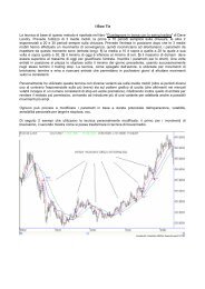
Grafico1
Evidente l’ottimo funzionamento dell’indicatore nelle fasi direzionali; la stessa situazione, tuttavia, la si
può verificare positivamente anche con l’adozione di una semplice media mobile esponenziale; come
detto sopra, tuttavia, usare una media comporta necessariamente la definizione di un parametro
temporale la cui scelta avrà carattere soggettivo o sarà legata alle aspettative di profitto del trader. Con
l’OTF il problema non si pone, ovviamente.

Grafici 2 e 3

Qui sopra si nota come, nelle fasi laterali, il numero di falsi segnali, a mio parere, non diminuisce in
misura tale da giustificarne in modo assoluto ed a carattere definitivo rispetto ad una media mobile (in
questo caso parametro 10, esponenziale). Infine, l’ultimo grafico mostra come, eventualmente,
l’indicatore potrebbe essere parte di una semplicissima metodologia di trading se accoppiato ad un
classico stocastico: si opera al ribasso con oscillatore stocastico in ipercomprato (al momento o di
recente) e chiusura della candela sotto l’indicatore OTF, viceversa al rialzo.
Sotto la spiegazione, completata dal codice in easy language per chi utilizzasse Tradestation.
INTRODUCTION
OPTIMAL TRACKING FILTERS
By
John Ehlers
Dr. R.E. Kalman introduced his concept of optimum estimation in 1960. Since that time, his technique
has proven to be a powerful and practical tool. The approach is particularly well suited for optimizing the
performance of modern terrestrial and space navigation systems. Many traders not directly involved in
system analysis have heard about Kalman filtering and have expressed an interest in learning more about
it for market applications. Although attempts have been made to provide simple, intuitive explanations,
none has been completely successful. Almost without exception, descriptions have become mired in the
jargon and state-space notation of the “cult”.
Surprisingly, in spite of the obscure-looking mathematics (the most impenetrable of which can be
found in Dr. Kalman’s original paper), Kalman filtering is a fairly direct and simple concept. In the spirit of
being pragmatic, we will not deal with the full-blown matrix equations in this description and we will be
less than rigorous in the application to trading. Rigorous application requires knowledge of the probability
distributions of the statistics. Nonetheless we end with practically useful results. We will depart from the
classical approach by working backwards from Exponential Moving Averages. In this process, we
introduce a way to create a nearly zero lag moving average. From there, we will use the concept of a
Tracking Index that optimizes the filter tracking for the given uncertainty in price movement and the
uncertainty in our ability to measure it.
SUB-OPTIMAL FILTERS
Tracking filters are used to estimate the position of a target using a linear model. Equation 1,
called an Alpha filter, shows that this model is comprised of using the previous estimate plus a constant
times the difference between the last real position and the last estimate.
X^ = X^[1] + (Z – X^[1])
Where X^ is the estimated next position
Z is the last real position
But this is exactly the same thing as the Exponential Moving Average (EMA) with which you are familiar. I
prefer to rearrange the terms so that the EMA is written as:
EMA = *Price + (1 – )*EMA[1]
As you know, this equation for the EMA produces a lag in the estimated price. We can improve our
estimate of position by adding an estimate of the velocity to the last known position in Equation 1.
Equation 1 then becomes:

X^ = X^[1] + ((Z + K*V^) – X^[1])
Where V^ is the velocity estimate
K is a gain factor
In general, the velocity estimate is an EMA of the rate of change of position, so that:
V^ = V^[1] + (V – V^[1])
This is the Beta part of an Alpha-Beta filter.
We can create a near zero lag filter for the special case where b = 1. In this case, equation 2 can
be written as:
ZEMA = *(Price + K*(Price – Price[4])) + (1 – )*ZEMA[1]
I took the liberty of using the four day “Momentum” (a misnomer if ever there was one) as the velocity
estimate. Figure 1 shows the EMA using = 0.25 compared to the ZEMA using the same alpha and K =
0.5. This is not a bad “zero lag” filter, even if it is sub-optimal.
MATHEMATICAL MODEL
Now that you are a little familiar with the model of target motion, the more general linear ideal
model is
y = y[1] + w[1]
where y[1] is the target state vector at time [1], is the state transition matrix, w[1] is the unknown target
maneuver, and is the maneuver/state transition matrix. The performance of the estimation process is
determined by the statistical characteristic of the estimation process. Since this system is linear and the
noise processes are assumed to be white, the optimal mean-squared-error is the Kalman filter. There are
errors in both the uncertainty of the maneuver and the uncertainty in the position measurement. Kalata 1
has introduced the concept of a Tracking Index, . He defines the Tracking Index as:
= (position maneuverability uncertainty) / (position measurement uncertainty)
We will return to the interpretation of the Tracking Index to price charts, but for now we will complete our
mathematical model. Given that is given, it implicitly specifies the optimal steady state solution.
Grinding through the math, the solution for the alpha filter is:
8)
We use the same alpha for an alpha-beta filter, and additionally have the relationship:
9)
α =
− Λ
2
4 2
( Λ + 16Λ
)
8
COMPUTING THE TRACKING INDEX
+
β =
2( 2 − α)
− 4 ( 1 − α)
1 Paul R. Kalata, “The Tracking Index: A Generalized Parameter for α−β and α−β−γ Target Trackers”,
IEEE Transactions on Aerospace and Electronic Systems”, Vol AES-20, No.2, March 1984, p 174-182

Under steady state conditions the position maneuverability uncertainty is just the bar-to-bar variation of
the mid range of the price bars. The measurement uncertainty is half the high-to-low range of the price
bar. Simple enough. As a practical matter, is it better to take the Exponential Moving Averages of these
two measurements to keep the Tracking Factor from going completely crazy. A smoothing constant of .2
results in reasonable a four bar lag 2 in both the numerator and denominator, fundamentally canceling lag
in the ratio. Therefore, the simplified equations for the Tracking Factor in terms of the price is:
A = .2*((H+L)/2 – (H[1]+L[1])/2) + .8*A[1]
B = .2*(H-L)/2 + .8*B[1]
= A / B
The EasyLanguage source code for an optimal tracking filter is given in SideBar1.
************************************** SideBar 1 *******************************************
EasyLanguage Code for an Optimal Tracking Filter
inputs: Price((h+l)/2);
vars: lambda(0),
alpha(0);
Value1 = .2*(Price - Price[1]) + .8*Value1[1];
Value2 = .1*(H - L) + .8*Value2[1];
if Value2 0 then lambda = AbsValue(Value1 / Value2);
alpha = ( -lambda*lambda + SquareRoot(lambda*lambda*lambda*lambda + 16*lambda*lambda)) /8;
Value3 = alpha*Price + (1-alpha)*Value3[1];
Plot1(Value3, "AlphaTrack");
2 John Ehlers, “Signal Analysis Concepts”