Analysis and Design of Sandwich Panels with Brittle Matrix ...

Vrije Universiteit Brussel 

Faculteit Toegepaste Wetenschappen 

Mechanica van Materialen en Constructies 

Pleinlaan 2, 1050 Brussel 

Analysis and Design of Sandwich Panels 

with Brittle Matrix Composite Faces 

for Building Applications 

ir. Heidi Cuypers 

Proefschrift ingediend voor het behalen van de graad van Doctor in 

de Toegepaste Wetenschappen 

Promotor: Prof. dr. ir. Jan Wastiels november 2001

Dankwoord 

Het is in de eerste plaats aan mijn promotor Prof. Jan Wastiels te danken dat dit 

werk onstaan is. De wekelijkse samenkomsten zijn dikwijls een goede motivatie 

geweest om verder te gaan en nieuw opgekomen vragen te bestuderen. Hij staat 

bekend, of beter gezegd berucht, als een kritische geest bij de studenten en heeft 

die reputatie alle eer aangedaan gedurende de vier jaar dat ik met hem heb 

gewerkt. Ondanks vele andere verplichtingen heeft hij toch de tijd weten te vinden 

voor een goede begeleiding. 

Myriam Bourlau en Agnes Vanaeken zorgden altijd voor snelle en goede 

administratieve ondersteuning en een schouderklopje op zijn tijd. Rene Heremans, 

Daniël Debondt en Gabriël Van den Nest zijn een grote hulp geweest in het 

praktische aspect van dit werk. Adri Vrijdag heeft voor enkele geslaagde foto’s 

gezorgd. Om de inbreng van Frans Boulpaep te beschrijven, komen woorden te 

kort. Zelden ben ik iemand met groter enthousiasme voor zijn werk en 

hulpvaardigheid ten opzichte van zijn collega’s tegengekomen. 

Gu Jun en Kurt De Proft zijn altijd zeer toffe bureaugenoten geweest. Jun heeft me 

op tijd en stond de humor van mijn werk laten inzien, ook al leek die soms ver 

weg. Net als Myriam en Agnes is ze dikwijls mijn grote zus geweest. Met Kurt 

heb ik fijne gesprekken gehad, zowel over het werk als over meer wereldse 

onderwerpen. Hem wens ik verder het allerbeste met de afwerking van zijn 

doctoraat. 

Jun, Joëlle, Jan, Joeri, Ronald, Kurt en Michaël hebben zich met veel moed door 

de soms nogal droge stof gewerkt om fouten op te sporen. Ik heb hier alle 

appreciatie voor. Gu Jun en Mazen Alshaer hebben in de laatste fase van dit werk 

een extra duwtje in de rug gegeven door hun medewerking in het uitvoeren van 

enkele experimenten. 

Verder hebben collega-assisten Kris Hoes, Jurgen Maes, Pascal Bouquet en Kim 

Croes gedurende drie of vier jaar voor een toffe werkomgeving gezorgd. Ik wens

hun ook het beste met de verderzetting van hun doctoraat of succes in hun nieuwe 

job. Ook de nieuwkomers Gunther, Georgios, Jan, Danniëlla en Shi wens ik succes 

met hun toekomstig onderzoek. 

Ik heb gedurende al die jaren veel steun gehad van mijn vader en Rie-Jeanne en 

mijn moeder en Karel. Mijn broer Stefan is dikwijls een rustpunt voor me geweest 

in de drukke schrijfperiode, ook al besefte hij het waarschijnlijk niet altijd. Ik 

wens hem en Isabelle het beste toe. Sommige personen van de oude garde en het 

nieuwe bloed binnen BEST-Brussel zijn me ook dierbaar gebleven of geworden. 

Enkele mensen die ik op Aero-Kiewit heb leren kennen, hebben de laatste twee 

jaren beduidend aangenamer gemaakt. Vrienden die ik al ettelijke jaartjes langer 

ken, hebben mijn vorderingen met interesse gevolgd: Frank, Ann, Geert, Aldo en 

Imogen, Bert, Wil, Maja, Joeri, Nico en Karen en Ronald. Vooral Ronald heeft me 

enorm gesteund. Een betere vriend kan je je jezelf niet toewensen. 

Heidi Cuypers, 

november 2001

Symbols and abbreviations 

Symbols concerning representative length scales 

. along 

. 

. 

. 

along < cs> 

. along ( su) 

. 

along ( su) 

N 

. alongδ 

0 

alongδ N 

along 

−2δ 

0 

f 

average of variable along 

average of variable along f 

average of variable along (su) 

average of variable along (su)N 

average of variable along δ0 

average of variable along δN 

average of variable along -2δ0 

Symbols concerning strain 

∆ε el elastic strain increment 

∆ε pl plastic strain increment 

∆εc 

composite strain variation 

∆εc elastic 

elastic term of composite strain variation 

∆εc slip slip term of composite strain variation 

∆εc zoneII extra composite strain term, due to multiple cracking 

composite strain variation, cycle N 

∆εc,N 

∆εc,N elastic elastic term of composite strain variation, cycle N 

∆εc,N repeat 

extra strain variation term, introduced by repeated loading 

∆εc,N slip slip term of composite strain variation, cycle N 

∆εf 

fibre strain variation 

∆εf elastic elastic term of fibre strain variation


∆εf slip slip term of fibre strain variation 

∆εf,N fibre strain variation, cycle N 

∆εf,N slip 

slip term of fibre strain variation, cycle N 

∆εm 

matrix strain variation 

εc 

composite strain 

εc max 

composite strain at maximum composite cycle stress 

εc min 

composite strain at minimum composite cycle stress 

εc thermal composite strain due to thermal load 

zone III 

εc 

εc zoneII εc,N 

composite strain after multiple cracking 

max εc,N 

maximum cycle strain, cycle N 

min minimum cycle strain, cycle N 

εc,x 

composite strain in zone III, ACK theory 

composite strain, measured in x-direction 

composite strain, measured in z-direction 

εc,z 

εexp(σj) experimental strain, at stress point σj 

εf 

εf,N max 

εm 

εm,x 

εm,z 

εmc 

fibre strain 

fibre strain at maximum composite stress, cycle N 

matrix strain 

matrix strain, measured in x-direction 

matrix strain, measured in z-direction 

composite multiple cracking strain 

ultimate matrix strain 

εmu 

εtheo(σj) theoretical strain, at stress point σj 

Symbols concerning stress 

∆σc 

composite stress variation 

∆σf 

fibre stress variation 

∆σf slip slip term of fibre stress variation 

matrix stress variation, cycle N 

∆σf,N 

∆σf,N slip slip term of fibre stress variation, cycle N 

∆σm matrix stress variation 

∆σm elastic elastic term of matrix stress variation 

∆σm slip slip term of matrix stress variation 

∆σm,N elastic elastic term of matrix stress variation, cycle N 

∆σm,N slip slip term of matrix stress variation, cycle N 

σ normal stress 

σ0 

initial failure stress (parameter in Weibull model) 

initial bending failure stress (parameter in Weibull model) 

σ0b

σc 

σc max 

σc min 

σcu 

σf 

σf,max 

σf,min 


composite stress 

maximum composite cycle stress 

minimum composite cycle stress 

composite failure stress 

fibre stress 

maximum stress in fibres 

minimum stress in fibres 

σf,N max fibre stress at maximum composite stress, cycle N 

σf,N min fibre stress at minimum composite stress, cycle N 

σfu 

σi 

σ y i- 

σ y i+ 

σij 

σ y ijσ 

y ij+ 

σj 

failure stress of the fibres 

normal stress in i-direction (i = x, y or z) 

normal yield stress in i-direction, compression (i = x, y or z) 

normal yield stress in i-direction, tension (i = x, y or z) 

shear stress in ij-plane (ij = xy, yz or xz) 

shear yield stress in ij-plane, negative sign (ij = xy, xz or yz) 

shear yield stress in ij-plane, positive sign (ij = xy, xz or yz) 

experimental stress point j 

matrix stress 

far field matrix stress (far from crack) 

σm 

σm ff 

σm ff,max 

far field matrix stress at maximum composite stress 

σm max matrix stress at maximum composite cycle stress 

σm thermal matrix stress due to thermal load 

σmax 

σmc 

σm,max 

σm,max max 

σm,min 

maximum stress 

composite multiple cracking stress 

maximum stress in matrix under static load 

maximum matrix stress at maximum composite stress 

minimum stress in matrix under static load 

σm,N ff,max far field matrix stress at maximum composite stress, cycle N 

σm,N max 

σm,N 

matrix stress at maximum composite stress, cycle N 

min 

σmu 

matrix stress at minimum composite stress, cycle N 

ultimate failure stress of the matrix 

σm,x matrix stress, measured in x-direction 

σnom nominal stress 

σR 

reference failure stress (parameter in Weibull model) 

σRb 

reference bending failure stress (parameter in Weibull model) 

σwr 

wrinkling stress 

τ shear stress 

frictional matrix-fibre interface shear stress, first loading 

τ0 

τ0 x shear stress component along x-axis 

τ0sf 

single fibre frictional matrix-fibre shear stress

τa 

τau 

τd0 

τi0 

τN 

τu 

Other symbols 


adhesion matrix-fibre shear bond 

adhesion matrix-fibre shear bond strength 

dynamic frictional shear stress (matrix-fibre interface) 

frictional shear stress (matrix-fibre interface) 

frictional matrix-fibre interface shear stress, cycle N 

ultimate shear stress 

α matrix / fibre stiffness ratio of the composite 

αf 

thermal expansion coefficient of the fibres 

αm 

thermal expansion coefficient of the matrix 

βl 

variable used to calculate fibre length efficiency factor 

δt time increment 

δ0 

Matrix-fibre debonding length at first loading 

δf 

length along which normal stresses are transferred to fibres 

δN 

debonding length, cycle N 

∆T temperature difference 

γG 

safety coefficient on permanent load 

γQ 

safety coefficient on variable load 

ηθ 

orientation efficiency factor 

ηl 

length efficiency factor 

ηlev 

parameter in Largest extreme value probability distribution 

ϕcot 

creep coefficient of the core 

µi 

snow shape coefficient 

µlev 

parameter in Largest extreme value probability distribution 

µlog 

parameter in Lognormal probability distribution 

νm 

Poisson’s ratio of the matrix 

νfxz 

Poisson’s ratio of the fibres 

νxz 

Poisson’s ratio of the composite 

θ local cylindrical coordinate 

θx 

angle between fibre and x-axis 

ρ local cylindrical coordinate 

ρf 

density of glass fibres 

σlog 

parameter in Lognormal probability distribution model 

ω matrix-fibre interface degradation parameter 

ψ0,i 

combination coefficient 

ψ1,i 



ψ2,i


A constant, concerning contribution of term(s) to bending stiffness 

Ac 

composite section, transverse to the loading direction 

Aexposed exposed bundle surface area 

Af 

Af 

fibre section (Af = VfAc) 

* equivalent fibre section 

Am 

matrix section (Am=VmAc) 

Atotal total bundle surface area 

b width 

average crack spacing 

f average crack spacing at the end of matrix multiple cracking 

C1 constant in formulation of interface degradation parameter 

C2 constant in formulation of interface degradation parameter 

cd 

dynamic coefficient (wind load) 

ce 

exposure coefficient (snow load) 

cpe 

external pressure coefficient (wind load) 

cpi 

internal pressure coefficient (wind load) 

ct 

thermal coefficient (snow load) 

D bending stiffness of sandwich panel 

Df 

sum of the separate flexural rigidities of the faces 

DQ 

shear stiffness of the core 

e distance between the centroid of the core and the neutral axis 

Ec 

composite stiffness 

Ec1 

composite stiffness as determined by the rule of mixtures 

Ec3 

experimental obtained composite stiffness in post-cracking zone 

Eco 

E-modulus of core 

Ecycle linearised stiffness of one loading-unloading stress-strain cycle 

Ecycle,N linearised stiffness, cycle N 

E el 

elastic stiffness 

Ef 

E-modulus of fibre 

Efa 

E-modulus of face 

Ef b stiffness of lower face (bottom) 

Ef t stiffness of upper face (top) 

Ei,+ pl 

plastic stiffness in i direction, tension (i = x, y or z) 

Ei,+ pl plastic stiffness in i direction, compression (i = x, y or z) 

Ei, el elastic stiffness in i direction (i = x, y or z) 

Em 

E-modulus of matrix 

E pl 

plastic stiffness 

E T 

tangent stiffness 

F cumulative distribution function 

f probability distribution function


F x external external applied force parallel with the x-axis 

F x fibre total force in the x-direction taken by all fibres 

F x matrix total force in the x-direction, taken by the matrix 

F y external external applied force parallel with the y-axis 

F y fibre total force in the y-direction taken by all fibres 

F y matrix total force in the y-direction, taken by the matrix 

Gco 

shear modulus of the core 

Gij el 

elastic shear modulus ij plane (ij = xy, xz or yz) 

Gij pl 

plastic shear modulus ij plane (ij = xy, xz or yz) 

Gk 

permanent load 

Gm 

shear modulus of the matrix 

h height of specimen 

K efficiency factor in post-cracking zone 

Ku 

unloading efficiency factor 

l length of specimen 

L span of sandwich panel 

lf 

length of fibre 

m Weibull modulus (parameter in Weibull model) 

Mb 

moment in lower face (bottom) 

Mt 

moment in upper face (top) 

N number of applied load cycles 

Nb 

normal force in lower face 

Nexp number of experimental points in considered stress interval 

Nfb 

number of fibres in a bundle 

Nfibres number of fibres in a composite section 

nfl 

number of fibre layers 

Nt 

normal force in upper face 

P probability 

p pressure load on sandwich panel 

Pfibre force taken by one fibre 

P x fibre force in the x-direction taken by one fibre 

P y fibre force in the y-direction taken by one fibre 

qk 

characteristic wind load pressure 

Qk 

variable load 

Qk1 

variable load with largest effect 

Qk2 

other variable loads 

r fibre radius 

R radius of matrix around the fibre 

Rav 

ratio of average composite strains in two transverse directions 

rotz 

rotation around the z-axis


s snow load pressure on panel 

(su) unloading slip length 

(su)N unloading slip length, cycle N 

Sd 

equivalent static load, used for design 

sk 

characteristic snow pressure on the ground 

t time 

T0 x 

frictional shear flux along the x-axis 

t1 

initial time 

tc 

thickness of laminate or specimen 

tc 

thickness of core 

tf b lower face thickness (bottom) 

tf t upper face thickness (top) 

Tinside temperature inside building 

Toutside temperature outside building 

ub 

displacement of lower face (x-direction) 

uc 

displacement of core (x-direction) 

ut 

displacement of upper face (x-direction) 

ux 

displacement in the x-direction 

uy 

displacement in the y-direction 

V volume 

Vb 

shear force in lower face 

Vf 

fibre volume fraction 

Vf * 

equivalent fibre volume fraction 

Vfb 

volume fraction of fibres in a bundle 

Vf crit 

critical fibre volume fraction 

Vm 

matrix volume fraction 

VR 

reference volume 

Vt 

shear force in upper face 

w width of specimen 

w wind load pressure on panel (Chapter 7) 

wb 

displacement of lower face (y-direction) 

wfibrelayer weight of fibre layer (mat or weave) per m² 

wt 

displacement of upper face (y-direction) 

X general variable 

local cylindrical coordinate 

xl

Abbreviations 


ACK Aveston-Cooper-Kelly model 

CDF cumulative distribution function 

CLC characteristic load combination 

TMA thermomechanical analyser 

EST elementary sandwich theory 

FEM finite element method 

FLC frequent load combination 

IPC inorganic phosphate cement 

LEV largest extreme value model 

LSC least square coefficient 

LVDT linear variable differential transducer 

ncore number of element divisions across height of a core 

ndiv number of element divisions along length of a sandwich panel 

nface number of element divisions across height of a face 

PDF probability distribution function 

QLC quasi-permanent load combination 

SEV smallest extreme value model 

SLS serviceability limit state 

UD unidirectional reinforcement 

ULS ultimate limit state

Dankwoord 


Table of contents 


Chapter 1: Introduction 1 

1.1 Research context 1 

1.2 Objectives of the thesis 2 

1.3 Basic assumptions in this thesis 3 

1.4 Outline of the thesis 4 

1.5 References 6 

Chapter 2: IPC composite specimens under monotonic loading 9 

2.1 Introduction 9 

2.2 Materials 10 

2.2.1 E-glass fibres as reinforcement 10 

2.2.2 matrix material: Inorganic Phosphate Cement (IPC) 10 

2.2.3 E-glass fibre reinforced IPC laminates 11 

2.3 IPC laminates under compressive loading 12 

2.3.1 introduction 12 

2.3.2 test set-up 12 

2.3.3 materials and results 13 

2.3.4 discussion and conclusions 15 

2.4 Tensile behaviour of continuous UD-reinforced IPC 17 


2.4.2 basic assumptions 17 

2.4.3 formulation of the ACK theory 19 

2.4.3.1 zone I 19 

2.4.3.2 zone II 20 

2.4.3.3 zone III 25 

2.4.4 points of discussion in the ACK theory 26 

2.4.5 the statistical nature of the IPC matrix tensile strength 28 

2.4.6 the Weibull probability distribution 32


2.4.7 formulation of the stochastic cracking theory 34 

2.4.7.1 formulation when > 2δ0 

36 

2.4.7.2 formulation when < 2δ0 

37 

2.4.7.3 σc at which > 2δ0 becomes < 2δ0 

38 

2.4.8 experiments on UD-reinforced IPC specimens 38 

2.4.8.1 specimens 38 

2.4.8.2 ACK model versus experimental results 39 

2.4.8.3 stochastic cracking model versus experimental results 40 

2.4.8.4 ACK model versus stochastic cracking model 45 

2.5 Tensile behaviour of 2D-randomly reinforced IPC 46 


2.5.2 derivation of the ACK based model 47 

2.5.2.1 linear elastic zone or pre-cracking zone (zone I) 47 

2.5.2.2 post-cracking zone (zone III) 48 

2.5.2.3 multiple cracking zone (zone II) 50 

2.5.3 derivation of the stochastic cracking based model 53 


53 


53 

2.5.4 experiments on 2D-randomly reinforced IPC specimens 54 

2.5.4.1 specimens 54 

2.5.4.2 ACK based model versus experimental results 54 

2.5.4.3 stochastic cracking based model versus experimental results 55 

2.5.4.4 ACK based model versus stochastic cracking based model 56 

2.6 Tensile behaviour of IPC composite specimens: discussion and conclusions 57 

2.7 Evolution of matrix stresses transverse to the loading direction 58 

2.7.1 theoretical derivation of the Poisson’s ratio based on the ACK theory 59 

2.7.2 experimental verification 61 

2.8 Experimental determination of the shear modulus of IPC composite specimens 63 

2.8.1 specimens and test set-up 63 

2.8.2 results 64 

2.9 Conclusions 65 


Chapter 3: Unloading of IPC composite specimens 71 


3.2 Definitions and assumptions 71 

3.3 ACK (based) theory for unloading 73 


3.3.2 derivation of the linearised E-modulus of a cycle: Ecycle 

3.3.2.1 partial matrix-fibre slip during unloading 73 

3.3.2.2 from partial to total matrix-fibre slip 76 

3.3.2.3 total matrix-fibre slip during unloading 76 

3.4 stochastic cracking (based) theory for unloading 77 

73



3.4.2 derivation of linearised E-modulus of a cycle: Ecycle 

78 

3.4.2.1 partial matrix-fibre slip during unloading 78 

3.4.2.2 from partial to full matrix-fibre unloading slip, > 2δ0 80 

3.4.2.3 from partial to full unloading matrix-fibre slip, < 2δ0 83 

3.4.2.4 total matrix-fibre slip during unloading 83 

3.5 IPCstress-strain.exe: a program to predict unloading 85 

3.6 Experiments 86 

3.6.1 test set-up and materials 86 

3.6.2 test results 87 

3.6.3 unloading behaviour as predicted by the ACK based model 88 

3.6.4 unloading behaviour as predicted by the stochastic cracking based 93 

3.6.5 ACK based model versus stochastic cracking based model 94 



Chapter 4: IPC Composite specimens under repeated tensile loading 99 


4.2 Theoretical derivation: general remarks 100 


4.2.2 assumptions and definitions 101 

4.3 Theoretical derivation of a fatigue theory from the ACK (based) model 103 

4.3.1 evolution of εc,N max with N 103 

4.3.2 evolution of Ecycle,N with N 106 

4.3.2.1 partial matrix-fibre unloading slip 106 

4.3.2.2 when partial becomes total matrix-fibre slip 108 

4.3.2.3 total matrix-fibre unloading slip 108 

4.4 Theoretical derivation of a fatigue theory from the stochastic cracking (based) 109 

4.4.1 evolution of εc,N max with N 110 

4.4.1.1 crack spacing exceeds twice the debonding length 110 

4.4.1.2 transition from >2δN to < 2δN 

111 

4.4.1.3 crack spacing smaller than twice the debonding length 112 

4.4.2 evolution of Ecycle,N with N 112 

4.4.2.1 partial matrix-fibre unloading slip 112 

4.4.2.2 partial to total matrix-fibre unloading slip, > 2δN 112 

4.4.2.2 partial to total matrix-fibre unloading slip, < 2δN 113 

4.4.2.4 total matrix-fibre unloading slip 113 

4.5 Determination of interface wear evolution from experimental observations 113 


4.5.2 ACK (based) theory 114 

4.5.3 stochastic cracking (based) theory 114 

4.5.4 ACK (based) theory versus stochastic cracking (based) theory 114 

4.6 Testing program 115


4.7 UD-reinforced IPC composite specimens under repeated loading 116 


4.7.2 material properties and test schedule 116 

4.7.3 determination of material properties 116 

4.7.4 results under repeated loading 117 

4.7.5 determination of interface degradation parameter from test results 118 


4.8 UD-reinforced IPC composite specimen under limited repeated loading 122 





4.8.5 determination of interface degradation parameter from test results 124 

4.8.6.1 extrapolation from limited cycling to high number of cycles 124 

4.8.6.2 repeated loading at lower maximum cycle stress 128 

4.9 UD-reinforced IPC composites under repeated loading: discussion 130 

4.10 2D-randomly reinforced IPC composite specimens under repeated loading 131 





4.10.5 theoretical versus experimental degradation behaviour 135 

4.10.5.1 results 135 

4.10.5.2 specimens cycled up to 22 or 27.5MPa: discussion 135 

4.10.5.3 specimens cycled up to 11 or 16.5MPa: discussion 136 

4.10.5.4 specimens cycled up to 6MPa: discussion 137 


4.11 Interpretation of hysteresis 139 


4.12.1 conclusions from tests on UD-reinforced specimens 140 

4.12.2 conclusions from tests on 2D-randomly -reinforced specimens 141 


Chapter 5. Sandwich modelling 143 


5.2 Sandwich modelling: overview 143 

5.2.1 single layer theories 144 

5.2.2 layer-wise theories 144 

5.2.3 predictor-corrector and hierarchical modelling theories 145 

5.3 A 2D-continuum approach: plane stress versus plane strain 145 

5.4 Sandwich panels under monotonic loading: the use of ANSYS 146 


5.4.2 implementation of material behaviour 146


5.4.2.1 implementation of material behaviour: ‘multilinear elastic’ 146 

5.4.2.2 implementation of material behaviour: ‘aniso’ 147 

5.4.3 type of model: discussion 150 

5.4.3.1 elementary sandwich theory 150 

5.4.3.2 advanced sandwich theory 153 

5.4.4 parameters of study 155 

5.4.5 a reference sandwich beam 156 

5.4.6 comparison of models: results and discussion 158 

5.4.7 influence of span 160 

5.5 The behaviour of sandwich panels during unloading and repeated loading 163 



Chapter 6: Experimental work on sandwich panels 169 


6.2 Strength of the core-face interface 169 

6.2.1 failure in tension 169 

6.2.2 shear failure 170 

6.3 Large-span sandwich panels: materials and geometry 172 

6.3.1 face materials 172 

6.3.2 core material 172 

6.3.3 geometry 172 

6.4 Panels with 2m span: test set-up 173 

6.5 Panels with 2m span: results 174 

6.6 2m span panels: theoretical predictions versus experimental results 176 

6.6.1 face properties of the tested panel 176 

6.6.2 theoretical prediction of the load-displacement behaviour 178 

6.6.3 theoretical versus experiments: initial loading up to 2/3 rd of maximum 179 

6.6.3.1 load-displacement curves 179 

6.6.3.2 load-strain curves 180 

6.6.4 theory versus experiments: initial unloading from 2/3 rd of maximum 182 

6.6.5 theory versus experiments: repeated loading up to 2/3 rd of maximum 183 

6.6.6 theory versus experiments: loading to maximum load 185 

6.7 Short-span panels: geometry and test set-up 186 

6.7.1 geometry and test set-up 186 

6.7.2 reliability of strains, measured by strain gauge laminated into a face 188 

6.8 Short-span panels: results 189 

6.8.1 loading up to 1/3 rd of maximum load: results 190 

6.8.2 loading up to 2/3 rd of maximum load: results 191 

6.9 Short-span panels: theoretical FEM predictions versus experimental results 192 

6.9.1 properties of the faces of the tested panels 192 

6.9.2 theory versus experiments: initial loading up to 1/3 rd of maximum 193 

6.9.3 theory versus experiments: initial loading up to 2/3 rd of maximum 193




Chapter 7: Design of sandwich panels with IPC composite faces 197 


7.2 Design methodology 198 

7.2.1 wind load 198 

7.2.2 snow load 199 

7.2.3 temperature load 199 

7.2.4 own weight 199 

7.2.5 combination of loads 199 

7.5.2.1 ultimate limit state (ULS) 200 

7.5.2.2 serviceability limit state (SLS) 202 

7.5.2.3 SLS: frequent load combination (FLC) 202 

7.5.2.4 SLS: characteristic load combination (FLC) 204 

7.2.6 design of sandwich panels with IPC faces 205 

7.3 Materials and modelling 206 

7.3.1 materials properties 206 

7.3.2 thermal expansion of UD-reinforced IPC 206 

7.4 Case studies 209 

7.4.1 case study 1: flat wall panel 209 

7.4.2 case study 2: flat roof panel 209 

7.4.3 case study 3: flat roof panel with intermediate support 209 

7.4.4 modelling and design 209 

7.5 Design under frequent and characteristic load combination (SLS) 210 




7.5.4 conclusions 214 

7.6 Design in ultimate limit state 210 





7.7 Design in under FLC after unloading from CLC 216 






7.8 Design under repeated loading 


7.8.2 case study 1: flat wall panel 220





7.9 Comparison of sandwich panels with IPC composite and steel faces 225 


7.9.2 comparison of solutions 225 




Chapter 8: Conclusions 229 

8.1 Conclusions on the behaviour of IPC composite specimens 229 

8.2 Conclusions on sandwich modelling 231 

8.3 Conclusions on design criteria for sandwich panels with IPC faces for building 233 

8.4 Future research topics 234 

Appendix 1: Probability distribution functions 

Appendix 2: Probability plotting 

Appendix 3: Hysteresis 

Appendix 4: Macro for implementation of unloading 

Appendix 5: Macro for implementation of repeated loading

Chapter 1 

1.1 Research context 

Introduction 

Sandwich panels were first used in aircraft industry. The combination of metal 

membrane skins and honeycomb cores leads to rather stiff lightweight structures. 

Only more recently sandwich panels have been introduced as wall cladding panels 

and as roof panels. The materials, which are used most for this type of application, 

are two steel faces and a cellular core, which also functions as thermal insulation. 

Other material combinations are possible, but diversity in materials in sandwich 

panels for housing is still not common practice. 

Apart from sandwich elements, the use of composite materials in buildings has 

been the subject of numerous studies. Ferrocements are a good example of the 

potential of composite materials in construction of buildings. The advantages of 

ferrocements are: relatively low cost, availability of the basic components, fireretarding 

properties and easy production. The use of ferrocements also ensures 

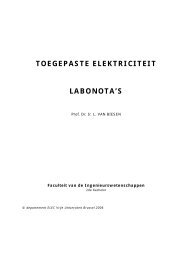
large flexibility in design. The concept of “housing” can be interpreted as the 

future house owner desires, as illustrated in figure 1.1. 

Figure 1.1: house structures using ferrocement shells (Naaman, 2000) 

1

Chapter 1: Introduction 

The use of ferrocement composites and of sandwich panels reduces construction 

time and energy. Lightweight construction elements are less likely to endanger the 

life of people in case of collapse, for example due to an earthquake. Moreover, 

lightweight constructions are more resistant to earthquakes than solid 

constructions. “A house, constructed mainly with lightweight panels may entrap 

people when it breaks down. However, the probability of suffering serious injuries 

or death decreases, due to the reduced weight of the collapsed elements.“ 

(Goldsworthy, 2000) 

A new material, Inorganic Phosphate Cement (IPC), has been developed at the 

‘Vrije Universiteit Brussel’. After hardening, the IPC material properties are 

similar to those of cement-based materials. IPC is a two-component system, 

consisting of a calcium silicate powder and a phosphate acid based solution of 

metaloxides. One of the major benefits of IPC, when compared to other existing 

cementitious materials, is the non-alkaline environment after hardening. Due to 

this, ordinary E-glass fibres are not attacked by the matrix and can be used as 

reinforcement. Therefore, E-glass fibre reinforced IPC is a cementitious 

composite, allowing production of very thin and cost-effective laminates. A 

combination of the application of this type of cementitious composite and 

sandwich panels is discussed in this work. 

1.2 Objectives of the thesis 

Nowadays, numerous projects, which make use of brittle matrix composites, are 

under investigation. At present, the production of cost-effective cementitious 

composites with alkali resistant glass fibres is not achievable. Since IPC is 

compatible with cheaper E-glass fibres, industrial production of a new type of 

construction elements becomes feasible. Indeed, one of the possible applications 

of these thin cementitious laminates is their implementation as faces in a sandwich 

panel. To the author’s knowledge, the use of very thin cementitious faces in 

sandwich panels for building applications has not been subject of profound study 

up till now. 

In the first part of this thesis, focus is put on the behaviour of E-glass fibre 

reinforced IPC laminates. Loading, unloading and repeated loading is discussed. 

The behaviour of unidirectionally reinforced IPC under monotonic tensile loading 

and limited repeated loading has been the subject of study before (Bauweraerts, 

1998). The behaviour of 2D-randomly reinforced IPC specimens under monotonic 

tensile loading has been studied by Gu et al. (1998). Refinements on the models, 

discussed by Bauweraerts (1998) and Gu et al. (1998), are introduced in this 

thesis. The behaviour of unidirectionally or 2D-randomly reinforced IPC under 

monotonic loading, unloading and repeated loading is also tested and discussed in 

2


this thesis. Publications on the behaviour of ceramic matrix composites (Curtin et 

al., 1998; Rouby and Reynaud, 1992; Evans et al., 1992) are used as references for 

the formulation of a theory, describing the behaviour of IPC composite specimens. 

The second part of this thesis provides an extensive report on the analysis and 

design of lightweight panels with thin cementitious composite faces as roof and 

wall cladding panels. The most interesting features of wall and roof panels are 

thermal and acoustical insulation, mechanical resistance, fire resistance and 

resistance against environmental actions such as humidity changes, UV radiation 

and freezing-thawing cycles. Especially, the analysis of sandwich panels under 

mechanical loading is discussed in this work. The feasibility of load bearing 

sandwich roof or wall panels with cementitious faces depends on the initial 

stiffness and strength properties and their evolution as a function of time, 

environment, etc. The design philosophy is based on the Preliminary 

Recommendations for Sandwich Panels (ECCS, 1991) and the Updated 

Recommendations for Sandwich Panels (Berner et al., 2000). However, these 

recommendations have been formulated with the specific behaviour of sandwich 

panels with steel faces in mind. In this work, the applicability of these 

recommendations is studied for sandwich panels with IPC composite faces. 

Several sandwich design modifications, which are necessary, are introduced. 

Finally, the load bearing capacity of sandwich panels with IPC faces is compared 

to the capacity of more classical sandwich panels with steel faces. 

1.3 Basic assumptions in this thesis 

In this work, sandwich panels are assumed to work as wide beams rather than as 

plates. Roof and wall sandwich panels are usually mounted to the main structure at 

two opposite ends. Since practically all applied loads are either pressure loads or 

line loads along the width of the sandwich panel, a wide beam approach is 

legitimised. Point loads are not considered in this work. 

The sandwich element should be able to sustain a combination of several loads. 

The loads considered in this work are: 

1. own weight, which is a permanent dead load 

2. snow load, which is a variable free action 

3. wind load, which is a variable free action 

4. temperature, which is a variable free action 

Before any analysis is made, the desired lifetime of the structure should be 

determined. Table 1.1 presents a general classification of structures and the 

lifetime they should survive without any major repair (Eurocode 1). 

3


The Preliminary Recommendations for Sandwich Panels advise a lifetime of 50 

years. Sandwich panels used as roof or wall elements are thus structures of type 3, 

according to table 1.1. This work assumes a desired lifetime of 50 years. 

Table 1.1: classification of structures as function of their lifetime (Eurocode 1) 

classification lifetime (years) example 

1 1 - 5 temporary structures 

2 25 removable structural elements 

3 50 buildings 

4 100 civil engineering 

Both the ultimate limit state and the serviceability limit state are considered in the 

design of sandwich panels for building purposes. An important serviceability limit 

state is based on the limitation of the maximum deflection. In the Preliminary 

Recommendations for Sandwich Panels and the Updated Recommendations for 

Sandwich Panels, several propositions are made on this limitation. The proposed 

limits are 1/100 th , 1/200 th or 1/300 th of the span. In this work the maximum 

allowed deflection is 1/200 th of the span. 

1.4 Outline of the thesis 

Prior to any analysis of a construction element, the mechanical properties of all 

materials must be obtained. 

Polymer foams are suitable core materials and will be used in this study. They are 

less expensive than honeycomb cores. Polymer foam cores provide good thermal 

insulation and satisfactory mechanical stiffness and strength, all of which are a 

function of their density. The stress-strain behaviour of polymer foams has been 

discussed extensively in literature and is well known. 

The modelling of the behaviour of E-glass fibre reinforced IPC under monotonic 

loading is discussed in Chapter 2. Since the faces in a sandwich panel are mainly 

loaded in tension or in compression, the behaviour of E-glass fibre reinforced 

specimens under these types of loads is discussed. The assumption of linear elastic 

behaviour of E-glass fibre reinforced IPC in compression is checked 

experimentally. However, the stress-strain behaviour of E-glass fibre reinforced 

IPC laminates under tensile loading is non-linear. Constitutive modelling of Eglass 

fibre reinforced brittle matrix composites under monotonic tensile loading is 

also presented in Chapter 2. The presented theoretical constitutive models are 

formulated from meso-mechanical phenomena in the composite. The theoretical 

stress-strain behaviour is compared with experimental results on unidirectionally 

and 2D-randomly reinforced specimens. 

4


The meso-mechanical modelling philosophy applied for loading is used as basic 

theory to predict the unloading behaviour of E-glass fibre reinforced IPC 

laminates. The theoretical prediction of the unloading stress-strain behaviour of 

IPC composite specimens is discussed in Chapter 3. Experimental data obtained 

on unidirectionally reinforced IPC specimens and on 2D-randomly reinforced 

specimens are compared with these theoretical predictions. 

The phenomena leading to fatigue failure in composites are completely different 

from those of conventional materials. Whereas fatigue failure occurs from the 

initiation and propagation of one single crack for most conventional materials, 

several damage mechanisms can interact and lead to final failure under repeated 

loading of E-glass fibre reinforced IPC. Apart from fatigue failure, accumulation 

of deformations under repeated loading might be rather large for the studied type 

of composites. Understanding the meso-mechanics in E-glass fibre reinforced IPC 

laminates under cyclic tensile loading is thus essential. These phenomena are 

discussed in Chapter 4. Damage types to be considered are: matrix cracking, fibre 

failure, fibre pull-out and matrix-fibre interface degradation. The relative 

importance of a degradation mechanism is function of fibre volume fraction, type 

of fibre reinforcement, average stress and stress amplitude. The importance of 

damage mechanisms in IPC composite specimens is discussed in Chapter 4 and 

verified experimentally. A theoretical meso-mechanical based model is discussed. 

Various sandwich models are presented in Chapter 5. Their efficiency in analysis 

and design of sandwich panels with cementitious composite faces is discussed. 

The use of a material with non-linear stress-strain behaviour makes it extra 

challenging to determine whether a simplified model gives appropriate predictions 

of deflections and internal stresses, once the tensile face is subjected to multiple 

cracking. Guidelines on an efficient practical use of the presented sandwich 

models are discussed and illustrated. The introduction of the material behaviour of 

E-glass reinforced IPC in the finite element models is also discussed in Chapter 5. 

Small and larger scale sandwich panel testing is presented and discussed in 

Chapter 6. Since the controlled introduction of a pressure load on panels in the 

laboratory is difficult, the panels are subjected to a four point bending test. This 

type of loading is not experienced in situ, but it provides a useful benchmark. It is 

discussed whether the presented sandwich models indeed provide a useful and 

accurate prediction tool for stresses, strains and displacements of sandwich panels 

with IPC composite faces. The panels are subjected to monotonic loading, 

unloading and repeated loading. Correspondence of experimental and theoretical 

load-deflection curves and load-strain curves of several sandwich panels is 

discussed. 

5


Modifications might be necessary when the design rules for classical sandwich 

panels with steel faces are used for sandwich panels with IPC composite faces. 

These modifications are presented and discussed in Chapter 7. Several case 

studies illustrate the design philosophy of sandwich panels with IPC composite 

faces. It is illustrated in Chapter 7 that the modelling of the face behaviour under 

various loading conditions is a conditio sine qua non for the analysis and design of 

sandwich panels with IPC composite faces for construction purposes. Finally, the 

load bearing capacity of sandwich panels with IPC composite faces is compared 

with the capacity of classical panels with steel faces. 

The main conclusions of this thesis are summarised in Chapter 8. 

1.5 References 

P. Bauweraerts, Aspect of the Micromechanical Characterisation of Fibre 

Reinforced Brittle Matrix Composites, Phd. thesis, VUB, 1998 

K. Berner, J.M. Davies, P. Hassinen, L. Heselius, Updated European 

recommendations for sandwich panels, Proceedings 5 th International Conference 

on Sandwich Construction, EMAS Publishing, Sept 5-7, 2000, pp.389-400 

W.A. Curtin, B.K. Ahn, N. Takeda, Modeling Brittle and Tough Stressstrain 

Behaviour in Unidirectional Ceramic Composites, Acta mater., No. 10, 

1998, pp.3409-3420 

ECCS publication, Preliminary European Recommendations for Sandwich 

Panels, part I, Design, Technical Committee 7, Working Group 7.4, 1991 

Eurocode 1, Grondslag voor ontwerp en belastingen op draagsystemen 

A.G. Evans, F.W. Zok, R.M. McMeeking, Fatigue of ceramic matrix 

composites, Acta metallurgica et materialia, 43, 1995, pp.859-875 

J. Gu, X. Wu, H. Cuypers and J. Wastiels, Modeling of the tensile 

behaviour of an E-glass fibre reinforced phosphate cement, Computer Methods in 

Composite Materials VI, proceedings CADCOMP 98, 1998, pp.589-598 

A.E. Naaman, Ferrocement & laminated cementitious composites, Techno 

Press 3000, 2000 

6


D. Rouby and P. Reynaud, Fatigue behaviour related to interface 

modification during load cycling in ceramic-matrix fibre composites, Composite 

Science and Technology, 48, 1993, pp.109-118 

W. B. Goldsworthy, Composite Housing - why isn’t it here today?, 

Composites Technology, March/April 2000, pp.13 

7

Chapter 2 

2.1 Introduction 

IPC composite specimens 

under monotonic loading 

The material properties of pure IPC matrix and E-glass fibres are presented in this 

chapter. These properties are used in the formulation of the theory describing the 

behaviour of E-glass fibre reinforced specimens under monotonic compressive, 

tensile and shear loading. External tensile and compressive loads on the specimens 

are applied along one loading-axis: the x-axis. 

It is verified experimentally that E-glass fibre reinforced IPC specimens under 

compression show a linear elastic stress-strain relationship until failure. 

The stress-strain curves obtained from tensile testing are more complex due to 

non-linear irreversible micro- or meso-mechanical events. Unloaded specimens, 

which were subjected to tension, inevitably show residual strains and internal 

residual stresses. Two models, providing a prediction method of the stress-strain 

behaviour of IPC composite specimens in tension, are presented and discussed in 

this chapter. The goal to be achieved in this chapter is the formulation of a model 

based on physical micro- or meso-mechanical phenomena. However, the model 

should still be simple enough for analytical prediction of the macro-mechanical 

behaviour of a IPC composite. The theoretical stress-strain curve predictions are 

compared with experimental curves on unidirectionally reinforced and 2Drandomly 

reinforced specimens. 

The compressive and tensile stress-strain formulations, obtained in this chapter, 

are implemented later as constitutive equations in finite element calculations of 

sandwich panels with E-glass fibre reinforced IPC faces. 

9

Chapter 2: IPC composite specimens under monotonic loading 

Even though the theoretical stress-strain relationship of IPC laminates under shear 

is not discussed fundamentally, experimental results obtained from torsion testing 

are presented and discussed in this chapter. 

2.2 Materials 

Knowledge of the material properties of the different components is a minimum 

requirement for a proper description of the behaviour of E-glass fibre reinforced 

IPC composites. All IPC composite specimens in this chapter are fabricated as 

described here, unless mentioned otherwise explicitly. 

2.2.1 E-glass fibres as reinforcement 

Two types of E-glass fibre reinforcements are used: chopped glass fibre mats 

(“2D-random”) with a fibre density of 300g/m² (Owens Corning MK12) and 

quasi-unidirectional woven roving (“UD”) with a fibre density of 158g/m². 

141g/m² of fibres are present as reinforcement in the main direction and 17g/m² of 

the reinforcement is aligned along the transverse direction (Syncoglas Roviglas 

R17/141). The fibre diameter is 14µm for all fibres. The unidirectional fibres are 

continuous fibres. The length of the chopped fibres is 50mm. The E-glass fibre 

reinforcement consists of fibre bundles rather than of single fibres. The number of 

fibres per bundle is ±1500 for the UD-reinforcement and ±540 for the 2D-random 

reinforcement. Properties of the E-glass fibres are listed in table 2.1. 

Table 2.1: properties E-glass fibres, found in literature and used in this work 

density 

(kg/m ³ tensile Young’s thermal 

strength modulus expansion 

) (MPa) (GPa) (10e -6 ) 

Chawla (1993) 2550 1750 70 4.7 

Bentur and Mindess (1990) 2540 3500 72.5 - 

Matthews and Rawlings (1994) 2540 2200 70 - 

used in this work 2540 1700 72 4.7 

2.2.2 matrix material: Inorganic Phosphate Cement (IPC) 

Inorganic phosphate cement (IPC) has been developed at the ‘Vrije Universiteit 

Brussel’. IPC is a two-component system, consisting of a calcium silicate powder 

and a phosphate acid based solution of metaloxides. After hardening, the IPC 

material properties are similar to those of cement-based materials. Although the 

strength in compression is rather high, the tensile strength is low. The tensile 

strength of a IPC specimen is about one tenth of the compressive strength. Like 

ceramic or cementitious materials, IPC shows a high temperature resistance and 

good fire retarding properties. Since all basic components are inorganic, no toxic 

gasses are released in case of fire hazard. 

10


One standard IPC mixture is chosen in this work, without use of any fillers or 

retarding or accelerating components. The powder component is called N2 and the 

liquid mixture is noted by B23. More details cannot be given for reason of 

confidentiality (PCT patent application: WO 97/19033). The weight ratio of 

powder to liquid, used for all IPC mixtures in this work, is 1/1.25. 

IPC laminates or blocks are cured in ambient conditions for 24 hours. Post-curing 

is performed at 60°C for 24 hours. Like most cementitious mixtures, the strength 

of IPC increases with time. This effect can however be accelerated by the postcuring 

at 60°C. Typical values of stiffness, strength and own weight can be found 

in table 2.2. The presented stiffness and strength properties are average values. 

Variations on these values are mentioned if necessary. After cutting, the 

specimens are dried in ambient conditions, unless mentioned otherwise. 

Table 2.2: properties of the IPC matrix; after Gu et al. (1998), Bauweraerts (1998b) and Cuypers 

et al. (2000) 

tensile strength compressive strength E-modulus own weight 

(MPa) 

(MPa) 

(GPa) (kg/m³) 

IPC 6-14 80-120 18 2000 

2.2.3 E-glass fibre reinforced IPC laminates 

All laminates in this work are fabricated by hand lay-up technique. The amount of 

matrix used per layer is 1600g/m², unless mentioned otherwise. 

After the laminate is fabricated, it is kept in ambient conditions for 24 hours. 

Afterwards, the laminate is post-cured for another 24 hours at 60°C, to accelerate 

the hardening process. During the curing and post-curing process, both sides of the 

laminate are covered with plastic to prevent early evaporation of water. 

The reinforcement is “UD” (unidirectional) or “2D-random”. The fibre volume 

fraction Vf is calculated from knowledge of the thickness of the composite 

specimen tc, the number of glass fibre layers nfl, the weight wfibrelayer of a fibre 

layer per m² and the density of glass fibres ρf. 

n flw 

fibrelayer 

V f = (2.1) 

ρ t 

The average value of the fibre volume fraction of a IPC composite specimen, 

made by hand lay-up technique, is about 15% for UD-reinforcement and 10% for 

2D-random reinforcement. 

f 

11 

c


2.3 IPC laminates under compressive loading 

2.3.1 introduction 

In general, when sandwich panels are subjected to bending, one face experiences 

compressive stresses and the other face experiences tensile stresses. Experimental 

results of compression testing are presented here to discuss whether the 

compressive properties of IPC laminates (E-modulus, compressive strength) are 

affected in a considerable way by the presence of E-glass fibre reinforcement. 

The presence of fibres might change the properties of IPC laminates in 

compression. A formulation of the influence of the presence of fibres on the 

stiffness is not presented here. Experimentally obtained results on 2D-randomly 

reinforced IPC composite specimens are compared qualitatively with results on 

pure IPC matrix blocks. The hypothesis of linear elasticity in compression is 

checked experimentally on 2D-randomly reinforced laminates, before it is used as 

material behaviour input in finite element calculations. 

2.3.2 test set-up 

Testing of laminates in compression is a delicate task, since most laminates are 

rather thin compared to their length. Small imperfections in the specimen or 

misalignment in the test set-up can cause instability at rather low compressive 

loads. One can overcome this problem by decreasing the length of the tested 

specimen. However, in that case the influence of the boundary conditions cannot 

be neglected in the middle of the specimen, where the strains are usually 

measured. The assumption of uniform compressive stresses is thus not acceptable. 

Another method, which helps to avoid buckling, is realised by supporting the 

specimen along both sides. Several methods to realise this support can be found in 

ASTM standards (1995) and in a document written by Mitropoulos (1996). 

The support should prevent buckling, without introducing an extra stiffening 

effect. In the work of Mitropoulos (1996) several supporting methods were used to 

check whether they are practically achievable. Advantages and disadvantages of 

each method are presented in the document of Mitropoulos (1996). One of the test 

set-ups, based on conclusions from Mitropoulos (1996), is illustrated in figure 2.1. 

This set-up is used here to obtain information on the behaviour of E-glass fibre 

reinforced IPC specimens in compression. 

Small specimens are cut from 2D-randomly reinforced IPC plates. In ASTM 

standard D3410-76 (1995), the recommended minimum thickness of specimens is 

4mm, if the expected E-modulus is lower than 70GPa. This specimen thickness is 

used in this work. The length of the specimens is chosen to equal the length of the 

steel supporting jig (see figure 2.1) plus 2mm. 

12


steel 

supporting 

jig 

specimen 

compressive force on specimen 

teflon 

Figure 2.1: test set-up for E-glass fibre reinforced IPC specimens in compression 

Each specimen is prevented from buckling under compression by two steel 

supporting jigs. These jigs are bolted together. The tightening moment, which is 

applied to the bolts, is only large enough to prevent the supporting jigs from 

sliding from the specimen due to their own weight. Teflon sheets are placed 

between the specimen and the steel supporting jigs to minimise friction between 

the supporting plates and the specimen. This way, the steel supporting jigs have 

minimal stiffening effect on the specimens. 

The specimen is placed between the plates of a INSTRON 4505 testing bench. The 

compressive force is applied directly on the specimen by the horizontal steel plates 

of the testing bench. 

The upper steel plate of the INSTRON testing bench is fixed and the lower plate is 

displaced vertically at a rate of 0.2 mm/min. A 10kN load cell measures the forces, 

while the strains are measured by strain gauges. Strain gauges are attached at both 

sides of the specimens to ascertain that bending of the specimens is monitored, in 

case it occurs. Buckling can be detected too: the strain of one face would then 

decrease rapidly while the strain of the opposite face suddenly increases. 

2.3.3 materials and results 

Three bulk IPC blocks of 160x40x40mm³ are prepared. These blocks are tested in 

three-point bending and in compression, according to the Belgian National 

Standards (NBN-B12-208 and NBN-B14-209). The stiffness and strength values, 

obtained from these specimens, are used as reference values for the matrix 

properties of the composite and are listed in table 2.3. 

13


Table 2.3: properties of solid IPC, obtained from three-point bending and compression tests 

specimen three-point bending compression 

name 

E-modulus 

(GPa) 

tensile strength 

(MPa) 

compressive 

strength 

(MPa) 

IPCI/CS/1 20.7 7.93 95.9 

IPCI/CS/2 20.4 9.56 98.9 

IPC/CS/3 19.9 8.65 93.3 

average 20.3 8.74 96.1 

A 2-D randomly reinforced four-layer IPC laminate is prepared by hand lay-up. 

Specimens with dimensions of 12x79mm² are cut from this laminate. 

Figure 2.2 shows a typical stress-strain curve, obtained with the test set-up of 

figure 2.1. One can notice there is only limited bending due to non-perfect 

positioning of the specimen or non-symmetrical composite lay-up. Buckling is 

prevented, failure of the specimen occurs under compression. Fibre volume 

fractions, stiffness properties and failure stresses are listed in table 2.4. 

stress(MPa) 

100 

80 

60 

40 

20 

0 

E1=18.5GPa 

E2=17.4GPa 

side 1 

side 2 

0 0.1 0.2 0.3 0.4 0.5 0.6 

strain(%) 

Figure 2.2: stress-strain curve in compression of IPC composite specimen 

Table 2.4: stiffness and strength properties, obtained from compressive testing on 2D-randomly 

reinforced IPC specimens 

specimen 

name 

Vf 

(%) 

E side 1 

(GPa) 

E side 2 

(GPa) 

E average 

(GPa) 

compressive 

strength 

(MPa) 

IPC/C/4 9.56 21.1 16.4 18.8 88.7 

IPC/C/5 9.51 17.4 16.5 17.0 88.9 

IPC/C/6 9.56 18.5 17.4 18.0 88.3 

average 9.55 19.0 16.8 17.9 88.6 

14


2.3.4 discussion and conclusions 

The average composite stiffness of 17.9GPa and compressive strength of 88.6MPa 

are slightly lower than the pure solid IPC stiffness of 20.3GPa and strength of 

96.1MPa. 

The law of mixtures predicts the E-modulus of a composite specimen Ec1, 

provided the matrix and fibre E-modulus (Em and Ef) and the matrix and fibre 

volume fraction (Vm and Vf) are known and the composite behaves linear 

elastically. Equation (2.2) represents the law of mixtures: 

∗ 

E c1 

= E fV 

f + EmVm 

(2.2) 

In equation (2.2) the equivalent volume fraction Vf * includes effects of the 

alignment of the reinforcement and fibre length. If continuous unidirectional fibres 

are used as reinforcement, Vf * will simply equal Vf. If not all fibres are oriented 

along the loading axis or if they are not continuous, the relationship between Vf 

and Vf * is expressed as: 

(2.3) 

Vf * = ηθη1Vf 

ηθ is the fibre orientation efficiency factor and ηl expresses the influence of the 

length of the fibres. 

Krenchel (1964) and Cox (1952) performed a calculation of ηθ. Krenchel (1964) 

uses a constrained assumption, which means deformations are only allowed in the 

direction of the applied load. Cox (1952) considers an unconstrained assumption, 

which allows deformations in directions different from the loading axis. The 

values of ηθ are listed in table 2.5. 

Table 2.5: orientation efficiency factors derived for constrained and unconstrained composites 


aligned UD 2D-random 3D-random 

Krenchel (1964) 1 3/8 1/5 

Cox (1952) 1 1/3 1/6 

In this work the unconstrained assumption, used by Cox (1952), is applied. If 2Drandomly 

reinforced specimens are considered, Vf * is thus defined by: 

(2.4) 

Vf * =1/3Vf 

The fibre length effect ηl is expressed amongst others by Cox (1952), Laws (1971) 

and Bentur and Mindess (1990). Formulation of ηl, as presented by these authors, 

is expressed in equations (2.5) to (2.8). 

β1l 

f 

1− 

tanh( ) 

n 

2 

l = (2.5) 

β l 

1 f 

2 

15

with: 


⎛ 2 ⎞ 

⎜ 

Gm 

β ⎟ 

1 = 

⎜ 2 

ln( 

/ ) ⎟ 

⎝ E f r R r ⎠ 

(2.6) 

where: lf = length of the fibre 

Gm = shear modulus of the matrix 

r = radius of the fibre 

Ef = Young’s modulus of the fibre 

R = radius of the matrix around the fibre 

The value of ratio R/r depends on the fibre packing and fibre volume fraction. 

Piggott (1980) derived expressions for R/r for fibres with circular cross-section: 

square fibre packing: 

hexagonal fibre packing: 

ln 

1 / 2 

1 ⎛ ⎞ 

( ) ⎜ 

π 

ln R / r = ln ⎟ 

⎜ ⎟ 

(2.7) 

2 ⎝V 

f ⎠ 

( R / r) 

1 ⎛ 

= ln⎜ 

2 ⎜ 

⎝ 

2π 

⎞ 

⎟ 

3V 

⎟ 

f ⎠ 

(2.8) 

For the studied 2D-randomly reinforced IPC composites, Vf is 9.55% (table 2.4), 

Ef is 72GPa, r is 7µm, lf is 50mm and Gm is about 6GPa. When square fibre 

packing is adopted, the value of ηl is 0.9992. The value of ηl becomes 0.9993 if 

hexagonal fibre packing is considered. In this work, ηl is considered to equal 1 

from now on. 

The average fibre volume fraction of the tested composite specimens is 9.55% (see 

table 2.4). The average matrix stiffness is retrieved from table 2.3 and is 20.3GPa. 

According to equation (2.2) and (2.4), Ec1 is 20.9GPa. Although the theoretical 

prediction of the composite stiffness is higher than the stiffness of the pure matrix, 

the experimental obtained values of the composite stiffness are lower. Similarly, 

one would expect the failure stress of the IPC composite is higher than the failure 

stress of the pure IPC matrix. The opposite phenomenon is observed 

experimentally. It seems the presence of fibres introduces some extra effects, 

which lower the stiffness and the strength of the composites in compression. Two 

possible explanations are: 

-Together with the fibre reinforcement, extra air voids might be entrapped 

into the fibre bundle. From SEM (scanning electron microscope) pictures it is seen 

that the matrix does not adequately impregnate the fibre bundles. This effect is 

16


illustrated in figure 2.17 and discussed later in paragraph 2.4.8.3. The increased 

porosity of the composite leads to a decreased stiffness and failure stress. 

-During the curing process, the matrix will 

shrink. If free shrinkage is prevented by the 

presence of fibres, internal tensile matrix stresses 

are present. These internal stresses may cause 

micro-cracking in the matrix, even when no 

external loading is applied. Figure 2.3 (Naaman 

and Reinhardt, 1995) illustrates how the 

introduction of micro-cracks affects the 

compressive properties of a material. Under 

compressive loading (σ in figure 2.3), the edges of 

the micro-cracks slide (illustrated by τ in figure 

2.3), introducing a local tensile stress field at their 

tips. Wing cracks are introduced as shown in 

figure 2.3. These wing cracks are initially 

unstable, but may become stable as the crack 

length increases. However, the presence of other 

micro-cracks and their interaction can lead to final 

failure. 

τ 

wing crack 

σ 

σ 

micro-crack 

Figure 2.3: crack propagation, 

Naaman and Reinhardt (1995) 

Conclusively, the law of mixtures predicts a higher stiffness and failure strength of 

IPC composites, compared to pure IPC matrix material. Experimental results 

indicate the opposite occurs. Possible reasons are found in the fact that, due to 

introduction of E-glass fibres, entrapment of extra air voids in the fibre bundle and 

introduction of extra matrix micro-cracks lower the strength and stiffness 

properties of the composite in compression. 

The value of the IPC composite face stiffness and strength, which will be used in 

this work from now on, are 18GPa and 90MPa respectively. 

2.4 Tensile behaviour of continuous UD-reinforced IPC 


Unlike the stress-strain behaviour in compression, the stress-strain curve of Eglass 

fibre reinforced IPC in tension is highly non-linear. Several stages of 

complexity are used here in the development of models. The presented models can 

be used as analytical constitutive equations in finite element calculations. In this 

chapter, two models are presented. The basic assumptions of these models are 

listed and derivation of the stress-strain equations is presented. Both models 

provide a stress-strain relationship, which will be verified on UD-reinforced IPC 

17


composite specimens. Advantages and disadvantages of both models are 

discussed. 

2.4.2 basic assumptions 

The basic assumptions, which are used in both models, are listed below: 

- The specimens are loaded along their longitudinal axis only, no combined 2D 

or 3D loads are considered. 

- The external loading axis is parallel with the alignment of the UDreinforcement. 

- The fibres are only capable of carrying load along their longitudinal axis. 

They provide no bending stiffness. 

- The matrix-fibre bond is weak. The adhesion shear bond strength τau is low. 

Propagation of matrix cracks leads to matrix-fibre debonding along a certain 

length of the fibre. 

- Once the matrix and the fibre are debonded, a pure frictional shear bond τ0 

replaces the previously existing adhesion shear bond τa totally. 

- Once matrix-fibre interface debonding occurred, the frictional interface 

sliding resistance τ0 is constant along the debonded interface. 

- At the debonded matrix-fibre interface, the sliding shear stress τ0 is constant 

with slip (figure 2.4a). In reality there is an initial static frictional sliding stress τi0 

at the onset of sliding, higher than the dynamic frictional slip stress τd0, which 

occurs once slip is activated under the application of external tensile loading 

(figure 2.4b). The assumption illustrated in figure 2.4a is used in this work. 

interfacial shear stress 

0 

τa 

τau 

τ0 = τd0 

0 displacement 

Figure 2.4a: hypothetical matrix-fibre 

interface shear stress τ versus slip (Bentur 

and Mindess, 1999) 

interfacial shear stress 

0 

τa 

τau 

τ0 = τi0 

τ0 = τd0 

0 displacement 

Figure 2.4b: hypothetical matrix-fibre 

interface shear stress τ versus slip 

(Naaman et al., 1991) 

- When the behaviour of the matrix-fibre interface is considered, Poisson 

effects in the fibre and matrix are neglected. 

- Global load sharing is used for the fibres. Local load sharing amongst fibres 

is neglected. 

18


- The matrix normal stresses are assumed to be constant in a section, transverse 

to the loading direction. 

2.4.3 formulation of the ACK theory 

The first model to be discussed in this chapter is based on the ACK theory 

(Aveston-Cooper-Kelly theory). The ACK theory has been derived for UDreinforced 

brittle matrix composites by Aveston et al. (1971). Verification of the 

ACK model on UD-reinforced IPC laminates has been studied by Bauweraerts et 

al. (1998a) and Bauweraerts (1998b). The theoretical background of the ACK 

model is presented here. 

According to the ACK theory, three distinct zones can be detected in the stressstrain 

curve of a unidirectionally reinforced composite. Figure 2.5 illustrates a 

theoretical stress-strain curve with three distinct zones (used in the ACK theory). 

stress 

0 

0 

zone I 

εmc = εmu 

∆εc zoneII 

σmc 

zone II 

εc zoneII 

zone III 

strain 

σmc = composite multiple cracking stress 

εmc = composite multiple cracking strain 

εmu = matrix failure strain 

εc zoneII = composite strain after multiple cracking 

∆εc zoneII = composite strain term, due to multiple cracking 

Figure 2.5: theoretical stress-strain curve, according to the ACK theory 

(Aveston et al., 1971) 

2.4.3.1 zone I 

This is the linear elastic zone. The stiffness of the composite Ec1 in this zone is 

function of the fibre volume fraction Vf, the volume fraction of the matrix Vm, the 

19


stiffness of the fibres Ef and the stiffness of the matrix Em. In zone I, the matrixfibre 

interface bond is assumed to be elastic. 

E = E V + E V 

c1 

f f m m 

(2.9) 

Imperfect matrix-fibre adhesion, warping or misalignment of unidirectional fibres, 

inclusion of air voids, etc. can lower the value of the composite stiffness. 

2.4.3.2 zone II 

This zone is often called “multiple cracking” zone. According to the ACK theory, 

the matrix has one determined tensile failure stress σmu (and failure strain εmu). 

Once the matrix failure stress σmu is reached, the matrix shows multiple cracking. 

This means matrix cracks are initiated and propagated along the whole specimen. 

The composite multiple cracking stress σmc, at which all matrix cracks are initiated 

and propagated, is: 

Ec1σ mu 

σ mc = (2.10) 

Em 

When a first matrix crack appears and reaches a fibre, debonding of the matrixfibre 

interface occurs, since it is assumed that the matrix-fibre interface is weak. 

Along the debonded interface, the assumption of the existence of a constant 

frictional interface shear stress τ0 is used. Figure 2.6a illustrates the interface 

debonding. The distance, along which this matrix-fibre interface debonding 

occurs, is called the slip length or debonding length δ0. 

adhesive interface 

matrix crack 

constant frictional stress (τ0) 

matrix 

fibre 

frictional interface 

debonded interface (slip length δ0) 

TENSION 

Figure 2.6a: matrix-fibre interface debonding, due to the introduction of a matrix crack 

crack 

σ 

0 

debonded interface (δ0) 

Figure 2.6b: normal stress evolution at matrix-fibre interface in the vicinity of a matrix crack 

20 

σf 

σm 

x


In the vicinity of a matrix crack, the transfer of 

normal stresses from fibres (σf) to the matrix 

(σm) is accomplished by the constant frictional 

interface shear stress (τ0). Matrix stress σm 

increases linearly and fibre stress σf decreases 

linearly with increasing distance x from the 

crack. This normal stress evolution is 

illustrated in figure 2.6b. 

From figure 2.6b, it can be seen that the normal 

matrix stress at the crack tip equals zero. In the 

vicinity of a crack, the matrix stress is 

considerably lower than far away from this 

crack. At both sides of this first crack, a new 

crack will thus not be likely to appear within 

the debonded zone of length δ0. 

dx 

σf 

τ0 

σf+dσf 

Figure 2.7: stresses acting on fibre in 

debonded area 

The debonding length δ0 can be calculated from the equilibrium of forces along 

the loading axis as shown in figure 2.7 and is presented in equation 2.11. The xaxis 

is oriented parallel with the loading axis, r is the fibre radius. 

2 

2 

( σ f + dσ f ) r Π = σ f r π + τ 02πrdx 

(2.11) 

By expressing the fact that the total force on the composite is the sum of the force 

taken by the fibres and the force taken by the matrix in all transverse composite 

sections, equation (2.12) is found: 

σ c = σ fV 

f + σ mVm 

(2.12) 

From x = 0 to x = δ0, the matrix normal stresses vary from σm = 0 to σm = σmu. 

After integration and rearranging, combination of equation (2.11) and (2.12) gives: 

σ mur 

Vm 

δ 0 = 

2τ V 

(2.13) 

0 

f 

Since new cracks are introduced at a distance δ0 from an existing crack or further, 

the values of the crack spacing are situated between δ0 and 2δ0. The value of the 

average final crack spacing f has been determined and published first by 

Widom (1966) and is: 

cs = 1. 337δ 

f 

0 

(2.14) 

The determination of the value of the average final crack spacing, as derived by 

Widom (1966), is identical to the “car parking” problem, where cars with a length 

δ0 are parked randomly along a road until there is no parking space left. 

In order to explain how Widom derived this particular value for the crack spacing, 

Curtin (1999) published figures similar to figure 2.8a to 2.8d here. These figures 

21


show how cracks are introduced sequentially in time (when σc = σmc) and how the 

average final crack spacing can be determined from this “car parking” problem. 

matrix 

stress 

0 

0 virgin composite 

matrix 

stress 

3 

0 

3 

0 

matrix 

stress 

3 

x 

0 15 

Figure 2.8a: σ in matrix at t = t1 

0 

0 

0 

first crack 

0 x 

0 15 

Figure 2.8b: σ in matrix at t = t1+δt 

0 x 

0 15 

Figure 2.8c: σ in matrix at t = t1+2δt 

matrix 

stress 

matrix 

stress 

matrix 

stress 

3 

0 

3 

0 

3 

0 

0 

0 

0 

0 x 

Figure 2.8d: σ in matrix at t = t1+3δt 

0 15 

0 x 

0 

Figure 2.8e: σ in matrix at t = t1+7δt 

0 x 

0 15 

Figure 2.8f: full multiple cracking 

-At time t = t1, the stresses in the matrix approach the ultimate matrix stress, 

σmu. The composite specimen is in virgin state, showing no cracks. The normal 

stresses in the matrix are constant along the whole length of the composite, as can 

be seen in figure 2.8a. 

-A first crack appears at t = t1 + δt at a randomly chosen place in the 

composite (figure 2.8b). The matrix-fibre interface becomes debonded at both 

sides of this first crack and no new cracks can be initiated along these debonded 

lengths. Therefore, the region within a distance δ0 to the left and a distance δ0 to 

the right of a matrix crack is sometimes called the “exclusion zone”. 

-At time t = t1 + 2δt, a second crack appears in the composite, with new 

debonded zones, excluding further matrix cracking (figure 2.8c). 

-At t = t1 + 3δt, a new crack occurs very close to the first crack (figure 

2.8d). The debonded zones (or exclusion zones) of crack 1 and crack 3 overlap. In 

this region the tensile stresses in the matrix are considerably lower than the matrix 

tensile strength. Extra cracking between cracks 1 and 3 is thus impossible from 

now on. However, in the zone between crack 2 and 3 new cracks can still appear. 

Also to the left of crack 1 and to the right of crack 2, new cracks can be initiated 

and propagated. 

22 

15


-Figure 2.8e shows an intermediate state t = t1 + 7δt with several exclusion 

areas, but there are still some zones where further matrix cracking is possible. 

-In figure 2.8f, the end of multiple cracking is reached. The matrix peak 

stresses vary between σmu and σmu/2. If the matrix stress would be σmu, a new 

crack would appear in that region. If the matrix peak stress would be lower than 

σmu/2, a crack would have appeared in the exclusion zone of an existing crack, 

which was stated to be impossible. 

When matrix cracks are introduced, elastic relaxation of matrix stresses occurs in 

the vicinity of these cracks. Average stresses in the matrix are lower than they 

were just before the matrix strength was reached. The matrix thus carries less 

external load after cracking than just before cracking. The fibres provide the load 

carrying capacity that is lost by the matrix. This is only possible if there are 

enough embedded fibres to carry this extra load. A minimum critical fibre volume 

fraction Vf crit is a requirement, if total failure of the composite is to be prevented at 

the multiple cracking stage. 

The critical fibre volume fraction Vf crit can be found by expressing the fact that the 

load taken by fibres and matrix, just before multiple cracking occurred equals the 

load taken by the fibres, only after multiple cracking occurred. If the critical fibre 

volume fraction is embedded, the fibre stress equals the fibre failure stress σfu after 

full matrix cracking occurred. The composite multiple cracking stress σmc can 

therefore be expressed as: 

σ mc 

crit 

crit 

= σ fV 

f + σ muVm 

= σ fuV 

f 

(2.15) 

Just before multiple cracking occurs, the fibre and matrix strains are still equal: 

E fσ 

mu 

σ f = 

Em 

Combination of equation (2.15) and (2.16) gives: 

(2.16) 

crit σ mu 

V f = 

E f 

σ fu − σ mu ( 1− 

) 

E 

(2.17) 

For E-glass fibre reinforced IPC laminates, the critical fibre volume fraction can 

be found by inserting the material properties listed in tables 2.1 and 2.2 in equation 

(2.17). The critical fibre volume fraction is about 0.5%. 

The fibres bear larger tensile stresses and consequently undergo larger strains after 

multiple cracking occurred. Since the composite strain equals the fibre strain, an 

extra composite strain term ∆εc zoneII is therefore introduced, due to multiple 

cracking. The composite strain εc zoneII after multiple cracking (see figure 2.5) can 

be expressed as the sum of the composite strain before multiple cracking εmc (with 

εmc = εmu) and the extra strain term ∆εc zoneII . The normal stress evolution between 

23 

m


two cracks, as illustrated in figure 2.9, is used to derive the composite strain 

εc zoneII . In figure 2.9, a black linear curve represents the normal stress in the matrix. 

A grey linear curve represents the normal stress in the fibres. σm,min and σm,max are 

the minimum and maximum value of the matrix stress. σf,min and σf,max are the 

minimum and maximum value of the fibre stress. x is the distance from the crack 

face. 

The average final crack spacing f has been derived by Widom (1966) and 

equals 1.337δ0 (equation 2.14). 

Figure 2.9 shows that slip length δ0 can be redefined as the distance from a matrix 

crack, along which the matrix stress increases linearly to the far field value σm ff . 

This matrix far field value σm ff is the stress in the matrix at a theoretically infinite 

distance from one single crack, provided the existence of other cracks is not taken 

into account. If the ACK theory is applied, σm ff equals the value of the failure 

stress of the matrix σmu. 

fibres 

TENSION 

crack 

f 

crack 

x 

σm 

σm,min 

σm,max 

σm ff = σmu 

σm,min = minimum normal stress in matrix 

δ0 

σf,min 

σm,max = maximum normal stress in matrix 

σf,min = minimum normal stress in fibres 

σf,max = maximum normal stress in fibres 

σm ff = far field normal stress in matrix 

σf 

σf,max 

Figure 2.9: normal stresses in matrix and fibres after occurrence of full multiple cracking 

24 

σ


Since the average final crack spacing f is smaller than 2δ0, the maximum 

matrix stress σm,max is lower than σmu. Equation (2.18) expresses that the ratio of 

σm,max on σmu equals the ratio of f/2 on δ0. This relationship is also illustrated 

in figure 2.9 by the black dashed line. 

σ m, 

max σ m( 

x =< cs > 

= 

σ 

σ 

f 

/ 2) 

1. 

337δ 

0 = 

2δ 

(2.18) 

mu 

mu 

0 

The minimum matrix stress σm,min is found at the crack face (x = 0). The maximum 

matrix stress σm,max is formulated by equation (2.18) and is found at x = f/2. 

The value of the maximum fibre stress is found where the minimum matrix stress 

occurs and vice versa. The minimum fibre stress is found from combination of 

equation (2.12) and (2.18): 

σ 

( x 

cs 

/ 2) 

σ 

− 0. 

668σ 

mc 

mu m 

f , min = σ f =< > f = 

V 

(2.19) 

f 

At the crack face, the fibres take the full external loading. The maximum fibre 

stress is thus: 

σ mc 

σ f , max = σ f ( x = 0) 

= 

V 

(2.20) 

f 

Since the fibre stress varies linearly from σf,min to σf,max along a distance f/2, 

the average fibre stress along f is: 

σ f 

along < cs> 

f 

σ mc − 0. 

334σ 

muV 

= 

V 

f 

m 

V 

(2.21) 

The average fibre strain along f is found by dividing the average fibre stress 

along f by Ef. The composite strain εc equals the average fibre strain along the 

composite. Therefore εc zoneII is: 

ε 

zoneII 

c 

= 

ε 

f 

along < cs> 

f 

= 

σ 

f 

along < cs> 

E 

f 

f 

σ mc − 0. 

334σ 

muV 

= 

E V 

f 

f 

m 

(2.22) 

Or after implementation of equation (2.10) and (2.9): 

( E fV 

zoneII 

f 

εc 

= 

+ EmVm 

) ε mu − 0. 

334EmVmε 

mu 

E V 

(2.23) 

Or: 

zoneII 

σ mu 

σ 

ε c = ( 1+ 

0. 

666α 

) εmu 

= ( 1+ 

0. 

666α 

) = ( 1+ 

0. 

666α 

) 

Em 

E 

EmVm 


α = 

E V 

f 

f 

f 

f 

mc 

c1 

(2.24) 

2.4.3.3 zone III 

This is the post-cracking zone. Once full multiple cracking has occurred, the IPC 

matrix stresses stay constant with increasing external load. Only the fibres 

25


dedicate to the stiffness, if the composite is further loaded into zone III. The 

stiffness of the composite Ec in this zone is thus: 

E = E V 

(2.25) 

c f f 

In zone III the composite strain is the sum of εc zoneII (equation (2.24)) and the extra 

strain term due to further stretching of the fibres: 

zoneIII 

σ mc 

( ) 

( σ c − σ mc ) 

εc 

( σ c) 

= 1+ 

0. 

666α 

+ 

E E V 

(2.26) 

c1 

The composite fails when the fibre failure stress is reached. The composite failure 

stress σcu is: 

σ cu = σ fuV 

f 

(2.27) 

2.4.4 points of discussion in the ACK theory 

The stress-strain curve of a brittle matrix composite is formulated in a rather 

simplified way by the ACK theory. However, the ACK theory hides many details 

of imperfections and complex stress fields and non-deterministic material 

properties within a composite. There are two main shortcomings in this theory, 

concerning the implementation of the stress-strain behaviour of UD-reinforced 

IPC composite faces in sandwich panels. 

1) The ACK theory as presented above is verified experimentally by 

Bauweraerts et al. (1998a), Bauweraerts (1998b), Gu et al. (1998) and Cuypers 

(1999). Experimentally obtained stress-strain curves showed that the measured 

stiffness in zone III is generally lower than the theoretically predicted value. 

Several factors like imperfect fibre alignment or warping of unidirectional fibres, 

fibre bundle effect, inhomogeneous matrix impregnation, imperfections at the 

debonded fibre-matrix interface, existence of local stresses, etc. all have an 

influence on the composite behaviour in zone III. Since these effects are difficult 

to distinguish from each other, Gu (1998) proposed to bundle them in one 

efficiency factor, K. Equation (2.26) now becomes: 

zoneIII 

σ mc 

( ) 

( σ c − σ mc ) 

εc 

( σ c) 

= 1+ 

0. 

666α 

+ 

E KE V 

(2.28) 

c1 

A typical value for the efficiency factor K is 0.95 to 1 for unidirectionally 

reinforced IPC composites, according to Cuypers (1999). 

2) One of the basic assumptions in the ACK theory formulates that the 

matrix strength is a deterministic variable. This eliminates the true heterogeneous 

strength distribution in the matrix, which is a cementitious material. Multiple 

cracking can be initiated well below the value σmc of the ACK theory and full 

multiple cracking is only reached well beyond this stress. 

26 

f 

f 

f 

f


Two laminates are made to illustrate the large stress range in which multiple 

cracking really occurs in IPC composite specimens. Figure 2.10a illustrates the 

increasing number of cracks versus external load for a UD-reinforced specimen 

(Vf = 15%). The pictures have been taken under a stereomicroscope after the 

specimen was coated with an ink solution to visualise the cracks. Figure 2.10b 

shows the same phenomenon for a 2D-random reinforced IPC specimen (Vf = 

10%). 

It can be noticed from figure 2.10a and 2.10b that multiple cracking is not 

introduced at one certain stress level, but that the average crack spacing is 

function of the composite stress. The first matrix cracks appear at relatively low 

composite stress, typically between 0 to 5MPa. The final average crack spacing 

f is reached above 10MPa. 

1 mm 

TENSION 

Figure 2.10a: gradual multiple cracking of 

UD-reinforced IPC specimen 

0MPa 

5MPa 

10MPa 

failure 

1 mm 

Figure 2.10b: gradual multiple cracking of 

2D-randomly reinforced IPC specimen 

From figure 2.10a and 2.10b, it can be seen that matrix cracks develop within a 

composite stress region rather than at one fixed multiple cracking stress value. The 

first theory, which has been presented here, is the ACK theory. The second theory 

27


that is presented and discussed further in this work, is based on the same 

assumptions as the ACK theory. The only difference between this second theory 

and the ACK theory is that the assumption of a unique matrix strength is 

abandoned. It would be more appropriate to assume that the distribution of the 

matrix strength obeys a certain probability distribution function (PDF). This 

assumption is used in the second theory, which is therefore called “the stochastic 

cracking theory”. Figure 2.11 shows schematically a stress-strain diagram of a 

composite, when matrix multiple cracking occurs at several stress levels (figure 

2.11 can be compared with figure 2.5). 

Figure 2.11: partial multiple cracking at several stress levels, after Bentur and Mindess (1990) 

and Allen (1971) 

2.4.5 the statistical nature of the IPC matrix tensile strength 

If the assumption on the deterministic matrix strength is abandoned, the first 

question to be answered is how the statistical nature of the matrix strength can be 

modelled. Various types of models can be found in literature. 

The most common used models are: 

1. Normal model 

2. Cauchy model 

3. Lognormal model 

4. Weibull model (derived from this model: Exponential model) 

5. Largest extreme value model (LEV) 

6. Smallest extreme value model (SEV) 

All these models are based on a certain formulation of the shape of the probability 

distribution function. The probability distribution function (PDF) expresses the 

possibility that a certain variable X takes the value x: 

f ( x) 

= P( 

X = x) 

(2.29) 

28


There are several ways to select an appropriate model (Van Vinckenroy, 1994) 

1. The far most desirable method to choose a model is based on 

understanding of the basic physical phenomena, which lead to the statistical 

distribution of the measured variable. A model is then selected, which nature is 

based on the same phenomena. 

2. If the underlying phenomena leading to a statistical distribution of a 

variable are not understood well, a model may be used that has been applied 

successfully in the past for related problems. The chosen model should then be 

verified if data are available. 

3. If no a priori knowledge is available about the phenomena leading to the 

statistical nature of the measured variable, all possible models can be applied one 

by one to fit available data. Therefore, sufficient data should be available. The 

model that seems to fit the data best is withheld, regardless of the underlying 

philosophy of the model. 

In this work a combination of the first and second selection method is used to 

choose an appropriate statistical model to describe the probability distribution 

function of the IPC matrix strength. 

Many books and papers deal with the statistical nature of the strength of brittle 

materials. Most authors recommend the use of a Weibull probability distribution 

function to describe the stochastic nature of the strength of brittle materials, e.g. 

Creyke et al. (1982), Davidge (1979), Chawla (1993), Matthews and Rawlings 

(1994), Curtin et al. (1993) and Zok and Spearing (1992). 

The Weibull model is based on the weakest-link principle (Weibull, 1952). 

Materials contain inherent flaws. According to the Weibull model, the propagation 

of the largest flaw leads to fracture. However, cementitious materials do not 

automatically behave as ideal brittle solids. The Weibull model neglects 

redistribution of stresses in the vicinity of damaged zones. For IPC, the interaction 

of defects might lead to final fracture, rather than the propagation of one critical 

flaw. Up to now, there is no knowledge about the micro-mechanics in pure IPC 

matrix in tension. For this reason, several distribution functions are checked here 

on their appropriateness to describe the statistical nature of the IPC matrix tensile 

strength. 

In Appendix 1, details on the mentioned probability distribution functions are 

given. First, all distribution functions allowing the existence of negative values of 

the studied parameter are considered to be non-appropriate here. These are the 

Normal model, the Cauchy model and the Smallest extreme value model. 

29


The Gamma model allows probability of failure at zero stress and is therefore also 

removed from the possible models for IPC. The three remaining models are the 

Lognormal model, the Weibull model and the Largest extreme value model. 

Which of these models describes best tensile failure of IPC, is determined by 

comparison of experimental data with the theoretical probability functions. 

Four solid IPC plates are prepared. After demoulding, all plates are post-cured for 

24 hours at 60°C. In total 34 specimens of dimensions 30x15x160mm³ are cut 

from these IPC plates, using a water-cooled diamond saw. The specimens are 

tested in three-point bending with the mechanical INSTRON 1195 testing bench, 

according to National Belgian Standards: NBN-B12-208 and NBN-B14-209. A 

load cell is used to record the failure load. The failure bending stress is calculated 

from knowledge of the failure load and the geometry of the specimens. The failure 

stress values are ranked from the lowest to the highest value. Figure 2.12 shows 

the number of times a bending strength is measured for the IPC specimens. The 

average value of the bending failure stress is 10.5MPa, which is situated in the 

interval defined in table 2.2. 

The parameters of the Lognormal model, the Weibull model and the Largest 

extreme value model are to be determined in such a way that the best fit is found 

for the theoretical model with the experimental data. Various model parameter 

estimation techniques are available (Van Vinckenroy, 1994). The technique, which 

is applied here, is probability plotting. Details on this technique are found in 

Appendix 2. The Lognormal model and Largest extreme value model are 

determined by two parameters. The number of parameters for the Weibull model 

is two or three, depending on the choice of the user. Both the two- and threeparameter 

Weibull model are discussed here. 

frequency 

14 

12 

10 

8 

6 

4 

2 

0 

7.5 8.5 9.5 10.5 11.5 12.5 13.5 

IPC bending strength (MPa) 

Figure 2.12: number of times a certain bending strength is measured, pure IPC specimens 

Table 2.6 lists the values of the model parameters, obtained by probability 

plotting. The goodness-of-fit parameter is also listed in this table. The goodnessof-fit 

parameter is a measure for the appropriateness of a model to fit experimental 

30


data. If the model completely fits the experimental probability distribution, this 

parameter equals one. In figure 2.13, the four discussed probability distribution 

functions are plotted together with the experimental data. 

Table 2.6: parameters of probability distribution models and goodness-of-fit parameter, 

obtained by probability plotting 

Lognormal two-parameter three-parameter Largest extreme 

Weibull Weibull value 

parameter 1 µlog = 2.35 σRb = 11.2 σRb = 8.43 µlev = 10.0 

parameter 2 σlog = 0.141 m = 9.32 m = 6.76 ηlev = 1.16 

parameter 3 - - σ0b = 2.75 - 

goodness-of-fit 0.950 0.974 0.976 0.947 

Frame 001 ⏐ 16 Aug 2001 ⏐ | | | | | 

f(x) 

0.35 

0.3 

0.25 

0.2 

0.15 

0.1 

0.05 

0 

experimental 

lognormal 

two parameter Weibull 

three parameter Weibull 

LEV 

5 10 15 20 

bending strength (MPa) 

Figure 2.13: theoretical versus experimental probability functions of the bending strength of pure 

IPC matrix 

It can be seen from table 2.6 that the three-parameter Weibull model fits the 

experimental results best. 

From figure 2.13 it can be noticed that the two-parameter and three-parameter 

Weibull model practically coincide. Also from table 2.6 it can be seen that the 

goodness-of-fit parameter is only slightly lower in case the two-parameter Weibull 

model is used instead of the three-parameter model. 

31


As a conclusion, the Weibull probability distribution seems to be the most 

appropriate choice to model the stochastic nature of the IPC bending strength. The 

use of a three-parameter Weibull model is only slightly more appropriate than the 

use of a two-parameter Weibull model, at the cost of the effort of determination of 

the third parameter. A two-parameter Weibull model is therefore used in this work 

to describe the stochastic nature of the IPC matrix strength in tension. 

2.4.6 the Weibull probability distribution 

In previous paragraph, the choice of a Weibull model to describe the stochastic 

nature of the IPC matrix strength has been justified. Therefore, some information 

on this probability distribution function is presented here. 

The cumulative distribution function (CDF) is defined as the integral of the 

probability distribution function (PDF): 

x 

∫ ∞ 

− 

F ( x) 

= P( 

X ≤ x) 

= f ( u) 

du 

(2.30) 

Weibull (1952) assumed a certain shape of the cumulative distribution function for 

the description of failure of a specimen in uniform tension. The shape of this CDF 

was obtained empirically: 

P 

m 

⎡ ⎛σ −σ 

⎞ ⎤ 

0 

= 1 − exp⎢− 

⎜ 

⎟ ⎥ 

⎢ 

⎣ ⎝ σ R ⎠ ⎥ 

⎦ 

(2.31) 

where: σ = uniform tensile stress in the material 

σ0 = maximum stress at which the probability of failure is still zero 

σR = reference failure stress 

m = Weibull modulus 

Equation (2.31) is the three-parameter Weibull CDF. If the two-parameter Weibull 

CDF is used, equation (2.31) becomes: 

m ⎡ ⎛ σ ⎞ ⎤ 

P = 1 − exp⎢− 

⎜ 

⎟ ⎥ 

(2.32) 

⎢ 

⎣ ⎝σ 

R ⎠ ⎥ 

⎦ 

The two-parameter model is used further in this work, for reasons explained in 

paragraph 2.4.5. 

Equation (2.32) can be used to obtain the CDF of a series of specimens with equal 

geometry, loaded in pure tension. If a new series of larger specimens is tested, the 

probability of failure increases for a same stress level, since the number of 

inherent flaws is larger in larger specimens. The CDF of this new series, with 

specimens of volume V, can be linked with the CDF of the previous series, with 

volume VR, as follows: 

32


P 

m 

⎡ ⎛ V ⎞⎛ 

σ ⎞ ⎤ 

= 1 − exp⎢− 

⎜ 

⎟ 

⎜ 

⎟ ⎥ 

⎢ 

⎣ ⎝VR 

⎠⎝ 

σ R ⎠ ⎥ 

⎦ 

(2.33) 

with m and σR: the model parameters determined for the first series of specimens. 

If a non-uniform tensile stress state is to be expected in the specimen, equation 

(2.33) has to be modified to include these stress variations in the specimen: 

P 

m 

⎡ ⎛ V ⎞⎛ 

σ ⎞ ( ) ⎤ 

nom σ V dV 

= 1 − exp⎢− 

⎜ 

⎟ 

⎜ 

⎟ ∫ ⎥ 

⎢ 

⎣ ⎝VR 

⎠⎝ 

σ R ⎠ V σ nom V ⎥ 

⎦ 

(2.34) 

where: σnom = nominal stress in the specimen 

When a three-point bending test is performed, the normal stresses in the specimen 

are non-uniform. Equation (2.34) becomes: 

P 

m 

⎡ 

l/ 2 b/ 2 m 

⎛ w ⎞⎛ 

σ ⎞ ⎛ ⎞ 

⎤ 

max 4xy 

= 1− 

exp⎢− 

2 ⎜ 

⎟ 

⎜ 

⎟ ∫∫ ⎜ ⎟ dxdy⎥ 

⎢⎣ 

⎝V 

R ⎠⎝ 

σ R ⎠ 0 0 ⎝ lh ⎠ ⎥⎦ 

(2.35) 

where: w = width of the specimens 

l = length of the specimens 

h = height of the specimens 

After integration and rearranging of equation (2.35), equation (2.36) is found: 

m 

⎡ ⎛ 

⎞⎛ 

⎞ ⎤ 

= − ⎢− 

⎜ 

⎟ 

⎜ 

⎟ ⎥ 

⎢ 

⎣ ⎝ R + ⎠⎝ 

R ⎠ ⎥ 

⎦ 

m V 

P 

V 1 σ max 

1 exp 

2 

2 ( 1) 

σ 

(2.36) 

Equation (2.36) can be rewritten: 

P 

m 

⎡ ⎛ 

⎞ ⎤ 

⎢ ⎜ 

⎟ ⎥ 

m 

⎢ ⎜ σ ⎟ ⎥ ⎡ ⎛ ⎞ ⎤ 

max σ max 

= 1 − exp⎢− 

⎜ 

⎟ ⎥ = 1− 

exp⎢− 

⎜ 

⎟ ⎥ 

2 

1 / m 

⎢ ⎜ ⎛ 2V 

+ ⎞ ⎟ ⎥ ⎢ 

⎣ ⎝ ⎠ ⎥ 

R( 

m 1) 

σ Rb ⎦ 

⎢ ⎜ ⎜ 

⎟ σ R ⎟ ⎥ 

⎢⎣ 

⎝ ⎝ V ⎠ ⎠ ⎥⎦ 

(2.37a) 


σ 

( m 1) 

2 

1 / m 

⎛ 2VR 

+ ⎞ 

⎜ ⎟ 

Rb = σ R 

(2.37b) 

⎜ 

⎝ 

V 

⎟ 

⎠ 

Equation (2.37a) and (2.37b) provide the link between the reference failure stress 

of brittle specimens loaded in uniform tension (σR) with volume VR and the 

reference failure stress of specimens loaded in three-point bending (σRb) with 

volume V. The values of m and σRb have been determined for IPC specimens in 

three-point bending in previous paragraph. These values are to be determined for 

33


IPC specimens in uniform tension. The Weibull modulus m, determined under 

three-point bending, equals the Weibull modulus under uniform tension. The 

Weibull parameter σR, which represents the reference cracking stress under 

uniform tension, is calculated from σRb and equation (2.37b). 

2.4.7 formulation of the stochastic cracking theory 

The second model in this chapter differs from the ACK theory in one assumption. 

According to the ACK theory, it is assumed that the matrix failure strength is a 

deterministic parameter. In the “stochastic cracking theory” the nature of the 

matrix failure strength is introduced via a Weibull probability distribution. 

Price and Smith (1993) and He et al. (1994) demonstrated that the stress-strain 

curve of a brittle matrix composite can be calculated, provided the average crack 

spacing is measured in function of the applied composite stress σc. 

Curtin (1993) and Zok and Spearing (1992) considered the statistical evolution of 

multiple cracking as function of the micro-mechanical parameters. They provided 

a formulation of as function of the applied composite stress σc. 

Finally Curtin et al. (1998, 1999) presented a model, which combines prediction 

of the stress-strain curve from knowledge of and the formulation of as a 

function of the material properties and the composite stress, σc. This way, Curtin et 

al. (1998, 1999) presented a statistical treatment of matrix crack evolution in UDreinforced 

ceramic micro-composites. The studied micro-composites were made 

of Nicalon fibres with a thin Carbon coating, which where infiltrated with a SiC 

matrix. Curtin et al. (1998, 1999) used a Weibull distribution function to describe 

the stochastic distribution of the matrix strength. 

The fundamental difference between the stochastic cracking approach and the 

deterministic ACK theory is that cracks can now occur gradually at various stress 

levels. The crack spacing is thus not only of stochastic nature in its spatial 

distribution, but also in its development as function of the external composite load. 

When the first matrix crack is initiated in the studied cementitious matrix 

composite, the fibres are assumed to bridge this matrix crack (this assumption is 

also used in the ACK theory). The external load can therefore be increased, 

leading to the initiation and propagation of new matrix cracks at higher matrix 

stress levels. This way, equation (2.32) provides information about the percentage 

of inherent matrix flaws, which are able to propagate at a certain stress level. If 

full multiple cracking occurred, the average crack spacing equals f, 

being the final crack spacing. If only partial multiple cracking occurred, is 

larger than the final crack spacing. The average crack spacing at a certain 

composite stress is found by dividing the final crack spacing f by the 

percentage of matrix cracks that already propagated: 

34


m 

⎛ ⎡ ⎞ 

⎜ ⎛ σ ⎞ ⎤ 

c 

cs = cs 1− 

exp⎢− 

⎥⎟ 

⎜ ⎜ 

⎟ 

(2.38) 

f 

⎟ 

⎝ 

⎢ 

⎣ ⎝ σ R ⎠ ⎥ 

⎦⎠ 

The stress terms in equation (2.38) are composite stresses instead of matrix 

stresses. Composite stresses and matrix stresses are related to each other. Since the 

behaviour of the composite is discussed here, it is more convenient to work with 

composite stresses. 

Suppose for now that IPC matrix specimens (no fibres) with a length of 250mm, a 

thickness of 3mm and a width of 20mm are tested. Theoretically, the Weibull 

modulus of the matrix material in pure tension equals the Weibull modulus 

obtained in three-point bending. m would therefore be 9.3 (table 2.6). According 

to the obtained value of σRb in table 2.6 and equation (2.37b), the matrix reference 

cracking stress under uniform tensile stress is 8.2MPa. 

The matrix reference cracking stress of 8.2MPa is now modified towards a 

composite reference multiple cracking stress. The ratio between the composite 

reference cracking stress and the matrix reference cracking stress equals the ratio 

between their initial stiffness. Provided the fibre volume fraction is about 10%, the 

value of the composite reference cracking stress is thus about 10.5MPa. 

The preparation technique of IPC as homogeneous solid block and as matrix is 

different. Due to the different processing technique and the presence of fibres, the 

inherent flaw size distribution might change considerably. Therefore, the value of 

the Weibull parameters obtained more early from tests on pure IPC specimens 

provide only an order of magnitude rather than an accurate prediction of the 

Weibull parameters of IPC used as matrix in composites. 

The average crack spacing and the debonding length δ0 are both function of 

the applied composite stress. Formulation of the stress-strain relationship should 

be done for two cases. Both are illustrated in figure 2.14. Figure 2.14a shows the 

matrix and fibre stress in the composite if the average crack spacing is larger 

than twice the debonding length, 2δ0. Figure 2.14b shows these stresses if is 

smaller than 2δ0. 

The formulation of the debonding length is similar to equation (2.13): 

ff 

Vmrσ 

m δ 0 = 

V 2τ VmrEmσ 

c = 

E V 2τ 

(2.39) 

f 

0 

c1 

f 

σmu in equation (2.13) is replaced by σm ff in equation (2.39), since there is no 

unique matrix cracking stress in the stochastic cracking theory. The far field 

matrix stress σm ff is the stress in the matrix at theoretical infinite distance from one 

35 

0 

−1


crack, provided the presence of other cracks is neglected and is expressed by 

equation (2.40) (similarly to the definition of σmu, according to equation (2.10)). 

ff Emσ c σ m = (2.40) 

E 

c1 

It should be mentioned that equation (2.39) does not indicate that a matrix crack 

exist where the far field matrix stress σm ff is reached: it only states that the 

debonding length δ0 can be calculated if a crack exist. The formulation of the 

stress-strain relationship is further separately expressed for the two cases, 

illustrated in figures 2.14a and 2.14b. 

 

x 

δ0 

σm σf 

δ0 

σm,min σf,min σf,max 

σm,max = σm ff 

Figure 2.14a: stresses in matrix and fibre along 

a cracked composite, > 2δ0 

σ 

 

x 

σm,min 

σm 

σm,max 

δ0 

σm ff 

σf 

σf,min 

σf,max 

Figure 2.14b: stresses in matrix and fibre along 

a cracked composite, < 2δ0 


When > 2δ0, the formulation of matrix and fibre stresses and strains is based 

on figure 2.14a. The minimum matrix stress is found at the crack face (x = 0): 

σ m, 

min( 

x = 0) 

= 0 

(2.41) 

The maximum fibre stress is thus also found at the crack face and is: 

σ c 

σ f , max( 

x = 0) 

= 

V 

(2.42) 

The maximum matrix stress is found between (x = δ0) and (x = - δ0). Since 

the composite still behaves linear elastically in this zone: 

f 

36 

σ


E σ 

σ ( δ x 

= 

m, 

max 

[ < cs > −δ 

] 

ff m c 

0 < < 

0 ) = σ m 

(2.43) 

Ec1 

The minimum fibre stress is thus found between (x = δ0) and (x = - δ0) and 

is: 

E fσ 

c 

σ f , min ( δ 0 < x < [ < cs > −δ 

0] 

) = 

Ec1 

The average fibre stress along δ0 is then: 

(2.44) 

/ 2 

0 

⎟ 

1 

⎟ 

σ f 

⎛ ⎞ 

⎜ 

σ E fσ 

c 

c 

= + 

alongδ 

⎜ 

⎝V 

f Ec 

⎠ 

(2.45) 

and the average fibre stress along is: 

σ f 

⎛⎛ 

⎞ 

⎞ 

⎜⎜ 

σ E fσ 

c 

E fσ 

c 

c 

= + ⎟ + ( < > − ) ⎟ 1 

δ cs 

along < cs> 

⎜⎜ 

⎟ 0 2δ 

0 ⎟ 

⎝⎝ 

V f Ec1 

⎠ 

Ec1 

⎠ 

< cs > 

(2.46) 

or rewritten: 

σ f 

σ cE 

f 

= 

along < cs> 

E 

δ 0 EmVmσ 

c 

+ 

< cs > V E 

(2.47) 

c1 

f c1 

The composite strain is found by dividing equation (2.47) by Ef: 

εc 

= ε f 

σ c EmVmδ 

0 

= + σ 

along < cs> 

c 

E E E V 

or rewritten: 

c1 

f 

c 

f 

(2.48) 

⎛ ⎞ 

c ⎜ 0 ⎟ 

c = 1+ E ⎜ ⎟ 

c1 

⎝ cs ⎠ 

αδ σ 

ε (2.49) 


When the average crack spacing is smaller than 2δ0, the derivation of the 

composite strain versus stress is based on figure 2.14b. As can be seen from the 

black dashed line in figure 2.14b, the ratio of the maximum stress in the matrix on 

the far field matrix stress is: 

σ m, 

max cs 

= ff 

(2.50) 

σ m 2δ 0 

The minimum and maximum stresses in the matrix are, according to figure 2.14b: 

σ m, 

min( 

x = 0) 

= 0 

(2.51) 

cs ff cs Emσ 

c 

σ m, 

max( 

x =< cs > / 2) 

= σ m = 

(2.52) 

2δ 

0 2δ 

0 Ec1 

The maximum and minimum fibre stresses along the length of the composite are 

then: 

σ c 

σ f , max( 

x = 0) 

= 

V 

(2.53) 

f 

37


σ 

f , min 

( x =< cs > / 2) 

cs Emσ 

c 

σ c − V 

2δ 

0 Ec1 

= 

V 

f 

m 

(2.54) 

The average fibre stress along is thus: 

σ f 

⎛ 

⎜ 

1 

= σ 

along < cs > 

c ⎜ 

⎝V 

f 

E ⎞ 

mVm 

cs 

− ⎟ 

4V 

⎟ 

f δ 0Ec1 

⎠ 

(2.55) 

Composite strain εc equals the average fibre strain along and is thus: 

ε c = ε f 

⎛ 

⎜ 

1 

= σ 

along < cs> 

c⎜ 

⎝ E fV 

f 

α cs ⎞ 

− ⎟ 

4δ 

⎟ 

0Ec1 

⎠ 

(2.56) 

2.4.7.3 σc at which > 2δ0 becomes < 2δ0 

If low composite stress is applied, the average crack spacing is large and exceeds 

2δ0. If composite stress σc is increased, the crack spacing decreases and δ0 

increases. The average crack spacing is formulated by equation (2.38) and the 

debonding length is expressed by equation (2.39). The composite stress at which 

the average crack spacing equals 2δ0, is thus found from equation (2.57): 

m 

⎛ ⎡ σ 

⎞ E c 

c1V 

fτ 

0 

σ 

⎜ ⎛ ⎞ ⎤ 

c 1− 

exp⎢− 

⎟ 

= cs 

⎜ ⎜ ⎥ 

f 

σ ⎟ 

⎟ 

(2.57) 

R VmrEm 

⎝ 

⎢⎣ 

⎝ ⎠ ⎥⎦ 

⎠ 

2.4.8 experiments on UD-reinforced IPC specimens 

2.4.8.1 specimens 

Experimentally obtained stress-strain curves are compared with theoretical curves. 

Both the ACK theory and the stochastic cracking theory are applied and discussed. 

Two UD-reinforced laminates are made: UD1 and UD2. Six layers of E-glass 

fibres are used in both plates. Two specimens per plate are subjected to tensile 

loading up to failure. 

Figure 2.15a shows the stress-strain diagrams for the two plates. Figure 2.15b 

shows the same stress-strain curves, but within the stress range of 0 to 20MPa, 

since this is the stress region in which multiple cracking occurs. 

The properties of the laminates are listed in table 2.7. 

Table 2.7: properties of UD-reinforced test plates 

plate reinforcement matrix amount thickness Vf 

(g/layer/m²) (mm) (%) 

UD1 unidirectional 750 3.21 10.4 

UD2 unidirectional 1100 4.20 7.95 

38

stress(Mpa) 

120 

100 

80 

60 

40 

20 


UD1 

UD2 

0 

0 0.2 0.4 0.6 0.8 1 1.2 1.4 1.6 1.8 

strain(%) 

Figure 2.15a: stress-strain curves of UDreinforced 

specimens 

stress(Mpa) 

20 

18 

16 

14 

12 

10 

8 

6 

4 

2 

0 

UD1 

UD2 

0 0.05 0.1 0.15 0.2 0.25 0.3 0.35 0.4 

strain(%) 

Figure 2.15b: stress interval 0 to 20MPa 

2.4.8.2 ACK model versus experimental results 

The average value of the matrix stiffness Em is about 18MPa according to table 

2.2. The average failure stress σmu is situated between 6 to 14MPa, according to 

this table. 

Figure 2.16a shows the experimental and theoretical stress-strain curve of plate 

UD1. For the determination of the theoretical curves, the matrix cracking stress is 

varied from 6MPa to 12MPa with steps of 2MPa. Figure 2.16b shows the 

experimental and theoretical stress-strain curves of plate UD2. 

stress (MPa) 

20 

15 

10 

5 

0 

decreasing σmu 

experimental 

ACK model 

0 0.05 0.1 0.15 0.2 0.25 0.3 0.35 

strain (%) 

Figure 2.16a: stress-strain curves of UDreinforced 

specimens, UD1 

σmu is 6, 8, 10 or 12MPa 

stress (MPa) 

20 

15 

10 

5 

0 

decreasing σmu 

experimental 

ACK model 

0 0.05 0.1 0.15 0.2 0.25 0.3 0.35 

strain (%) 

Figure 2.16b: stress-strain curves of UDreinforced 

specimens, UD2 

σmu is 6, 8, 10 or 12MPa 

The value of the multiple cracking stress σmu can be estimated from tests on pure 

IPC matrix blocks, produced from the same fresh IPC mixture used for the 

composite laminates. However, the value of σmu may depend on the processing 

39


technique, efficiency of the curing process, presence of reinforcement, etc. σmu is 

therefore not always known accurately a priori. Another estimation method for 

σmu comes from comparison of the experimental and theoretical stress-strain 

curves of the specimens in tension. σmu can be varied until the difference between 

the theoretical and experimental curves is minimised, using a least squares 

method. This method is used here for laminates UD1 and UD2. The stress range, 

which is used for the comparison of the experimental and theoretical curves, is 0 

to 20, 40, 50 or 60MPa. Full multiple cracking occurred and no or few fibres are 

broken at these stress levels. A Least Squares Coefficient (LSC) is defined: 

LSC = 

N exp 

∑ 

j = 1 

( ε ( σ ) − ε ( σ ) 

exp 

j 

N 

exp 

with: Nexp = number of experimental points in considered stress interval 

σj = experimental stress point j 

εexp(σj) = experimental obtained strain at stress point σj 

εtheo(σj) = theoretical obtained strain at stress point σj 

theo 

j 

2 

(2.58) 

Table 2.8 lists the values of model parameter σmu, obtained by minimisation of the 

LSC. The LSC is also listed in this table. 

Table 2.8: parameter σmu, obtained from minimisation of the LSC for different stress intervals 

UD1 UD2 

stress interval (MPa) 0 - 20 0 - 40 0 - 50 0 - 60 0 – 20 0 - 40 0 - 50 0 - 60 

σmu (MPa) 7.2 7.9 7.8 7.8 7.2 7.2 8.2 8.5 

LSC (exp(-4)) 3.2 2.4 1.9 1.5 5.7 3.9 3.5 3.6 

It can be seen from table 2.8 that σmu is about 7.5MPa for UD1. For UD2 the 

average value of σmu is 7.8MPa, but the optimised value of σmu varies considerably 

with the stress interval of interest. 

2.4.8.3 stochastic cracking model versus experimental results 

It has been mentioned that the value of the ACK matrix tensile failure stress σmu is 

not always known a priori. If the stochastic cracking theory is applied, several 

material parameters might not be determined with high accuracy from tests on the 

separate components of the composites. These material properties are: 

1. the composite reference cracking stress, σR 

2. the Weibull modulus, m 

3. the frictional interface shear stress, τ0 

If a three-parameter Weibull probability function were used instead of a twoparameter 

Weibull model, an extra material parameter would be introduced: the 

composite stress at which the first crack appears, σ0. 

40


It has already been mentioned that the inherent flaw size distribution in a 

homogeneous solid IPC block might differ considerably from the distribution in 

IPC as matrix material. σR and m have been derived on pure IPC specimens and 

their value was 10.5 and 9.3 (see paragraph 2.4.5 to 2.4.7). The values derived 

from the tests on solid IPC are used initially as IPC matrix material parameters in 

a laminate. 

The value of the frictional interface shear stress τ0 can be estimated with help of 

the ACK model. The combination of equation (2.13) and (2.14) gives following 

relationship: 

1. 

337rσ 

muVm 

τ 0 = 

2V 

cs 

(2.59) 

f 

f 

The average crack spacing f is determined by visualisation of the cracks 

under the stereomicroscope with an ink-solution. The average final crack spacing 

f obtained for UD1 is 0.93mm. For UD2, the average final crack spacing is 

1.4mm. The value of σmu, obtained by minimisation of the LSC in a stress interval 

0 - 40MPa, is used (see table 2.8). Vf is listed in table 2.7. r is 7µm. The value of 

the frictional interface shear stress τ0 is then about 0.35MPa for laminates UD1 

and UD2. 

The value of τ0 as determined here, should be considered with caution. The Eglass 

fibre reinforcement is made of fibre bundles, rather than of individual fibres. 

τ0 is thus the average frictional interface shear stress of the fibre bundle instead of 

the frictional interface shear stress along one single fibre. Figure 2.17 shows an Eglass 

fibre reinforcement bundle in IPC specimens in a section, where failure 

occurred. In this picture, it can be noticed that the IPC matrix hardly impregnates 

the fibre bundle. 

Figure 2.17: E-glass fibre bundle in IPC matrix, Gu (2001) 

The stress transfer mechanism for fibre bundles varies from that of single fibres. 

The outer fibres in the bundle are in direct contact with the matrix. Stress transfer 

41


to the inner fibres might be accomplished by matrix-fibre transfer (if some matrix 

can penetrate the fibre bundle) and fibre-fibre stress transfer (see Bartos and Zhu, 

1997). If only matrix-fibre stress transfer occurs at the outer surface of the bundle, 

the ratio of the exposed bundle surface area (Aexposed) on the total surface area 

(Atotal) is as follows for hexagonally packed bundles (from Li et al., 1990): 

Aexposed π 1 

= (2.60) 

A 2 V N 

total 

fb 

Nfb is the number of fibres in one bundle. Vfb is the volume fraction of fibres in the 

bundle. If the bundle is packed hexagonally, the value of Vfb is 0.907 (Li et al., 

1990). The studied UD-weave contains ±1500 fibres per bundle. The ratio 

Aexposed/Atotal is then 0.04. 

In theory, the ratio of the bundle frictional shear stress τ0 on the “single fibre” 

frictional shear stress τ0sf equals the ratio Aexposed/Atotal: 

τ 

τ 

0 = 

A exposed 

A 

0sf 

total 

If the bundle frictional shear stress τ0 is about 0.35MPa, the “single fibre” 

frictional shear stress τ0sf is about 8.5MPa. 

fb 

(2.61) 

Since the studied reinforcement works as a bundle and not as single fibres, the 

value of the determined bundle frictional shear stress τ0 is used. This bundle 

frictional shear stress can be used, as long as the number of filaments in a bundle 

is kept constant and the fibre packing in a bundle is not changed. 

The initial values of σR (10.5MP), τ0 (0.35MPa) and m (9.3) are first introduced in 

the formulation of a theoretical stochastic cracking stress-strain curve. The LSC is 

calculated from comparison of the experimental curve with the theoretical 

stochastic cracking model (see equation (2.58)). The LSC is determined here in a 

stress interval 0 - 20MPa. The LSC is then minimised to obtain a best coincidence 

of the theoretical stress-strain curve with the experimentally obtained curve. 

Table 2.9a illustrates the sequence, used to minimise the LSC for the stochastic 

cracking model on laminate UD1. First, m is varied until a lower value of the LSC 

is found (step 1.1 to 1.5 in table 2.9a). With this new value of m (m = 2 in table 

2.9a), the LSC is further minimised by changing σR (step 1.6 to 1.8 in table 2.9a). 

Finally, with use of the new m and σR, the value of τ0 is changed until the 

minimum value of the LSC is obtained (step 1.9 to 1.11 in table 2.9a). Previous 

steps represent a first minimisation sequence. The parameters of the solution with 

the lowest LSC are now used as initial values in a second minimisation sequence. 

Again m is varied first (step 2.1 to 2.2), followed by σR (step 2.3 to step 2.4) and 

finally τ0 (step 2.5 and 2.6). It can be seen in table 2.9a that solution 2.3 provides a 

42


lower value of the LSC than step 1.10. The minimisation sequence is thus 

performed a third time and further if necessary. 

The fourth sequence loop reveals no solutions, which lead to a lower value of the 

LSC than the solution of step 3.4. The solution of step 3.4 is thus withheld. 

Table 2.9a: illustration of the minimisation sequence of LSC, stochastic cracking theory versus 

experimental stress-strain behaviour, UD1 

step m 

(-) 

σR 

(MPa) 

τ0 

(MPa) 

LSC 

(exp(-4)) 

1.1 9 10.5 0.35 numerical problem 

1.2 5 10.5 0.35 1.4 

1.3 4 10.5 0.35 1.3 

1.4 2 10.5 0.35 0.94 

1.5 1 10.5 0.35 1.1 

1.6 2 10.0 0.35 0.96 

1.7 2 11.0 0.35 0.93 

1.8 2 11.5 0.35 0.94 

1.9 2 11.0 0.30 1.6 

1.10 2 11.0 0.40 0.67 (minimal) 

1.11 2 11.0 0.45 0.77 

1.10 2 11.0 0.40 0.67 

2.1 1 11.0 0.40 0.84 

2.2 3 11.0 0.40 0.71 

2.3 2 10.5 0.40 0.63(minimal) 

2.4 2 11.5 0.40 0.74 

2.5 2 10.5 0.35 0.94 

2.6 2 10.5 0.45 0.67 

2.3 2 10.5 0.40 0.63 

3.1 3 10.5 0.40 0.77 

3.2 1 10.5 0.40 0.72 

3.3 2 11.0 0.40 0.67 

3.4 2 10.0 0.40 0.58 (minimal) 

3.5 2 10.0 0.35 0.96 

3.6 2 10.0 0.45 0.59 

3.4 2 10.0 0.40 0.58 

4.1 3 10.0 0.40 0.71 

4.2 1 10.0 0.40 0.68 

4.3 2 10.5 0.40 0.72 

4.4 2 9.5 0.40 0.61 

4.5 2 10.0 0.45 0.59 

4.6 2 10.0 0.35 0.96 

In table 2.9b the solutions leading to the lowest LSC are listed for UD1 and UD2, 

together with the value of the LSC. It should be mentioned that table 2.9a is only 

printed here to illustrate the minimisation sequence. The real minimisation 

43


sequence is conducted with higher accuracy on m. The influence of the sequence 

of variation of the parameters is also checked for each specimen. It is found that 

this sequence does not influence the final results or has very limited influence. 

Table 2.9b: material parameters used in the stochastic cracking model, UD-reinforced specimens 

plate Vf 

(%) 

final 

(mm) 

σR 

(MPa) 

τ0 

(MPa) 

m 

(-) 

LSC 

(exp(-5)) 

UD1 10.4 0.93 10 0.39 2.4 5.8 

UD2 7.95 1.4 14 0.36 2.1 6.1 

Figure 2.18a to 2.18c show how the shape of the theoretical stress-strain curve 

changes with variation of each of the studied parameters. 

stress (MPa) 

µ 

20 

18 

16 

14 

12 

10 

8 

6 

4 

2 

0 

m = 6 

m = 2 

experimental 

0 0.05 0.1 0.15 0.2 0.25 

strain (%) 

Figure 2.18a: influence of the Weibull 

modulus on the shape of the stress-strain 

curve of UD-reinforced IPC 

stress (MPa) 

20 

18 

16 

14 

12 

10 

8 

6 

4 

2 

0 

τ0 = 0.5MPa 

stress (MPa) 

20 

18 

16 

14 

12 

10 

8 

6 

4 

2 

0 

σR = 15MPa 

0 0.05 0.1 0.15 0.2 0.25 

strain (%) 

0 0.05 0.1 0.15 0.2 0.25 

strain (%) 

experimental 

σR = 5MPa 

Figure 2.18b: influence of the composite 

reference cracking stress on the shape of the 

stress-strain curve of UD-reinforced IPC 

experimental 

τ0 = 0.2MPa 

Figure 2.18c: influence of the frictional matrix-fibre interface shear stress on the shape of the 

stress-strain curve of UD-reinforced IPC 

44


Following conclusions can be formulated, according to table 2.9b: 

- The estimated value of 0.35MPa is indeed a fair “best-fit” value of τ0 for the 

stochastic cracking model. 

- The value of the estimated reference cracking stress σR of about 10MPa, 

obtained from tests on pure IPC, is also a “best fit” value for UD1. The “best fit” 

value for UD2 is higher. 

- For both panels, the value of Weibull modulus m is considerably lower than the 

value obtained from three-point bending. This may be due to several phenomena. 

Three possible explanations are: 

1. The processing technique of pure solid IPC and IPC used as matrix 

material in a composite is different. The fresh IPC mixture is casted into the mould 

and eventually de-aired when a solid block is prepared. The IPC is poured and 

rolled into the reinforcement, if a laminate is made. Due to these differences, a 

broader inherent flaw size distribution could occur in IPC, used in a laminate. 

Therefore, the distribution of the IPC strength is also broader. 

2. The presence of fibres might cause non-uniform stresses in the matrix. 

This effect is largest when the matrix-fibre bond is strongest. Due to the presence 

of the fibres, matrix stress concentrations influence the apparent “matrix strength” 

distribution. Once a crack appears, a frictional matrix-fibre stress transfer 

mechanism replaces the elastic matrix-fibre stress transfer. Since the latter is much 

weaker, the matrix stress concentrations disappear or at least decrease with 

advancing multiple cracking. 

3. During the curing process, the IPC matrix material shrinks. Free 

shrinkage of the matrix material is restrained by the presence of fibre 

reinforcement. This prevented free shrinkage introduces tensile stresses in the 

matrix and compressive stresses in the fibres. In the early curing process, this 

prevented free shrinkage may introduce extra matrix flaws with a widespread 

variation of inherent flaw length in the IPC matrix. 

2.4.8.4 ACK model versus stochastic cracking model 

The experimental stress-strain curve of UD1 is printed in figure 2.19a together 

with the curves representing the theoretical “best-fit” stress-strain curves of the 

ACK model and the stochastic cracking model. The same curves are printed in 

figure 2.19b for specimen UD2. 

The least squares coefficient (LSC) has been derived for the ACK model and the 

stochastic cracking model in the stress interval 0-20MPa. If the ACK theory is 

used, the value of the LSC is 3.2exp(-4) for UD1. This LSC value becomes 

5.8exp(-5), if the stochastic cracking theory is used. LSC is 5.7exp(-4) for the 

ACK model and 6.1exp(-5) for the stochastic cracking model for laminate UD2. 

45


The LSC is thus minimised with a factor 10 in case the stochastic cracking theory 

is used instead of the ACK model. 

stress (MPa) 

20 

18 

16 

14 

12 

10 

8 

6 

4 

2 

0 

0 0.05 0.1 0.15 0.2 0.25 0.3 0.35 

strain (%) 

Figure 2.19a: experimental and theoretical 

stress-strain curves, UD1 

stress (MPa) 

20 

18 

16 

14 

12 

10 

8 

6 

4 

2 

0 

0 0.05 0.1 0.15 0.2 0.25 0.3 0.35 

experiment 

ACK theory 

stochastic cracking theory 

strain (%) 

Figure 2.19b: experimental and theoretical 

stress-strain curves, UD2 

If one is interested in the stress-strain relationship of a UD-reinforced IPC 

composite beyond the multiple cracking region, using the ACK theory is more 

advantageous, since it is simpler to use than the stochastic cracking theory. The 

stochastic cracking theory demands the determination of at least three parameters 

not known a priori instead of one. The greatest advantage of the stochastic 

cracking theory - compared to the ACK theory - is found in theoretical “zone II” 

of the ACK model: the stress region in which multiple cracking occurs. The 

stochastic cracking theory provides more accurate results in the multiple cracking 

region of the stress-strain curve of UD-reinforced IPC composites. This is due to 

the introduction of the stochastic nature of the matrix tensile strength in the model. 

2.5 Tensile behaviour of 2D-randomly reinforced IPC 


The behaviour of UD-reinforced specimens under monotonic tensile loading has 

been discussed in paragraph 2.4. In this paragraph two models are derived and 

discussed for a more complex type of reinforcement. These models are based on 

the previous two models for UD-reinforced IPC. These models will be referred to 

as “ACK based model” and “stochastic cracking based model”. A “ACK based 

model” has been derived by Aveston and Kelly (1973). Gu et al. (1998), Cuypers 

46


(1999) and Cuypers et al. (2000a) tested and discussed a slightly modified ACK 

based model on 2D-randomly reinforced IPC specimens. The stochastic cracking 

model has been tested on UD-reinforced ceramic matrix micro-composites by 

Curtin et al. (1998, 1999). The stochastic cracking based model has been 

discussed by Cuypers (2001a) and used by Cuypers et al. (2001b) for 2Drandomly 

reinforced IPC. 

2.5.2 derivation of the ACK based model 

The behaviour of 2D-randomly reinforced IPC specimens is divided in three 

zones, similar to the three zones in the ACK theory, used for UD-reinforced 

specimens. 

2.5.2.1 linear elastic zone or pre-cracking zone (zone I) 

The law of mixtures is used in this zone to determine the composite stiffness. The 

material is assumed to behave linear elastically. 

∗ 

E = E V + E V 

c1 

f f m m 

(2.62) 

The definition of Vf * equals the one presented in paragraph 2.3, where linear 

elastic stress-strain behaviour of IPC composites in compression has been 

discussed. For the studied type of reinforcement (2D-randomly oriented glass fibre 

mats, with a fibre length of 50mm), Vf * is thus: 

∗ 1 

V f = V f 

(2.63) 

3 

The law of mixtures provides a formulation between the matrix normal stress 

along the x-axis σm and the composite matrix stress σc. 

Emσ c σ m = (2.64) 

E 

where: σc = F x external/Ac 

F x external = external applied force, parallel with the x-axis 

Ac = composite section, transverse to the loading direction 

c1 

σm = F x matrix/Am 

F x matrix = total force parallel with the x-axis taken by the matrix 

Am = matrix section (Am = VmAc) 

It should be mentioned here that σm is an average value of the matrix normal stress 

in a composite section, which is transverse to the loading direction. The presence 

of fibre reinforcement introduces matrix stresses in directions, non-parallel to the 

loading direction. The total sum or integral of the matrix and the fibre stress 

components transverse to the loading direction is zero, since for each fibre with 

orientation θx from the x-axis, there is a fibre with orientation -θx in a 2Drandomly 

reinforced composite. The influence of local transverse matrix stresses 

is neglected in the theoretical models. The end of zone I (elastic zone) is reached 

47


when the normal stress in the matrix along the x-axis σm reaches the matrix tensile 

failure stress, σmu. 

2.5.2.2 post-cracking zone (zone III) 

Once full multiple cracking occurred, only the fibres provide further stiffness. The 

composite stiffness in zone III is: 

Ec = ηθη l E f V f 

(2.65) 

where: ηl = fibre length efficiency factor 

ηθ = fibre orientation efficiency factor 

Assuming matrix-fibre stress transfer is pure frictional, the evolution of the normal 

stress in a fibre along fibre length lf is illustrated in figure 2.20. The determination 

of the length efficiency factor is based on this figure. Stresses are transferred from 

the matrix to the fibre along a certain length δf. 

σf 

lf 

fibre 

σf,cont 

fibre stress continuous fibres 

fibre stress short fibres 

x 

Figure 2.20: efficiency of fibre reinforcement with length lf, normal stress evolution in fibres 

From figure 2.20 it can be seen that: 

σ f , cont ( l f − 2δ 

f ) + 2δ 

fσ 

f , cont / 2 l f − δ f 

σ f = = σ 

along l 

f , cont 

f 

l 

l 

(2.66) 

f 

f 

where: lf = length of the fibres 

δf = length along which the normal stresses are transferred to the 

fibres 

σf,cont = stress in fibres, provided they would be continuous 

σ 

f 

alongl f 

= average stress in the fibres with length lf 

The reason why σ f 

alongl is a dashed line instead of a full line is to indicate that the 

f 

fibre stress along the fibre is not necessarily constant, but can have an evolution 

with the x-coordinate. Ratio σ f 

alongl /σf,cont represents the ratio of the average fibre 

f 

stress in a short fibre with length lf on the average fibre stress in continuous fibres 

and provides the length efficiency factor of a fibre: ηl. The formulation of δf is 

similar to the formulation of δ0, since both definitions formulate the length along 

which frictional matrix-fibre stress transfer occurs. 

Equation (2.66) can thus be rewritten (with help of equation 2.13): 

48


mu m 

σ 

f 

f 

along l l f − δ f 2τ 0V 

f 

ηl 

= = = 

(2.67) 

σ f , max l f l f 

If a IPC specimen is considered with a fibre volume fraction Vf of 10%, fibre 

radius r of 7µm, τ0 of 0.35MPa, a matrix multiple cracking stress σmu of 10MPa 

and fibre length lf of 50mm, the value of ηθ is 0.98. In this work, the value of ηl is 

considered to equal 1. 

Various authors studied the effect of the orientation of the reinforcements. 

Depending on the assumptions used by the author(s), the value of the orientation 

efficiency factor ηθ varies from 1/3 to 2/π for 2D-random reinforcement (see table 

2.10). 

l 

σ 

− 

Table 2.10: orientation efficiency factor in the post-cracking zone 


2D-random 3D-random 

Laws (1971) 1/3 1/6 

Aveston et al.(1974) 2/π 1/2 

Allen (1972) 1/2 - 

In this work, the approach used by Laws (1971) is used for the implementation of 

the orientation efficiency factor: ηθ equals 1/3. ηθ = 1/3 means that the fibres 

provide 1/3 rd of the load bearing capacity in the x-direction they would provide if 

they were aligned with the external force. Therefore, in the post-cracking zone: 

E fV 

f 

∆σ 

c = Ec∆ε c = ∆εc 

(2.68) 

3 

where: ∆σc = composite normal stress variation 

∆εc = composite normal strain variation 

In the post-cracking zone, the extra force taken by the fibres in the x-direction is 

equal to the extra-applied external loading: 

x 

∆F 

fibre 

E f V 

x 

f 

= ∆Fexternal 

= ∆σ 

c Ac 

= ∆ε 

c Ac 

3 

E f Af 

= ∆ε 

f 

3 

∗ 

= E f A f ∆ε 

f (2.69) 

where: F x fibre = sum of the x-components of the forces, taken by the fibres 

Af = fibre section (with Af = Vf.Ac) 

Af * = equivalent fibre section (Af * = Af/3 if 2D-randomly reinforced) 

∆εf = fibre normal strain variation (x-direction) 

A “normal fibre stress” σf is defined: σf is the x-component of the total fore taken 

by the fibres divided by the fibre section: 

49 

rV


∑ 

P 

σ f 

x 

Ffibre 

fibres 

= = 

Af 

Af 

x 

f 

(2.70) 

where: P x f is the force in the x-direction taken by one fibre (see figure 2.21) 

Or after combination of (2.70) and (2.69) 

∆σ 

f 

x 

∆Ffibre 

1 

= = E fV 

f ∆ε 

f 

A 3 

∗ 

= E fV 

f ∆ε 

f 

∗ 

= E fV 

f ∆εc 

where: 

f 

V ∗ f 

V f = 

3 

(2.71) 

Gu (1998) and Cuypers (1999) used the ACK based theory on 2D-randomly 

reinforced specimens. Experimentally obtained stress-strain curves showed that 

the measured stiffness in the post-cracking zone is generally lower than the 

theoretically predicted value. Several factors like imperfect alignment of fibres, 

warping of fibres, bad matrix impregnation, matrix spalling, quality of the 

debonded matrix-fibre interface, existence of local stresses and occurrence of fibre 

pull-out all have their influence on the behaviour in this zone. These effects are 

bundled in one efficiency factor K, like as been done for the UD-reinforced 

specimens. Equation (2.65) now becomes: 

V 

∗ 

f 

E = KE V = KE 

(2.72) 

c 

f 

f 

f 

K is simply the ratio between the experimental and theoretical stiffness in zone III. 

For 2D-randomly reinforced composites, a typical average value for the efficiency 

factor K is 0.85, according to Gu (1998) and Cuypers (1999). The stress-strain 

relationship in the post-cracking zone can thus be expressed as: 

zoneIII 

zoneII ( σ c −σ 

mc ) 

ε c ( σ c ) = ε c + 

∗ 

(2.73) 

KE V 

σmc is the composite multiple cracking stress for a 2D-randomly reinforced 

composite. σmc can be calculated with equation (2.64). However, the strain at the 

end of the matrix multiple cracking, εc zoneII , is not determined yet. The expression 

of this strain is discussed below. 

2.5.2.3 multiple cracking zone (zone II) 

Once σmu is reached within the matrix material, full multiple cracking occurs at a 

fixed composite stress level: σmc. Figure 2.21 represents the fibre and matrix 

normal stress evolution parallel with the loading axis in a 2D-randomly reinforced 

IPC composite, provided full multiple cracking occurred. 

In figure 2.21, the 2D-random reinforcement is presented schematically by two 

fibres with angle θx and -θx from the x-axis. In each section, transverse to the 

50 

3 

f 

f


loading direction, the sum of the forces taken by the fibres F x fibres and the matrix 

F x matrix equals the external load F x external on the composite. 

Vertical (x-axis) and horizontal (y-axis) equilibrium of forces is formulated: 

x 

F 

x 

= F 

x 

( x) 

+ F ( x) 

(2.74) 

external 

fibres 

matrix 

y 

y 

y 

Fexternal 

= F fibres ( x) 

+ Fmatrix 

( x) 

(2.75) 

No external load is applied along the y-axis: F y external = 0. For each fibre with 

orientation θx, there is another fibre with orientation -θx, since the reinforcement is 

randomly oriented in the xy-plane. Therefore F y fibre(x) = 0 and F y matrix(x) = 0. 

fibre, 

angle -θx 

Pf y 

Pf 

Pf x 

fibre, 

angle θx 

Pf x Pf 

f 

Pf y 

x 

δ0 

σm,min 

σm 

σm,max 

σmu 

σf,min 

σf 

Pf = force taken by one fibre 

σf,max 

Figure 2.21: stresses in matrix and fibre along a fully cracked composite with final average crack 

spacing f = 1.337δ0 

At this loading stage (zone II), it is assumed that the fibres are stretched, but not 

broken. At a crack face, the fibres take all external load: 

x 

x 

F fibres ( x = 0) 

= Fexternal 

(2.76) 

At a distance x from the crack face, forces are transferred from the fibres to the 

matrix. The load share taken by the fibres is written in a similar way as for the 

post-cracking zone (zone III). Equivalent to equation (2.69) (see Krenchel (1964)): 

x 

∗ 

∗ 1 

F fibres( 

x) 

= ηθ εc 

( x) 

E f Af 

= ε f ( x) 

E f Af 

= εc 

( x) 

E f Af 

= εc 

( x) 

E f Af 

(2.77) 

3 

51 

σ


The difference between equation (2.69) and (2.77) is found in the fact that the 

fibre force and strain terms are now function of the x-coordinate. The effect of 

orientation and fibre length are equal in the expression of Af * (or Vf * , since Vf * = 

Af * /Ac) for the post-cracking zone and the multiple cracking zone. 

In each transverse section, transfer of forces between fibres and matrix along the 

x-axis is accomplished by a “frictional shear flux”, T0 x . 

2π 

⎡ 

⎤ 

x 

T0 = ∑ ⎢∫τ 

0sf 

( θ , r) 

dθ 

cosθ 

x ⎥ 

fibres ⎣ 0 

⎦ 

θ, ρ and xl are local cylindrical coordinates, 

defined for each fibre (see figure 2.22). The 

integral of the frictional shear stress around the 

fibre perimeter is represented in equation 

(2.78), where ρ = r and θ is varied between 0 

and 2π. T0 x is constant with x. 

z 

x 

y 

fibre 

xl 

θx 

ρ 

Figure 2.22: local fibre 

cylindrical coordinate axes 

(2.78) 

If UD-reinforced aligned fibres were used, T0 x would be: 

x 

T0 = T0 

= N fibresτ 

02πr 

(2.79) 

where: Nfibres = number of fibres in composite section 

If non-unidirectionally aligned fibres are used, an extra orientation efficiency 

factor ηθ should be introduced. The value of the orientation factor, which should 

be added in equation (2.79) for T0 x , equals the one of F x fibres in equation (2.77), 

since Pf and τ0sf are parallel and F x fibre and T0 x are parallel. Thus, since the 

approach of Laws is used here: 

x 1 

T0 = N fibresτ 

02πr 

(2.80) 

3 

An “average shear stress component”, τ0 x can now be defined: the total shear flux 

T0 x divided by the total fibre perimeter in a composite section equals τ0 x . Thus: 

x 

x T0 

1 

τ 0 = = τ 0 

(2.81) 

2πrN 

fibres 3 

Equilibrium of forces along the x-axis is similar to equation (2.11), except for the 

fact that the equilibrium is written in terms of forces instead of normal stresses: 

x x 

dF = T dx 

(2.82) 

or rewritten: 

thus: 

dF 

fibres 0 

x x 

x 

x 

= dF − dF = −dF 

= T dx 

(2.83) 

x 

fibres total matrix matrix 0 

52 

θ


τ 0 

Amdσ m = 2πrN 

fibresdx 

(2.84) 

3 

and since Af = r²πNfibres: 

∗ 

2τ 

2τ 

V 

0 

0 f 

dσ 

m = Af 

dx = dx 

(2.85) 

3rAm 

rVm 

When x = 0, σm(x) = 0 and for x = δ0, σm(x) = σmu (see figure 2.21). Thus after 

integration and rearranging of equation (2.85): 

rVm δ 0 = σ ∗ mu 

2τ 

V 

(2.86) 

0 

f 

Equation (2.86) is equivalent to equation (2.13), except for the fibre volume 

fraction Vf, which is replaced with an equivalent fibre volume fraction Vf * . 

Further derivation of the stress-strain relationship is equivalent to equation (2.18) 

to (2.24) for UD-reinforced specimens, except that Vf is replaced with Vf * . 

Finally, the composite strain at the end of multiple cracking is for 2D-randomly 

reinforced specimens: 

zoneII 

σ mu 

σ mc 

ε c = ( 1+ 

0. 

666α 

) εmu 

= ( 1+ 

0. 

666α 

) = ( 1+ 

0. 

666α 

) 

Em 

Ec1 

EmV 

(2.87) 

m 

with α = ∗ 

E V 

f 

f 

2.5.3 derivation of the stochastic cracking based model 

The derivation of the stochastic cracking based theory for 2D-randomly reinforced 

laminates is formulated from combination of the ACK based theory for 2Drandomly 

reinforced laminates and the stochastic cracking theory on UDreinforced 

composite specimens. Finally, the stress-strain relationship found for 

UD-reinforced laminates is used on 2D-randomly reinforced laminates, provided 

Vf is replaced with an equivalent fibre volume fraction Vf * . Details on the 

mathematics are given by Cuypers (2001a). 


⎛ ⎞ 

c ⎜ 0 ⎟ 

c = 1+ E ⎜ ⎟ 

c1 

⎝ cs ⎠ 

αδ σ 

EmVm 

ε with α = ∗ 

(2.88) 

E fV 

f 


⎛ 

⎞ 

⎜ 

1 α cs 

⎟ 

EmVm 

ε c = σ c − 

with α = 

⎜ ∗ ⎟ 

∗ 

(2.89) 

⎝ E fV 

f 4δ 

0Ec1 

⎠ 

E fV 

f 

53


2.5.4 experiments on 2D-randomly reinforced IPC specimens 

2.5.4.1 specimens 

One 2D-randomly reinforced plate is made (R1), according to the directions of 

paragraph 2.2. Six layers of E-glass fibre reinforcement are used. Specimens with 

a length of 250mm and a width of 25mm are cut from the plate. The properties of 

the laminate are found in table 2.11. Three specimens of this plate are subjected to 

tensile testing. 

Table 2.11: properties of 2D-randomly reinforced test plates 

specimen reinforcement matrix amount thickness Vf 

name 

(g/m²/layer) (mm) 

(%) 

R1-1 2D-random 1800 3.85 12.3 



Figure 2.23a shows the stress-strain diagrams, obtained from tensile testing of the 

three specimens. Figure 2.23b shows the same stress-strain curves within a stress 

interval of 0-20MPa. The experimental stress-strain curves obtained on the 2Drandomly 

reinforced specimens are compared with theoretical models: the ACK 

based and the stochastic cracking based model. The determination of the material 

parameters, not necessarily known a priori, is performed in a similar way as has 

been done for UD-reinforced specimens (see paragraph 2.4.8.2 and 2.4.8.3). 

stress (MPa) 

40 

35 

30 

25 

20 

15 

10 

5 

R1-1 

R1-3 

R1-2 

0 

0.0 0.2 0.4 0.6 0.8 1.0 1.2 1.4 1.6 1.8 2.0 

strain (%) 

Figure 2.23a: stress-strain curves of 2Drandomly 

reinforced specimens 

stress (MPa) 

20 

15 

10 

5 

0 

R1-1 

0.0 0.2 0.4 0.6 0.8 

strain (%) 

R1-3 

R1-2 

Figure 2.23b: stress-strain curves of 2Drandomly 

reinforced specimens, 0 to 20MPa 

2.5.4.2 ACK based model versus experimental results 

The theoretical and experimental composite stiffness are first determined in the 

post-cracking zone (zone III) for all specimens. Experimental stiffness Ec3 is the 

slope of the curve in the stress-strain diagram between 15 and 30MPa. The 

theoretical stiffness in zone III, Ec, is defined by equation (2.72). The value of K 

from equation (2.72) is thus determined as: 

54


K 

E 

E V 

c3 

c3 

= = ∗ (2.90) 

f 

f 

3E 

E V 

f 

The value of K is determined by equation (2.90) for all specimens and is listed in 

table 2.12. The value of matrix stiffness Em is about 18MPa according to table 2.2. 

The determination of the matrix failure stress σmu is done in a similar way as for 

UD-reinforced specimens earlier. σmu is varied until the difference between the 

theoretical and experimental curves is minimised, using the least squares method. 

The definition of the least squares coefficient (LSC) is expressed in equation 

(2.58). The stress interval, in which the “best-fit” matrix failure stress σmu is 

determined, is 0-20MPa. 

Table 2.12 lists the values of model parameter σmu, obtained from minimisation of 

the LSC. The LSC is also listed in this table. 

Table 2.12: parameter σmu, obtained from least squares method 

R1-1 R1-2 R1-3 

EfVf * (GPa) 2.21 2.03 2.17 

Ec3 (GPa) 1.93 1.69 1.89 

K (-) 0.87 0.83 0.87 

σmu (MPa) 11.1 11.2 11.5 

LSC (exp(-3)) 9.3 9.5 11 

2.5.4.3 stochastic cracking based model versus experimental results 

In the stochastic cracking based theory, three material parameters are varied to 

obtain a “best fit” of the experimental and theoretical stress-strain curves. These 

three material parameters are not always known accurately a priori: the reference 

cracking stress σR, the Weibull modulus m and the frictional matrix-fibre interface 

shear stress τ0. The frictional matrix-fibre interface shear stress τ0 should be 

considered as a bundle shear stress, rather than a single fibre shear stress. The 

number of fibres per bundle is ±1500 for the UD weave and ±540 for the 2Drandom 

chopped mat. Equation (2.60) and (2.61) provide the relation between τ0 

and τ0sf for a bundle with hexagonal packing. The experimentally obtained value 

of τ0 is about 0.40MPa (table 2.9) for the UD-reinforced specimens with 

±1500fibres/bundle. The related value of τ0sf is then about 10.5MPa. If 

±540fibres/bundle are packed hexagonally, the predicted value of τ0 of this bundle 

is about 0.80MPa. 

The average final crack spacing f is determined under the stereomicroscope, 

after the cracks are visualised with an ink solution, and is about 0.9mm. 

f 

55


The initial values of the material parameters used in the first sequence of “best 

fitting” are thus m = 2, σR = 12MPa and τ0 = 0.80MPa, in accordance with the 

results obtained on the UD-reinforced specimens (table 2.9). The determination of 

the value of these material parameters, such that a minimum LSC is found, is 

illustrated in table 2.13 for specimen R1-1. 

It should be mentioned that table 2.13 is only listed here to illustrate the 

minimisation sequence. The real minimisation sequence is performed with higher 

accuracy on the parameters. The influence of the sequence of variation of the 

parameters is also checked for each specimen. It is found that this sequence does 

not influence the final results or has very limited influence. 

Table 2.13: illustration of the minimisation sequence of LSC, stochastic cracking based theory 

versus experimental stress-strain behaviour, specimen R1-1 

step m 

(-) 

σR 

(MPa) 

τ0 

(MPa) 

LSC 

(exp(-4)) 

1.1 2 12.0 0.80 5.2 

1.2 3 12.0 0.80 1.7 

1.3 4 12.0 0.80 0.65 (minimal) 

1.4 5 12.0 0.80 1.2 

1.5 4 12.5 0.80 1.7 

1.6 2 11.5 0.80 1.3 

1.7 2 12.0 0.75 0.72 

1.8 2 12.0 0.85 1.2 

In table 2.14 the solutions leading to the lowest LSC are listed for specimens R1-1 

to R1-3, together with the value of the LSC. 

Table 2.14: material parameters in stochastic cracking model, 2D-randomly reinforced specimens 

plate Vf 

(%) 

f 

(mm) 

σR 

(MPa) 

τ0 

(MPa) 

m 

(-) 

LSC 

(exp(-5)) 

R1-1 12.3 0.9 12.0 0.81 4.4 6.5 

R1-2 11.3 0.9 12.0 0.80 5.7 14.4 

R1-3 12.0 0.9 12.5 0.78 5.3 8.4 

2.5.4.4 ACK based model versus stochastic cracking based model 

The LSC has been derived for the ACK based model and the stochastic cracking 

based model in the stress interval 0-20MPa on 2D-randomly reinforced IPC 

specimens. If the ACK theory is used, the average value of the LSC is about 

10exp(-3). If the stochastic cracking theory is used, the average value of the LSC 

is about 10exp(-5). The LSC is thus minimised with a factor 100 if the stochastic 

cracking theory is used instead of the ACK model. 

56


2.6 Tensile behaviour of IPC composite specimens: 

discussion and conclusions 

Some conclusions can be formulated on the stress-strain behaviour of UDreinforced 

and 2D-randomly reinforced IPC composite specimens in tension: 

- The ACK (Aveston-Cooper-Kelly) model provides a rather good model for 

predicting the tensile stress-strain behaviour of both unidirectionally and 2Drandomly 

E-glass fibre reinforced IPC composites in zone I (linear elastic zone) 

and zone III (post-cracking zone). 

- The major shortcoming of the ACK model - when applied to E-glass fibre 

reinforced IPC - is that the tensile matrix strength is assumed to be unique in the 

whole composite. The true underlying existence of matrix flaws with various 

lengths is thus hidden in this model. The information about true gradual multiple 

cracking in a “multiple cracking zone” is compressed into one “theoretical 

multiple cracking stress”. 

- Several probability distribution models on the IPC matrix strength are compared 

with results from three-point bending on pure IPC specimens. From comparison of 

theoretical distribution functions with these experimental results, it is concluded 

that a Weibull distribution model describes the nature of the probability 

distribution of the tensile matrix failure stress appropriately. 

- The stochastic cracking model combines the basic ideas of the ACK theory with 

a Weibull distribution of the tensile matrix strength. Comparison of experimental 

results with theory shows that this stochastic cracking model has the capability of 

providing very accurate prediction of the stress-strain composite behaviour. 

Whereas the ACK fails in predicting the composite strains in zone II (multiple 

cracking zone) accurately, the stochastic cracking model provides a useful tool in 

refining the theoretical stress-strain curve in the multiple cracking zone. This is 

verified on UD-reinforced and 2D-randomly reinforced IPC composite specimens. 

- The stochastic cracking model needs input of several parameters, which are not 

easily known a priori. The most delicate parameters are the Weibull modulus, the 

Weibull reference cracking stress and the matrix-fibre interface shear stress. 

- From three-point bending tests, performed on pure IPC matrix blocks, a 

reference composite cracking stress of about 11MPa is determined. It is verified 

that this value is a fair estimation of the reference cracking stress for UDreinforced 

and 2D-randomly reinforced IPC specimens. 

57


- The value of the matrix-fibre interface shear stress can be determined from visual 

determination of the final crack spacing (e.g. under a microscope). It has to be 

mentioned that the measured frictional interface shear stress is an average shear 

stress for a fibre bundle, rather than a single fibre shear stress. The average bundle 

shear stress τ0 can be estimated from knowledge of the single fibre shear stress 

τ0sf, the number of fibres per bundle and the fibre packing. The value of the single 

fibre shear stress τ0sf obtained here is about 8.5MPa. This value is obtained from 

experiments on UD-reinforced and on 2D-randomly reinforced specimens. 

- From three-point bending tests, performed on pure IPC matrix blocks, a Weibull 

modulus of 9 is determined. For all IPC composite panels, the value of the Weibull 

modulus m is considerably lower than the value obtained from three-point bending 

on pure IPC. The value of the Weibull modulus, leading to a “best fit” of the 

stochastic cracking model, is about 5 for the 2D-randomly reinforced specimens 

and 2 for the UD-reinforced specimens. Three possible explanations are: 

1. The processing technique of pure solid IPC and IPC used as matrix in a 

composite is different. Due to these differences, a broader inherent flaw size 

distribution may occur in IPC used in a laminate. 

2. The presence of fibres cause non-uniform stresses in the matrix. This 

effect is largest when the matrix-fibre bond is strongest. Due to the presence of the 

fibres, matrix stress concentrations influence the apparent “matrix strength” 

distribution. 

3. Prevented shrinkage of the IPC matrix during the curing process 

introduces tensile stresses in the matrix and compressive stresses in the fibres. In 

the early curing process, this prevented free shrinkage might introduce extra 

matrix flaws, with a widespread variation of inherent flaw length, in the IPC 

matrix. 

2.7 Evolution of matrix stresses transverse to the loading 

direction 

The behaviour of a IPC composite specimen in a direction transversal to the 

loading axis is discussed in this paragraph. A theoretical evolution of the 

composite Poisson’s ratio as a function of the composite stress is derived. This 

theoretical evolution is compared with experimental results. The results and 

conclusions derived here are used in Chapter 5. In paragraph 5.2, it is explained 

why only the ACK based theoretical derivation of the evolution of the composite 

Poisson’s ratio is derived here. 

58


2.7.1 theoretical derivation of the Poisson’s ratio based on the ACK 

theory 

The average ratio of the transversal strain on the longitudinal strain along the 

whole length of composite Rav is formulated by equation (2.91). A formulation of 

Rav is obtained here, using the ACK theory for UD-reinforced composite 

specimens. 

Rav 

ε 

c, 

z 

= − 

(2.91) 

ε 

c, 

x 

Figure 2.24 shows the evolution of the transverse matrix strain εm,z(x) along the 

length of a UD-reinforced IPC composite specimen, according to the ACK theory. 

In the ACK theory, multiple cracking (zone II) occurs at a fixed stress level. From 

then on, matrix parts with average length f slide along the fibre reinforcement 

if extra loading is applied. Theoretically, normal stress σm,x(x) in the matrix does 

not change with increasing load in zone III (post-cracking zone). Consequently, 

matrix strain εm,x(x) does not vary any more. If the Poisson’s ratio of the IPC 

matrix is invariable, the transverse strain εm,z(x) remains constant with increasing 

load in zone III. 

x 

y 

f 

f 

f 

f 

no load introduction of cracking 

(zone II) 

x 

εm,z 

f 

f 

x 

εm,z 

beyond multiple cracking stress 

(zone III) 

Figure 2.24: evolution of transverse strains in the matrix for UD-reinforced specimens 

Following determination of Rav is appropriate for a unidirectionally reinforced 

specimen. 

59


Before multiple cracking occurred (zone I), the law of mixtures can be used to 

express the Poisson’s ratio of a transversely isotropic composite (see e.g. Chawla, 

1987) 

Rav = ν xz = ν fxzV 

f + ν mVm 

(2.92) 

where: νxz = Poisson’s ratio of an elastic composite 

νfxz = Poisson’s ratio of the fibres 

νm = Poisson’s ratio of the matrix 

In zone I, Rav is thus independent from the composite stress. 

Once multiple cracking occurred (zone II and zone III), f is the average length 

between two matrix cracks. In zone II and III, the longitudinal composite strain is 

formulated by equation (2.93), equal to equation (2.26): 

( ) 

( σ c −σ 

mc ) 

εc, 

x = εmu 

1+ 

0. 

666α 

+ 

E V 

(2.93) 

The average transversal composite strain as measured by a strain gauge is mainly 

determined by the value of the matrix transversal strain. Once full multiple 

cracking occurred, the transversal matrix strain remains constant, since the 

longitudinal matrix strain remains constant. The formulation of the transversal 

composite strain in zone III is thus: 

εc , z ≈ ε m, 

z = −ν 

m ε m, 

x 

(2.94) 

along cs 

f 

f 

f 

along cs 

f 


ε m, 

x along cs 

f 

1 1. 

337 

= ε mu 

2 2 

(2.95) 

The composite transversal strain is thus 

1 1. 

337 

εc, 

z ≈ − ν m ε mu 

2 2 

The formulation of Rav is: 

(2.96) 

1 

ε 

ν m1. 

337ε 

mu 

c, 

z 

R = − ≈ 4 

av 

εc, 

x 

⎛ ⎞ 

( ) ⎜ 

σ c − σ mc 

ε + + ⎟ 

mu 1 0. 

666α 

⎜ ⎟ 

⎝ E fV 

f ⎠ 

(2.97) 

Equation (2.97) represents the evolution of the Poisson’s ratio of UD-reinforced 

IPC in zone III. 

The evolution of Rav can be measured experimentally on UD-reinforced composite 

specimens under monotonic tensile loading. Next paragraph discusses the 

comparison of experimental and theoretical curves of the evolution of the 

Poisson’s ratio as a function of the composite stress. 

60


2.7.2 experimental verification 

One four-layer UD-reinforced and one four-layer 2D-randomly reinforced IPC 

laminate are made. The fibre volume fraction is 12% for the UD-reinforced 

laminate and 11% for the 2D-randomly reinforced laminate. The dimensions of the 

UD-reinforced and 2D-randomly reinforced specimens are: 25x250mm². All 

specimens are loaded by a INSTRON 4505 until failure occurs. The INSTRON 

load cell measures the loads. Strain gauges are attached to both sides of each 

specimen. At each side, one strain gauge is aligned in the longitudinal direction 

and one is aligned in the transversal direction (as shown in figure 2.25). The length 

of the strain gauges is 15mm and the width is 5mm. The strain gauges are applied 

on both sides of the specimens to monitor 

possible unsymmetrical behaviour of the 

specimens (e.g. the IPC matrix not spread 

homogeneously, misalignment of specimen). 

According to the ACK theory, two events 

should be distinguished in the experimental 

evolution of Rav: 

1. Once the multiple cracking stress is 

reached, Rav suddenly drops from a Poisson’s 

ratio of the virgin composite, predicted by the 

rule of mixtures, to a much lower value, which 

can be predicted by equation (2.97), with σc = 

σmc. 

2. From then on, extra loading of the 

specimen will lead to a further decreasing value 

of Rav. Finally, the ratio will reach zero. 

cracked 

IPC 

specimen 

transversal 

strain gauge 

longitudinal 

strain gauge 

F 

F 

Figure 2.25: test set-up 

Figures 2.26 and 2.27 show the evolution of the 

ratio of the transverse composite strain on the longitudinal composite strain as a 

function of the applied tensile stress for a UD-reinforced and a 2D-randomly 

reinforced specimen respectively. The Poisson’s ratio of the matrix νm is 

determined experimentally from determination of the natural frequencies of small 

beam and plate specimens and is about 0.35. νfxz is found in literature and is about 

0.35. σmu is determined by minimisation of the LSC (see paragraph 2.4.8.2 and 

2.5.4.2). 

Figure 2.26 shows discrepancy between the theoretical and experimental evolution 

of the Poisson’s ratio. As was already mentioned earlier, multiple cracking does 

not occur at one stress level, according to the stochastic cracking theory, but in a 

stress interval. The experimental drop of Poisson’s ratio is thus not as dramatically 

as predicted by the ACK theory, since multiple cracking is spread over a stress 

interval. 

61


R av (-) 

0.6 

0.5 

0.4 

0.3 

0.2 

0.1 

0 

theory 

experiment 

0 20 40 60 80 100 120 

σ c (MPa) 

Figure 2.26: evolution of the ratio of transversal strain on longitudinal strain, UD-reinforced IPC 

R av (-) 

0.45 

0.4 

0.35 

0.3 

0.25 

0.2 

0.15 

0.1 

0.05 

0 

theory 

experiment 

0 10 20 30 

σ c (MPa) 

Figure 2.27: evolution of the ratio of transversal strain on longitudinal strain, 2D-randomly 

reinforced IPC 

For the theoretical prediction of the evolution of the Poisson’s ratio for 2Drandomly 

reinforced specimens, equation (2.97) is slightly modified. Vf has been 

replaced by Vf * , as has been done earlier. Figure 2.27 shows that the transverse 

behaviour of a 2D-randomly reinforced specimen is more complex than 

formulated in expressions (2.93) to (2.97). The Poisson’s ratio decreases notably 

with increasing stress, but remain positive, thus different from zero. For 2Drandomly 

reinforced specimens, the measured transversal strains are not 

determined by the Poisson’s effect in the matrix only, but also by transfer of 

stresses from the fibres to the matrix in directions, non-parallel to the external 

loading axis. However, a decreasing trend of the measured ratio of the transverse 

strains on the longitudinal strains due to multiple cracking is still experienced. 

Conclusively, the Poisson’s ratio decreases considerably with increasing stress. 

The value of the Poisson’s ratio reaches zero for UD-reinforced specimens and a 

relatively low value for 2D-randomly reinforced specimens. 

62


Another important conclusion, which can be formulated from theoretical and 

experimental observations here and which will be used in Chapter 5, is that the 

transverse matrix stresses (perpendicular to loading axis) never become very high 

in a IPC composite specimen, which is loaded in the x-direction. This is the case 

for sandwich beam specimens, but also for sandwich wide-beam specimen (plate 

loaded in one direction). 

2.8 Experimental determination of the shear modulus of IPC 

composite specimens 

The aim of this paragraph is to obtain an order of magnitude of the shear modulus 

of E-glass fibre reinforced IPC. No model is presented for the description of the 

stress-strain behaviour in shear. The shear modulus is determined from tests on a 

torsion bench. The value of the shear modulus, to be implemented into finite 

element calculations later, is determined here without further micro-mechanical or 

meso-mechanical based theory. 

2.8.1 specimens and test set-up 

One 2D-randomly (IPCS1) and one UD-reinforced (IPCS2) plate are made. Four 

layers of glass fibre are used as reinforcement in both plates. The average fibre 

volume fraction is 11% for the UD-reinforced plate and 10% for the 2D-randomly 

reinforced plate. Specimens of 20x200mm² are cut from these plates. The thin 

laminates are clamped in a torsion bench, which has one fixed clamp and one 

clamp that rotates with a user-defined angular rotation velocity. A load cell 

measures the torsion moment. The torsion angle is also monitored. From the 

torsion moment-torsion angle curve, the shear modulus is determined. 

Six specimens of the 2D-randomly reinforced laminate are tested. Three 

specimens are clamped and tested in the torsion bench after preparation and 

cutting: IPCS1-1 to IPCS1-3. Three specimens are first subjected to a tensile load: 

IPCS1-4 to IPCS1-6. Specimens IPCS1-4 to IPCS1-6 are loaded up to 20MPa in 

tension and are then again unloaded. Whereas specimens IPCS1-1 to IPCS1-3 are 

virgin specimens (pre-cracked state) at the start of the torsion test, specimens 

IPCS1-4 to IPCS1-6 did already undergo matrix multiple cracking, prior to torsion 

testing (post-cracked state). 

Three specimens are cut from the UD-reinforced laminate, with their length axis 

parallel with the main fibre reinforcement: IPCS2-1 to IPCS2-3. Three specimens 

are cut from the UD-reinforced plate, with their length axis transverse to the main 

fibre reinforcement: IPCS2-4 to IPCS2-6. Specimens IPCS2-1 to IPCS2-6 are 

subjected to torsion testing in virgin state (pre-cracked state). Three specimens are 

63


cut from the UD-reinforced laminate, length axis parallel to the main 

reinforcement, and are loaded in tension up to 20MPa prior to torsion testing: 

IPCS2-7 to IPCS2-9. Specimens IPCS2-7 to IPCS2-9 are thus in post-cracked 

state at the beginning of the torsion test. 

2.8.2 results 

In tables 2.15 to 2.19, the experimentally obtained values of the shear modulus are 

listed. 

Table 2.15: evolution of the shear modulus, 2D-randomly reinforced virgin specimens 

shear modulus (GPa) 

range angle 1-2° 1-3° 1-4° 1-8° 

IPCS1-1 4.4 4.0 3.7 2.9 

IPCS1-2 4.1 3.7 3.4 2.6 

IPCS1-3 3.7 3.5 3.2 2.5 

average 4.1 3.7 3.4 2.7 

Table 2.16: evolution of the shear modulus, 2D-randomly reinforced multiple cracked specimens 


range angle 1-2° 1-3° 1-4° 1-8° 

IPCS1-4 2.9 2.9 2.7 2.4 

IPCS1-5 2.7 2.6 2.5 2.3 

IPCS1-6 2.8 2.8 2.6 2.4 

average 2.8 2.8 2.6 2.4 

Table 2.17: evolution of the shear modulus, UD-reinforced virgin specimens 


range angle 1-2° 1-3° 1-4° 1-8° 

IPCS1-1 6.4 6.2 6.2 5.8 

IPCS1-2 5.5 5.4 5.4 5.1 

IPCS1-3 6.9 6.5 6.4 5.9 

average 6.3 6.0 6.0 5.6 

Table 2.18: evolution of the shear modulus, UD-reinforced virgin specimens, loaded transverse to 

reinforcement direction 


range angle 1-2° 1-3° 1-4° 1-8° 

IPCS1-4 6.0 6.1 5.8 5.2 

IPCS1-5 6.4 6.2 6.0 5.2 

IPCS1-6 6.2 6.1 6.1 5.4 

average 6.2 6.1 6.0 5.3 

64


Table 2.19: evolution of the shear modulus, UD-reinforced multiple cracked specimens 


range angle 1-2° 1-3° 1-4° 1-8° 

IPCS1-7 5.0 5.1 4.9 4.4 

IPCS1-8 5.1 5.2 4.6 4.6 

IPCS1-9 5.3 5.2 4.6 4.6 

average 5.1 5.2 4.7 4.5 

From tables 2.15 to 2.19, it can be seen that the shear modulus decreases with 

increasing torsion moment (or torsion angle) for all specimens. The initial value of 

the experimentally obtained shear modulus is about 6GPa for the UD-reinforced 

specimens and 4GPa for the 2D-randomly reinforced specimens. If the specimens 

are subjected to tensile load up to the post-cracking zone, prior to torsion testing, 

the initial value of the shear modulus is lower. The shear modulus of the postcracked 

specimens is about 5GPa for UD-reinforced specimens and 3GPa for 2Drandomly 

reinforced specimens. These values will be used further as material 

properties in finite element calculations. 

2.9 Conclusions 

The behaviour of unidirectionally reinforced IPC specimens and 2D-randomly 

reinforced specimens under monotonic loading is tested and discussed in this 

chapter. 

- The behaviour of IPC composites in compression is tested and discussed. The 

introduction of fibres changes the material properties of IPC only slightly. The 

stress-strain behaviour of IPC composite specimens in compression is linear 

elastic up to failure. This has been verified experimentally. An order of magnitude 

of IPC composite material properties in compression is about 18GPa for the 

Young’s modulus and 90MPa for the compressive strength. These values are to be 

used as compressive material properties in finite element calculations further in 

this work. 

- The stress-strain behaviour of IPC composite specimens in tension is highly nonlinear. 

Two models, based on meso-mechanical phenomena, are presented here for 

UD-reinforced specimens. 

1. The first model (referred to as the ACK model) uses the assumption of 

unique tensile strength of the matrix along the whole composite. The 

phenomenon, at which matrix cracks appear along the whole composite, is 

called “multiple cracking”. Before multiple cracking occurs, the composite 

obeys the law of mixtures. After full matrix multiple cracking occurred, 

only the fibres provide further stiffness. This model has been derived by 

65


Aveston et al. (1971) and has been tested on UD-reinforced IPC specimens 

by Bauweraerts et al. (1998a) and Bauweraerts (1998b). 

2. The second model (referred to as the stochastic cracking model) 

implements the stochastic nature of the matrix tensile strength in the 

composite. It is verified that a two-parameter Weibull distribution function 

is an appropriate statistical model for the IPC matrix tensile strength. The 

stochastic cracking model has been derived and tested on ceramic 

composites by Curtin (1998, 1999). This model is used and discussed in 

this work on UD-reinforced IPC specimens. 

- The stress-strain behaviour of 2D-randomly reinforced IPC specimens is also 

tested and discussed in this chapter. 

1. Aveston and Kelly (1973) presented an extended theoretical model for 

2D-randomly reinforced brittle matrix composites. Gu et al. (1998) use this 

model on 2D-randomly reinforced IPC specimens. 

2. An extended stochastic cracking model is discussed on 2D-randomly 

reinforced IPC specimens in this work. 

- The ACK (UD-reinforced) and ACK based (2D-randomly reinforced) models 

provide a predictive tool for the stress-strain behaviour of IPC composite 

specimens in tension. If the stress-strain behaviour is to be predicted in the precracking 

or post-cracking stress-strain zone, the ACK model includes only one (or 

two) material parameter(s), not always accurately known a priori: the matrix 

failure stress σmu (and efficiency factor K). The stochastic cracking theory needs 

input of three material parameters, not necessarily known a priori. The advantage 

of the stochastic cracking theory (UD-reinforced) or stochastic cracking based 

theory (2D-randomly reinforced) is found in the fact that it provides a more 

accurate and physically more correct prediction of the stress-strain curve in the 

matrix multiple cracking zone. 

- The evolution of the transverse matrix and composite strains with increasing 

tensile stress is formulated theoretically according to the ACK theory. An 

important conclusion, which is obtained theoretically and experimentally, is that 

the transverse matrix stresses remain very low. This is the case for beam 

specimens, but also for wide-beam specimens (plate loaded in one direction). The 

Poisson’s ratio of the composite specimens decreases considerably with increasing 

composite loading. 

- An order of magnitude of the value of the shear modulus is obtained 

experimentally here. The shear modulus of UD-reinforced specimens is about 

6GPa in the pre-cracked state and decreases to 5GPa in the post-cracked state 

(multiple cracking in tension). The shear modulus of 2D-randomly reinforced 

specimens is about 4GPa in pre-cracked state and 3GPa in post-cracked state. 

66



H.G. Allen, The purpose and methods of fibre reinforcement, In Prospects 

of Fibre Reinforced Construction Materials, Proc. Int. Building Exhibition 

Conference, Building Research Station, UK, 1971, pp.3-14 

H.G. Allen, The strength of thin composites of finite width, with brittle 

matrices and random discontinuous reinforcing fibres, J. Phys. D. Appl. Phys., 

Vol. 5, 1972, pp.331-343 

ASTM D3410-75, Compressive properties of unidirectional or cross-ply 

fibre-resin composites, reapproved 1985 

J. Aveston, G.A. Cooper and A Kelly, Single and multiple fracture, The 

Properties of Fibre Composites, Proc. Conf. National Physical Laboratories, IPC 

Science & Technology Press Ltd. London, 1971, pp.15-24 

J. Aveston and A. Kelly, Theory of multiple fracture of fibrous composites, 

J. Mat. Sci., Vol. 8, 1973, pp.411-461 

J. Aveston, R.A. Mercer, J.M. Sillwood, Fibre reinforced cements – 

scientific foundations for specifications, In Composites – Standards, Testing and 

Design, Proc. National Physical Laboratories Conference, UK, 1974, pp.93-103 

P.J.M. Bartos and W. Zhu, Assessment of interfacial microstructure and 

bond properties in aged GRC using a novel microindentation method, Cement & 

Concrete Research, 27, 1997, pp.1701-1712 

P. Bauweraerts, J. Wastiels, X. Wu, H. Cuypers and J. Gu, Evaluation of 

damage accumulation of glass fibre reinforced brittle matrix composite after 

cyclic loading, Durability of Composites for Construction, Quebec, august 5-7, 

1998a 

P. Bauweraerts, Aspects of the Micromechanical Characterisation of Fibre 

Reinforced Brittle Matrix Composites, Phd. thesis, VUB 1998b 

A. Bentur and S. Mindess, Fibre Reinforced Cementitious Composites, 

Elsevier Applied Science, 1990 

K.K. Chawla, Composite materials, Springer-Verlag New York, 1987 

K.K. Chawla, Ceramic matrix composites, Chapman & Hall, 1993 

67


H.L. Cox, The elasticity and strength of paper and other fibrous materials, 

British Journal of Applied Physics, Vol. 3, 1952, pp.72-79 

W.E.C. Creyke, I.E.J. Sainsbury, R.Morrell, Design with non-ductile 

materials, Applied Science Publishers, 1982 

W.A. Curtin, Multiple matrix cracking in brittle matrix composites, Acta 

metall. mater., No. 41, 1993, pp.1369 

W.A. Curtin, B.K. Ahn; N. Takeda, Modeling Brittle and Tough Stressstrain 

Behaviour in Unidirectional Ceramic Composites, Acta mater., No. 10, 

1998, pp.3409-3420 

W.A. Curtin, Stochastic Damage Evolution and Failure in Fibre- 

Reinforced Composites, Advances in Applied Mechanics; Vol. 36, 1999, pp.163- 

253 

H. Cuypers, The behaviour of E-glass fibre reinforced brittle matrix 

composite subjected to increasing cyclic loading, internal report, department 

MEMC, Vrije Universiteit Brussel, December 1999 

H. Cuypers, J. Gu, K. Croes, S. Dumortier, J. Wastiels, Evaluation of 

fatigue and durability properties of E-glass fibre reinforced phosphate 

cementitious composites, Proc. Int. Symp. Brittle Matrix Composites 6, A.M. 

Brandt, V.C. Li, I.H. Marshall, Warsaw, October 9-11, 2000 

H. Cuypers, Use of a stochastic cracking based model on the behaviour of 

2D-random reinforced IPC composite specimens, internal report, department 

MEMC, Vrije Universiteit Brussel, 2001a 

H. Cuypers, The behaviour of sandwich panels with E-glass fibre 

reinforced cementitious faces under repeated loading, Proc. Composites in 

Construction International Conference, October 5-7, 2001b 

R.W. Davidge, Mechanical Behaviour of Ceramics, Cambridge University 

Press, 1979 

J. Gu, internal report, Characterisation and evaluation of IPC laminates 

and other cementitious laminates, VUB, 2001 




68


M.Y. He, B.-X. Wu, A.G. Evans, J.W. Hutchinson, Inelastic strains due to 

matrix cracking in unidirectional fiber-reinforced composites, Mechan. Mater., 

Vol. 18, 1994, pp.213 

H. Krenchel, Fibre Reinforcement, Akademisk Forlag, Copenhagen, 1964 

V. Laws, The efficiency of fibrous reinforcement of brittle matrices, J. 

Phys. D. Appl. Phys., Vol. 4, 1971, pp.1737-1746 

V.C. Li, Y. Wang and S. Backer, Effect of inclining angle, bundling and 

surface treatment on synthetic fibre pull-out from a cement matrix, Composites, 

Vol. 21, No. 2, 1990, pp.132-140 

F.L. Matthews and R.D. Rawlings, Composite Materials: Engineering and 

Science, Chapman and Hall, 1994 

A.I. Mitropoulos, A study of the time-dependent mechanical behaviour of a 

graphite/epoxy composite material system under uniaxial compression loading, 

Master thesis VUB, 1996 

A.E. Naaman, G.G. Namur, J.M. Alwan and H.S. Najm, Fiber pullout and 

bond slip.I: Analytical study, Journal of Structural Engineering, Vol. 117, No. 9, 

1991, pp.2769-2790 

National Belgian Standards, NBN-B12-208 

National Belgian Standards, NBN-B14-209 

PCT Patent Application: WO 97/19033. Patent Assignee: Vrije Universiteit 

Brussel, Dept. of R&D, Pleinlaan 2, 1050 Brussel, Belgium, Inventor: Wu X. & 

Gu J. (MEMC-TW-VUB) 

1980 

M.R. Piggott, Load Bearing Fibre Composites, Permagon Press, Oxford, 

A.W. Pryce, P.A. Smith, Matrix cracking in uniderictional ceramic 

composites under quasi-static and cyclic loading, Acta metall. mater., No. 41, 

1993, pp.1269-1281 

H. Van Herck, Numerieke en experimentele studie van sandwichbalken met 

IPC glasvezel verstevigde huiden, Master thesis VUB, 1999-2000 

69


G. Van Vinckenroy, Monte Carlo-based Stochastic Finite Element Method: 

an Application to Composite Structures, Phd. thesis VUB, 1994 

W. Weibull, A statistical distribution function of wide applicability, ASME 

J., 1952, pp.293-297 

B. Widom, Random sequential addition of hard spheres to a volume, J. 

Chem. Phys., 44, 1966, pp.3888-3894 

F.W. Zok, S.M. Spearings, Matrix crack spacing in brittle matrix 

composites, Acta metall. mater., Vol. 40, 1992,pp.2033 

70

Chapter 3 

Unloading of IPC composite specimens 


In previous chapter, the tensile stress-strain behaviour of E-glass fibre reinforced 

IPC under loading has been discussed. The two models, presented in previous 

chapter, are used as basic models to describe unloading of IPC composites here: 

the ACK (based) theory and the stochastic cracking (based) theory. The derivation 

of a model for the unloading stress-train behaviour of IPC composite laminates is 

thus presented in this chapter. Theoretical predictions of the stress-strain 

unloading behaviour of IPC composites are compared with experimental 

observations. 

3.2 

Definitions and assumptions 

The 

hypotheses, which are used for the formulation of a theoretical unloading 

behaviour in this work, equal the ones used for the prediction of the stress-strain 

loading behaviour of IPC composite specimens (see Chapter 2). All assumptions 

formulated in paragraph 2.4.2 are thus also adopted here. 

Figure 

3.1 illustrates the stress-strain behaviour of E-glass fibre reinforced IPC 

during loading and unloading. This figure is based on an experimentally obtained 

stress-strain unloading-reloading curve (grey curve in figure 3.1) of a 2Drandomly 

reinforced specimen. Newly defined variables are illustrated in figure 

3.1: 

and the 

the com 

- The IPC composite is first loaded up to maximum composite stress σc max 

refore undergoes a composite strain εc 

ss level, σc . The strain εc is 

ive sign 

max . 

min min 

- The composite is unloaded to a lower stre 

posite strain, after the composite is unloaded from σc max to σc min . 

- The sign if the maximum composite stress σc max has posit 

min 

(composite is loaded in tension). The minimum composite stress σc can be 

positive (tension), zero or negative (compression). 

71

Chapter 3: Unloading of IPC composite specimens 

- (σc max - σc min ) is defined as the unloading composite stress interval ∆σc and 

(εc max - εc min ) is defined as the unloading composite strain interval ∆εc. 

- The slope of the straight line, connecting points (σc min , εc min ) and (σc max , 

εc max ), is defined as the linearised E-modulus of the cycle: Ecycle. 

For the implementation of the theoretical unloading stress-strain behaviour of IPC 

composites in finite element calculations, the macro-mechanical 

composite 

behaviour 

is to be described here. As a result, focus is put on expressing Ecycle, 

which is a macro-mechanical variable. The formulation of Ecycle is based on 

physical meso-mechanical phenomena. This formulation of Ecycle is derived here as 

function of the material properties, σc max and ∆σc. 

stress(MPa) 

25 (σc max , εc max ) 

20 

15 

10 

5 

0 

(σc min , εc min ) 

Ecycle 

0 0.2 0.4 0.6 0.8 

strain (% ) 

Figure 3.1: loading-unloading stress-strain behaviour of a IPC composite specimen 

Homogenisation 

of the internal stresses in the matrix and fibres in a composite 

section is used as an assumption, as has been done in Chapter 2 for monotonic 

tensile 

loading. No local stress concentrations are considered within a composite 

section, transverse to the loading direction. Fibre stresses, matrix stresses and 

matrix-fibre interface stresses are defined and interpreted as in Chapter 2. 

During unloading, elastic unloading of fibres and matrix occurs together with 

frictional matrix-fibre interface slip. Since the assumptions adopted for the 

formulation 

of unloading equal the ones for the formulation of loading, the 

magnitude of the frictional matrix-fibre interface shear stress is equal for loading 

and unloading. However, it has to be mentioned that the matrix-fibre frictional 

interface shear stress is of opposite sign for unloading (compared to loading). 

3.3 ACK (based) theory for unloading 


72


Aveston et al. (1971) and Keer (1981 and 1985) used the ACK model to predict 

stress-strain 

curves for loading and unloading of brittle matrix composites. The 

ACK stress-strain loading 

and unloading model has been verified by Bauweraerts 

(1998) for UD-reinforced IPC specimens. Cuypers (1999) used a ACK based 

unloading stress-strain formulation to describe the behaviour of 2D-randomly 

reinforced IPC specimens. This derivation has been performed analogously to the 

derivation of the stress-strain behaviour of 2D-randomly reinforced IPC composite 

specimens under monotonic tensile loading. The derivation of Ecycle as presented in 

paragraph 3.3.2 can be used for UD-reinforced and 2D-randomly reinforced IPC 

composites. 

3.3.2 derivation of the linearised E-modulus of a cycle: Ecycle 

3.3.2.1 partial 

matrix-fibre slip during unloading 

Figure 

3.2 shows schematically the evolution of normal stresses in fibres and 

matrix at composite stress σc max (loading) and σc min (unloading). 

fibres 

f 

y cracked composite from maximum 

cycle stress σc max Figure 3.2: evolution of stresses in matrix and fibres in full 

min 

to minimum cycle 

stress σc , partial matrix-fibre unloading slip 

The presented formulation of the desription of the unloading stress-strain 

behaviour 

is based on figure 3.2. 

max 

- σ m, 

max is the maximum matrix stress in the composite, when maximum 

lied. 

composite cycle stress σc max is app 

x 

∆σm elastic 

σ 

max 

m, 

max 

matrix stress 

fibre stress 

unloading slip length (su) 

loading 

elastic unloading 

elastic unloading & m atrix-fibre interface slip 

73 

σ


- In figure 3.2, the grey dashed lines represent the fibre and matrix stresses 

in the composite at maximum composite load, σc max . 

- The full grey lines represent the matrix and fibre stresses after unloading 

occurred, provided unloading from σc d occur linear elastically. 

In 

reality 

ce shear stress during loading, but occurs in opposite direction. The 

full bl 

max to σc min woul 

- As can be seen from the full grey line in figure 3.2, the matrix at the crack 

face would undergo compression, if unloading were to occur linear elastically. 

the matrix crack face is free of stresses. As a result, the compressive matrix 

stresses in the vicinity of the crack face are released by slip of the matrix along the 

fibre: the fibres slip back into the matrix during unloading in the vicinity of the 

crack face. 

- The matrix-fibre unloading slip stress is equal to the frictional matrixfibre 

interfa 

ack lines in figure 3.2 show the stresses in the matrix and fibres after 

unloading, as a combination of elastic unloading of the matrix and fibres and 

matrix-fibre unloading slip. These stresses are found in matrix and fibres after 

unloading is performed, provided full crack closure does not occur. The distance, 

along which matrix-fibre slip occurs during unloading, is called the unloading slip 

length: (su). 

ory predicts linear elastic stress-strain composite behaviour as long 

s the maximum composite stress σc max The ACK the 

a 

does not exceed the multiple cracking 

stress. Thus in zone I (linear elastic zone): 

∆σ 

c ∆ εc 

= 

(3.1) 

E 

c1 

Once σmc is exceeded, irreversible phenomena occur. If σc max > σmc, the unloading 

strain variation ∆ε c is the sum of the strain variation due to composite elastic 

unloading and strain variation due to matrix-fibre unloading slip: 

elastic slip 

∆ εc = ∆εc 

+ ∆εc 

(3.2) 

The unloading composite strain variation ∆εc equals the average unloading fibre 

strain variation ∆ ε along the composite: 

∆ε 

∆ 

f 

along cs 

f 

elastic slip 

c = ε f = ∆ε 

alo 

f + ∆ε 

ng cs 

f 

along cs 

(3.3) 

f 

f 

The elastic component of the fibre strain interval ∆εf is: 

elastic 

elastic elastic ∆σ 

c 

∆ ε f = ∆εc 

= 

(3.4) 

Ec1 

The formulation of the second term of equation ( 3.3), which is the fibre slip strain 

variation term, is obtained from knowledge of the matrix and fibre stresses within 

the composite (see figure 3.2). 

If composite unloading were to occur linear elastically, the matrix stress variation 

due to unloading would be: 

74


E 

∆σ 

elastic m c 

∆ σ m = 

(3.5) 

Ec1 

Elastic unloading would thus introduce compressive matrix stresses at the crack 

face. In reality, the matrix is stress free in the vicinity of the crack face. As a 

result, the slip term of matrix stress variation at the crack face equals the elastic 

matrix stress variation (compare the black full line with the grey full line in figure 

(3.2)): 

slip 

elastic Em∆σ 

c 

∆ σ m ( x = 0) 

= ∆σ 

m = 

(3.6) 

Ec1 

Since matrix-fibre slip is an internal redistribution of stresses (without external 

force): 

∗ slip 

slip 

V ∆σ 

( x = 0) 

= V ∆σ 

( x = 0) 

(3.7) 

f 

f 

m 

(su) is defined as the unl ce (su) from a crack face 

σ slip (x = (su)) = 0, thus ∆σ slip oading slip length. At a distan 

∆ m f (x = (su)) = 0 as well. The average fibre slip 

stress along (su) is thus found after equations (3.7) and (3.6) are combined: 

slip Vm Em∆σ 

c 

∆σ f = 

along su) 

∗ 

V E 

(3.8) 

m 

( 

f 2 c1 

The average fibre slip stress along f is found after is multiplied with 

2(su)/f: 

slip 2( 

su) 

slip ( su) 

Vm 

Em 

∆σ 

f = ∆σ 

along cs 

f = 

∆σ 

< > 

along su 

∗ 

c 

f cs 

( ) cs V E 

(3.9) 

f 

From figure (3.2), it can be seen that ratio 2(su)/f can be expressed: 

elastic 

2( 

su) ∆σ 

m = max 

cs σ 

f 

m, 

max 

The combination of (3.9) and (3.10) gives: 

slip 

∆σ f 

along cs 

f 

elastic 

Vm Em 

∆σ 

m ∆σ 

c 

= ∗ max 

V E σ 2 

f 

c1 

m, 

max 

f 

f 

c1 

(3.10) 

(3.11) 

After equation (3.5) is inserted in equation (3.11) and taking into account m, 

max = 

1.337σ mu (see equation (2.18)), the slip term of the average fibre strain variation 

is: 

slip 

∆ε f 

along cs 

f 

= 

slip 

∆σ 

f 

along cs 

E 

f EmVm = ∗ 

E V 

2 

Em( 

∆σ 

c ) 

2 

E 2. 

674σ 

(3.12) 

f 

f 

f 

( c ) mu 

Combination of equation (3.3), (3.4) and (3.12) gives: 

( ) 2 

2 

∆σ 

c ( ∆σ 

c) 

Emα ∆ ε c = + 

Ec1 2. 647σ 

mu Ec1 

-εc min , which is the ratio of (σc ) is: 

max -σc min ) /(εc max 

Thus Ecycle, 

75 

1 

σ max 

(3.13)


Ec1 

Ecycle 

= 

max 

αEm( 

σ c −σ 

1+ 

2. 

674Ec1σ 

mu 

E 

with: α = mVm 

∗ 

E fV f 

min 

c 

) 

(3.14) 

3.3.2.2 

from partial to total matrix-fibre slip 

From the combination of equation (3.10) with 

(3.5), it can be noticed that 

unloading slip length (su) increases with increasing (σc max - σc min ). The fibres slip 

along their whole length in the matrix during unloading, when 2(su) equals f 

in equation (3.10). The unloading stress variation at which total matrix-fibre 

unloading slip is to be expected, is found from the combination of equation (3.5) 

and (3.10), taking into account that 2(su) equals f: 

max min 1. 

337σ 

muEc1 

( σ c − σ c ) = 

= 1. 

337σ 

mc 

(3.15) 

E 

m 

3.3.2.3 total matrix-fibre slip during unloading 

Once the fibres slip in the matrix along their whole 

length during unloading, 

further unloading occurs due to elastic unloading of the fibres only. Figure 3.3 

shows the stresses and strains in the matrix and fibres, once total matrix-fibre slip 

occurs during unloading. Again a formulation of Ecycle can be found by expressing 

the strain variation (εc max - εc min ) as a function of (σc max - σc min ). The unloading 

matrix stress variation is shown in figure 3.3. From this figure, it can be noticed 

that: 

m x 

f 

m σ mu 

σ 

σ 337 . 1 2 ) 

∆ ( = 

cs 

max 

= , max 

2 

= 

(3.16) 

and: 

∆σ m( 

x = 0) 

= 0 

The unloading stress variation in the fibres is: 

(3.17) 

∆σ 

c 

∆σ 

f ( x = 0) 

= ∗ 

V 

(3.18) 

cs ∆σ c −1. 

337V 

f 

m∆σ 

m( 

x = cs 2) 

f ∆σ 

c −1. 

337Vmσ 

∆σ 

f ( x = ) = 

= 

2 

V 

V 

The value of the average strain variation in the composite is thus: 

∆εc 

= ∆ε 

f 

along cs 

f 

∆σ 

c − 0. 

668Vmσ 

mu 

= 

∗ 

E V 

The linearised E-modulus of an unloading-reloading cycle is thus: 

∗ 

f 

76 

f 

f 

f 

∗ 

f 

mu 

(3.19) 

(3.20)

fibres 


E 

x 

matrix 

stress 

E V 

∗ 

f f 

cycle = 

0. 

668σ 

muVm 

1− 

2σm,max max 

∆σ 

c 

loading 

unloading 

fibre stress 

Figure 3.3: evolution of stresses in the matrix and fibres in fully cracked composite from 

maximum cycle stress to minimum cycle stress, total matrix-fibre unloading slip 

(3.21) 

Effects of fibre orientation and length (ηθ and ηl) are included for unloading in a 

way that is similar to the loading of the IPC specimens (Laws, 1971; Aveston et 

al.,. 1974; Allen, 1972; Gu et al.,1998; Cuypers, 1999 and Cuypers et al,.2000). 

3.4 Stochastic cracking (based) theory for unloading 


Similar to the derivation of Ecycle based on the ACK (based) model, Ecycle is now 

formulated within the stochastic cracking (based) model. Rouby and Reynaud 

(1992) discuss the unloading behaviour of a brittle matrix composite with small 

( < 2δ0) and large ( > 2δ0) crack spacing. In the publication of Rouby and 

Reynaud (1992), the relation between the average crack spacing and maximum 

cycle stress is not introduced yet. The crack spacing is determined visually by 

these authors for each value of σc max . Price and Smith (1993) worked on the 

relationship between the value of the frictional matrix-fibre interface shear stress 

and on hysteresis in an unloading-reloading cycle. Ahn and Curtin (1997) discuss 

a stress-strain loading-unloading-reloading evolution of UD-reinforced ceramic 

composites, based on the stochastic cracking theory, as presented in Chapter 2 in 

77 

σ


this work. Cuypers (2001) discusses the stochastic cracking based unloading 

model for UD-reinforced and 2D-randomly reinforced IPC composites. 

3.4.2 derivation of linearised E-modulus of a cycle: Ecycle 

3.4.2.1 partial matrix-fibre slip during unloading 

Figure 3.4a shows the evolution of the matrix and fibre stresses during unloading, 

provided > 2δ0 and only partial matrix-fibre slip occurs during unloading. 

Figure 3.4b shows the matrix and fibre stresses, provided < 2δ0 and partial 

matrix-fibre slip occurs during unloading. 

 

x 


σm,max 

matrix 

stress 

(su) 

fibre 

stress 

Figure 3.4a: stresses in matrix and fibres 

during unloading of composite, partial matrixfibre 

unloading slip, > 2δ0 

σ 

 


x 

loading 


real unloading 

matrix 

stress 

σm,max 

(su) 

fibre 

stress 

Figure 3.4b: stresses in matrix and fibres 

during unloading of composite, partial matrixfibre 

unloading slip, < 2δ0 

The derivation of Ecycle based on the stochastic (based) cracking theory is similar 

to the derivation based on the ACK (based) theory. The derivation of equations 

(3.22) to (3.33) shows some similarities with the derivation presented in equations 

(3.1) to (3.14). The composite strain interval can be written: 

elastic slip 

∆ εc = ∆εc 

+ ∆εc 

(3.22) 


elastic ∆σ 

c 

∆ εc 

= 

Ec1 

and similar to equation (3.9): 

(3.23) 

slip 

∆εc = 

slip 

∆ε 

f = 

along < cs> 

slip 

∆σ 

f 

along < cs> 

( su) 

Vm 

Em∆σ 

c 

= 

∗ 

cs V E E 

(3.24) 

E f 

f c1 

78 

f 

σ


Since matrix cracking is modelled as a stochastic process now, is function of 

the maximum composite stress σc max . 

cs = cs 

max −1 

( 1− 

exp( −F 

( σ c )) 

f 

(3.25) 


F 

max ( σ ) 

c 

⎛σ 

max 

c = 

⎜ 

σ R 

⎝ 

⎞ 

⎟ 

⎠ 

m 

(3.26) 

If linear elastic unloading were to occur, the matrix stress at the crack face would 

be (after unloading): 

elastic Em 

∆σ 

m = ∆σ 

c 

(3.27) 

E 

c1 

In reality, the matrix is stress free at the crack face: matrix-fibre slip occurs at the 

crack face during unloading. The frictional matrix-fibre interface shear stress 

during unloading is equal to the frictional matrix-fibre interface shear stress during 

loading, but in opposite direction. (su) in equation (3.24) can be rewritten as a 

function of the debonding length δ0. The ratio of the unloading fibre slip length 

(su) versus the debonding length δ0 is illustrated in figure 3.5a and 3.5b. 

x 

x 

δ0 


matrix stress 

(su) 

σm ff,max 

fibre stress 

Figure 3.5a: illustration of (su), δ0, σm ff,max and 

∆σm elastic , partial matrix-fibre unloading slip, 

> 2δ0 

σ 

δ0 


loading 


real unloading 

From figure 3.5a and 3.5b, it can be seen that: 

79 

matrix stress 

(su) 

σm ff,max 

fibre stress 

Figure 3.5b: illustration of (su), δ0, σm ff,max and 

∆σm elastic , partial matrix-fibre unloading slip, 

< 2δ0 

σ


∆σ 

m 

( su) 

= 2 

δ σ 

elastic 

(3.28) 

ff , max 

0 m 

σm ff,max is the far field matrix stress at maximum composite stress σc max and is 

formulated by equation (2.40). σm ff,max can thus be expressed as: 

E σ 

ff , max m max 

σ m = c 

(3.29) 

Ec1 

A formulation of (su) is found after equation (3.29) is inserted in equation (3.28): 

elastic 

∆σ 

m Ec1 

∆σ 

c 

( su) 

= δ 0 = δ 

max 0 max 

2Emσ 

c 2σ 

c 

(3.30) 

δ0 can be written, in accordance to equation (2.39): 

max 

rVmEmσ 

c 

δ 0 = 

∗ 

2τ E V 

(3.31) 

0 

c1 

After some rearrangements, combination of equations (3.22), (3.23), (3.24) and 

(3.30) gives: 

( ) ⎟ ⎛ ⎞ 

max min ∆σ 

c ⎜ 

αδ 0∆σ 

c 

ε c − εc 

= 1+ 

⎜ 

max 

(3.32) 

Ec1 ⎝ 2 cs σ x ⎠ 

Finally, Ecycle is: 

Ec1 

Ecycle 

= 

αδ 0∆σ 

c 1+ 

(3.33) 

max 

2 cs σ 

Equation (3.33) is the expression of Ecycle in case partial matrix-fibre slip occurs 

during unloading. Another formulation of Ecycle should be derived, once full 

matrix-fibre slip occurs during unloading. Moreover, the conditions under which 

partial matrix-fibre unloading slip becomes total matrix-fibre unloading slip 

should be expressed. The formulation, which describes when partial becomes full 

matrix-fibre slip, is different for > 2δ0 (based on figures 3.4a and 3.5a) and 

< 2δ0 (based on figures 3.4b and 3.5b). 

3.4.2.2 from partial to full matrix-fibre unloading slip, > 2δ0 

When > 2δ0, partial matrix-fibre unloading slip becomes full matrix-fibre 

unloading slip once (su) reaches the debonding length δ0 (see figure 3.5a). This 

means the ratio in equation (3.28) equals one, when partial matrix-fibre slip is 

replaced by total matrix-fibre slip. Thus: 

, max 

2 ff 

elastic 

∆ σ m = σ m 

(3.34) 

or after combination of equation (3.34) with equations (3.27) and (3.29): 

max 

∆ σ c = 2σ c 

(3.35) 

f 

80 

c


According to equation (3.35) and if > 2δ0, partial matrix-fibre unloading slip 

is not replaced with full matrix-fibre unloading slip during unloading, as long as 

the minimum cycle stress σc min is a tensile stress or equals zero. 

If > 2δ0, partial matrix-fibre unloading slip cannot be replaced by total 

matrix-fibre unloading slip. It will be verified here that matrix cracks will always 

close before the total matrix-fibre unloading slip phenomenon occurs, still 

provided > 2δ0. Once the matrix crack faces come in contact with each other, 

the matrix crack face is not free of stresses any more. From then on, compression 

stresses can be transferred again through the matrix at the crack face. 

Suppose a IPC composite is unloaded from a tensile stress σc max into compression. 

(negative σc min ). The composite stress value, at which the cracks are then closed, is 

determined here. 

fibres 

matrix 

crack 

matrix 

matrix 

crack 

tensile loading 

σc max 

matrix crack 

closed 

matrix crack 

closed 

composite unloading 

σc min 

Figure 3.6: matrix crack closure, unloading from σc max to σc min 

The value of the crack opening is determined by the discrepancy between the 

average strain of the fibres along the composite and the average strain of the 

matrix along the composite. During loading in tension, the average fibre strain 

along is higher than the average matrix strain along, once matrix 

cracks are introduced. If a composite specimen is unloaded from tension, the 

average unloading strain variation experienced by the fibres (along) is 

higher than the average unloading strain variation experienced by the matrix 

(along). 

When a IPC composite specimen is first loaded in tension and then unloaded into 

compression, crack closure occurs when: 

81


ε f 

along < cs > 

− ε m along < cs > = ∆ε 

f 

along < cs > 

− ∆ε 

m along < cs > 

(3.36) 

Equation (3.36) should now be rewritten in terms of composite stresses. In 

Chapter 2, equation (2.48) expresses along as follows: 

ε f 

σ c 

= 

along < cs > Ec1 

αδ 0 max 

+ σ c 

Ec1 

(3.37) 

The average matrix strain along along the composite is derived here, 

according to figure (2.14a) and equation (2.41) to (2.49). It can be found from this 

figure and equations that: 

εm max 

σ c 

alongδ 

0 2Ec1 

= (3.38) 

and from the same figure and equations it can be noticed that: 

εm max 

σ c 

along cs 2δ 0 Ec1 

= 

< > − 

(3.39) 

thus: 

εm 

along < cs> 

max 

σ c = 

Ec1 cs − δ 0 

cs 

(3.40) 

The left-hand term of equation (3.36) is thus: 

ε f 

max 

σ c δ 0 

− ε = ( + ) 

along < cs> 

m 

1 α 

along < cs> 

< cs > 

(3.41) 

Ec1 The average fibre unloading strain term along is expressed by equation 

(3.32) and is: 

∆σ 

c αδ 0∆σ 

c 

∆ε 

f = ( 1+ 

) 

along < cs> 

max 

(3.42) 

E 2 cs σ 

c1 

c 

The average matrix unloading strain along along the composite can be 

determined from figure (3.4a) and (3.5a) and equation (3.27) and is: 

∆σ 

c ∆σ 

c ( su) 

∆ ε m = − 

along < cs> 

(3.43) 

E cs 

Ec1 c1 

and after combination of (3.43) with (3.28): 

∆σ 

c δ 0∆σ 

c 

∆ ε m = ( 1− 

) 

along < cs> 

max 

Ec1 2 cs σ c 

The right-hand term of equation (3.36) is thus: 

(3.44) 

∆ ε f 

2 ( ∆σ 

c ) δ 0 

− ∆ε 

= ( + ) 

along < cs> 

m 

1 α 

along < cs> 

max 

σ 

2 < cs > 

(3.45) 

c 

Finally, combination of equations (3.36), (3.41) and (3.45) leads to the expression 

of matrix crack closure: 

max 

∆ σ c = 2σ c 

(3.46) 

82 

Ec1


Consequently, if a composite specimen is loaded in tension such that > 2δ0 

and later unloaded, only partial matrix-fibre unloading slip can occur. If the 

specimen is loaded in compression, after being loaded in tension, the matrix cracks 

close (see equation (3.46)) before the partial matrix-fibre unloading slip 

mechanism is replaced by a total matrix-fibre unloading slip mechanism (see 

equation (3.35)). 

3.4.2.3 from partial to full matrix-fibre unloading slip, < 2δ0 

When < 2δ0, partial matrix-fibre unloading slip becomes full matrix-fibre 

unloading slip once (su) becomes half the crack spacing (see figure 3.4b). (su) is 

expressed by equation (3.30). The condition at which partial unloading matrixfibre 

slip is replaced with total matrix-fibre slip is thus: 

elastic 

σ m 

cs δ 0 ff , max 

σ m 

∆ 

= (3.47) 

and after equation (3.27) and (3.29) are inserted in equation (3.47): 

cs max 

∆ σ c = σ c 

(3.48) 

δ 

0 

In case < 2δ0 and σc min = 0, from equation (3.48) can be seen that: 

1. if > δ0: the partial matrix-fibre unloading slip mechanism is 

replaced by a total matrix-fibre unloading slip mechanism only when the 

composite is loaded in compression after it has been subjected to tensile load 

2. if < δ0: the partial matrix-fibre unloading slip mechanism is 

replaced by a total matrix-fibre unloading slip mechanism before the tensile load 

σc max is released completely 

3.4.2.4 total matrix-fibre slip during unloading 

If < 2δ0, partial matrix-fibre unloading slip can be replaced by total matrixfibre 

unloading slip. A new formulation of Ecycle is then to be derived. The stresses 

in matrix and fibres after loading and unloading are illustrated in figure 3.7. Once 

total matrix-fibre slip occurred during unoading, the stresses in the matrix do not 

vary any more. If the composite is unloaded any further, only the fibres provide 

stiffness. 

From figure 3.7, it can be seen that the maximum and minimum matrix stress 

variations are expressed as: 

∆σ m( 

x = 0) 

= 0 

(3.49) 

∆ σ m( 

x = 

cs 

max 

) = 2σ 

m ( x = 

2 

cs 

max 

) = 2σ 

m, 

max 

2 

(3.50) 

The fibre unloading stress variation is thus: 

83

and: 

thus: 

matrix 

stress 


∆σ 

∆σ 

f ( x = 0) 

= 

V 

(3.51) 

c 

∗ 

f 

cs ∆σ 

c − 2σ 

Vm 

∆σ 

f ( x = ) = 

(3.52) 

2 V 

0 

max 

m, 

max 

∗ 

f 

cs / 2 ff , max cs Em 

max 

σ m, 

max = σ m = σ c 

(3.53) 

δ 

2δ 

E 

∆σ 

( x = 

f 

x 

cs σ 

∆σ 

c − 

cs 

δ E 

) = 

2 

V 

2σm,max 

0 

0 

∗ 

f 

c1 

max 

c 

loading 

unloading 

c1 

E 

m 

V 

m 

fibre stress 

σ 

(3.54) 

Figure 3.7 stresses in matrix and fibres after loading and unloading of composite, total matrixfibre 

unloading slip, < 2δ0 

The average value of the unloading strain variation along the composite is then: 

∆εc = ∆ε 

f 

1 

= ( ∆σ 

along ( su) 

c − 

∗ 

E V 

max 

cs EmVmσ 

c 

) 

2δ 

E 

(3.55) 

Finally, Ecycle is: 

E 

cycle 

f 

f 

∗ 

E fV 

f 

= 

cs Em 

σ 

1− 

Vm 

2δ 

E ∆σ 

0 

c1 

84 

max 

c 

c 

0 

c1 

(3.56)


3.5 IPCstress-strain.exe: a program to predict unloading 

A program has been written in Visual Basic for this thesis: IPCstress-strain.exe. 

The aim of this program is the prediction of theoretical stress-strain loading and 

unloading curves of IPC composite laminates. The algorithm on which IPCstressstrain.exe 

is based, is illustrated in figure 3.8 and explained here. 

EXPERIMENTAL INPUT 

stress-strain curve from simple 

tensile testing 

σ 

USER INPUT 

σc min to which each 

unloading occurs, 

limits of σc max 

ε 

Ecycle 

USER INPUT 

Em, Ef, Vf, type of reinforcement, f 

PROGRAM IPCstress-strain.exe 

module : loading 

optimising σmu, K, τ0, σR, m for best fit of 

theoretical curves with experimental curves 

OUTPUT 

optimised values of σmu, K, τ0, σr, m 

INPUT 

PROGRAM IPCstress-strain.exe 

module : unloading 

calculation of Ecycle as function of 

σc max , from which unloading occurs, with 

ACK theory and stochastic cracking theory 

OUTPUT 

theoretical curves Ecycle versus σc max 

σc max 

ACK theory 

stochastic cracking theory 

Figure 3.8: algorithm of program IPCstress-strain.exe, prediction of unloading with ACK (based) 

model and stochastic cracking (based) model 

85


- The user can insert material parameters: Em, Ef, Vf, type of reinforcement, 

r, m, τ0, f, σR, K and σmu,. A theoretical stress-strain curve is then determined 

under monotonic tensile loading. 

- If experimental stress-strain curves are obtained under monotonic tensile 

loading (loading up to failure in tension), the experimental and theoretical stressstrain 

curves under loading can be compared. As was already mentioned in 

Chapter 2, accurate a priori knowledge of τ0, σR and m is not always available in 

case the stochastic cracking (based) theory is used. In case the ACK (based) theory 

is used, σmu, and K are not always determined in an accurate way a priori. A “best 

fit” of a theoretical with an experimental stress-strain curve can be obtained by 

varying these material parameters until the LSC (least squares coefficient) is 

minimised (see equation (2.58)). 

- The value of the material parameters obtained from “best fit” of theory 

with experiments under loading are now used to predict the behaviour of the 

composite during unloading. 

- The user inserts a value of σc min , the program returns the evolution of 

Ecycle as a function of σc max . For the prediction of this theoretical evolution, the 

values of τ0, σR, m σmu, and K are used as determined from comparison of the 

theoretical and experimental stress-strain loading curves. 

3.6 Experiments 

3.6.1 test set-up and materials 

Four different 2D-randomly reinforced IPC laminates are made for testing. Their 

properties are listed in table 3.1. 

Table 3.1: characteristics of tested laminates 

plate nr. # fibre layers matrix weight fibre mat Vf 

(- ) (g/m²/layer) (g/m²/layer) (%) 

RU1 2 1800 300 9.42 

RU2 4 1800 300 11.6 

RU3 2 2000 300 7.53 

RU4 2 1800 450 10.6 

For each laminate made, some of the fresh matrix mixture was taken apart and 

poured into three blocks of 160x40x40mm³. Plates RU1 and RU2 and the matrix 

blocks from mixtures RU1 and RU2 are tested one month after casting. Plates 

RU3 and RU4 are tested one week after casting. Therefore, the matrix from the 

latter plates did probably not obtain full strength yet. 

86


From each laminate, six specimens are cut (250x18mm²). Per plate, three of these 

specimens are tested on an INSTRON 4505 bench up to failure under monotonic 

tensile loading, similar to paragraph (2.5.4). A load cell measures the load and the 

strains are monitored by an extensometer. Three other specimens are measured 

under increasing cyclic loading, as illustrated in figure 3.9. The maximum stress of 

each cycle σc max is 5.5MPa higher than the previous maximum cycle stress. The 

minimum stress σc min is 1.0MPa for each cycle, to prevent accidentally 

compression of the specimens. 

stress(MPa) 

35 

30 

25 

20 

15 

10 

5 

0 

0 0.2 0.4 0.6 0.8 1 1.2 

strain (% ) 

Figure 3.9: experimental stress-strain curve under increasing cyclic loading, 2D-randomly 

reinforced specimen 

3.6.2 test results 

From the experimentally obtained stress-strain curves under limited cyclic loading, 

an experimental curve of the evolution of Ecycle as function of σc max is determined. 

An average evolution of Ecycle as function of σc max is determined for each plate 

from results on three specimens. The evolution of Ecycle is shown for the four 

tested plates in figure 3.10. 

E modulus (GPa) 

20 

18 

16 

14 

12 

10 

8 

6 

4 

2 

plate RU1 

plate RU2 

plate RU3 

plate RU4 

Figure 3.10: Ecycle versus maximum cycle stress σc max 0 

0 5 10 15 20 25 30 35 

stress (MPa) 

of cycled specimens 

87


Some preliminary conclusion can be formulated from figure 3.10: 

- Plate RU1 and RU2 are tested one month after preparation. Plate RU3 and 

RU4 are tested one week after preparation. Like most cementitious materials, the 

matrix strength still increases with increasing age. This effect can be seen in figure 

3.10. For the first load cycles (5.5MPa and 11MPa), Ecycle is higher for plates RU1 

and RU2 (tested after one month) than for plates RU3 and RU4 (tested after one 

week). Matrix cracking occurs at higher stresses if the matrix failure stress is 

higher. 

- Plate RU2 and RU4 have higher fibre volume fraction than plate RU1 and 

RU3. The value of Ecycle is higher for plate RU2 and plate RU4 for higher values of 

the unloading stress σc max . If the composite specimens are loaded up to relatively 

high tensile stress levels, the stiffness provided by the fibre becomes a dominant 

term in the composite stiffness (both for loading and unloading). 

3.6.3 unloading behaviour as predicted by the ACK based model 

From each mixture, three matrix blocks are casted and are subjected to a threepoint 

bending test. From this test, pure matrix properties are determined: the 

ultimate stress σmu and strain εmu of the matrix (according to standards NBN-B12- 

208 and NBN-B14-209). The average value of the failure stress and strain of the 

three tested specimens is listed in table 3.2. 

Table 3.2: properties of pure IPC matrix 

nr σmu 

εmu 

(MPa) (%) 

RU1 11.5 0.0672 

RU2 10.6 0.0641 

RU3 8.65 0.0543 

RU4 8.57 0.0526 

The value of σmu in table 3.2 is determined from three-point bending on pure 

matrix blocks. As has been mentioned several times in Chapter 2, the value of σmu 

as determined on pure IPC might differ from σmu of IPC matrix in a composite. 

Similar to paragraph 2.5.4, K and σmu are also obtained by determination of a 

“best fit” of experimental and theoretical stress-strain loading curves. 

Before the LSC (least squares coefficient) is to be minimised, efficiency factor K 

is determined, according to equation (2.90). The resulting values of σmu and K are 

listed in table 3.3. From knowledge of σmu, the value of σmc is determined 

(equation (2.10)). 

88


From table 3.3, it can be noticed there is only small discrepancy between the value 

of the multiple cracking stress, as determined from pure IPC blocks and from “best 

fitting” of theoretical and experimental composite stress-strain curves. The results 

from three-point bending are good approximations of the multiple cracking 

stresses. 

Table 3.3: material parameters for ACK based model, plates RU1 to RU4 

plate nr RU1 RU2 RU3 RU4 

Vf (%) 9.42 11.6 7.53 10.6 

K (-) 0.83 0.86 0.93 0.85 

σmu 3-point bending (MPa) 11.5 10.6 8.65 8.57 

σmu stress-strain fitting (MPa) 12.2 11.9 8.49 9.10 

σmc 3-point bending (MPa) 14.8 14.3 10.6 11.3 

σmc stress-strain fitting (MPa) 15.7 16.1 10.4 12.0 

From figure 3.10 and table 3.3, it can be noticed that, in contrast with the ACK 

based theoretical prediction in the pre-cracking zone (zone I), there is already 

serious matrix cracking at 5.5MPa for plates RU3 and RU4. Ecycle seriously 

decreases when σc max = 5.5MPa (first cycle), whereas multiple cracking stress σmc 

is about 10MPa. For the cycle with σc max = 11MPa, the value of Ecycle decreases 

considerably for all plates. For plates RU1 and RU2, this means serious 

degradation of the laminates occurred below the theoretical ACK multiple 

cracking stress of about 15MPa, listed in table 3.3, has been reached. 

The ACK based theory is now used for prediction of the evolution of Ecycle as 

function of σc max for each plate. Equation (3.14) or (3.21) should be used, 

depending on the fact whether partial or full matrix-fibre unloading slip occurs 

during unloading. According to equation (3.15) partial matrix-fibre unloading slip 

is replaced by total matrix-fibre unloading slip, once (σc max - σc min ) > 1.337σmc. 

The value of the maximum cycle stress σc max at which this occurs, is listed in table 

3.4 (with σc min = 1.0MPa). 

Table 3.4: σc max at which partial matrix-fibre slip is replaced by total matrix-fibre unloading slip 

plate nr RU1 RU2 RU3 RU4 

Vf (%) 9.42 11.6 7.53 10.6 

σmc (stress-strain fitting) (MPa) 15.7 16.1 10.4 12.0 

σc max partial to total matrix-fibre slip (MPa) 21.5 22.0 14.4 16.5 

Figures 3.11a to 3.11d show the experimental evolution of Ecycle versus σc max for 

all laminates, together with the theoretical evolution predicted with the ACK based 

theory. 

89


In all figures (3.11a to 3.11d) there is a large discrepancy between the theoretical 

and experimental curves below the theoretical multiple cracking stress. In figure 

3.11a and figure 3.11b the theoretical ACK curve of plates RU1 and RU2 and the 

experimentally obtained curve coincide at 16.5MPa and higher. For plates RU3 

and RU4, good coincidence is obtained between the theoretical and experimental 

evolution of Ecycle at and above 11MPa and 16.5MPa respectively. 

cycle (GPa) 

E 

25 

20 

15 

10 

5 

0 

0 5 10 15 20 25 30 

max 

σc (MPa) 

experimental 

ACK theory 

Figure 3.11a: Ecycle versus σc max , plate RU1, ACK 

theory 

cycle (GPa) 

E 

20 

15 

10 

5 

0 

experimental 

ACK theory 

0 5 10 15 

max 

σc (MPa) 

20 25 30 

Figure 3.11c: Ecycle versus σc max , plate RU3, 

ACK theory 

Ecycle (GPa) 

25 

20 

15 

10 

5 

0 

0 5 10 15 20 25 30 35 

max 

σc (MPa) 

experimental 

ACK theory 

Figure 3.11b: Ecycle versus σc max , plate RU2, ACK 

theory 

Ecycle (GPa) 

20 

15 

10 

5 

0 

experimental 

ACK theory 

0 5 10 15 20 25 30 

max 

σx (MPa) 

Figure 3.11d: Ecycle versus σc max , plate RU4, 

ACK theory 

From figures 3.11a to 3.11d, it can be noticed that, once full multiple cracking 

occurred (zone III), a good coincidence of the predicted and measured unloading 

behaviour is obtained for all tested laminates. When σc max is situated below this 

stress zone, (in zone I and zone II) the ACK based model fails to predict the value 

of Ecycle. For example, a theoretical overestimation of Ecycle of almost 100% is 

found in cycle number 2 of plate RU1 (figure 3.11a), when σc max is about 10MPa. 

The experimental value of Ecycle is measured to be slightly lower than 10GPa, 

whilst the theoretical obtained value is still about 18 GPa. 

An efficiency factor K has been introduced in paragraph 2.4.4 for UD-reinforced 

specimens and in paragraph 2.5.2 for 2D-randomly reinforced specimens. This 

efficiency factor K represents the ratio of the experimental on the theoretical 

stiffness in zone III under monotonic tensile loading. The values of K have been 

90


determined for laminates RU1 to RU4 and are listed in table 3.3. A similar 

efficiency factor is now defined for unloading: Ku. Ku is the ratio of the 

experimentally obtained stiffness Ecycle on the value predicted by the ACK based 

theory. 

Ecycle( 

experimental) 

Ku 

E ( theoretical 

ACK) 

= (3.57) 

cycle 

The evolution of Ku with σc max , is listed in table 3.5 for plate RU1. The other 

laminates give similar results. 

Table 3.5: unloading efficiency factor, 2D-randomly reinforced IPC, plate RU1 

2D-randomly reinforced IPC 

σc max 

(MPa) 

Ku 

(-) 

16.5 0.99 

22 0.95 

27.5 0.92 

One can see that the value of Ku decreases slightly as σc max increases. The value of 

Ku is considerably higher than K (table 3.3). One would expect that Ku would be 

considerably lower than 1.0, since phenomena like fibre pull-out, loss of matrixfibre 

interface properties from repeated loading (the specimens are already cycled 

five times before stress level 27.5MPa is reached) would lead to lower 

experimentally obtained stiffness Ecycle. 

As a comparative test case, the evolution of Ku of a UD-reinforced laminate is also 

tested and discussed. A UD-reinforced laminate is made (UDU1), with a fibre 

volume fraction Vf of 15.7%. Three specimens of 18x250mm² are cut and 

subjected to a simple tensile test up to failure. From these tests an average value 

for K of 0.93 and for σmc of 11MPa are obtained from minimisation of the LSC 

(cfr. paragraph 2.4.8.2) between 0 and 40MPa. Since continuous unidirectional 

fibres are used, effects of fibre pull-out, fibre bending, etc. are less likely to occur. 

One specimen (UDU1-4) is now subjected to limited cycling. σc max of each load 

cycle is 6.0MPa higher than the previous one. Unloading is performed to a 

minimum stress σc min = 1.0MPa. The stress-strain curve obtained this way is 

similar to the one presented in figure 3.9. The experimental and theoretical 

evolution of Ecycle are both determined as has been done for the 2D-randomly 

reinforced specimens earlier. In table 3.6 the evolution of Ku of specimen UDU-4 

versus σc max is listed. 

As can be seen from table 3.6, the unloading factor Ku is higher than one for all 

unloading stresses. This means there are some phenomena, leading to stiffening of 

the composite during unloading. One small specimen of 9x50mm² is cut from 

laminate UDU1: UDU1-5. This specimen is cycled on a micro-testing bench in a 

91


SEM (Scanning Electron Microscope) microscopic unit. This way, the surface of 

the specimen can be visualised during loading and unloading. Tests on the microtesting 

bench in the electron microscope revealed that matrix particles are 

sometimes ripped off from the crack face. This way, small matrix particles are left 

in and around the crack, sometimes preventing it to close again. This effect is 

illustrated in figure 3.12. 

Table 3.6: unloading efficiency factor Ku for unidirectionally reinforced IPC 

Unidirectionally reinforced IPC 

σc max 

(MPa) 

Ku 

(-) 

18 1.35 

24 1.26 

30 1.23 

36 1.20 

42 1.20 

48 1.13 

60 1.13 

90 1.06 

Figure 3.12: SEM picture of crumbling matrix of UD-reinforced IPC: UDU1-5 

In the oval shape in figure 3.12, a small particle of crumbled matrix can be seen in 

the vicinity of the crack. In the black circle a new matrix particle, situated at the 

crack face, is about to be ripped off from the composite. This type of particles can 

prevent the crack from closing at unloading. 

It is the competition between the stiffening (prevented crack closure) and the 

degradation (matrix-fibre interface degradation, fibre pullout, etc.) effects that 

determine the value of Ku. Since the experimental value of Ku is smaller for 2Drandomly 

reinforced specimens than for UD-reinforced laminates, degradation is 

more pronounced or crack closure is less prevented for 2D-randomly reinforced 

92


specimens. The degradation effects are further discussed in Chapter 4. It has also 

been illustrated that Ku may be considerably higher than one for UD-reinforced 

specimens. 

3.6.4 unloading behaviour as predicted by the stochastic cracking 

based model 

In this paragraph, the stochastic cracking based theory is used to predict the 

evolution of Ecycle versus σc max . First, material parameters τ0, σR and m are to be 

determined. The values of these parameters are obtained for each plate from 

comparison of experimental stress-strain curves under monotonic tensile loading 

with theoretical curves. 

τ0, σR and m are varied as described in paragraph 2.5.4 to find a “best fit” of the 

theoretical and experimental stress-strain loading curves. The resulting parameters 

are listed in table 3.7. f is determined from visual crack counting under the 

stereomicroscope. 

Table 3.7: parameters obtained from fitting of the stochastic cracking based theory with 

experimental stress-strain curves under monotonic tensile loading 

plate 1 plate2 plate3 plate4 

Vf (%) 9.4 11.6 7.5 10.6 

f (mm) 1.1 0.95 1.2 1.0 

m (-) 4.8 4.1 4.7 4.3 

σR (MPa) 15 15 9.5 10 

τ0 (MPa) 1.3 1.0 1.3 1.1 

The material parameters, listed in table 3.7, are used in equation (3.33) or (3.56) to 

predict the evolution of Ecycle with σc max . The program IPCstress-strain.exe is used 

for this purpose. The experimental evolutions of Ecycle as a function of σc max are 

printed together with the theoretical evolutions, as predicted by the stochastic 

cracking based theory, in figures 3.13a to 3.13d. 

cycle (GPa) 

E 

25 

20 

15 

10 

5 

0 

experiment 

stochastic theory 

0 5 10 15 20 25 30 

max 

σc (MPa) 

Figure 3.13a: Ecycle versus σc max , plate RU1, 

stochastic cracking based theory 

E cycle (GPa) 

93 

20 

15 

10 

5 

0 

experimental 


0 10 20 30 

max 

σc (MPa) 

Figure 3.13b: Ecycle versus σc max , plate RU2, 


40

) 

cycle (GPa 

E 

20 

15 

10 

5 

0 


experimental 


0 5 10 15 

max 

σc (MPa) 

20 25 30 

Figure 3.13c: Ecycle versus σc max , plate RU3, 


E cycle (GPa) 

20 

15 

10 

5 

0 

experimental 


0 5 10 15 20 25 30 

max 

σ c (MPa) 

Figure 3.13d: Ecycle versus σc max , plate RU4, 


From figures 3.13a to 3.13d, it can be seen for all tested laminates that the 

linearised E-modulus of each cycle (Ecycle) is predicted rather well with the 

stochastic cracking based model. 

3.6.5 ACK based model versus stochastic cracking based model 

Four 2D-randomly reinforced laminates have been tested. The ACK based theory 

and the stochastic cracking based theory have been compared with the 

experimental evolution of Ecycle. The ACK based theory for unloading is an 

appropriate model to predict Ecycle as a function of σc max , when σc max is situated in 

zone III. Where the ACK theory fails to predict the unloading behaviour at lower 

stress levels (pre-cracking and multiple cracking zones), the stochastic cracking 

based model seems to overcome this problem. The stochastic cracking based 

model is verified on four 2D-randomly reinforced laminates, containing different 

fibre volume fractions and matrix quality. 


- The two models presented in Chapter 2, to describe the stress-strain behaviour of 

UD-reinforced and 2D-randomly reinforced IPC composite specimens under 

monotonic tensile loading, are extended in this chapter to predict unloading of IPC 

composite specimens. The evolution of Ecycle, which is the linearised E-modulus of 

one cycle, is formulated as function of the maximum composite cycle stress σc max . 

This variable will be inserted later into finite element calculations. The evolution 

of Ecycle, according to both models, is compared with observations on specimens of 

four different laminates. 

- It has been mentioned in Chapter 2 that not all material parameters are known 

accurately a priori. In case the ACK (based) theory is used, the matrix failure 

94


stress σmu and efficiency factor K are not always known a priori. In case the 

stochastic cracking (based) theory is used, the reference cracking stress (σR), the 

Weibull modulus (m) and the frictional matrix-fibre interface shear stress (τ0) are 

difficult to obtain a priori. In Chapter 2 it has been mentioned that these 

parameters can be obtained from “best-fitting” of the theoretical stress-strain curve 

with an experimental curve under monotonic tensile loading. 

- One goal of this chapter is to check whether the value of σmu, obtained by “best 

fit” of the experimental and theoretical stress-strain curve under loading (see 

Chapter 2), can be inserted into a ACK (based) model for prediction of the 

unloading behaviour. In a similar way σR, m and τ0 are determined from loading 

experiments. These values are then inserted into a stochastic cracking based 

unloading model. 

- The ACK (based) theory can be used to predict the macro-mechanical behaviour 

of a E-glass fibre reinforced IPC laminate during unloading, when the maximum 

composite stress is higher than the theoretical ACK multiple cracking stress. 

- In contrast with what is assumed by the ACK (based) theory, the multiple 

cracking zone is not limited to one stress value in the stress-strain curve. This is 

noticed in the experimentally obtained evolution of Ecycle as a function of the 

maximum cycle stress. Multiple cracking starts notably below the theoretical ACK 

multiple cracking stress. The ACK based model for unloading seriously (up 

overestimates Ecycle (up to 100%), provided the maximum cycle stress is situated at 

or below the theoretical ACK multiple cracking stress. 

- It has been mentioned that the ACK (based) model is not suited to predict the 

unloading stiffness of a IPC laminate in the pre-cracking or multiple cracking 

zones. The stochastic cracking (based) model can be used in these zones. If the 

material and interface properties (m, σR and τ0) are obtained under monotonic 

tensile loading, the knowledge of these material parameters can be used to predict 

the unloading behaviour in an accurate way for all values of the maximum 

composite cycle stress. This has been verified on 2D-randomly reinforced 

specimens. 


B.K. Ahn and W.A Curtin, Strain and hysteresis by stochastic matrix 

cracking in ceramic matrix composites, J. Mech. Phys. Solids, Vol. 45, No. 2, 

1997 pp.177-209 

95


H.G. Allen, The purpose and methods of fibre reinforcement, In Prospects 

of Fibre Reinforced Construction Materials, Proc. Int. Building Exhibition 

Conference, Building Research Station, UK, 1971, pp.3-14 





scientific foundations for specifications, In Composites – Standards, Testing and 

Design, Proc. National Physical Laboratories Conference, UK, 1974, pp.93-103 


Reinforced Brittle Matrix Composites, Phd. thesis, VUB 1998 

H. Cuypers, The behaviour of E-glass fibre reinforced brittle matrix 

composite subjected to increasing cyclic loading, internal report, department 

MEMC, Vrije Universiteit Brussel, December 1999 

H. Cuypers, J. Gu, K. Croes, S. Dumortier, J. Wastiels, Evaluation of 

fatigue and durability properties of E-glass fibre reinforced phosphate 

cementitious composites, Proc. Int. Symp. Brittle Matrix Composites 6, A.M. 

Brandt, V.C. Li, I.H. Marshall, Warsaw, October 9-11, 2000 

H. Cuypers, Use of a stochastic cracking based model on the behaviour of 

2D-random reinforced IPC composite specimens, internal report, department 

MEMC, Vrije Universiteit Brussel, 2001 




J.G. Keer, Behaviour of cracked fibre composites under limited cyclic 

loading, Int. J. Cem. Comp. & Ltwt. Concr., Vol. 3, 1981, pp.179-186 

J.G. Keer, Some observations on hysteresis effects in fibre cement 

composites, J. Mat. Sci. Letters, Vol. 4, 1985, pp.363-366 

V. Laws, The efficiency of fibrous reinforcement of brittle matrices, J. Phys. 

D. Appl. Phys., Vol. 4, 1971, pp.1737-1746 

96


A.W. Pryce and P.A. Smith, Matrix cracking in unidirectional ceramic 

composites under quasi-static and cyclic loading, Acta metall. mater., No. 41, 1993, 

pp.1269-1281 

D. Rouby and P. Reynaud, Fatigue behaviour related to interface 


Science and Technology, Vol. 48, 1993, pp.109-118 

97

Chapter 4 


IPC composite specimens under 

repeated tensile loading 

Sandwich 

panels, which 

are used as roof or wall cladding, are loaded repeatedly 

under wind, snow and temperature loads. Since the concept of sandwich 

construction leads to the use of lightweight panels, the value of the variable load 

may be quite larger than the dead load. These construction elements should 

therefore be analysed for fatigue, if severe accumulation of damage is to be 

expected. Main factors contributing to accumulated damage and fatigue failure 

are: 

- the number of applied load cycles 

- the mean stress, experienced in each load cycle 

- the load cycle amplitude 

- the presence of local stress concentrations 

Phenomena, leading to 

fatigue failure in composites, are completely different from 

those of conventional materials. Fatigue failure occurs due to initiation and 

propagation of one single crack for most conventional materials, whereas several 

damage mechanisms can interact and lead to final failure under repeated loading 

for composites. In Chapter 2, it has been verified that it can be assumed that the 

stress-strain behaviour of IPC composites in compression is linear elastic. 

However, IPC composites under tensile loading experience damage introduction at 

low stress levels. Therefore, further accumulation of damage under repeated 

tensile loading of IPC composite specimens is discussed here. Initiation and 

propagation of damage in a brittle-matrix composite are mainly determined by 

following phenomena: 

- matrix cracking 

- fibre failure 

- fibre pull-out 

- degradation of the matrix-fibre interface 

99

Chapter 4: IPC composite specimens under repeated tensile loading 

The main parameters, which might influence the relative importance of the 

damage mechanisms, are fibre volume fraction, matrix strength and stiffness, 

matrix-fibre interface properties, mean stress level, load cycle amplitude and load 

history. 

A modified ACK model and modified stochastic cracking model are used in this 

chapter to formulate the evolution of the deformations and the stiffness of UDreinforced 

and 2D-randomly reinforced IPC composites as a function of the 

number of elapsed load cycles in tension. Theoretical formulations, describing 

accumulation of deformations due to cyclic loading, are based on the formulation 

of a single load cycle, as discussed in Chapter 3. These theoretical formulations 

are compared with the observations on UD-reinforced and 2D-randomly 

reinforced IPC specimens under repeated tensile loading. 

4.2 Theoretical derivation: general remarks 


Formulations for the description of the stress-strain behaviour of ceramic matrix 

composites under repeated loading are derived and/or discussed by several 

authors. 

Rouby and Reynaud (1992) discuss the behaviour of UD-reinforced ceramic 

composites under repeated loading: the behaviour of SiC fibre (Nicalon) bundles 

embedded in a SiC matrix is studied. According to Rouby and Reynaud (1992), 

full matrix multiple cracking occurs and some fibres break at first loading. The 

ACK theory is used to describe the distance between the matrix cracks. It is 

assumed by Rouby and Reynaud (1992) that further degradation of the composite 

after first loading (cycle number one) is due to the decreasing frictional shear 

stress at the matrix-fibre interface, as a result of “interfacial degradation”. Rouby 

and Reynaud (1992) conclude that decreasing matrix-fibre shear stress leads to 

increasing failure probability of the fibres and a widening of the hysteresis loop. 

Evans et al. (1994) adopt most of the basic assumptions, formulated by Rouby and 

Reynaud (1992). Matrix multiple cracking occurs during first loading. After first 

loading, degradation of the frictional matrix-fibre interface is the major damage 

mechanism under further repeated loading. No additional matrix cracks are 

introduced under repeated loading, after first loading. While Rouby and Reynaud 

(1992) determined the average crack spacing with help of the ACK theory, Evans 

et al. (1994) propose the average crack spacing should be determined by visual 

crack counting. The advantage of the approach of Evans et al. (1994) is found in 

the fact that the behaviour of composite specimens under partial multiple cracking 

can be discussed. This was impossible in the approach of Rouby and Reynaud 

100


(1992). A fatigue methodology is presented by Evans et al. (1994), in which the 

evolution of the frictional matrix-fibre interface shear stress is to be determined 

from low-cycle fatigue experiments. The obtained evolution of the interface shear 

stress can then be introduced to predict S-N curves of laminates under different 

conditions (fibre volume fraction, stress amplitude, fibre diameter, etc.) Limited 

experimental verification showed that some extra matrix cracks might be 

introduced under repeated loading, after first loading. It is reported that this 

phenomenon only occurs during the first ten load cycles. Evans et al. (1994) also 

mention that the matrix fibre “interface degradation” occurs by reduction in the 

height asperities along the fibre coating in some MMCs (metal matrix 

composites). Direct observations of related effects have not been performed on 

CMCs (ceramic matrix composites) yet. 

Curtin (1999) follows the same approach as Evans et al. (1994), but takes into 

account that the average crack spacing can be formulated in function of the 

maximum composite cycle stress analytically. The matrix failure stress is assumed 

to obey a Weibull probability distribution function. 

The mentioned publications are used in this chapter as basic documents to model 

and discuss the behaviour of IPC composite specimens. 

4.2.2 assumptions and definitions 

Definitions of stresses, strains and stiffness, used to describe the behaviour of Eglass 

fibre reinforced IPC specimens under repeated load, are plotted in figure 4.1. 

Cycling is performed between a fixed maximum (σc max ) and minimum stress 

(σc min ). The amplitude of the stress cycles is ∆σc = (σc max - σc min ). The slope of the 

straight line which connects the points (σc min , εc,N min ) and (σc max , εc,N max ) is defined 

as the linearised E-modulus of the N th cycle: Ecycle,N. Based on the documents of 

Rouby and Renaud (1991), Evans et al. and Curtin (1999), it is assumed that the 

frictional matrix-fibre interface shear stress decreases with increasing number of 

elapsed load cycles. This assumption is discussed later for the studied composites 

(see experimental part of this chapter). After N load cycles are applied, the matrixfibre 

interface shear stress is τN, with τN ≤ τ0. 

The composite properties εc,N max , εc,N min , τN and Ecycle,N are all function of the 

number of elapsed cycles load cycles, N. 

The relationship between εc,N min , Ecycle,N and εc,N max is expressed in equation (4.1). 

max min 

min max ( σ c − σ c ) max ∆σ 

c 

εc, 

N εc, 

N − 

= εc, 

N − 

E cycle, 

N 

Ecycle, 

N 

= (4.1) 

101


The ratio of the actual (N th load cycle) versus initial frictional matrix-fibre 

interface shear stress is ω : 

τ N ω = (4.2) 

τ 

σc 

(σc max , εc,1 max ) (σc max , εc,N max ) 

first 

cycle 

Ecycle,1 

(σc min , εc,1 min ) 

0 

N th 

cycle 

Ecycle,N 

(σc min , εc,N min ) 

σc max = maximum cycle stress 

σc min = minimum cycle stress 

εc,1 max = maximum cycle strain, cycle 1 

εc,1 min = minimum cycle strain, cycle 1 

εc,N max = maximum cycle strain, cycle N 

εc,N min = minimum cycle strain, cycle N 

Ecycle,1 = linearised E-modulus, cycle 1 

Ecycle,N = linearised E-modulus, cycle N 

N = number of applied load cycles 

Figure 4.1: stress, strain and stiffness notations used in modelling of the behaviour of E-glass 

fibre reinforced IPC under repeated loading 

All basic assumptions, mentioned in Chapter 2 and Chapter 3, are again used to 

model the behaviour of IPC composites under repeated loading. At present, three 

extra hypotheses are introduced. These will be discussed and/or verified 

experimentally later. Rouby and Reynaud (1992), Evans et al. (1994) and Curtin 

(1999) also use or discuss these assumptions in their formulation of the behaviour 

of CMCs under repeated loading. 

1. Introduction of matrix cracking occurs at first loading of the specimens, no 

matter if the fatigue model is based on the ACK (based) theory or on the stochastic 

cracking (based) theory. Further cycling after initial loading does not introduce 

extra matrix cracking. The average crack spacing is function of σc max , but is 

independent from the number of applied load cycles. 

102 

εc


2. During repeated cycling, the frictional matrix-fibre interface suffers 

“interface degradation”. The frictional matrix-fibre interface shear stress decreases 

with increasing number of cycles. This degradation effect is most pronounced at 

the first few cycles. Accumulation of residual deformations occurs due to this 

matrix-fibre interface degradation. 

3. At present, one extra hypothesis will be used. Fibre breakage and pull-out 

are not considered. The consequences of this hypothesis will be discussed later. 

Before the theoretical derivation of the stress-strain behaviour of IPC composites 

under repeated load is presented, it is stressed that the reader should be aware of 

the fact that the “matrix-fibre interface degradation” phenomenon as used here 

includes many micro-mechanical phenomena. As has been mentioned in paragraph 

2.4.8, the matrix-fibre interface shear stress τ0 is a bundle property rather than a 

single fibre property. Matrix-fibre stress transfer is probably rather high for the 

outer fibres and lower for those fibres, situated in the middle of the bundle. Inside 

the fibre bundle fibre-fibre stress transfer might also exist. τ0 is thus only an 

averaged material property, describing stress transfer from matrix to fibres. In a 

similar way ω is a parameter describing the average loss of frictional matrix-fibre 

interface stress transfer and fibre-fibre stress transfer in and around a fibre bundle. 

4.3 Theoretical derivation of a fatigue theory from the ACK 

(based) model 

According to the ACK (based) theory, no matrix cracking is initiated in the 

specimens as long as the multiple cracking stress σmc is not reached. A fatigue 

theory based on the ACK theory, which considers that frictional matrix-fibre 

interface degradation is the sole damage mechanism, can thus only be expressed 

for damage accumulation in zone III (post-cracking zone). At present, formation 

of extra matrix cracks and fibre pull-out or breakage under repeated loading are 

not considered and degradation of the matrix-fibre interface is considered to be the 

only fatigue mechanism. This assumption is studied experimentally later. 

4.3.1 evolution of εc,N max with N 

The formulation of εc,N max as a function of internal stresses and material properties 

is based on figure 4.2a and 4.2b. These figures illustrate the evolution of the 

matrix and fibre stresses as a function of the distance x from the crack face at a 

maximum composite cycle stress σc max for initial loading (N = 1) and after N load 

cycles are applied respectively. 

Figure 4.2a shows the matrix and fibre stresses in between two cracks at initial 

loading (N=1). As the number of elapsed load cycles increases, the frictional 

103


matrix-fibre interface shear stress decreases. At the end of the N th load cycle, the 

frictional matrix-fibre interface shear stress is τN, which is smaller than τ0. Since 

the frictional shear stress τN decreases as the number of elapsed cycles increases, 

the maximum matrix stress in the middle of two cracks σm,N max (x = f/2) 

decreases as well, as can be seen in figure 4.2b. 

x 

matrix 

stress 

σm,1 max 

σf,1 min 

fibre 

stress 

σf,1 max 

Figure 4.2a: stresses in matrix and fibres at 

maximum composite cycle stress, first cycle 

σ 

N cycles 

x 

matrix 

stress 

σm,1 max 

σf,1 min 

fibre 

stress 

σf,1 max 

Figure 4.2b: stresses in matrix and fibres at 

maximum composite cycle stress, N th cycle 

The expression of σm,N max (x = f/2) is derived here. It is assumed that the 

average distance between two cracks does not vary with the number of applied 

load cycles, thus equivalent to equation (2.14): 

cs f = 1. 337δ 

0 

(4.3) 

with (similar to equation (2.13)): 

σ mur 

Vm 

δ 0 = 

∗ 

2τ V 

(4.4) 

0 

f 

Debonding length δN increases with increasing number of elapsed load cycles: 

σ mur 

Vm 

δ N = 

∗ 

(4.5) 

2τ 

V 

N 

f 

The far field matrix stress is the stress in the matrix at distance δN of a crack, 

provided the existence of other cracks is neglected (see equation (2.39)). If the 

ACK theory is used, the far field matrix stress equals σmu. Thus: 

∗ 

2δ 

NV 

ff 

f τ 

, max 

N 

σ m, 

N = = σ mu 

(4.6) 

Vmr 

The ratio of the maximum matrix stress on the far field matrix stress equals the 

ratio of the distances from the crack face, at which these stresses are found: 

104 

σ

Thus: 


σ 

σ 

max 

m, 

N 

( x = 

σ 

cs 

ff , max 

m, 

N 

1. 

337δ 

f 

/ 2) 

cs 

= 

2δ 

N 

τ 

(4.7) 

max 

0 

N 

m, 

N = σ mu = 0. 

668 σ mu 

(4.8) 

2δ 

N 

τ 0 

The ratio of the actual versus initial frictional matrix-fibre interface shear stress 

has been defined as the “degradation parameter” ω (equation (4.2)): 

max 

σ 0. 

668ωσ 

m, 

N 

mu 

= (4.9) 

The fibre stress at the crack face is: 

max σ 

σ f , N ( x = 0) 

= 

V 

(4.10) 

max 

c 

∗ 

f 

and in the middle of two cracks: 

σ 

σ 

668 

∗ ∗ 

− = = 

max 

f , N ( x cs / 2) 

max 

c 

V f 

0. 

m ωσ mu 

V f 

(4.11) 

The average fibre stress along the total composite length is then: 

∗ ∗ 

− = 

max 

σ f N 

along cs 

f 

σ c 

Vm 

0. 

334ωσ 

mu 

V 

V 

V 

, (4.12) 

f 

f 

The composite strain, after multiple cracking at first loading occurs with 

subsequent degradation of the matrix-fibre frictional interface, due to repeated 

loading is thus: 

∗ ∗ 

− = 

= 

= 

max 

σ f , N 

max 

along cs 

max max 

f σ c 

Vm 

ε c N ε f N 

0. 

334ωσ 

(4.13) 

, , 

along cs 

mu 

f E E V 

E V 

f 

f f 

When σc max = σmc, this strain can thus be rewritten: 

max 

ε c , N = ε mu ( 1+ 

( 1− 

0. 

334ω 

) α ) 

EmVm 

with: α = ∗ 

E V 

f 

f 

f 

f 

(4.14) 

Equation (4.14) represents the composite strain at maximum composite stress, 

provided the maximum composite stress equals the multiple cracking stress (end 

of zone II). If cycling occurs into the post-cracking zone (zone III), an extra strain 

term should be introduced. In zone III, only the fibres provide further stiffness. 

Therefore, the strain term in the post-cracking zone is: 

max 

max 

( σ c, 

N − σ mc ) 

εc, 

N = ε mu( 

1 + ( 1− 

0. 

334ω) 

α ) + 

∗ 

(4.15) 

KE V 

105 

f 

f


When ω = 1, equation (4.14) and (4.15) become equivalent to equation (2.87) and 

(2.73) respectively. 

4.3.2 evolution of Ecycle,N with N 

Ecycle,N is formulated as a function of ω. Different formulations are to be derived 

for the cases of partial and total matrix-fibre slip during unloading. The derivation 

of Ecycle,N is similar to the derivation of Ecycle in paragraph 3.3.2. 

It is assumed in this work that the value of the frictional matrix-fibre interface 

shear stress τN remains constant within one loading cycle and decreases stepwise 

between the loading cycles. This assumption is not totally correct, but becomes 

acceptable after 10 to 100 load cycles, as will be shown later from experimentally 

obtained curves (see paragraph 4.11). 

4.3.2.1 partial matrix-fibre unloading slip 

Figure 4.3a shows how the matrix stresses evolve when the composite is unloaded 

from σc max to σc min (see figure 4.1) for the first cycle. Figure 4.3b shows the same 

evolution for cycle number N. The total unloading strain variation (∆εc,N) is 

expressed as the sum of a strain variation under elastic unloading (∆εc,N elastic ) and a 

term representing fibre slip variation in the matrix in the vicinity of the crack 

surface (∆εc,N slip ). 

x 

(su)1 

σm 

Figure 4.3a: evolution of stresses in the matrix 

in fully cracked composite from σc max to σc min , 

partial slip, first cycle 

N cycles 

x 

(su)N 

σm 

Figure 4.3b: evolution of stresses in the matrix 

in fully cracked composite from σc max to σc min , 

partial slip, N th cycle 

In figures 4.3a and 4.3b, the dashed lines represent the stresses in the matrix at 

maximum composite stress, σc max . The grey full lines show the stresses in the 

matrix, if unloading would occur linear elastically. The grey full line shows that 

the matrix would then undergo compression at the crack faces. However, since in 

reality the matrix is stress free at the crack face, a correction is needed. During 

unloading, the matrix slips along the fibres. This matrix-fibre interface unloading 

106


slip shear stress has the same magnitude for loading and unloading, but in the 

reverse direction. The black curve shows the matrix stress distribution, after 

combined elastic unloading and partial matrix-fibre slip occurred. 

The composite strain interval, due to elastic unloading is: 

max min 

elastic ( σ c −σ 

c ) ∆σ 

c 

∆ ε c, 

N = 

= 

Ec1 

Ec1 

(4.16) 

If only linear elastic unloading would occur, the matrix will undergo compression 

at the crack face. This stress is released by matrix-fibre slip: 

slip 

elastic Em 

∆ σ m, 

N ( x = 0) 

= ∆σ 

m, 

N = ∆σ 

c 

Ec1 

and at a distance (su)N from the crack: 

(4.17a) 

slip 

∆σ m, 

N ( x = ( su) 

N ) = 0 

(4.17b) 

The extra fibre stress variation term, due to matrix-fibre unloading slip at the crack 

face is: 

slip 

elastic Vm 

∆σ 

f , N ( x = 0) 

= ∆σ 

m, 

N ( x = 0) 

= ∆σ 

∗ c 

V 

EmVm 

∗ 

E V 

(4.18a) 

and at a distance (su)N from the crack face: 

slip 

σ ( x = ( su) 

) = 0 

(4.18b) 

∆ f , N 

N 

The average unloading slip stress in the fibres along the average crack space f 

is: 

slip ∆σ 

c EmVm 

2( 

su) 

N 

∆σ 

f , N = 

along cs 

∗ 

(4.19) 

f E V cs 

The composite slip strain is then: 

∆ 

= 

∆ 

2 c1 

∆σ 

= 

f 

f 

E 

V 

f 

c1 

( su) 

slip slip 

c m m 

N 

ε c, 

N ε f , N 

along cs 

∗ 

(4.20) 

f 2 E f Ec1V 

f cs f 

The total composite unloading fibre strain variation ∆εc,N is thus: 

∆σ 

c ∆σ 

c EmVm 

( su) 

N ∆σ 

c ∆σ 

c ( su) 

N 

∆εc, N = + 

= + α 

∗ (4.21) 

E E E V cs E E cs 

c1 

c1 

f 

f 

f 

The unloading slip length (su)N is still not expressed in equation (4.21). From 

figure 4.3a and 4.3b, it can seen that the ratio of ∆σm,N elastic /2 on σm,N max (x = 

f/2) equals the ratio of the slip length (su)N on half the length of the crack 

spacing (f/2). 

( su) 

N 

= 

cs / 2 σ 

f 

max 

m, 

N 

∆σ 

elastic 

m, 

N 

c1 

/ 2 

( x =< cs > 

Combination of equation (4.22) with equations (4.17a) and (4.9) gives: 

107 

f 

/ 2) 

2 

c1 

f 

f 

(4.22)


After inserting (4.23) into (4.21): 

( su) N Em∆σ 

c 

= 

cs 4E 

σ 0. 

668ω 

(4.23) 

f 

c1 

mu 

( ∆σ 

) 

2 

∆σ 

c ∆σ 

c EmVm 

( su) 

N ∆σ 

c 

c Em 

∆εc, N = + 

= + α 

∗ 2 

(4.24) 

Ec1 Ec1 

E fV 

f cs Ec 

4( 

Ec 

) 0. 

668ωσ 

f 1 

1 

mu 

The linearised E-modulus, Ecycle,N is by definition the ratio of the unloading stress 

on the unloading strain: 

∆σ 

c Ec1 

Ecycle, 

N = = 

∆ε 

α∆σ 

, 

cE 

c N 

m 

1+ 

(4.25) 

4Ec1σ 

muω0. 

668 

When ω equals 1, equation (4.25) equals equation (3.14). 

4.3.2.2 when partial becomes total matrix-fibre unloading slip 

Partial matrix-fibre slip during unloading occurs along a distance (su)N. The 

subscript N indicates that the unloading matrix-fibre slip distance is function of the 

number of elapsed load cycles. As illustrated in figures 4.3a and 4.3b, the 

unloading slip distance (su)N enlarges when a composite is subjected to repeated 

loading. The occurrence of total matrix-fibre slip is no longer just a function of the 

stresses, but also of the number of elapsed load cycles. Specimens might undergo 

total matrix-fibre slip during unloading if they experience enough load cycles. A 

new formulation should therefore be formulated to express the number of load 

cycles that the specimen has been subjected to, before partial matrix-fibre 

unloading slip changes to total matrix-fibre unloading slip. 

Total unloading matrix-fibre slip can be formulated by expressing that the slip 

length (su),N equals half the crack spacing, f/2. This occurs when formula 

(4.22) equals 1, thus: 

elastic 

su ∆σ 

/ 2 

( ) 

cs 

f 

N 

= 

/ 2 σ 

max 

m, 

N 

m, 

N 

( x =< cs > 

f 

/ 2) 

= 1 

(4.26) 

Inserting equations (4.9) and (4.17a) into equation (4.26) gives after rearranging: 

∆σ 

cEm 

ω = 

1. 

337E 

σ 

(4.27) 

c1 

mu 

4.3.2.3 total matrix-fibre unloading slip 

Figure 4.4a and 4.4b illustrate the evolution of matrix stresses during unloading 

for the first and the N th cycle respectively and are similar to figure (3.3). The 

formulation of Ecycle,N under the condition of full matrix-fibre unloading slip is 

determined from figures 4.4a and 4.4b. 

108


x 

2σm,1 max 

σm 

Figure 4.4a: evolution of stresses in the matrix 

in fully cracked composite at σc max and σc min , 

total matrix-fibre slip, first cycle 

N cycles 

loading 

unloading 

x 

2σm,N max 

σm 

Figure 4.4b: evolution of stresses in the matrix 

in fully cracked composite at σc max and σc min , 

total matrix-slip, N th cycle 

From figure 4.4b, it can be noticed that the matrix unloading stress variation at the 

crack face ∆σm(x = 0) is zero. ∆σm(/2) equals 2σm,N max . The maximum fibre 

stress variation at x = f/2 and of minimum fibre stress variation at x = 0 after 

unloading with full matrix-fibre slip are thus: 

∆σ 

c 

∆σ 

f , N ( x = 0) 

= ∗ 

(4.28) 

V 

∆σ 

cs ∆σ 

− 2V 

σ ( x =< cs > / 2) 

ω 

f 

max 

c m m, 

N 

∆σ 

c −1. 

337σ 

mu Vm 

f , N ( ) = 

= 

∗ 

∗ 

(4.29) 

2 

V f 

V f 

The average composite strain is: 

∆ε 

c, 

N = ∆ε 

f , N 

along< 

cs> 

f 

∆σ 

= 

E V 

1. 

337σ 

− 

2E 

ωVm 

(4.30) 

and the linearised E-modulus Ecycle,N is: 

∗ 

E fV 

f 

Ecycle, 

N = 

0. 

668ωVmσ 

1− 

∆σ 

f 

c 

∗ 

f 

c 

mu 

mu 

∗ 

f V f 

4.4 Theoretical derivation of a fatigue theory from the 

stochastic cracking (based) model 

(4.31) 

In the stochastic cracking (based) model, is function of the applied maximum 

composite load, σc max . In paragraph 4.2.2 it has been mentioned that one 

assumption is made on : no extra matrix cracking occurs after first loading. 

109


This implies that is not a function of the number of cycles and will thus not 

change under repeated loading. This assumption will be verified experimentally 

later. Degradation of the frictional matrix-fibre interface is the only damage 

mechanism to be considered in the theoretical derivations here. The expression in 

equation (4.32) of equals equation (2.38): 

cs 

= 

cs 

f 

⎛ ⎡ 

⎜ ⎛ σ 

1− 

exp⎢− 

⎜ ⎜ 

⎝ 

⎢ 

⎣ ⎝ σ R 

max 

c 

⎞ 

⎟ 

⎠ 

m 

⎤⎞ 

⎥ 

⎟ 

⎥ 

⎟ 

⎦⎠ 

−1 

(4.32) 

4.4.1 evolution of εc,N max with N 

4.4.1.1 crack spacing exceeds twice the debonding length ( > 2δN) 

Figures 4.5a and 4.5b show how the internal stresses in the matrix and fibres 

change at σc max with increasing number of elapsed loading cycles. 

 

δ0 

δ0 

x 

σm,1 max 

σf,1 min 

σ 

σf,1 max 

Figure 4.5a: stresses in matrix and fibres at 

σc max , first cycle 

N cycles 

 

δN 

δN 

x 

σm,N max 

σf,N min 

σ 

σf,N max 

Figure 4.5b: stresses in matrix and fibres at 

σc max , N th cycle 

Debonding length δN is function of the frictional matrix-fibre interface shear stress 

τN and is therefore also function of ω. With increasing number of load cycles, τN 

decreases and the debonding length increases. The expression of δN in the 

stochastic cracking (based) theory is similar to the expression used in the ACK 

(based) theory (see equation (4.5)) and based on figure 4.5b: 

ff , max 

max 

max 

max 

σ m, 

N r V σ m m, 

N r V σ m m, 

N r Vm 

σ c r EmVm 

δ N = 

= = = 

∗ 

∗ 

∗ 

∗ 

(4.33) 

2τ V 2τ 

V 2ωτ 

V 2ωτ 

E V 

N 

f 

N 

f 

When figure 4.2 and figure 4.5 are compared, one essential difference can be 

noticed, concerning possible introduction of extra matrix cracks after the first 

loading cycle. 

0 

110 

f 

0 

c1 

f


- Figure 4.2a and 4.2b: As can be seen from these figures, according to the 

ACK theory, matrix multiple cracking occurs at one fixed stress level. From first 

loading on, the average matrix stress at maximum composite stress is lower than 

σmu. With increasing number of elapsed load cycles, σm,N max decreases (see 

equation (4.8). Once multiple cracking occurs, the formation of extra matrix 

cracks becomes very unlikely, since matrix stresses are too low and are further 

decreasing upon cycling. 

- Figure 4.5a and 4.5b: From these figures, it can be noticed that the matrix 

stress in the middle of two cracks equals the value of the matrix stress as 

calculated from the law of mixtures, as long as 2δN < . This means σm,N max 

stays constant with increasing number of load cycles, as long as 2δN < . It is 

therefore more likely that extra matrix cracks occur due to repeated cycling of the 

specimen. However, interface degradation and matrix cracking are two competing 

degradation mechanisms under repeated loading. Equation (4.33) and figure 4.5a 

and 4.5b show that the debonding length δN increases with increasing number of 

load cycles. If matrix-fibre interface degradation occurs very rapidly, δN becomes 

larger than /2 after only few load cycles are applied. Once 2δN > , the 

maximum matrix stress σm,N max starts to decrease with the number of elapsed load 

cycles (see matrix stress situation in figure 4.2), decreasing the probability that 

extra matrix cracks occur due to further repeated loading. 

If > 2δN the maximum average composite strain εc,N max is expressed as in 

paragraph 2.5.3.1, thus equivalent to equation (2.88). However, δN is now function 

of the number of elapsed load cycles and defined by equation (4.33). is 

defined by equation (4.32): 

max 

max σ c αδ N 

ε c, 

N = ( 1+ 

) 

(4.34) 

E cs 

c1 

4.4.1.2 transition from > 2δN to < 2δN 

Since δN increases with increasing number of elapsed load cycles and is 

considered to be independent of the number of elapsed load cycles, 2δN might 

exceed after several load cycles, even when 2δN < at first loading. The 

transition from > 2δN to < 2δN can be expressed by inserting equation 

(4.33) and equation (4.32) in the condition = 2δN. After some 

rearrangements, an expression for ω is found: 

max 

τ N σ c EmrVm 

ω = = 

∗ 

(4.35) 

τ E τ V < cs > 

0 

c1 

0 

f 

111


4.4.1.3 crack spacing smaller than twice the debonding length ( < 2δN) 

When < 2δN, the maximum strain can be formulated, based on equation 

(2.89), taking into account δN is expressed by equation (4.33). is formulated 

by equation (4.32): 

⎛ 

⎞ 

max max ⎜ 

1 α cs 

ε = − ⎟ 

c, 

N σ c ⎜ ∗ ⎟ 

(4.36) 

⎝ E fV 

f 4δ 

N Ec1 

⎠ 

4.4.2 evolution of Ecycle,N with N 

4.4.2.1 partial matrix-fibre unloading slip 

In case only partial matrix-fibre slip occurs during unloading, the derivation of 

Ecycle,N can be written similarly to paragraph 3.4.2.1. Ecycle,N can be expressed 

similar to equation (3.33): 

Ec1 

Ecycle, 

N = 

αδ N ∆σ 

c 

1+ 

(4.37) 

max 

2 cs σ 

4.4.2.2 when partial becomes total matrix-fibre unloading slip, > 2δN 

When the number of elapsed load cycles increases, a cycling mechanism can 

change from partial to full matrix-fibre slip. The change from partial to total 

matrix-fibre unloading slip under repeated loading is based on the expression, 

derived for a single cycle in paragraph 3.4.2.2 and 3.4.2.3. 

If the crack space exceeds two times the debonding length ( > 2δN), the 

switch from partial to full matrix-fibre slip during unloading occurs when (su)N 

equals δN . Partial matrix-fibre slip becomes full matrix-fibre slip once: 

elastic 

( su) 

N ∆σ 

m Em∆σ 

c ∆σ 

c 

= 

= 

= = 1 

max 

ff , max max 

(4.38) 

δ 2σ 

( x = δ ) 2E 

σ 2σ 

N 

m, 

N 

N 

c1 

From equation (4.38) it can be seen that, as long as > 2δN, full matrix-fibre 

slip only occurs when the specimen is loaded in compression after releasing the 

tensile force. Equation (4.38) equals equation (3.35) for a single load cycle (first 

cycle). However, in paragraph 3.4.2.2 it has been verified that crack closure 

always occurs before partial matrix-fibre slip becomes total matrix-fibre unloading 

slip. 

As a conclusion, total matrix-fibre slip does not occur under repeated loading, as 

long as > 2δN. 

c 

m 

112 

c


4.4.2.3 when partial becomes total matrix-fibre unloading slip, < 2δN 

If the debonding length exceeds half the crack spacing (2δN > ), the existence 

of full matrix-fibre slip is formulated by expressing that (su)N equals half the crack 

spacing, as shown in equation (4.39). 

elastic 

( su) 

∆σ 

N 

m, 

N 

= 

= 1 

max 

cs / 2 2σ 

m, 

N ( x =< cs > / 2) 

(4.39) 

and since: 

( su) 

N 

δ N 

elastic 

∆σ 

m Em∆σ 

c 

= = 

max 

ff , max 

2σ 

m, 

N ( x = δ N ) 2Ec1σ 

m, 

N 

∆σ 

c = max 

2σ 

c 

(4.40) 

equation (3.39) can be rewritten: 

max 

< cs > σ c 

∆ σ c = 

δ N 

(4.41) 

After some rearrangements, the combination of equation (4.33) and (4.41) gives: 

∆σ 

cαE 

f r 

ω = 

2E < cs > τ 

(4.42) 

c 

4.4.2.4 total matrix-fibre unloading slip 

Once ω reaches the value expressed by equation (4.42), total matrix-fibre slip 

occurs during unloading (and reloading), provided 2δN > . The formulation of 

Ecycle,N is similar to the one derived in paragraph 3.4.2.4. 

∗ 

E fV 

f 

Ecycle, 

N = 

max 

cs Em 

σ 

(4.43) 

c 

1− 

Vm 

2δ 

E ∆σ 

N 

4.5 Determination of the interface degradation evolution 

from experimental observations 

0 

c1 


The main goal of this chapter is to discuss the evolution of damage in 

unidirectionally reinforced and 2D-randomly reinforced IPC laminates under 

repeated loading. Until now, it has been assumed that degradation in IPC 

composite specimens under repeated loading is only caused by loss of the matrixfibre 

stress transfer. 

The evolution of the matrix-fibre interface shear stress is included in an interface 

degradation parameter ω, with ω = τN/τ0. The evolution of ω cannot be measured 

directly, but can be determined from measurements of Ecycle,N and εc,N max as a 

function of N. Given an experimentally obtained evolution of Ecycle,N and εc,N max , ω 

113 

c


can be calculated according to the ACK (based) or stochastic cracking (based) 

model. This methodology is explained, tested and discussed further. 

4.5.2 ACK (based) theory 

If the ACK theory is used, no damage is introduced, when σc max is situated in zone 

I (elastic zone). If σc max is located into zone III (post-cracking zone), the 

expression of ω versus the maximum cycle strain is derived from equation (4.15) 

and is: 

⎡ max ⎛ 

max ε ( ) ⎞ ⎤ 

⎢ ⎜ c, 

N σ c −σ 

mc 

= − − 

− ⎟ 

1 

ω 2. 

994 1 

1 ⎥ 

⎢ 

⎜ 

∗ ⎟ 

(4.44) 

⎣ ⎝ ε mu KE fV 

f ε mu ⎠α 

⎥⎦ 

If only partial matrix-fibre slip occurs (when the composite is unloaded and 

reloaded), equation (4.25) can be rearranged a follows: 

∆σ 

⎛ 

⎞ 

cEmα 

Ecycle, 

N 

ω = 

⎜ 

⎟ 

⎜ 

⎟ 

(4.45) 

2. 667Ecσ 

mu ⎝ Ec1 

− Ecycle, 

N ⎠ 

and when total matrix-fibre slip occurs during unloading (after rearrangement of 

equation (4.31)): 

∗ 

∆σ 

⎛ E ⎞ fV 

c 

f 

ω = 

⎜1− 

⎟ 

⎜ ⎟ 

(4.46) 

0. 668V 

mσ 

mu ⎝ Ecycle, 

N ⎠ 

4.5.3 stochastic cracking (based) theory 

If > 2δN, combination of equation (4.33) and (4.34) gives: 

2 max max 

E f rα 

σ c ⎛ E ⎞ 

cεc 

, N 

ω = ⎜ 1⎟ 

max 

2 ⎜ 

− 

τ 

⎟ 

0 cs Ec1 

⎝ σ c ⎠ 

(4.47) 

Once < 2δN, equation (4.48) is obtained after rearrangement of the 

combination of equations (4.33) and (4.36): 

⎛ max 2rE 

⎞ 

f ⎜ 

σ c max 

ω = − ε ⎟ 

⎜ ∗ c, 

N 

cs τ 

⎟ 

0 ⎝ E fV 

f ⎠ 

(4.48) 

Equation (4.37), which expresses the evolution of Ecycle,N, can be rewritten. Thus in 

case only partial matrix-fibre slip occurs along the debonded interface: 

−1 

−1 

2 

rE ⎛ ⎞ 

fα 

∆σ 

c ⎜ 

Ec1 

ω = 

−1⎟ 

(4.49) 

4Ec1 

cs τ ⎜ 

0 ⎝ Ecycle, 

N 

⎟ 

⎠ 

If total matrix-fibre slip occurs during unloading, equation (4.43) becomes: 

ω = 

∗ 

r∆σ 

⎛ E ⎞ fV 

c 

f ⎜1− 

⎟ 

∗ 

cs τ V ⎜ ⎟ 

0 f ⎝ Ecycle, 

N ⎠ 

(4.50) 

114


4.6 Testing program 

Specimens of three IPC composite plates are tested and discussed in this chapter. 

The first two laminates are UD-reinforced laminates. The first laminate is RUD1 

(Repeated load, UD-reinforced, plate 1) and the second is RUD2. The third 

laminate contains 2D-random reinforcement and is noted RR3. 

For all three laminates, six steps are followed in the testing schedule and the 

discussion: 

1. objective of the testing program, applied on the laminate 

2. determination of a priori known material properties (Vf, r, Em, 

etc.) and test schedule 

3. determination of material properties, not known a priori: 

determination of stochastic cracking model parameters σR, m and τ0 

from monotonic tensile loading (see Chapter 2) 

4. results under repeated loading: Ecycle,N and εc,N max as function of N 

5. determination of evolution of ω from monitored evolution of 

Ecycle,N and εc,N max with help of equations (4.47) to (4.50) 

6. discussion and conclusions 

Only the behaviour predicted with the stochastic cracking based theory under 

repeated loading is compared to the experimental results. The ACK based theory 

is not used. This choice is justified later in paragraph 4.9. Discussion of the results 

of the three tested plates will lead to conclusions on several topics. These topics 

are: 

- RUD1: preliminary determination of the evolution of the matrix-fibre 

interface degradation parameter ω from repeated loading tests with various mean 

stresses and amplitudes. All maximum cycle stress levels are situated in the postcracking 

zone (zone III of ACK theory). ω is determined from measured 

evolutions of Ecycle,N and εc,N max , obtained under relatively high number of applied 

load cycles (about one million). 

- RUD2: two questions are discussed: 

1. Is it possible to obtain an evolution of ω from a limited number 

of load cycles (typically one thousand), which can be 

extrapolated (typically up to one million load cycles)? 

2. Are additional matrix cracks introduced under further repeated 

loading, after first loading occured? 

115


- RR3: tests on specimens of this plate are used to verify if the same 

assumptions used for UD-reinforced continuous specimens are acceptable for 2Drandomly 

reinforced specimens. 

4.7 UD-reinforced IPC composite specimens under repeated 

loading 


In paragraph 4.7, a preliminary evolution of degradation parameter ω will be 

obtained. ω is determined from measured evolutions of Ecycle,N and εc,N max , 

obtained during repeated loading up to a relatively high number of applied load 

cycles (typically one million). Three specimens are cycled up to a different 

maximum stress to study the influence of this maximum cycle stress in the 

evolution of ω. The chosen maximum stress levels are 30MPa, 40MPa and 

60MPa. At present, all chosen stress levels are situated in the post-cracking zone 

(zone III of the ACK theory). 

4.7.2 material properties and test schedule 

The fibre volume fraction and minimum and maximum composite cycle stress are 

listed in table 4.1. Two specimens, cut from these plates (RUD1-1 and RUD1-2) 

are tested under monotonic tensile loading on the mechanical INSTRON 4505 

testing-bench. The width of these specimens is 18mm and the length is 300mm. 

Damage evolution under a high number of load cycles (RUD1-9 to RUD1-11) is 

studied from the test results, obtained by cycling of the specimens with a hydraulic 

testing-bench (typically up to one or two million cycles, regarding the availability 

of the test set-up). 

Table 4.1: load schedule and fibre volume fraction UD-reinforced IPC specimens, plate RUD1 

specimen calculated Vf minimum stress maximum stress 

name 

% 

(MPa) 

(MPa) 

RUD1-1 14.8 monotonic tensile loading 


RUD1-9 14.0 0 40 

RUD1-10 14.1 10 30 

RUD1-11 14.0 20 60 

4.7.3 determination of material properties 

The stress-strain curves under monotonic tensile loading (specimens RUD1-1 and 

RUD1-2) are printed in figure 4.6. Three material parameters, not known a priori, 

are determined by finding of the “best fit” of experimental and theoretical stressstrain 

curves, as explained in Chapter 2. r is 7µm, Em is 18 GPa (see table 2.2) and 

Ef is 72 GPa (see table 2.1). The final crack spacing f is counted on the 

116


specimens after testing. Vf is listed in table 4.1. The values of σR, m and τ0 are 

listed in table 4.2. 

stress (MPa) 

200 

150 

100 

50 

0 

RUD1-1 

RUD1-2 

0 0.2 0.4 0.6 0.8 1 1.2 1.4 1.6 

strain (%) 

Figure 4.6: stress-strain curve under monotonic tensile loading; unidirectionally reinforced plate 

RUD1 

Table 4.2: determination of material parameters from specimens RUD1-1 and RUD1-2 

m τ0 σR 

RUD1-1 3.3 0.74 8.9 

RUD1-2 3.5 0.66 11 

average 3.4 0.70 10 

The values of σR, m and τ0 listed in table 4.2, are used further as material 

properties in equations (4.47) to (4.50). 

4.7.4 results under repeated loading 

Cycling of the specimens is performed by a hydraulic INSTRON testing system: 

sinusoidal load with a frequency of 5Hz is applied. A load cell measures the force 

on the specimens and the strain is monitored by an extensometer. Both the force 

and strain are measured at a sampling rate of 400Hz. Three specimens are 

subjected to repeated loading up to one million cycles. The force and strain 

evolution are measured for cycle number 100, 500, 1000, 5000, 10000, etc. 

The maximum cycle stress of all three specimens tested under repeated loading is 

situated in the post-cracking zone, such that full matrix cracking occurs at first 

loading (load cycle one). However, stresses are probably still too low for serious 

fibre breakage to occur, since the highest applied cycle stress is 60MPa and the 

failure stress of the composite is about 140MPa (see figure 4.6). 

Figures 4.7a and 4.7b show the evolution of Ecycle,N and εc,N max respectively as a 

function of the number of elapsed load cycles for the three specimens under 

repeated loading. 

117

cycle, N (GPa) 

E 

22 

20 

18 

16 

14 

12 

10 


1.E+00 1.E+02 1.E+04 1.E+06 1.E+08 

# cycles 

Figure 4.7a: evolution of Ecycle,N under 

repeated loading, laminate RUD1 

Figure 4.7b: evolution of εc,N max under repeated 

loading, laminate RUD1 

One preliminary conclusion can be formulated from figures 4.7a and 4.7b. If the 

matrix-fibre interface would be degraded totally after repeated loading occurred, 

eventually only the continuous fibres would provide stiffness and Ecycle,N would 

reach EfVf. Theoretically, EfVf is about 10GPa (since Vf is 14%, see table 4.1). 

The experimentally obtained values of Ecycle,N are higher than 10GPa for all tested 

specimens in figure 4.7a. Since the matrix still contributes to Ecycle,N (compare 

Ecycle,N in figures 4.7a and 4.7b with EfVf of 10GPa), the matrix and fibres still 

interact and the matrix-fibre interface is not totally degraded under repeated 

loading. 

4.7.5 determination of interface degradation parameter from test 

results 

Figures 4.8 to 4.10 show the evolution of ω as determined from measurement of 

εc,N max (figure 4.7b) and of Ecycle,N (figure 4.7a),. The white dots/squares/triangles 

represent the evolution of ω as calculated from the measured evolution of Ecycle,N. 

The black dots/squares/triangles show the evolution of ω, as calculated from the 

measured evolution of εc,N max . 

ω 

1 

0.9 

0.8 

0.7 

0.6 

0.5 

0-40MPa 

10-30MPa 

20-60MPa 

Figure 4.8: evolution of ω, retrieved from experiments, 0-40MPa (RUD1-9) 

εc,N max (%) 

0.5 

0.4 

0.3 

0.2 

0.1 

0 

0-40MPa 

10-30MPa 

20-60MPa 

1.E+00 1.E+02 1.E+04 1.E+06 1.E+08 

# cycles 

E cycle 

maximum strain 

0.4 

1.E+00 1.E+02 1.E+04 

# cycles 

1.E+06 1.E+08 

118


ω 

0.9 

0.8 

0.7 

0.6 

0.5 

E cycle 


1.E+00 1.E+02 1.E+04 1.E+06 1.E+08 

# cycles 

Figure 4.9: evolution of ω retrieved from experiments, 10-30MPa (RUD1-10) 

ω 

0.8 

0.75 

0.7 

0.65 

E cycle 


0.6 

1.E+00 1.E+02 1.E+04 

# cycles 

1.E+06 1.E+08 

Figure 4.10: evolution of ω, retrieved from experiments, 20-60MPa (RUD1-11) 

Following conclusions can be retrieved from figures 4.8 to 4.10: 

1. The evolution of the matrix-fibre interface degradation parameter ω is 

obtained from the measurement of Ecycle,N and εc,N max . Ecycle,N and εc,N max are 

determined independently from each other from the experimental stress-strain 

curve. The evolution of ω is thus determined in two independent ways. From 

figure 4.98 to 4.10, it can be noticed that the evolutions of ω, determined from 

Ecycle,N and from εc,N max , show rather good coincidence. This is an indication that 

indeed it is the evolution of the frictional matrix-fibre interface shear stress that 

determines the evolution of the remaining stiffness of the composite under 

repeated loading. (Ecycle,N and εc,N max are both concerned to the stiffness). 

2. In figure 4.8, it can be seen that the value of ω is systematically lower if 

it is determined from the evolution of εc,N max than when it is determined from the 

evolution of Ecycle,N (see Evans et al. (1995)). Specimen RUD1-9 (figure 4.8), is 

the only specimen which is fully unloaded. The minimum cycle stress of the other 

two specimens is considerably higher than zero (10MPa for RUD1-10 and 20MPa 

119


for RUD1-11). In paragraph 3.6.3 it has been mentioned that full crack closure 

may be prevented when a specimen is totally unloaded. Figure 4.8 shows that the 

experimental value of Ecycle,N will be higher due to prevented crack closure, but 

εc,N max is not influenced by this effect. Therefore, the calculated value of ω is 

overestimated when it is determined from equation (4.49) or (4.50). Consequently, 

in figure 4.8 the values of, ω determined from the evolution Ecycle,N, are 

overestimated values. 

σ 

Ecycle,N without prevented crack closure 

ε 

Ecycle,N with prevented crack closure 

Figure 4.11: Ecycle,N calculated from a cycle with or without prevented crack closure, 

according to Evans et al. (1995) 


A mathematical expression of the evolution of the frictional matrix-fibre interface 

shear stress as a function of the number of cycles should be derived. This 

expression can later be used to predict the evolution of the stiffness properties of 

IPC composite specimens under repeated loading. According to figure 4.8 to 4.10, 

the mathematical expression of ω seems to meet three requirements: 

1. ω is different from one, starting from the first load cycle 

2. ω decreases rapidly during the first load cycles 

3. when a large number of load cycles are applied, ω keeps on decreasing 

slightly 

Several mathematical expressions meet these requirements: an exponential 

function, a logarithmic function, a power law, etc. Almost every author, discussing 

evolution of the matrix-fibre interface degradation, works with another 

mathematical expression for ω (Rouby and Reynaud, 1992, Evans et al., 1994, 

Curtin, 1999) 

120


The mathematical formulation of ω, which will be used in this work, is formulated 

by equation (4.51): 

ω = C1 − C2 

ln( N) 

(4.51) 

C1 is thus an estimation of the frictional matrix-fibre interface degradation in the 

first loading-unloading-reloading cycle. The matrix-fibre interface degradation 

speed after the first load cycle is implemented in C2. 

The constants C1 and C2 are obtained by finding a best fit of formula (4.51) with 

the experimentally obtained evolution of ω. For each specimen the average 

evolution of ω, determined from the experimental evolution of Ecycle,N and of εc max 

is used for a best fit of equation (4.51). The values of C1 and C2 are listed in table 

4.3. 

Table 4.3: constants in formulation of matrix-fibre interface degradation; laminate RUD1-1 

specimen stress interval C1 C2 

RUD1-9 0-40MPa 0.91 0.019 

RUD1-10 10-30MPa 0.83 0.010 

RUD1-11 20-60MPa 0.78 0.0057 

From table 4.3 and figures 4.8 to 4.10, several preliminary conclusions can be 

formulated: 

- As has been mentioned, all degradation, which occurs in the first cycle, is 

implemented in C1. If C1 equals one, no damage occurs in the first loadingunloading-reloading 

cycle. In table 4.3 it can be seen that C1 is lower for specimen 

RUD1-11, which is cycled up to 60MPa. Most damage is introduced in the first 

load cycle if the maximum cycle stress is 60MPa (compared to maximum cycle 

stresses of 30MPa or 40MPa). 

- C2 is a measure for the speed of further matrix-fibre interface degradation after 

the first load cycle. The higher C2, the faster matrix-fibre stress transfer is lost. As 

can be seen in table 4.2 the loss of stress transfer, after the first cycle, is higher for 

those specimens, which are cycled up to lower σc max . This - at first sight strange - 

conclusion is explained by the fact that the matrix-fibre interface already 

experienced major degradation during the first loading-unloading-reloading cycle 

for specimen RUD1-11 (cycled up to 60MPa). If the maximum cycle stress is high 

(here typically 60MPa), practically all degradation occurs in the first cycle(s). 

Further cycling only introduces minor extra matrix-fibre interface degradation, 

since the matrix-fibre stress transfer is already quite low. 

121


- From figures 4.8 to 4.10 it can be seen that, regardless of the maximum cycle 

stress or cycle amplitude, the value of ω is about 0.6 to 0.7 after one million load 

cycles are applied. 

- If the σc max is lower (here for example 30 or 40MPa), full matrix-fibre 

degradation is postponed. The degradation is still worst for the first few cycles. 

The degradation speed then slowly diminishes with increasing number of elapsed 

load cycles. 

4.8 UD-reinforced IPC composite specimen under limited 

repeated loading 


As has already been mentioned, two questions are discussed in this paragraph: 

1. Is it possible to obtain an evolution of ω from limited repeated loading 

(typically one thousand load cycles), which can be extrapolated (typically up to 

one million loading cycles)? 

2. Is degradation of the matrix-fibre interface being the sole damage 

mechanism still correct, when σc max is relatively low (zone I and II of ACK 

theory)? 

The preliminary conclusions, obtained in paragraph 4.7 are used to answer these 

questions, together with extra experimental observations. 


A unidirectionally reinforced IPC plate RUD2, reinforced with 6 layers of glass 

fibre is laminated. Specimens, which are cut from this plate (18x250mm²), are 

tested on the mechanical INSTRON 4505. The fibre volume fraction, test schedule 

and maximum and minimum cycle stress levels of each specimen are listed in 

tables 4.4 to 4.6. In table 4.4 the specimens, which are subjected to monotonic 

tensile loading, are listed. Specimens, which are tested to study the question 

concerning extrapolation of the evolution of ω, can be found in table 4.5. In table 

4.6 specimens are listed, which are tested repeatedly at lower stress levels, 

typically in zone I (linear elastic zone) and zone II (multiple cracking zone) of the 

ACK theory. 

Table 4.4: specimens of plate RUD2, subjected to monotonic tensile loading 


name 

% 

(MPa) 

(MPa) 




122


Table 4.5: specimens of plate RUD2, subjected to limited repeated loading (one thousand cycles) 


name 

% 

(MPa) 

(MPa) 

RUD2-5 14.0 0 20 

RUD2-6 12.8 0 40 

RUD2-7 13.8 0 60 

Table 4.6: specimens of plate RUD2, subjected to repeated loading up to lower stress levels (zone 

I and II in ACK theory) 


name 

% 

(MPa) 

(MPa) 

RUD2-8 13.0 1.0 5 

RUD2-9 12.5 1.0 10 


Figure 4.11a shows the stress-strain curve of three specimens under monotonic 

tensile loading. In figure 4.11b these stress-strain curves are printed between 0- 

20MPa (multiple cracking region). 

stress (MPa) 

140 

120 

100 

80 

60 

40 

20 

0 

0 0.2 0.4 0.6 0.8 1 1.2 1.4 1.6 1.8 

strain (%) 

Figure 4.11a: stress-strain curve under 

monotonic tensile loading, laminate HCUDF 

stress (MPa) 

20 

15 

10 

5 

0 

RUD1-3 

RUD1-2 

RUD1-1 

0 0.025 0.05 0.075 0.1 0.125 0.15 

strain (%) 

Figure 4.11b: stress-strain curve under 

monotonic tensile loading, 0-20MPa 

From the stress-strain curves illustrated in figure 4.11b, parameters τ0, m and σR 

are determined by finding a ‘best fit’ of experimental and theoretical curves (see 

Chapter 2 and paragraph 4.7.3). The average values are: m = 3.7, τ0 = 0.5 and σR 

= 9.2. The material parameters are used as input in equations (4.47) to (4.50). 


Specimens RUD2-5 to RUD2-9 are subjected to repeated loading up to 1000 load 

cycles. The force and strain are monitored at cycle number 1, 2, 50, 100, 200, 300, 

400, 500 … up to 1000 cycles. Figure 4.12a shows the evolution of Ecycle,N of the 

specimens, which are loaded repeatedly. Figure 4.12b shows the evolution of the 

maximum strain, εc,N max . 

123


E cycle (GPa) 

24 

22 

20 

18 

16 

14 

12 

10 

0-5 Mpa 0-10MPa 0-20MPa 

0-40MPa 0-60MPa 

0 100 200 300 400 500 600 700 800 900 1000 

# cycles 

Figure 4.12a: evolution of Ecycle,N versus the number of cycles under repeated loading 

εc max (GPa) 

0.7 

0.6 

0.5 

0.4 

0.3 

0.2 

0.1 

0 

0-5 Mpa 0-10MPa 0-20MPa 

0-40MPa 0-60MPa 

0 100 200 300 400 500 600 700 800 900 1000 

# cycles 

Figure 4.12b: evolution of εc,N max versus the number of cycles under repeated loading 

4.8.5 determination of interface degradation parameter from test 

results 

4.8.5.1 extrapolation from limited cycling to high number of cycles 

Specimens RUD2-5 to RUD2-7 are loaded well into the post-cracking zone, like 

all specimens of plate RUD1 (paragraph 4.7). The evolution of ω is obtained from 

the evolution of Ecycle,N and εc,N max for specimens RUD2-5 (0-20MPa), RUD2-6 (0- 

40MPa) and RUD2-7 (0-60MPa) with equations (4.47) to (4.50). Figure 4.13 

shows the evolution of ω, retrieved for specimen RUD2-5 (0-20MPa). From figure 

4.13 it is noticed that the effect of the interface degradation might be 

underestimated if it is derived from the evolution of Ecycle,N.: prevented crack 

closure may lead to overestimation of Ecycle,N and thus to overestimation of ω, as 

was already mentioned before (see paragraph 4.7, specimen RUD1-9). 

124


1.2 

1 

0.8 

0.6 

0.4 

0.2 

0 

E cycle 


0 200 400 600 800 1000 

# cycles 

Figure 4.13: evolution of matrix-fibre interface degradation, retrieved from experiments 0-20MPa 

(RUD2-5) 

The logarithmic evolution of ω, as represented in paragraph 4.7, is also used here. 

The values of C1 and C2 are determined by finding the “best fit” of equation 

(4.51) with the experimentally obtained evolution. Results are listed in table 4.7. 

Table 4.7: constants in formulation of interface degradation evolution, laminate RUD2 

specimen stress interval C1 C2 

RUD2-5 0.5-20MPa 1.02 0.0135 

RUD2-6 0.5-40MPa 0.84 0.0239 

RUD2-7 0.5-60MPa 0.67 0.0136 

From table 4.7, following conclusions can be formulated: 

- From the value of C1 it can be seen that serious matrix-fibre degradation 

is introduced in the first cycle at high maximum cycle stress (0-60MPa, specimen 

RUD2-7). The degradation of the matrix-fibre interface in the first loadingunloading-reloading 

cycle is considerably lower for specimens, which are applied 

to lower σc max (RUD2-5, σc max =20MPa and RUD2-6, σc max = 40MPa). 

- The value of C2, which is a measure of matrix-fibre interface degradation 

speed when further cycling is applied, is larger for specimen RUD2-6 (0-40MPa) 

than for specimen RUD2-7 (0-60MPa). The reason can be found in the fact that 

major major-fibre interface degradation already occurs in the first cycle for 

specimen RUD2-7 (0-60MPa). This situation is similar to the one that was noticed 

for specimens RUD1-10 (10-30MPa) and RUD1-11 (20-60MPa), discussed in 

previous paragraph (paragraph 4.7). 

- If the value of C2 of specimen RUD2-5 (0-20MPa) is compared to C2 of 

RUD2-6 (0-40MPa), apparently the speed of introduction of the matrix-fibre 

interface degradation is higher for specimen RUD2-6, which has been cycled up to 

a higher maximum composite stress. 

125


The question that is still to be answered is: is extrapolation of the stiffness 

evolution under repeated loading from limited cyclic testing (few applied loading 

cycles) possible? Specimen RUD1-9 has been cycled one million times between 0 

and 40MPa. Specimen RUD2-6 has been cycled one thousand times between 

0MPa and 40MPa. The constants C1 and C2 have been determined in both cases. 

Their values are listed in table 4.8. 

Table 4.8: constants in formulation of matrix-fibre interface degradation 

specimen stress interval # elapsed 

cycles 

C1 

C2 

RUD1-9 0-40MPa one million 0.91 0.019 

RUD2-6 0-40MPa one thousand 0.84 0.024 

discrepancy - - ±10% ±25% 

The values of the discrepancy on C1 and C2 are used further in the discussion of 

the sensitivity of theoretical predictions of Ecycle,N and εc,N max to changing values of 

the material parameters. The material parameters, which are not always known 

accurately a priori, are τ0, σR, m, C1 and C2. Representative values of the 

discrepancy on these material parameters are listed in table 4.9. 

Table 4.9: representative values of discrepancy on material parameters 

parameter τ0 

(MPa) 

σR 

(MPa) 

m 

(-) 

C1 

(-) 

C2 

(-) 

discrepancy ±25% ±25% ±75% ±10% ±25% 

Starting from a reference solution, parameters τ0, σR, m, C1 and C2 are varied one 

by one. The reference solution, which is used here, is the evolution of specimen 

RUD1-9. The reference parameters are thus Vf = 14.0 (table 4.1), τ0 = 0.70MPa, 

σR = 10MPa, m = 3.4 (table 4.2), C1 = 0.91 and C2 = 0.019 (table 4.8). Figure 

4.14 shows the theoretical evolution of Ecycle,N versus N, when the material 

parameters (listed in table 4.9) are varied one by one. The evolution of εc,N max is 

illustrated in figure 4.15. 

Following remarks can be formulated from figures 4.14 and 4.15: 

- Variations of m and σR have minor or no influence on the prediction of 

Ecycle,N and εc,N max as function of N. However, it should be mentioned that the 

composites studied here are loaded into the post-cracking zone. Since matrix 

multiple cracking is fully developed at initial loading, the statistical development 

of this matrix cracking is not of importance any more. This situation can be 

compared with the behaviour of composite specimens in Chapter 2: once full 

matrix multiple cracking occurred, the ACK theory predicts the stress-strain 

126


behaviour as satisfactory as the stochastic cracking model. The information on the 

statistical nature of matrix cracking is not necessary, when the specimens are 

loaded into zone III once. 

- If there is a variation on τ0 of 25%, the discrepancy between the predicted 

and measured value of Ecycle,N and of εc,N max is higher than when a variation of 10% 

is applied on C1. 

- When a variation of C2 of 25% is applied, the error on the prediction of 

Ecycle,N and εc,N max is relatively low, compared to variations of τ0 and C1 in figure 

4.14 and 4.15. However, when C2 is varied, the discrepancy increases with 

increasing number of elapsed load cycle. 

Ecycle,N (GPa) 

16.5 

16 

15.5 

15 

14.5 

14 

13.5 

13 

12.5 

12 

∆C1 

∆C2 

∆τ0 

reference = ∆m = ∆σR 

1 100 10000 1000000 

# cycles 

Figure 4.14 theoretical evolution of Ecycle,N as a function of the number of elapsed cycles 

εc,N max (MPa) 

0.36 

0.35 

0.34 

0.33 

0.32 

0.31 

∆C1 

∆C2 

reference = ∆m = ∆σR 

∆τ0 

1 100 10000 1000000 

# cycles 

Figure 4.15: theoretical evolution of εc,N max as a function of the number of elapsed cycles 

127


4.8.6.2 repeated loading at lower maximum cycle stress 

Two specimens of plate RUD2 are loaded in the pre-cracking zone (zone I) or in 

the multiple cracking zone (zone II) of the ACK theory. The theoretical evolutions 

of Ecycle,N and εc,N max are calculated, according to the stochastic cracking model for 

repeated tensile loading, as presented in paragraph 4.4. These theoretical 

evolutions are compared with the experimental observations. 

An estimation of matrix-fibre interface degradation evolution parameters C1 and 

C2 (see equation (4.51)) is found in table 4.7. The values of C1 and C2, obtained 

from interpretation of the behaviour of specimen RUD2-5 (cycled between 0 and 

20MPa) under repeated loading will be used. C1 is thus 1.02 and C2 is 0.014 (see 

table 4.7). Material parameters Vf, τ0, σR and m have been determined in 

paragraph 4.8.3. 

Figure 4.17a and 4.17b show the theoretical evolution of Ecycle,N and εmax,N versus 

the experimental degradation of specimen RUD2-9, which is cycled between 

1.0MPa and 10MPa. 

E cycle,N (GPa) 

18.6 

18.4 

18.2 

18.0 

17.8 

17.6 

17.4 

17.2 

experiment 

theory 

0 200 400 600 800 1000 

# cycles 

Figure 4.17a: theoretical and experimental evolution of Ecycle ,N, specimen RUD2-9, 1-10MPa 

εc max (%) 

0.1 

0.08 

0.06 

0.04 

0 200 400 600 800 1000 

# cycles 

experiment 

theory 

Figure 4.17b: theoretical and experimental evolution of εc,N max , specimen RUD2-9, 1-10MPa 

128


It can be seen from figure 4.17a that the evolution of Ecycle,N is predicted rather 

well. The experimentally measured maximum strains in figure 4.17b are slightly 

higher than the theoretical values. From figure 4.17b, one can see that the 

experimental maximum cycle strain increases rapidly during the first cycles. This 

rapid increment is not predicted theoretically. There are two possible explanations 

for this discrepancy. 

1. The evolution of ω occurs more rapidly for the first few cycles 

than predicted. 

2. Some extra matrix cracking occurs due to repeated loading in the 

first loading cycles. Since full matrix cracking might have not 

occurred yet at initial loading, the matrix stresses are still 

relatively high at certain parts of the composite. Repeated cycling 

may introduced extra cracks. 

Figure 4.18a and 4.18b show the predicted versus experimentally obtained 

evolution of Ecycle,N and εc,N max for specimen RUD2-8, cycled between 1 and 5 

MPa. 

E cycle (GPa) 

22.1 

22.0 

21.9 

21.8 

21.7 

21.6 

21.5 

21.4 

0 200 400 600 800 1000 

# cycles 

experiment 

theory 

Figure 4.18a: theoretical and experimental evolution of Ecycle ,N, 1-5MPa (RUD2-8) 

maximum strain (%) 

0.035 

0.03 

0.025 

0.02 

0.015 

0.01 

0 200 400 600 800 1000 

# cycles 

experiment 

theory 

Figure 4.18b: theoretical and experimental evolution of εc,N max , 1-5MPa (RUD2-8) 

129


From figures 4.17 and 4.18 it can be seen that the comments, formulated on the behaviour 

of a specimen under repeated loading between 1.0-10MPa (RUD2-9), are also useful for 

the specimen loaded between 1.0 and 5MPa (RUD2-8). 

4.9 UD-reinforced IPC composites under repeated loading: 

discussion 

From the performed experiments on UD-reinforced specimens following 

conclusions can be formulated: 

- A damage model, based on the stochastic cracking model (presented in Chapter 

2 and Chapter 3) is presented in this chapter. The matrix-fibre interface 

degradation is adopted as the principal degradation mechanism. A logarithmic law 

is proposed for the matrix-fibre interface degradation evolution. 

- The evolution of Ecycle,N and of εc,N max is obtained from experimental stress-strain 

curves. Testing indicates that the measured evolution of Ecycle,N and of εc,N max of 

specimens, which are subjected to a limited number of cycles (about one 

thousand), can be used to predict the behaviour of a specimen under a high 

number of applied load cycles (about one million) with fair accuracy. 

- It has been mentioned in paragraph 4.6 that the ACK theory is not used in this 

chapter for the interpretation of experimental observations. Two reasons can now 

be formulated to support this statement: 

1. If the maximum cycle stress is situated below the theoretical multiple 

cracking stress and frictional matrix-fibre interface degradation is assumed to be 

the only damage mechanism, the ACK theory does not predict loss of stiffness 

under repeated loading. The stochastic cracking theory predicts further loss of 

stiffness, even at low cycle stress levels. It has been observed experimentally that 

loss of stiffness of the composite occurs indeed under repeated loading. 

2. If on the contrary the maximum cycle stress is high (post-cracking zone), 

the ACK theory does not lead to a less complex formulation of Ecycle,N and εc,N max 

than the stochastic cracking theory, as was the case for the behaviour of specimens 

under monotonic tensile loading. 

- The implementation of the evolution of ω, obtained from cycling into the 

post-cracking zone (e.g. cycling between 0 and 20MPa) leads to rather good 

theoretical predictions of the evolution of the stiffness properties of specimens 

cycled in zone I (pre-cracking zone in ACK theory, e.g. cycling between 1 and 

5MPa and cycling between 1 and 10MPa). It has been mentioned that some 

limited extra matrix cracking might occur during the first few loading cycles, 

130


when the maximum cycle stress is situated within the “pre-cracking” and 

“multiple cracking” zones. 

4.10 2D-randomly reinforced IPC composite specimens 

under repeated loading 


The behaviour of 2D-randomly reinforced IPC specimens under repeated loading 

is discussed here. The evolution of matrix-fibre interface degradation ω, as 

obtained on UD-reinforced specimens is used here in the theoretical prediction of 

Ecycle,N and εc,N max as a function of N. This prediction is calculated, according to 

equation (4.37) or (4.43) for Ecycle,N and equation (4.34) or (4.36) for εc,N max . The 

theoretical predictions are compared with experimental observations. 


A four layer 2D-randomly reinforced laminate is prepared. All specimens are cut 

from this plate. Three specimens are subjected to monotonic tensile loading to 

obtain material parameters τ0, σR and m. Several other specimens are tested under 

repeated loading up to four different values of σc max : 11MPa, 16.5MPa, 22MPa 

and 27.5MPa. The minimum cycle stress is 0.5MPa. For each value of σc max , two 

or three specimens are tested. The measured fibre volume fractions are all situated 

between 12.2 and 12.4%. The average fibre volume fraction Vf is 12.3% 


Figure 4.19 shows the stress-strain curves of the three specimens, tested under 

monotonic tensile loading up to failure. With help of these stress-strain curves, the 

average values of m, τ0 and σR are obtained, as explained in paragraph 2.5.4. The 

resulting values are: m = 3.4, τ0 = 1.3MPa and σR = 12MPa. The average 

composite failure stress σcu is 34MPa. 

stress (MPa) 

40 

35 

30 

25 

20 

15 

10 

5 

0 

0 0.5 1 1.5 2 

strain (%) 

Figure 4.19: stress-strain curve under monotonic tensile loading, RR1 

131



The specimens loaded up to 11MPa are loaded into their theoretical ACK multiple 

cracking zone. The three higher maximum stresses (16.5MPa, 22MPa, 27.5MPa) 

are situated in zone III of the tensile curve of the laminate. For each stress level, 

two or three specimens are tested. The width of the specimens is 30mm, the 

average thickness about 4mm and the length is 250mm. Cycling of the specimens 

is performed by a MTS hydraulic testing system, with a sinusoidal load at a 

frequency of 5Hz. Both the force and strain are measured at a sampling rate of 

400Hz during the test. The load and strain are measured for 10 successive cycles 

at cycle numbers 10, 100, 500, 1000, 5000, 10000, ... until failure. 

Figure 4.20 shows the number of loading cycles, which have been applied at 

failure for each stress level. The black squares indicate that the specimens failed 

during testing. The grey squares indicate that cycling was stopped after about one 

million cycles (regarding availability of the test set-up), before failure occurred. 

max 

σc (MPa) 

40 

35 

30 

25 

20 

15 

10 

5 

0 

1.E+00 1.E+02 1.E+04 1.E+06 1.E+08 

# cycles 

Figure 4.20: number of cycles at failure for different stress levels 

The experimentally obtained evolutions of Ecycle,N are shown in figures 4.21 to 

4.24. If the last point in the curve is a cross inside a grey box, it means the 

specimen failed. As can be seen from these figures, the reproducibility of the 

fatigue test is rather good, with the exception of figure 4.21. In this figure, the 

triangle shaped curve is however obtained from a specimen which has been cycled 

up to 16.5MPa for the first 10 cycles and then subsequently repeatedly up to 

11MPa. The difference between this specimen and the specimens, which are 

cycled initially up to 11MPa is distinct for the first thousands of cycles. After 

more than 10000 loading cycles, this discrepancy is vanishing. 

132



11 

10 

9 

8 

7 

6 

5 

4 

1.E+00 1.E+02 1.E+04 1.E+06 

# cycles 

Figure 4.21: evolution of Ecycle,N for specimens tested up to 11MPa 


7.0 

6.5 

6.0 

5.5 

5.0 

4.5 

4.0 

3.5 

3.0 

1.E+00 1.E+02 1.E+04 1.E+06 

# cycles 

Figure 4.22: Evolution of Ecycle,N for specimens tested up to 16.5MPa 

4.4 

4.2 

4.0 

3.8 

3.6 

3.4 

3.2 

3.0 

2.8 

1.E+00 1.E+01 1.E+02 1.E+03 1.E+04 1.E+05 

# cycles 


Figure 4.23: Evolution of Ecycle,N for specimens tested up to 22MPa 

4.2 

4.0 

3.8 

3.6 

3.4 

3.2 

3.0 

2.8 

2.6 


1.E+00 1.E+02 1.E+04 1.E+06 

# cycles 

Figure 4.24: Evolution of Ecycle,N for specimens tested up to 27.5MPa 

133


All specimens cycled up to 22MPa or 27.5MPa 

failed. At the fracture surface, fibres stick out of 

the matrix for all broken specimens. This is an 

indication that failure of the composite occurs due 

to fibre pull-out rather than fibre fracture. Figure 

4.25 shows such a fracture surface of a composite, 

which has been tested under repeated loading. 

Figure 4.26 and 4.27 show the overview of the 

average evolution of Ecycle,N and εc,N min with the 

number of elapsed loading cycles for all tested 

stress-levels respectively. A black cross in a grey 

box indicates failure of the specimen. 


11 

10 

9 

8 

7 

6 

5 

4 

3 

10mm 

Figure 4.25: fracture surface 

11MPa 

17.5MPa 

22MPa 

27.5MPa 

2 

1.E+00 1.E+01 1.E+02 1.E+03 1.E+04 1.E+05 1.E+06 

# cycles 

Figure 4.26: overview of the average evolution of Ecycle,N for all tested stress levels 

εc min (%) 

0.35 

0.3 

0.25 

0.2 

0.15 

0.1 

0.05 

0 

1.E+00 1.E+01 1.E+02 1.E+03 1.E+04 1.E+05 1.E+06 

# cycles 

11MPa 

16.5MPa 

22MPa 

27.5MPa 

Figure 4.27: overview of the average evolution of the residual strains for all tested stress levels 

134


4.10.5 theoretical versus experimental degradation behaviour of 2Drandomly 

reinforced specimens 

4.10.5.1 results 

In this paragraph the experimental evolutions of Ecycle,N obtained on the 2Drandomly 

reinforced specimens are compared with the theoretical predictions. The 

stochastic cracking (based) model - with assumption of matrix-fibre interface 

degradation being the only fatigue mechanism - is used. The material parameters 

Vf, m, τ0, σR are determined in paragraph 4.10.2 and 4.10.3. The theoretical 

evolution of Ecycle,N is calculated with equation (4.37) or (4.43). C1 and C2 

determine the evolution of ω. These parameters are set equal to the values 

obtained for UD-reinforced specimens. The value of these constants are set equal 

to the values, obtained on specimen RUD2-5 (cycled between 0 and 20MPa) 

earlier. C1 is thus 1.0 and C2 is 0.014 (see table 4.7). 

4.10.5.2 specimens cycled up to 22 or 27.5MPa: discussion 

The experimental observations on 2D-randomly reinforced specimens, which have 

been loaded repeatedly up to 22MPa, are similar to the observations on specimens, 

which have been cycled up to 27.5MPa. Therefore, these specimens are discussed 

together. 

Figures 4.28a and 4.28b represent the theoretical prediction of the evolution of 

Ecycle,N for specimens cycled up to 22MPa and 27.5MPa versus the experimentally 

obtained curve respectively. 

Ecycle,N (Gpa) 

5 

4.5 

4 

3.5 

3 

2.5 

2 

experimental 

1.5 

1 

0.5 

0 

theoretical 

1.E+00 1.E+02 1.E+04 1.E+06 

# cycles 

Figure 4.28a: theoretical versus experimental 

evolution Ecycle,N for 2D-randomly reinforced 

specimens tested up to 22MPa 

Ecycle,N (Gpa) 

5 

4 

3 

2 

1 

0 

experimental 

theoretical 

1.E+00 1.E+02 1.E+04 1.E+06 

# cycles 

Figure 4.28b: theoretical versus experimental 

evolution Ecycle for 2D-randomly reinforced 

specimens tested up to 27.5MPa 

If the maximum cycle stress is 22MPa or 27.5MPa, the descending trend of the 

experimental evolution of Ecycle,N versus N is much steeper than that of the 

theoretical curve: degradation of the specimens occurs much faster than predicted. 

There might be two reasons for this behaviour: 

1. the degradation of the matrix-fibre interface occurs faster 

than expected 

135


2. another damage mechanism interferes with the matrixfibre 

interface degradation. 

Let us initially assume matrix-fibre interface degradation is still the sole damage 

mechanism. The evolution of the specimens cycled up to 22MPa is considered. 

From figure 4.28a, it can be seen that the value of ω after 1000 load cycles is 

seriously overestimated, since the predicted Ecycle,N is considerably higher than the 

experimental value, after 1000 load cycles have been applied. In paragraph 4.5.3, 

the equations have been derived for the determination of ω from the experimental 

value of Ecycle,N. The experimental value of Ecycle,N at load cycle 1000 is 2.99GPa. 

When this value is now inserted in equation (4.50) of paragraph 4.5.3, the obtained 

value of ω is about –0.1. Therefore, when the value of ω is calculated from the 

experimentally obtained value of Ecycle,N at failure, a negative value of ω is found, 

which is physically not possible. The assumption on matrix-fibre interface 

degradation being the sole fatigue mechanism should therefore be abandoned here. 

In paragraph 4.10.4, it has been mentioned that composite specimen failure occurs 

due to fibre pull-out rather than fibre failure. The most plausible explanation for 

the rapid decrease of Ecycle,N is thus that matrix-fibre interface degradation and 

fibre pull-out co-exist as damage mechanisms for the studied 2D-randomly 

reinforced specimens cycled up to 22 or 27.5MPa. 

In design calculations, where repeated loading is to be expected, the tensile stress 

in 2D-randomly oriented short-fibre (50mm fibre length) reinforced IPC is not to 

equal or exceed 22MPa, since this would lead to early failure upon cycling. 

4.10.5.3 specimens cycled up to 11 or 16.5MPa: discussion 

The experimental observations on the 2D-randomly reinforced specimens, which 

have been loaded repeatedly up to 11MPa, are similar to the observations on the 

specimens, which have been cycled up to 16.5MPa. Therefore, these specimens 

are discussed together. 

Figures 4.29a and 4.29b represent the theoretical prediction of Ecycle,N for 

specimens cycled up to 11MPa and 16.5MPa versus the experimentally obtained 

curve respectively. 

From figures 4.29a and 4.29b, it can be noticed that the slope of the experimental 

and the theoretical evolution of Ecycle,N versus N are practically equal, once one 

thousand load cycles are applied, if the maximum cycle stress is 11 or 16.5MPa. If 

the specimens are cycled up to 11 (figure 4.28a) or 16.5MPa (figure 4.28b), the 

experimental value of Ecycle,N is initially higher than the theoretical obtained value. 

This effect might be the result of prevented crack closure, as has already been 

discussed in Chapter 3. However, both figures show the experimentally obtained 

136


curve of Ecycle,N decreases rapidly during the first one hundred to one thousand 

load cycles. This indicates another damage mechanism might occur at these stress 

levels, during the first one hundred to one thousand load cycles. This last 

statement will be discussed more in detail in paragraph 4.10.5.3. 

(Gpa) 

E cycle,N 

12 

10 

8 

6 

4 

2 

0 

1.E+00 1.E+02 1.E+04 1.E+06 

# cycles 

experimental 

theoretical 


evolution Ecycle,N for 2D-randomly reinforced 



7 

experimental 

6 

5 

4 

3 

2 

1 

0 

theoretical 

1.E+00 1.E+02 

# cycles 

1.E+04 1.E+06 


evolution Ecycle for 2D-randomly reinforced 

specimens tested up to 27.5MPa 

4.10.5.4 specimen cycled up 6MPa: discussion 

One specimen is cycled between 2 and 6MPa up to 1 million cycles. Figure 3.30 

shows the measured and predicted evolution of Ecycle,N. As can be seen from this 

figure, the experimental decrease of Ecycle occurs considerably faster than 

theoretically predicted for the first one hundred to one load thousand cycles. After 

about one hundred to one thousand load cycles are applied, the slope of the 

experimental curve of the evolution of Ecycle,N becomes less steep and becomes 

more equal to the slope of the theoretical curve. This is again an indication that 

another damage mechanism might interact with matrix-fibre interface degradation 

during the first loading cycles. To obtain a better idea of the meso-mechanics, 

occurring upon cycling, pictures are taken of the surface of the specimen during 

cycling, after the specimen has been coated with an ink solution each time. Figure 

3.31 shows pictures taken at virgin state, after first loading and at load cycle 2500. 

E cycle 

18 

16 

14 

12 

10 

8 

1.E+00 1.E+02 1.E+04 1.E+06 1.E+08 

# cycles 

Figure 4.30: theoretical versus experimental evolution Ecycle,N for 2D-randomly reinforced 


137


(a) 

0MPa, virgin specimen 

(b) 

6MPa, first loading cycle 

(c) 

6MPa, loading cycle 2500 

Figure 4.31: introduction of matrix cracking due to repeated cycling between 2 and 6MPa 

From figures 4.30 and 4.31 it can be seen that extra matrix cracks and crack 

extensions are introduced during cycling, when a 2D-randomly reinforced 

specimen is loaded up to 6MPa (pre-cracking zone of the ACK theory). In figure 

4.32 a new proposal is illustrated for description of the evolution of Ecycle,N for 2Drandomly 

reinforced specimens, when σc max is situated in the theoretical ACK precracking 

zone. 

Ecycle,N 

matrix cracking & 

matrix-fibre interface 

degradation regime 

matrix-fibre interface 

degradation regime 

log(cycles) 

Figure 4.32: proposal theoretical evolution Ecycle,N for 2D-randomly reinforced specimens, 

σc max situated in the theoretical ACK pre-cracking zone 


The behaviour of IPC composite specimens with 2D-randomly oriented short fibre 

reinforcement (50mm length) is studied in this paragraph. The values of the 

matrix-fibre interface damage evolution parameters (C1 and C2), obtained from 

experiments on UD-reinforced specimens are inserted into the theoretical 

formulation of the evolution of Ecycle,N and εc,N max for 2D-randomly reinforced 

specimens. The main observations from comparison of experimental and 

theoretical stress-strain curves are: 

- When the maximum cycle stress is situated well into the post-cracking zone of 

the ACK theory (in this case 22MPa and 27.5MPa), the hypothesis of matrix-fibre 

138


interface degradation being the only damage mechanism is not appropriate. Fibre 

pull-out occurs from the very first load cycle. The combination of matrix-fibre 

interface degradation and fibre pull-out lead to final failure of the composite at one 

thousand (σc max = 27.5MPa) to ten thousand (σc max = 22MPa) loading cycles. The 

average tensile strength under monotonic tensile loading is about 35MPa. 

- When the maximum cycle stress is situated below or around the theoretical ACK 

multiple cracking stress (6MPa, 11MPa or 16.5MPa), the hypothesis of matrixfibre 

degradation being the sole damage mechanism can still be justified, once one 

hundred to one thousand load cycles have been applied, according to the 

comparison of the experimental and theoretical stress-strain curves. However, 

extra matrix cracks are introduced during the first one hundred to one thousand 

cycles. This phenomenon is monitored from the evolution of the stress-strain curve 

and visually under the stereomicroscope. 

4.11 Interpretation of hysteresis 

Until now, Ecycle,N and εc,N max have been used to describe the evolution of the 

stiffness of the composite. However, it should be stressed that the stochastic 

cracking (based) theory can be used to predict the whole shape of the stress-strain 

unloading-reloading hysteresis loop. It has been mentioned in paragraph 4.2.1 that 

Rouby and Reynaud (1992) concluded that degradation of the matrix-fibre 

interface leads to increasing failure probability of the fibres and a widening of the 

hysteresis loop. Figure 4.33 illustrates this is not the case for all tested IPC 

specimens in this work, since this measured hysteresis loop tightens with 

increasing number of load cycles. 

stress (MPa) 

16 

14 

12 

10 

8 

6 

4 

2 

0 

cycle 1 

cycle 100 

0 0.1 0.2 0.3 0.4 0.5 

strain (%) 

Figure 4.33: tightening of stress-strain hysteresis loop of IPC composite specimen with increasing 

number of load cycles, 2D-randomly reinforced IPC specimen 

Cuypers (2001) verified that stress-strain loop widening is an indication towards 

partial matrix-fibre unloading slip, while loop tightening gives an indication that 

full matrix-fibre slip occurs during unloading. The verification of this statement is 

139


enclosed in Appendix 3 and is based on documents of Keer (1981 and 1985), 

Rouby and Reynaud (1993), Pryce and Smith (1993) and Ahn and Curtin (1997), 

discussing hysteresis effects in fibre cement composites. 

From figure 4.37, another conclusion can be formulated. The stress-strain loop of 

the first loading cycle is not nicely closed, as can be seen at the maximum cycle 

stress. This indicates considerable damage occurs within this first loading cycle. 

However, stress-strain cycle 100 is nicely closed, which means no or minor 

damage occurs within this load cycle, as has been mentioned in paragraph 4.3.2. 


The evolution of two IPC composite stiffness parameters is studied upon cycling: 

the linearised cycle stiffness (Ecycle,N) and the strain at maximum composite stress 

(εc max ). A damage model is presented in this chapter, based on the stochastic 

cracking model under monotonic tensile loading and unloading as presented in 

Chapter 2 and Chapter 3. The degradation of the matrix-fibre interface is 

formulated as being a function of the logarithm of the number of elapsed cycles. 

Due to this logarithmic function, two parameters (C1 and C2) determine the 

damage introduced in the first load cycle and the speed of further degradation due 

to further repeated loading. This formulation has been verified experimentally on 

UD-reinforced and 2D-randomly reinforced specimens. Some conclusions can be 

formulated from comparison of theory and experiments. All conclusions are 

preliminary conclusions and most of them require further extended verification. 

4.12.1 Conclusions from tests on UD-reinforced specimens 

- One argument has been found, which defends the assumption of the frictional 

matrix-fibre interface degradation being the sole damage mechanism under 

repeated loading for UD-reinforced IPC laminates, after initial loading occurred. 

The evolution of the matrix-fibre interface degradation parameter ω can be 

obtained from the measurement of Ecycle,N and εc,N max of a specimen. Ecycle,N and 

εc,N max are determined independently from each other from an experimental stressstrain 

curve of a specimen. The evolution of ω is thus determined in two 

independent ways. It has been verified that the evolutions of ω, determined from 

Ecycle,N and from εc,N max , show rather good coincidence. This is an indication that 

indeed it is the evolution of the frictional matrix-fibre interface shear stress that 

determines the evolution of the remaining stiffness of the composite under 

repeated loading. (Ecycle,N and εc,N max are both concerned to the stiffness). 

- When the matrix-fibre interface degradation evolution parameters (C1 and C2) 

are determined from experimental results under limited cycling (typically one 

140


thousand), these values have been inserted in the theoretical formulations of 

Ecycle,N and εc,N max for prediction of Ecycle,N and εc,N max after one million cycles with 

good result. 

4.12.2 conclusions from tests on composite specimens with shortfibre 

2D-randomly oriented reinforcement 

- When relatively high maximum cycle stress (theoretical ACK post-cracking 

zone) is applied, combined matrix-fibre interface degradation and fibre failure or 

pull-out occur, which might lead to final composite failure after a several 

thousands of load cycles have been applied. 

- When low or intermediate maximum cycle stress (theoretical ACK pre-cracking 

and multiple cracking zones) are applied, combined matrix-fibre interface 

degradation and matrix cracking occurs within the first one hundred to one 

thousand cycles. If further repeated loading occurs, matrix-fibre interface 

degradation is indeed again the sole degradation mechanism. 




1997 pp.177-209 




J. Aveston and A. Kelly, Theory of multiple fracture of fibrous composites, 

J. Mat. Sci., Vol. 8, 1973, pp. 411-461 


scientific foundations for specifications, In Composites – Standards, Testing 

and Design, Proc. National Physical Laboratories Conference, UK, 1974, 

pp.93-103 

P. Bauweraerts, J. Wastiels, X. Wu, H. Cuypers and J. Gu, Evaluation of 

damage accumulation of glass fibre reinforced brittle matrix composite after 

cyclic loading, Durability of Composites for Construction, Quebec, august 5-7, 

1998a 


Reinforced Brittle Matrix Composites, Phd. thesis, VUB 1998b 

141


H. Cuypers, Use of a stochastic cracking based model on the behaviour 

of 2D-random reinforced IPC composite specimens, internal report, 

department MEMC, Vrije Universiteit Brussel, 2001 

W.A. Curtin, Stochastic Damage Evolution and Failure in Fibre- 

Reinforced Composites, Advances in Applied Mechanics; Volume 36; 1999; 

pp.163-253 

A.G. Evans, F.W. Zok, R.M. McMeeking, Fatigue of ceramic matrix 

composites, Acta metallurgica et materialia, 43, 1995, pp.859-875 

J. G. Keer, Some observations on hysteresis effects in fibre cement 

composites, Journal of Material Science letters, Vol. 4, 1985, pp. 363-366 

J. G. Keer, behaviour of cracked fibre composites under limited cyclic 

loading, International Journal of Cement Composites, Vol. 3, 1981, pp. 197-186 

A.W. Pryce and P.A. Smith, Matrix cracking in uniderictional ceramic 

composites under quasi-static and cyclic loading, Acta metall. mater., No. 41, 

1993, pp.1269-1281 

D. Rouby and P. Reynaud, Fatigue Behaviour related to interface 


Science and Technology, 48; 1993, pp.109-118 

142

Chapter 5 


Sandwich modelling 

Sandwich panels are construction elements, offering high stiffness to weight ratio. 

Common sandwich panels for building purposes consist of a cellular core and two 

faces. Diversity in face materials in construction of buildings is rather limited at 

present. Sandwich panels with steel faces are frequently used in industrial 

complexes. Hardboard faces are regularly used in housing applications for 

esthetical and economical reasons. 

This chapter discusses some computational methods (analytical and numerical), 

useful for optimum design of sandwich panels with a new type of face material: Eglass 

fibre reinforced cementitious composites. 

The implementation of several finite element models and of the face material 

behaviour in ANSYS is discussed. This widespread finite element package is used 

for analysis and design of sandwich panels in this work. The constitutive 

equations, derived for IPC composites in previous chapters, are introduced into 

finite element sandwich calculations in this chapter. 

5.2 Sandwich modelling: overview 

Many research groups working on sandwich structures developed a particular 

sandwich model that fits the specific needs and interests of the studied application. 

Burton and Noor (1995), Noor et al. (1996) and Ha (1990) wrote extensive stateof-the-art 

documents on existing models and their applications. 

Most models can be roughly classified in three classes of approximation: 

simplified models, continuum models and plate and beam models 

143

Chapter 5: Sandwich modelling 

Simplified models are used only when one is interested in a specific global 

response value of the sandwich panel, like global buckling load, resonance 

frequency or face wrinkling load. These models are frequently used to ensure that 

the studied sandwich panel does not fail due to an instability phenomenon, like 

buckling or wrinkling. 

If a continuum approach is used, no a priori assumptions are made on the 

displacements, stresses or strains across the thickness of the sandwich. If enough 

finite elements are used along the length and across the thickness and width of a 

sandwich panel, this method provides accurate stresses, strains and displacements 

at any point of the sandwich, but at the cost of higher analysis-effort. However, 

this type of model can be very useful as a benchmark for comparison of accuracy 

of the more simplified models. 

Different plate and beam models are based on different assumptions of the 

through-thickness displacements and/or stresses. They are often categorised into 

single layer theories, layer-wise theories, and predictor-corrector methods. 

Several types of sandwich modelling with different level of complexity are 

presented further in this chapter. Their feasibility to predict the behaviour of 

sandwich panels with cementitious composite faces is discussed. 

5.2.1 single layer theories 

If a single layer theory is used, an equivalent single layer plate replaces the 

sandwich or shell. Global through-the-thickness approximations are introduced for 

the displacements, strains and/or stresses. Within the single layer theories, higher 

order displacement functions are sometimes used to allow for some warping of the 

cross section. Since in the first-order shear deformation theories, the transverse 

shear strains or stresses are assumed to be constant across the whole thickness of 

the sandwich, correction factors are used to adjust the transverse shear stiffness. 

The appropriateness of these shear deformation theories generally depends highly 

on the factors used to correct the shear stiffness. References using single layer 

theories can be found in Noor et al. (1996). 

5.2.2 layer-wise theories 

Both discrete layer theories and zig-zag theories are categorised in the layer-wise 

theories. They are both based on the assumption of a certain displacement field for 

each separate layer instead of the whole sandwich panel thickness, as is the case 

for single layer theories. The main difference between these two theories is found 

in the fact that in the discrete layer theories each extra layer introduces extra 

degrees of freedom in the plate or beam element. In the zig-zag theory, the number 

of degrees of freedom remains constant by analytically satisfying continuity 

conditions at the interface for each new layer of the laminate. The displacement 

field across the thickness of one layer can be a first or higher order function. In 

144


general, both the discrete layer theory and the zig-zag theory lead to a good 

prediction of the distribution of the stresses in the different layers. Many 

references on layer-wise theories can be found in Noor et al. (1996) 

5.2.3 predictor-corrector theories and hierarchical modelling theories 

Also quite recently, some algorithms are developed for the automatic optimisation 

of shear correction factors or of the thickness distribution of the displacements or 

their derivatives. This method is a predictor-corrector method. When no a priori 

assumption is made on the order of the displacement field, the predictor-corrector 

method is used to establish the order of this field. This method is often referred to 

as hierarchical modelling. The sensitivity of the response of the structure to 

variations of each parameter of the model is checked, when its complexity is 

increased. This promising approach differs totally from the classical way of using 

finite elements with a predefined shape function and requires further investigation. 

Up to now these predictor-corrector methods are developed for linear elastic 

materials, so they are not discussed further in this thesis. Information on the 

implementation of this method in sandwich calculations can be found in papers 

written by Noor et al. (1994), Actis et al. (1999), Schwab (1999) and Sze et al. 

(2000). 

5.3 A 2D-continuum approach: plane stress versus plane 

strain 

The sandwich panels, studied in this work, are used to span one direction. The 

most accurate approach to model a sandwich panel is found in using 3D 

continuum finite elements and separately discretise the different sandwich layers. 

In most cases this method provides results with good accuracy, but it will also lead 

to an extensive FE (finite element) mesh. As a result, this method is only 

applicable for small and simple sandwich panels. As soon as plasticity or damage 

mechanics get involved and/or optimisation loops are made, this might lead to 

extensive computing time. However, when a sandwich panel is used as a wide 

sandwich beam, 2D structural solid elements can be used along the length and 

across the thickness of the panel. Provided the load on the sandwich is a constant 

pressure load across the width of the sandwich (z-axis in figure 5.1), a 2D plane 

stress or plane strain assumption can be used to represent the width. 

Z 

Y 

X 

? 

Figure 5.1: z-axis: plane stress versus plane strain 

145


The transverse behaviour of E-glass fibre reinforced IPC under monotonic tensile 

loading has been discussed in Chapter 2. In paragraph 2.7, it has been verified that 

transverse strains and stresses never become high due to the introduction of matrix 

multiple cracking. Poisson’s ratio reaches zero for UD-reinforced specimens and 

is very low for 2D-randomly specimens, after introduction of matrix cracking 

occurred. Once multiple cracking occurs, plane stress and plane strain behaviour 

almost coincide. 

As a conclusion, the plane strain and plane stress assumption in the z-direction 

should lead to rather similar results for the overall sandwich behaviour and for the 

determination of maximum stresses in the tensile face. However, plane strain is 

still a more logical option for the compressive face, when the behaviour of widebeams 

under loading is discussed. 

5.4 Sandwich panels under monotonic loading: the use of 

ANSYS to model sandwich panels 


The finite element package, used in this work, is ANSYS, which is a widely used 

finite element package. The introduction of a constitutive equation, representing 

the stress-strain behaviour of the IPC composite face in tension under monotonic 

loading, is presented in this paragraph. Also the feasibility of several finite 

element models and their implicit hypotheses, accuracy and computing effort are 

discussed. At present, only the behaviour of sandwich panels under monotonic 

loading is considered. 

5.4.2 implementation of material behaviour 

The implementation of the IPC composite face behaviour in ANSYS is discussed 

in this paragraph. The introduction of the stress-strain behaviour of IPC under 

monotonic loading in ANSYS can be performed in several ways. 

5.4.2.1 implementation of material behaviour: ‘multilinear elastic’ option 

If it is clear a priori which parts of the faces are loaded in compression and which 

are loaded in tension, they can be defined as different materials. The regions in the 

faces, which are loaded in compression, are characterised as linear elastic 

materials. For those parts of the faces loaded in tension, material parameters like 

the fibre and matrix volume fraction and E-modulus, the Weibull properties of the 

matrix and the frictional matrix-fibre interface shear stress are introduced into the 

program stress-strainIPC.exe. This program has been presented in paragraph 3.5. 

The output of this program is a stress-strain curve, but also a table with a number 

of stress-strain points from the calculated stress-strain curve. The user can define 

146


the number of desired stress-strain points. This table can be read by or copied into 

the finite element program. If those regions of the faces, which are loaded in 

tension, are defined to be ‘multilinear elastic’ materials, a stress-strain table up to 

100 points can be inserted in ANSYS. 

Figure 5.2 shows a typical stress-strain curve, as introduced in the ‘multilinear 

elastic’ option. If this material option is used, the unloading stress-strain path 

equals the loading stress-strain path. ‘multilinear elastic’ can thus be used to 

calculate the deflections, stresses and strains of a sandwich panel with IPC 

composite faces under monotonic loading, but is useless to predict residual 

deflections if the panel is unloaded. 

σ 

Figure 5.2: stress-strain behaviour with option of ‘multilinear’ behaviour 

5.4.2.2 implementation of material behaviour: ‘aniso’ option 

If one is not sure a priori about the occurrence of compression or tension in a face 

at a certain location, the material behaviour ‘aniso’ can be used in ANSYS. The 

material option ‘aniso’ is used if the compression and tension behaviour can be 

different and/or if the material can have different properties in three perpendicular 

directions. The yield surface is a modified Von Mises criterion, with introduction 

of different material behaviour in three perpendicular directions and for tension 

and compression. A “best fit” bilinear curve in tension represents the stress-strain 

behaviour of IPC in tension. 

Figure 5.3 shows an example of bilinear stress-strain curves in the x- and ydirection, 

when the ‘aniso’ material behaviour is used. In the example of figure 

5.3, the material yield stresses, which are to be inserted, are σ y x-, σ y x+, σ y y-, σ y y+ 

and σ y xy, where: 

σ y x- = compressive yield stress in x-direction 

σ y x+ = tensile yield stress in x-direction 

σ y y- = compressive yield stress in y-direction 

σ y y+ = tensile yield stress in y-direction 

σ y xy = shear yield stress in xy-plane 

147 

ε


σ 

y-direction 

ε 

x-direction 

Figure 5.3: example of bilinear stress-strain curves for ‘aniso’ material option 

These material yielding stresses, which are introduced in ANSYS by the user to 

define the face material behaviour, should satisfy certain requirements leading to a 

proper description of the behaviour of E-glass fibre reinforced IPC: 

1. Plasticity should be triggered by the normal stress in the xdirection 

and is preferably insensitive to shear stresses and normal stresses 

in any direction transverse to the x-direction. If a high value of the shear 

yield stresses is inserted, the yield criterion becomes insensitive to shear. 

2. If high values of yield stresses in the directions perpendicular to 

the x-direction are chosen, the yield criterion becomes also insensitive to 

yield in those directions. 

3. If the face is loaded in compression along the x-axis, the yield 

stress σx- should be reached only at failure. A typical value of σx- is thus 

90MPa (see Chapter 2). 

Once “yield” occurs due to multiple cracking, the stiffness in the x-direction 

should decrease considerably, whilst the stiffness properties are only slightly 

affected in the other directions (see paragraph 2.8 for shear). Within ANSYS a 

Young’s modulus E el is to be defined as the modulus before ‘yielding’ occurs. E T 

is the modulus, which should be defined by the user as the remaining stiffness 

after yielding occurs. 

The definition of the elastic E-modulus (E el ), the tangent E-modulus (E T ) and the 

plastic E-modulus (E pl ), as used in ANSYS, are illustrated in figure 5.4: 

148

∆σ 

σ 


∆ε el 

E el 

∆ε pl 

Figure 5.4: definition of elastic, plastic and tangent stiffness, bi-axial ‘aniso’ behaviour 

∆ε el = elastic strain increment 

∆ε pl = plastic strain increment 

From figure 5.4 it can be seen that: 

pl pl 

∆ σ = ∆ε 

E 

(5.1) 

el el 

∆ σ = ∆ε 

E 

( ) 

(5.2) 

T el 

pl 

∆ σ = ∆ε 

+ ∆ε 

E 

Thus, E 

(5.3) 

pl can be rewritten in terms of E el and E T : 

T el 

pl E E 

E = el T 

E − E 

(5.4) 

It is the value of E T that can be inserted in ANSYS by the user, representing the 

stiffness after yielding occurs. Since yielding in the x-direction should have minor 

influence on the IPC composite behaviour in the y-direction and z-direction 

direction, the tangent moduli in the y-direction and z-directions (E T in y-direction 

and in z-direction) are chosen slightly lower than the initial elastic stiffness 

modulus E el . The tangent modulus in the x-direction is chosen considerably lower 

than E el . E pl is very high in the y-direction and in the z-direction (but not infinite), 

so that the plastic strains in the y-direction and z-direction are very low according 

to equation (5.1). This way, after the onset of yielding is triggered by the normal 

stresses in the x-direction, the total strains in the y-direction and z-direction are 

mainly defined by the elastic strain component, but there is a small contribution of 

plastic strains in any direction different from the length axis. 

Similarly to the behaviour of the faces in the y-direction and z-direction, the shear 

stiffness of the faces is reduced slightly, once the yielding criterion is fulfilled (see 

experimental verification in paragraph 2.8). 

As a conclusion, the standard material behaviour options in ANSYS, which can be 

considered as useful to describe the behaviour of the IPC composite faces, are 

‘multilinear elastic’ and ‘aniso’ behaviour. If the ‘multilinear elastic’ behaviour is 

149 

E pl 

E T 

ε


chosen, the stress-strain curve of the IPC composite faces can be modelled as 

presented in Chapter 2 with rather high accuracy. The main drawback of this 

material option is that it has to be clear a priori, which regions of the faces are 

loaded in tension and which in compression. The material option ‘aniso’ can thus 

be used if there is no certainty about the occurrence of compression or tension in a 

sandwich face. The drawback of the ‘aniso’ material behaviour is that the real 

stress-strain behaviour of the IPC composite face in tension is replaced by a 

bilinear curve, which is slightly less accurate in the calculation of face strains and 

stresses. 

5.4.3 type of model: discussion 

5.4.3.1 elementary sandwich theory (EST) 

Several sandwich theories use the assumption of a transverse incompressible core. 

This is a basic assumption in elementary sandwich theory (EST). Figure 5.5 shows 

the evolution of the normal and shear stress across the thickness of the sandwich, 

when an increasing number of assumptions is used. 

Figure 5.5: normal stress and shear stress evolution across the thickness of a sandwich with 

increasing number of assumptions (from Allen, 1969 and Zenkert, 1995) 

If the elementary sandwich theory (EST) is used, several hypotheses are made: 

- The bending stiffness of the core is neglected. Normal stresses σx ≠ 0 in 

the faces only. σx = 0 in the core. 

- Since there are no normal stresses in the core, the shear stresses are 

constant across the thickness of the core. 

- The faces act as membranes. The constant shear stresses in the core 

contribute to a shear deformation. Since the faces act as membranes, they do not 

provide extra bending resistance to the shear deformation. 

- If the thickness of a face is small compared to the distance between the 

middle of this face and the neutral axis, the normal stresses in the faces are 

constant across the thickness. 

150


The bending stiffness of a sandwich beam is the sum of the stiffness contributions 

of all layers and is thus: 

b 3 

t 3 

( t f ) b( 

t f ) b( 

t ) 

3 

b b 

t 

c 

2 

D = E f + E f + Eco 

+ Ecobtc() 

e + 

12 12 12 

2 

2 

(5.5) 

t 

b 

⎛ t + t ⎞ ⎛ t + t ⎞ 

t t f c 

E bt ⎜ − e⎟ 

b b f c 

+ E bt ⎜ + e⎟ 

f f ⎜ 2 ⎟ f f ⎜ 2 ⎟ 

⎝ ⎠ ⎝ ⎠ 

tf b and tf t are the lower and upper face thickness respectively. b is the width of the 

sandwich panel. tc is the thickness of the core and e is the distance between the 

centroid of the core and the neutral axis. Ef b , Ef t and Eco are the lower and upper 

face E-moduli and the E-modulus of the core. 

In general, a term in bending stiffness equation (5.5) is neglected if its contribution 

is less than 1%. The core does not contribute to the total bending stiffness if the 

sum of the third and fourth term in equation (5.5) contributes less than 1% to the 

total stiffness. The bending stiffness is then: 

b 3 

t 

( t ) b( 

t ) 

3 

12 12 

2 

2 ⎟ b b f 

D = E f 

t 

+ E f 

f 

t ⎛ t + t ⎞ 

t t f c 

+ E ⎜ − e⎟ 

f bt f ⎜ ⎟ 

⎝ ⎠ 

b ⎛ t + t ⎞ 

b b f c 

+ E bt ⎜ 

f f + e 

⎜ 

⎝ ⎠ 

(5.6) 

The weak core assumption is thus valid if: 

( t ) 

2 

b 3 

t 

( t ) b( 

t ) 

3 

b 

2 b 

c 

b f t f 

Eco 

+ Ecobtc() 

e < A( 

E f + E f + 

12 

12 12 

2 

2 

(5.7) 

t 

b 

⎛ t + t ⎞ ⎛ t + t ⎞ 

t t f c 

E bt ⎜ − e⎟ 

b b f c 

+ E bt ⎜ + e⎟ 

f f 

) 

⎜ 2 ⎟ f f ⎜ 2 ⎟ 

⎝ ⎠ ⎝ ⎠ 

A is a constant, concerning the contribution of a term to the total bending stiffness. 

As mentioned before, A is usually chosen 0.01 (1%). 

In case the faces are thin, the bending stiffness of the faces along their own axis is 

neglected, compared to the contribution of the other terms. Thus: 

b 3 t 

( t ) b( 

t ) 

b b f 

D = E f 

12 

t 

+ E f 

f 

12 

(5.8) 

The approximation of thin faces can be used in case: 

b 3 

t 

( t ) b( 

t ) 

3 

t 

b 

b 

⎛ t + t ⎞ ⎛ t + t ⎞ 

b f t f 

t t f c 

( ⎜ ⎟ b b f c 

E + E < A E bt − e + E bt ⎜ + e⎟ 

f f 

f f 

) 

12 12 

⎜ 2 ⎟ f f 

(5.9) 

⎜ 2 ⎟ 

⎝ ⎠ ⎝ ⎠ 

In case both faces have the same stiffness and thickness, e equals zero and 

equation (5.5) becomes: 

( ) ( ) ( ) 2 

t 3 

3 

t 

t b t 

t + t 

2 

3 

b t f 

c t t f c 

D = E f + Eco 

+ E f bt 

(5.10) 

f 

6 12 

2 

151 

3 

2 

2


The weak core assumption is then valid if: 

3 

t 3 

t 2 

( t ) b( 

t f ) ( t f + tc 

) c 

t 

t t 

( 

) 

b 

Eco 

12 

< A E f 

6 

+ E f bt f 

2 

(5.11) 

In case (5.11) is fulfilled, (5.10) becomes: 

( ) ( ) 2 

3 t 

t 

t 

t + t 

b t 

D = E f 

f 

6 

t t 

+ E f bt f 

f 

2 

c 

(5.12) 

The assumption of thin faces is valid when condition (5.13) is fulfilled. 

b t f 

E f 

6 

The bending stiffness is then: 

( ) ( ) 2 

3 t 

t 

t 

t + t 

t t f c 

< AE f bt 

(5.13) 

f 

2 

( ) 2 t 

t + t 

t t f c 

D = E f bt 

(5.14) 

f 

2 

If sandwich panels with IPC composite faces are calculated, the non-linear 

material behaviour of the faces might make it more delicate to decide whether the 

thin face and weak core approximations are valid. If a sandwich panel is made 

with initially equal bottom and top face, the weak core and thin face assumption 

can be checked with equation (5.11) and (5.13). When the external load on the 

sandwich panel increases, the face in tension will develop matrix cracking. The 

stiffness of this face decreases and consequently equation (5.7) and (5.9) should be 

used to check the thin face and weak core assumption, instead of equations (5.11) 

and (5.13). 

If the faces are dissimilar, two extra inequalities can be checked. If equation (5.9) 

is not fulfilled, it may be due to high contribution of local bending of the lower 

face or the upper face only. Each face can be checked separately to fulfil the thin 

face approximation. The upper face is checked by condition (5.15): 

t ( t ) 

3 

b t f 

E f 

12 

t 

A ⎛ t + t ⎞ 

t t f c 

< ( E bt ⎜ − e⎟ 

f f 

) 

2 ⎜ 2 ⎟ 

⎝ ⎠ 

(5.15) 

and the lower face by condition (5.16): 

b ( t ) 

3 

( 

12 2 2 ⎟ b 

b 

⎛ t + t ⎞ 

b f A b b f c 

E < E bt ⎜ 

f f f + e ) (5.16) 

⎜ 

⎝ ⎠ 

Once multiple cracking occurs in a IPC composite face, the neutral axis will shift 

towards the non-cracked face. The slope of the normal stress evolution across the 

face thickness increases in the non-cracked face and decreases in the face showing 

multiple cracking. This effect is illustrated in figure 5.6a and 5.6b 

152 

2 

2


σx 

middle axis 

neutral axis 

Figure 5.6a: evolution of normal stresses 

across thickness of sandwich panel with IPC 

faces, initial condition 

e 

σx 

Figure 5.6b: evolution of normal stresses 

across thickness of sandwich panel and shift 

of neutral axis 

after initiation of multiple cracking 

In ANSYS, SHELL 91 is a finite element, working with the assumptions of thin 

faces and weak core and should therefore lead to accurate prediction of the 

deflections, provided equations (5.7) and (5.9) are fulfilled. 

5.4.3.2 advanced sandwich theory 

There may be reasons to reject the hypothesis of the transverse incompressibility 

of the core, the thin face assumption and/or the weak core assumption, which are 

used in the EST model. Frostig (1992) presented a higher-order sandwich 

formulation for flat sandwich beams, still offering the possibility of finding a 

solution analytically for a sandwich panel with transversely compressible core. 

The core is modelled as a special orthotropic elastic material. The in-plane 

Young’s modulus is zero. The in-plane normal stresses in the core are thus zero. 

The core material only possesses an out-of-plane E-modulus (thickness of the 

core). Normal stresses are present in the core in the transverse direction (ydirection, 

thickness of the core). Shear stresses are constant across the thickness of 

the core. The faces are considered to act as elastic beams on an elastic foundation 

(the core). Figure 5.7 illustrates the forces and stresses, acting on the faces and the 

core of a flat sandwich panel and shows the displacement field. The responses of 

the core and the faces are coupled by requiring continuity of the displacements 

along the core-face interface. 

For straight panels, an analytical solution for the differential equations (obtained 

from expression of equilibrium of faces and core) is derived and discussed for 

many load cases and specific boundary conditions by Frostig (1992) and Swanson 

(1999). The influence of local loading and of the supports is discussed in these 

publications. Frostig (1999) derived differential equations for curved sandwich 

panels. Frostig (1999) and Thomsen and Vinson (2000) discuss the use of this 

higher order theory for sandwich panels with high curvature. Although this 

advanced sandwich theory can reproduce effects that are not detected by the EST, 

153


it has been subject of study on sandwich panels with linear elastic materials only at 

present. However, the background may be useful in choosing a finite element 

modelling method with limited number of degrees of freedom, but high enough 

complexity to predict features that may be hidden in more simplified sandwich 

models. These features are high core-face interface shear stresses, high core-face 

interface transverse normal stresses and local face bending effects. 

Nt 

Nb 

Mt 

Mb 

Vt 

Vb 

qt 

qb 

b.τ 

b.σy(y=0) 

b.σy(y=tc) 

b.τ 

uc 

(wb , ut) 

(wt , ut) 

Figure 5.7: forces and stresses acting on faces and core and displacement field (after Frostig, 

1992) 

Nb = normal force in lower face Nt = normal force in upper face 

Mb = moment in lower face Mt = moment in upper face 

Vb = shear force in lower face Vt = shear force in upper face 

wb = displacement of lower face (y-direction) wt = displacement of upper face (y-direction) 

ub = displacement of lower face (x-direction) ut = displacement of upper face (x-direction) 

uc = displacement of core (x-direction) 

No standard element is available within ANSYS, which includes all assumptions 

and advantages described above. However, D.J. O’Connor (1987) presented an 

approach, which is almost similar and has the possibility of easy implementation 

in ANSYS. The author suggests the core should be represented by one element 

over the thickness. This element is a 2D structural solid element with eight nodes 

and two degrees of freedom per node: a translation in the x-direction (ux) and in 

the y-direction (uy). The faces are represented by one element over the thickness. 

This element is a beam element with two nodes per element and three degrees of 

freedom per node: ux, uy and a rotational degree of freedom (rotz). Figure 5.8a 

illustrates the element representation of a small section of a sandwich beam. 

Figure 5.8b shows the use of this element representation for a whole panel. Figure 

154


5.8c illustrates that element refinement is possible at certain locations, for example 

in the vicinity of a support. This refinement can be done along the length and 

across the thickness of the panel. 

beam 

element 

beam 

element 

beam 

element 

2D structural element 

beam 

element 

Figure 5.8a: combination of 2D 

structural and beam elements for 

a sandwich section 

Symmetry conditions 

Figure 5.8b: combined 2D structural and beam element 

modelling for sandwich panels 

Symmetry conditions 

Figure 5.8c: refinement of combined model 

The main objection that can be made against this type of modelling is the fact that 

the number of degrees of freedom of the coupled elements is not equal. D. J. 

O’Connor (1987) announces in his work that this disadvantage does not prevent 

this model from reproducing quite accurate results in combination with relatively 

low computing effort. The reason this model provides accurate results can be 

found in the low bending stiffness of the core. If the E-modulus of the core is 

rather low, bending of the faces is hardly transferred to the core. Therefore, if rotz 

(rotation around the z-axis) is transferred from a beam element to the neighbour 

beam elements and not to the core, this method provides accurate results, provided 

the bending stiffness of the core is indeed very low. 

Within ANSYS, PLANE 82 elements with plane stress or plain strain option can 

be used to represent the core elements. BEAM 188 is used to represent the face 

elements. All types of non-linear behaviour are supported by this element. Node 

offset is also an option if this type of elements is used. Moreover, in post 

processing the beam stresses are directly plotted in the face beam elements. 

5.4.4 parameters of study 

The aim of this paragraph is the comparison of different finite elements available 

in ANSYS for the computation of sandwich panels. The models, which are 

compared to each other, are: 

155


a) The reference model, which uses 2D quadrilateral element with 8-nodes. The 

number of divisions along the length is 250. The number of divisions across 

the thickness is 10 for each face and 20 for the core. 

b) One 2D quadrilateral element (PLANE 82) is used to represent the upper face 

across the thickness. One PLANE 82 element represents the core and one 

represents the lower face along the thickness. The number of divisions along 

the length is varied. 

c) A sandwich section is represented by one multi-layer element, with the 

sandwich option activated (SHELL 91, keyopt (9)= 1) 

d) The upper face and lower face are both represented by a beam element (BEAM 

188). The core is represented by one 2D quadrilateral element across the 

thickness of the sandwich (PLANE 82). Although the number of degrees of 

freedom is not equivalent for nodes of the the BEAM 188 and PLANE 82 

elements, it has been mentioned by D.J. O’Connor (1987) that this type of 

modelling leads to rather good prediction of deflections, stresses and strains. 

This model is referred to as “COMBI” in this work 

Manet (1998) performed a similar study on sandwich panels with aluminium 

faces, which are thinner than the studied IPC composite faces and behave linear 

elastically. 

5.4.5 a reference sandwich beam 

A reference beam, subjected to a uniform pressure, is analysed. The geometry of 

this reference sandwich beam is chosen to represent a typical practical sandwich 

panel, as will be illustrated in Chapter 7. The total length of the studied reference 

beam is 2500mm, the core thickness is 60mm and the face thickness is 3.75mm. 

The width is 1m. The beam is simply supported and is subjected to a uniform 

pressure of 2.5kN/m². 

The reference model uses 2D quadrilateral element with 8-nodes (PLANE 82). 

The number of divisions along the length is 250. The number of divisions across 

the thickness is 10 for each face and 20 for the core. 

The core material is a PUR foam with a stiffness Eco = 8MPa and a density of 

40kg/m³. The faces contain 2D-randomly oriented reinforcement. The IPC matrix 

stiffness Em is 18GPa, the fibre volume fraction Vf is 10% and the fibre radius r = 

7µm. The final crack spacing is 1mm. The reference cracking stress σR is 14MPa. 

τ0 is chosen to be 1.0MPa. The Weibull modulus m is 3.0. The choice of these 

values of the reference cracking stress, matrix-fibre interface shear stress and 

Weibull modulus are justified by the experiments in Chapter 2, Chapter 3 and 

Chapter 4. The density of the face material is about 2000kg/m³. Figure 5.9 shows 

the theoretical stress-strain curve under monotonic tensile loading. 

156

stress (MPa) 

15 

10 

5 

0 


0.0 0.1 0.2 0.3 0.4 0.5 

strain (%) 

Figure 5.9: theoretical stress-strain curve 2D-randomly reinforced IPC under monotonic loading 

The moment is maximal at mid-span of the panel. The normal stresses in the faces 

are thus maximal at this location. The maximum deflection is also determined at 

mid-span. 

The transverse force is maximal close to the supports. However, close to the 

support local stress transfer mechanisms are expected. If one is interested in the 

‘sandwich action’ it would be more interesting to determine shear stresses in a 

section far enough from the local support. This section should also be located far 

enough from mid-span, since transverse force is minimal at mid-span. Therefore, 

shear stresses are retrieved at 1/4 th of the total span. A point A is chosen in this 

section, at the core-face interface (see figure 5.10). Figure 5.10 illustrates how the 

reference sandwich panel is modelled and also indicates the placement of point A, 

where core and face stresses are retrieved. 

2.5kN/m² 

A 

Figure 5.10: reference sandwich model 

The parameters of interest, which are retrieved from the result files are thus: 

1. the normal stress at the bottom of the lower face at mid-span 

2. the normal stress at the top of the upper face at mid-span 

3. the normal stress at the bottom of the core at point A (see figure 5.10) 

4. the normal stress at the top of the lower face at point A 

5. the shear stress in the core at point A 

6. the maximum defelction (at mid-span) 

Since only the behaviour of the panel under monotonic loading is considered now, 

the ‘multilinear elastic’ material behaviour is used in ANSYS to represent the 

157


behaviour of the lower face. 25 stress-strain points are extracted from the curve in 

figure 5.9 and inserted in the material stress-strain material data table of ANSYS. 

The upper face is defined to be a linear elastic material. The law of mixtures 

formulates the E-modulus of the composite in the upper face. 

5.4.6 comparison of models: results and discussion 

A sandwich with 2500mm span, 60mm core thickness and 3.75mm face thickness 

(3layers/face) is studied here. A pressure load of 2.5kN/m² is applied to the simply 

supported sandwich. For all finite element models, the number of elements along 

the length of the sandwich (ndiv) is increased. 

maximumσx 

(MPa) 

face point A (MPa) 

x 

σ 

8.35 

8.25 

8.15 

8.05 

7.95 

reference 

plane 82 

shell 91 

combi 

0 100 200 300 

ndiv (-) 

Figure 5.11a: maximum normal tensile stress in 

the lower face at mid-span 

6.20 

6.10 

6.00 

5.90 

5.80 

5.70 

reference 

plane 82 

shell 91 

combi 

0 100 200 300 

ndiv (-) 

Figure 5.11c: normal tensile stress in the lower 

face at point A 

τxy core (MPa) 

2.65E-02 

2.60E-02 

2.55E-02 

2.50E-02 

2.45E-02 

2.40E-02 

reference 

plane 82 

shell 91 

combi 

0 100 200 300 

ndiv (-) 

|minimum σx| (MPa) 

9.5 

9.0 

8.5 

8.0 

7.5 

7.0 

reference 

plane 82 

shell 91 

combi 

0 50 100 150 200 250 300 

ndiv (-) 

Figure 5.11b: maximum normal compressive stress 

in the upper face at mid-span 

|Uz| (mm) 

σx core point A (MPa) 

4.E-03 

3.E-03 

2.E-03 

1.E-03 

0.E+00 

reference 

plane 82 

shell 91 

combi 

0 100 200 300 

ndiv (-) 

Figure 5.11d: normal tensile stress in core at 

point A 

22.8 

22.6 

22.4 

22.2 

22.0 

21.8 

reference 

plane 82 

shell 91 

combi 

0 100 200 300 

ndiv (-) 

Figure 5.11e: shear stress in the core at point A Figure 5.11f: maximum defelction 

158


If the external load is 2.5kN/m², figure 5.11a represents the evolution of the 

maximum normal tensile stress in the lower face with increasing (ndiv). Figure 

5.11b shows the maximum normal compressive stress in the upper face as function 

of (ndiv). These stresses are retrieved at mid-span of the sandwich panel. 

The normal tensile core and face stresses in point A are printed in figure 5.11c and 

5.11d. The shear stress in the core in point A is shown in figure 5.11e and the 

maximum deflection in figure 5.11f. 

From figure 5.11a to 5.11f, following conclusions can be formulated: 

1. In general, the PLANE 82 model gives better predictions of stresses than 

the other finite element models, with exception of the normal stresses in the face at 

point A. Even when a rather course mesh is used across the thickness of the face - 

one element for each layer - the accuracy of the solution compared to the reference 

solution is rather high. 

2. If SHELL 91 elements are used, only about 10 elements are to be used 

along the length of half the sandwich panel to obtain convergence. Unfortunately 

the converged solution of this model usually gives the least accurate results of all 

tested models. Possible explanations are discussed later in this paragraph. 

3. The combined PLANE 82/BEAM 188 model gives more satisfactory 

results for the prediction of resulting parameters (stresses and maximum 

deflections) than the SHELL 91 model. The normal stress in the core at point A is 

predicted more accurately with this model than with the PLANE 82 model. 

As can be seen from figure 5.11b, the SHELL 91 finite element provides a rather 

inaccurate prediction of the maximum compressive stress in the sandwich face. 

The SHELL 91 finite element is based on the assumptions made for EST. If the 

SHELL 91 element is used, one assumes that stresses are constant across the face 

thickness. From figure 5.11a, it can be seen that the discrepancy on the prediction 

of the maximum tensile stress between the reference model and the SHELL 91 

model is about 5%. However, figure 5.11b shows that this discrepancy is 25% for 

the prediction of the maximum stress in the face in compression. When a sandwich 

panel with same geometry and external load is calculated assuming linear elastic 

behaviour of the faces occurs, the discrepancy between the SHELL 91 finite 

element model and the reference model can also be determined. When (ndiv) is 

250 and linear elastic face behaviour is assumed, the discrepancy between both 

models is about 10% for the upper and lower face. 

The non-linear behaviour of the IPC faces in tension makes the EST based model 

(with SHELL 91 finite elements) less appropriate to predict the maximum 

compressive stress in the faces. The reason for this high discrepancy of the 

maximum compressive stress has been illustrated in figure 5.6a and 5.6b. The 

neutral axis will shift towards the compressive face, due to introduction of 

159


multiple cracking in the tensile face. The relative variation of the normal stresses 

across the face thickness decreases in the lower face, but increases in the upper 

face. 

A final comment can be made on the PLANE 82/BEAM 188 combination. If a 

sandwich panel is designed, the problem is often split into a global and local 

sandwich response. A global sandwich theory is used to predict the global 

sandwich deformations, while the local stresses in the vicinity of a support are 

calculated later, using the Wrinkler or two parametric foundation model 

(Thomsen, 1994; Thomsen, 1995; Zenkert, 1995). The face in contact with the 

support or other local loading is considered to act as a beam on an elastic 

foundation. If sandwich panels with IPC composite faces are calculated, the main 

objection to this local-global decoupling is the fact that the superposition principle 

is only valid if the faces behave linear elastically, which is clearly not the case. 

The foundation models are useful to give an idea of the wavelength of the local 

loading or the support: how far is the influence of the local loading experienced 

before local stresses are redistributed. The PLANE 82/BEAM 188 model is one of 

the more suitable models to predict local bending of a face in the vicinity of a 

support, even with introduction of multiple cracking in this face. The SHELL 91 

model is not capable to handle this problem at all. The PLANE 82 model with one 

element for each layer can give some idea about face stresses, but is not really 

designed to deal with very localised bending of a face, as is the case close to a 

support. 

5.4.7 influence of span 

In this paragraph the influence of the span on the distribution of normal stresses in 

the faces is discussed. Starting from the reference solution, the span of the 

sandwich panel is now varied. The pressure load is varied with the span, to obtain 

an identical bending moment at mid-section for all sandwich panels. This 

condition is satisfied when: 

2 

1 

2 1 ⎟ 

2 

⎟ 

⎛ l ⎞ 

= p 

⎜ 

l 

p (5.17) 

⎝ ⎠ 

p1 and l1 are the pressure load on and the length of the reference panel 

respectively, p2 is the pressure load that should be applied on a sandwich of length 

l2 to get the same value of the bending moment at mid-section. Table 5.1 shows 

how the value of the applied pressure load varies with the span of the discussed 

sandwich panels. 

Table 5.1: pressure applied on panels with different span 

length (mm) 1000 1500 2000 2500 3000 3500 4000 

pressure (kN/m²) 15.6 6.95 3.90 2.50 1.74 1.28 0.977 

160


The reference finite element model with (ndiv) = 250, (ncore) = 20 and (nface) = 

10 is calculated, but this time the span is varied. The absolute value of the 

maximum tensile and compressive stress is listed for all spans in table 5.2. The 

relative variation of the normal stress across one face (∆σacross) is defined by 

equation (5.18). The values of (∆σacross) calculated for the upper and lower faces 

are listed in table 5.3. 

σ ( at top of face) 

−σ 

( at bottom of face) 

∆σ across = 

* 100% 

(5.18) 

maximum stress in face 

Table 5.2: maximum compressive stress in upper face and maximum tensile stress in lower face 

as function of the span 

length (mm) 1000 1500 2000 2500 3000 3500 4000 

max compressive stress (MPa) -11 -10 -9.5 -9.3 -9.2 -9.1 -8.9 

max tensile stress (MPa) 8.6 8.4 8.3 8.3 8.3 8.3 8.3 

Table 5.3: relative variation of normal stresses across upper face and lower face (∆σacross) 

length (mm) 1000 1500 2000 2500 3000 3500 4000 

lower face variation (%) 9 5 3 3 3 2 2 

upper face variation (%) 65 36 27 22 20 18 18 

Figure 5.12 shows the normal stress field in a sandwich panel at mid-span when 

the span is 1m (black curve) and when the span is 4m (grey curve). It can be seen 

from figure 5.12 and table 5.3 that the relative variation of the normal stress in the 

upper face is much higher, if the length of the panel decreases. 

span 1m 

span 4m 

-14 -12 -10 -8 -6 -4 -2-1 -3 

0 2 4 6 8 10 

7 

5 

3 

1 

-5 

-7 

stress (MPa) 

Figure 5.12: stress evolution across the thickness of the sandwich: span length 1m and 4m 

From table 5.3, it can be seen that the relative variation of the normal stress in the 

upper face varies from 18% for a span of 4m to 65% for a span of 1m. It has been 

mentioned in paragraph 5.4.3 that the applicability of the elementary sandwich 

theory is function of the relative material stiffness and thickness properties of 

faces and core. Here it is shown that the span is also of importance. The SHELL 

161


91 element will not meet the requirements of accurate stress, strain and deflections 

predictions if the span is relatively short. 

In paragraph 5.4.3.1 the appropriateness of EST has been formulated as a function 

of the relative stiffness and thickness of faces and core in a section of the 

sandwich, as presented amongst others by Allen (1969) and Zenkert (1995). This 

classification helps the designer to decide without too much trouble, which 

modelling simplifications can be used and is therefore widely used as assistance in 

choosing the modelling complexity. However, previous calculations show that this 

classification lacks an important parameter: the span. Just like the Bernouilli or 

Timoshenko approach for homogeneous beams, the relative importance of the 

bending and shear effects in the determination of the maximum deflection is 

function of the length to section ratio of the tested panel. The classification, 

presented in paragraph 5.4.3.1 should be handled with care for short sandwich 

beams. The classification of the behaviour of sandwich beams as proposed in 

equation (5.5) to (5.16) can be used, provided the panel is relatively long-span. 

Figure 5.13a shows the normal stress field in a section of a sandwich panel, close 

to mid-span. It is assumed for now that the faces meet the requirements of 

equations (5.9), (5.15) and (5.16). They are therefore relatively thin. At mid-span 

the normal stresses are rather constant and can be predicted well with EST. Figure 

5.13b shows the normal stress field across the section of the sandwich, if the span 

is decreased, but the maximum bending at mid-span is kept constant. 

bending 

+ 

shear total 

Figure 5.13a: normal stresses in sandwich panel with relatively large span L; 

effects from global bending >>>> effects from shear deformation 

bending 

+ 

shear total 

Figure 5.13b: normal stresses in sandwich panel with medium span L; 

effects from global bending > effects from shear deformation 

162 

= 

=


In figure 5.13a and figure 5.13b it is illustrated that the total normal stress in the 

faces is the sum of the effects due to bending and due to shear. The normal 

stresses due to bending are relatively high in the faces and may be considered 

constant, provided the faces are relatively thin compared to the distance between 

the two faces. The core takes the shear force. When the faces resist the shear 

deformation of the core, a local bending moment is created in both faces (Allen, 

1969; Zenkert, 1995). The sign of this local bending moment is the same for both 

faces. The total normal stresses in the faces are the sum of the stresses from the 

global bending moment and of the resistance to shear. When the span of the panel 

is large (like in figure 5.13a), the contribution of the local face bending moment, 

due to the resisting of the core shear deformation by the faces, is still relatively 

small. In figure 5.13a the resulting normal stresses are thus approximately constant 

across the face thickness. 

If the span of the panel is decreased, like in figure 5.13b the relative importance of 

the normal stresses due to local bending moments (from resisting the shear 

deformation of the core) becomes more important. The sum of the normal stresses 

in the faces due to bending and shear effects cannot be considered being constant 

any more across the face thickness. 

Allen and Feng (1998) proposed a master diagram, which uses the relative 

importance of span, thickness of faces and core and their stiffness, to make a 

classification of the sandwich behaviour. It is a fairly simple and good guidance 

for the classification of sandwich panels, but it is assumed that all materials 

behave linear elastically. This classification method can be used for sandwich 

panels with IPC faces, but only with great care if the sandwich elements show 

non-linear behaviour. Possibly, recalculation of the final design solution should be 

performed with a more complex sandwich model. 

5.5 The behaviour of sandwich panels during unloading and 

repeated loading: implementation in ANSYS 

From Chapter 3 and Chapter 4, two important conclusions should be kept in mind 

for the calculation of sandwich panels with IPC composite faces. (1) Residual 

strains, due to tensile loading and unloading of a IPC composite specimen can be 

large. (2) Accumulated strains due to repeated loading can be large. Translated to 

the behaviour of sandwich panels with IPC composite faces, this means residual 

deformations and/or extra displacement terms due to repeated loading might 

become very large. 

The behaviour of IPC during unloading and repeated loading cannot be 

represented by any standard finite element code. Therefore, two macros are 

163


written to represent the unloading behaviour of a face in tension and the behaviour 

of a face under repeated tensile loading. 

- The macro unload.mac, which is used after initial loading is calculated, 

loops over all face elements loaded in tension. The stiffness properties and ‘yield 

stresses’ are recalculated such that unloading occurs with element stiffness Ecycle 

for the x-component of the stiffness (Ex el = Ecycle). Ecycle is calculated according to 

Chapter 3. A different unloading stiffness Ecycle is thus attributed to each element, 

loaded in tension. More information on the methodology of the macro unload.mac 

can be found in Appendix 4. 

- A user-written macro, repeat.mac, provides an estimation of the extra 

strain terms in the IPC face elements under repeated loading. The program loops 

over all face elements in tension, providing a theoretical estimation of the 

accumulated strains for each element as a function of the maximum stress and 

number of load cycles experienced by this element. The calculation of the 

accumulation of strains is based on the accumulation of damage in IPC composite 

specimens as discussed in Chapter 4. These extra element strains are then inserted 

in the sandwich model for the calculation of additional deflections of the sandwich 

panel, due to repeated loading. More information on the methodology of the macro 

repeat.mac can be found in Appendix 5. 


Several topics have been discussed in this chapter: sandwich models and their 

applicability, the implementation of the IPC face behaviour under monotonic 

loading, unloading and repeated loading. 

It has been illustrated in paragraph 5.4 that the choice of an appropriate finite 

element can be rather delicate for the studied panels. A finite element model, 

which provides accurate results on maximum stresses and deflections while the 

IPC composite face behaviour is still linear elastical, may provide unreliable 

results once multiple cracking occurs in a face. 

Two material models, implemented in the standard finite element code in ANSYS 

are discussed for their feasibility to describe the behaviour of IPC under 

monotonic loading. The ‘multilinear elastic’ material behaviour can be used if it is 

clear a priori which parts of the faces are stressed in tension. This ‘multilinear 

elastic’ model can approximate the real stress-strain behaviour of IPC in tension in 

a more accurate way than the ‘aniso’ material option. The ‘aniso’ material option 

has the advantage that no a priori knowledge of the sign of the normal stresses in 

the faces is needed. 

164


A methodology is discussed for implementation of the unloading material 

behaviour of the IPC composite faces. This methodology is based on the stochastic 

cracking (based) model for unloading in Chapter 3. A macro has been written in 

ANSYS for this purpose, since this material behaviour does not come near any 

standard finite element material unloading law. 

Finally, the implementation of the behaviour of sandwich panels under repeated 

loading is in calculations discussed. The presented methodology provides an 

estimation of the additional deflections of the sandwich under repeated loading. 

The advantage of the methodology is found in the fact that it is not very timeconsuming 

and the implementation into the finite element calculations is rather 

simple. 


R.L. Actis, B.A. Szabo, C. Schwab, Hierarchic models for laminated plates 

and shells, Comput. Methods Appl. Mech. Engrg. Vol. 172, 1999, pp.79-107 

H. G. Allen, Analysis and Design of Structural Sandwich Panels, Permagon 

Press, 1969 

H. G. Allen, Z. Feng, Classification of structural sandwich panel 

behaviour, Proceedings EUROMECH, 13-15 May 1997, Kluwer Academic 

Publishers, pp.1-12 

ANSYS manuals, Release 5.5, 1998 



on Sandwich Construction, EMAS Publishing, Sept 5-7, 2000,pp. 389-400 

W.S. Burton, A.K. Noor, Assessment of computational models for sandwich 

panels ans shells, Comput. Methods Appl. Mech. Engrg., Vol.124, 1995, pp.125- 

151 

Y. Frostig, Bending of Curved Sandwich Panels with a Transversely 

Flexible Core – Closed – Form High-Order Theory, Journal of Sandwich 

Structures and Materials, Vol. 1, 1999, pp.4-41 

Y. Frostig, M. Baruch, O. Vilnay and I. Scheinman, High-Order Theory for 

Sandwich-Beam Behaviour with Transversely Flexible Core, Journal of 

Engineering Mechanics, Vol.118, No.5, 1992, pp.1026-1043 

165


K.H. Ha, Finite element analysis of sandwich plates: an overview, 

Computers and Structures, Vol. 37, No. 4, 1990, pp.397-403 

V.Manet, The use of ANSYS to calculate the behaviour of sandwich 

structures, Composites Science and technology, Vol. 58, 1998, pp.1899-1905 

A.K. Noor, W.Scott. Burton, J.M. Peters, Hierarchical adaptive modeling 

of structural sandwiches and multilayered composite panels, Applied Numerical 

Mathematics, Vol.14, 1994, pp.69-90 

A.K. Noor and W. Scott Burton, Ch. W. Bert, Computational models for 

sandwich panels and shells, Appl. Mech. Rev., Vol. 49, No. 3, 1996, pp.155-199. 

J. O’Connor, A Finite Element Package for the Analysis of Sandwich 

Constructions, Composite Structures, Vol. 8, 1987, pp.143-161 

C. Schwab, Hierarchic Modelling in Elasticity by Generalised p- and hp- 

FEM, Lecture notes summer school ‘Adaptive FEM for linear and nonlinear Solid 

and Structural Mechanics, C.I.M.E., Italy, Oct. 4-8, 1999 

V. Sokloinsky, Y. Frostig, On the response of sandwich panels with 

transversely flexible core – special behaviour, Proceedings 5 th International 

Conference on Sandwich Construction, EMAS Publishing, Sept 5-7, 2000, pp.49- 

60 

Stephen R. Swanson, An examination of a higher order theory for sandwich 

beams, Composite structures, 1999, pp.169-177 

Stephen R. Swanson and Jongman Kim, Comparison of a higher order 

theory for sandwich beams with finite element and elasticity analyses, Journal of 

Sandwich Structures and Materials, Vol.2-January 2000, pp.33-49 

K.Y. Sze, L.W. He, Y.K. Cheung, Predictor – corrector procedure for 

analysis of laminated plates using standard mindlin finite element models, 

Composite Structures, Vol. 50, 2000, pp.171-182 

O.T. Thomsen, J.R. Vinson, Design study of non-circular pressurized 

sandwich fuselage section using a high-order sandwich theory formulation, 

Proceedings 5 th International Conference on Sandwich Construction, EMAS 

Publishing, Sept 5-7, 2000, pp.3-14 

166


O.T. Thomsen, Analysis of local bending effects in sandwich panels 

subjected to concentrated loads, Proc. Sandwich Constructions 2, Gainesville, 

Florida, USA, March 9-12, 1992 

O.T. Thomsen, Theoretical and experimental investigation of local bending 

effects in sandwich plates, Composite Structures, Vol. 30, 1995, pp.85-101 

D. Zenkert, An introduction to sandwich construction, Chameleon Press 

Ltd, 1995 

167

Chapter 6 

Experimental work on sandwich panels 


Results of four-point bending tests on sandwich panels with IPC composite faces 

are presented in this chapter. The influence of the core and face thickness and the 

span is examined and discussed. The strains and deflections of these panels are 

monitored under monotonic loading, unloading and repeated loading. The 

experimental load-deflection and load-strain curves, obtained on each sandwich 

panel, are compared with the theoretical curves. The constitutive equations 

obtained from the stochastic cracking model, as presented in Chapter 2 and 

Chapter 3, are used as face material behaviour. The behaviour of the IPC 

composites under repeated loading, as obtained and discussed in Chapter 4, is 

used to predict the behaviour of a sandwich panel with IPC composite faces under 

repeated loading. Prior to any testing on sandwich panels, the strength of the coreface 

adhesion in tension and shear is determined experimentally. These failure 

modes are to be foreseen and - even more desirably - avoided. 

6.2 Strength of the core-face interface 

Most sandwich panels for building construction purposes contain an adhesive to 

assure proper co-operation of faces and core. The core is usually foamed between 

the faces. The same process can be used when IPC composites are used as faces, 

but it might be more advantageous if no adhesive is needed. It is verified 

experimentally here whether it is possible to assure sufficient core-face interface 

adhesion when the IPC faces are laminated directly on a core material. 

Experimental results on the core-face interface are presented below. 

6.2.1 failure in tension 

A low core-face interface tensile strength could lead to early failure of a sandwich 

panel. The tensile interface strength of a sandwich panel with a PUR core of 

169

Chapter 6: Experimental work on sandwich panels 

35kg/m³ and IPC faces is determined here 

according to the ECCS publication: 

Preliminary European Recommendations for 

Sandwich Panels, part I, Design, (1991). On 

both sides of a PUR core of 80mm thickness, a 

2D-randomly reinforced composite is 

laminated on this core. After the faces are 

post-cured, small sandwich specimens of 

50x50mm² are cut from this panel. On both 

IPC faces of such a small sandwich specimen, 

a metal connection element is glued with a 

PUR adhesive. These metal connection 

elements are used to transfer a tensile force 

from a INSTRON 1905 testing bench to the 

sandwich element. The test set-up is illustrated 

in figure 6.1. It can be seen in this picture that 

failure 

Figure 6.1: test set-up core-face 

interface tensile strength 

the specimen failed in the core material and not at the core-face interface. 

Conclusively, the core-face interface is stronger than the core material, which is 

advantageous. 

Several specimens were tested. The average measured failure stress is 0.20MPa, 

which is an order of magnitude found in literature for the tensile failure stress of a 

PUR foam with a density of 35kg/m³. (Gibson and Ashby, 1988) 

6.2.2 shear failure 

The European Recommendations for Sandwich Panels (ECCS, 1991) do not 

provide a standard test for the determination of core-face interface shear strength 

properties. The ASTM standards E229-70, D 3163 and D3164 provide test set-ups 

for the determination of an adhesive shear strength. The core-face shear failure test 

is based on ASTM standards D3163 and D3164, describing the strength of 

adhesively bonded plastic lap-shear joints. The test set-up used here is illustrated 

in figure 6.2b and a picture of the test set-up is printed in figure 6.2c. The purpose 

of this experiment is to know whether the core-face interface shear strength is 

higher than the core material strength or vice versa. 

A sandwich panel with core thickness of 75mm, length of 300mm and width of 

300mm is made. Both E-glass fibre reinforced IPC faces are laminated directly on 

the core. Two layers of 2D-randomly oriented reinforcement are inserted in each 

face. The fibre volume fraction of the faces is approximately 10%. The sandwich 

panels are cured in ambient conditions for 24 hours and are post-cured at 60°C for 

another 24 hours. Small sandwich panels of 250mm by 25mm are cut from the 

large sandwich panel. The core is then partially removed from the face: core and 

170


face are still connected to each other across 20mm height. The geometry of the 

specimens is illustrated in figure 6.2a. 

20mm 

IPC composite 

core 

core-face interface 

Figure 6.2a: geometry specimens for determination of the core-face interface shear strength 

fixed steel element, 

preventing movement 

in horizontal direction 

tensile force from 

INSTRON clamp 

fixed steel element, preventing 

movement of core in vertical 

direction 

Figure 6.2b: core-face interface shear strength 

test-setup 

clamp 

fixed steel element 

IPC laminate 

fixed steel elements 

core 

all fixed steel elements fixed to 

INSTRON beam 

Figure 6.2c: core-face interface shear strength 

test-setup 

As can be seen in figures 6.2b and 6.2c, the foam is clamped to the bottom of the 

mechanical INSTRON 1905 testing bench by a fixed steel element. It is the upper 

face of the core that is thus restrained in vertical direction. The upper part of the 

IPC laminate, free from foam, is clamped. This side is pulled upwards during the 

test. The IPC is supported at the left side by another fixed steel element, 

preventing the IPC specimen from moving horizontally. Since tilting of the 

specimen is thus minimised, the core-face interface will be loaded in shear mainly. 

The height of the core-face interface is 20mm. The width is 25mm. 

171


Failure occurs in the core, close to the core-face interface for all tested specimens. 

This means the core fails in shear, before the core-face interface fails. A value of 

the shear failure stress is not determined from this test, since the shear stress is not 

uniform across the height of the specimen. The nominal value of the shear failure 

stress depends on the height of the core-face interface. The shear failure stress of 

the core is determined further in this chapter. 

6.3 Large-span sandwich panels: materials and geometry 

6.3.1 face materials 

The faces are laminated directly on the core. The 2D-random reinforcement, with 

a surface density of 300g/m² per layer, is used in these faces. The amount of 

matrix used, is 1600 g/m²/layer. At the core-face interface 10% extra matrix is 

used. Some of the matrix will penetrate the core cells at surface, assuring a better 

mechanical core-face adhesion. The average fibre volume fraction obtained in this 

way is about 10%. All panels are kept in ambient conditions for 24 hours and are 

then post-cured for another 24 hours at 60°C. 

6.3.2 core material 

The core is a PUR layer with a density of 35kg/m³. The thickness of the core plate 

is 40mm, 60mm or 80mm. All panels are cut from one large block, so no large 

variations of the material properties along the thickness of one core plate are to be 

expected. Several beam specimens are cut from the panel of 40mm thickness to 

obtain an idea of the shear stiffness and strength of the core material. Small beams 

with variable length (400mm or less) and a section of 40x40mm² are used. The 

shear modulus and the E-modulus are determined by means of measurement of the 

eigenfrequencies. The shear modulus and strength are measured on a torsion 

bench. The results from these tests are: 

• from eigenfrequencies: G = 1.8MPa, E = 4.0MPa 

• torsion bench: G = 2MPa, τxy failure = 0.2MPa 

6.3.3 geometry 

Table 6.1: geometry sandwich panels, 2m span 

Name core thickness # face layers 

mm - 

HC/S7 80 2 

HC/S8 80 3 

HC/S9 60 2 

HC/S10 60 3 

HC/S11 40 2 

HC/S12 40 3 

172


Several sandwich panels are made. The length of all panels is 2000mm, the width 

is 300mm and the thickness is variable. The geometrical properties of the tested 

panels are found in table 6.1. Six different combinations of core and face thickness 

are made. 

6.4 panels with 2m span: test set-up 

All sandwich panels are subjected to four-point bending. Figure 6.3 illustrates the 

geometry of the test set-up. The distance between the lower supports is 1800mm. 

The distance between the upper supports is 600mm. A 10kN load cell measures 

the force. 

strain gauge 3 


600mm 


1800mm 

LVDT 1 & 2 

LVDT 1 

LVDT 2 

Figure 6.3: test set-up four point bending test on 2m span sandwich panels and placement of 

strain gauges 

Two LVDT’s measure the displacement at 100mm from mid-span of the sandwich 

panel. It would be more convenient to place these LVDT’s at mid-span, but this 

was not possible for practical reasons. However, the results of the theoretical 

calculation of the force-deflection curves will be given for a location at 100mm 

from mid-span for all panels. If two LVDT’s are used along the width of the 

sandwich panel, misalignment of the set-up is detected in time. From the resulting 

force-displacement curves, it has been noticed that the measured differences 

between the two LVDT’s could be neglected for all panels. Therefore, the mean 

displacement will be given. 

Three strain gauges are attached to the surface of each sandwich panel. One strain 

gauge is located at mid-span at the bottom of the lower face (strain gauge 1). A 

second strain gauge is attached to the bottom of the lower face at 1/4 th of the 

length (strain gauge 2). The third strain gauge is glued at the top of the upper face 

at 1/4 th of the length (strain gauge 3). Figures 6.4a and 6.4b show the total test setup 

and the placement of the upper supports in detail. 

173


Figure 6.4a: test set-up panels with 2m span Figure 6.4b: test set-up panels with 2m span, 

detail upper support 

At the upper and lower supports, steel plates of 4mm thickness, and 60x300mm² 

surface are attached to the sandwich panel to ensure more distributed transfer of 

forces from the supports to the sandwich panel. Two extra rubber pieces are placed 

between the upper steel plates and the sandwich for further minimisation of stress 

concentrations. 

In paragraph 6.3.2, it has been verified that the measured core material shear 

failure stress is about 0.2MPa. Below 0.75MPa no fracture or serious non-linear 

behaviour under core shear are thus expected. When 0.75MPa is adopted as the 

maximum core shear stress, the maximum load applied on the sandwich panels is 

1200N when the core thickness is 40mm. This load is 1800N for the panels with 

60mm thick core and 2400N for the panels with 80mm core thickness. These 

values are further referred to as maximum loads. 

All panels are subjected to subsequent loading steps. A panel is first loaded up to 

2/3 rd of the maximum load, defined in paragraph 6.4. The panel is cycled 10 times 

between 2/3 rd of the maximum load and 1/3 rd of this 2/3 rd of the maximum load 

(thus 2/9 th of the maximum load). Immediately after the panels are cycled 10 

times, they are subsequently loaded up to the maximum defined load (1200N for 

40mm core thickness, etc.). 

6.5 panels with 2m span: results 

The measured maximum deflections are listed in table 6.2 for the subsequent load 

steps, defined in paragraph 6.4 

174


Table 6.2: measured maximum deflections at several load stages 

HC/S7 HC/S8 HC/S9 HC/S10 HC/S11 HC/S12 

2/3 rd , 1 st cycle 19.1 12.0 22.5 12.2 27.0 16.3 

2/3 rd , 10 th maximum deflection (mm) 

cycle 21.5 13.2 25.3 13.3 30.5 18.4 

maximum load 33.4 21.5 40.7.9 24.1 54.1 30.8 

Figures 6.5a and 6.5b are two pictures taken at the lower face of the sandwich 

panel after loading. Picture 6.5a is taken at 1/4 th of the length, in the vicinity of 

strain gauge 2. Picture 6.5b shows the lower face at mid-span, in the vicinity of 

strain gauge 1. It can be noticed from these figures that the matrix crack density is 

highest at mid-span. The crack density decreases at 1/4 th of the span-length and 

becomes nearly zero towards the lower support. 

Figure 6.5a: lower face at 1/4 th of the length, 

after loading, HC/S7 (80mm core, 2 

layers/face) 

Figure 6.5b: lower face at 1/2 nd of the 

length, after loading HC/S7 (80mm core, 2 

layers/face) 

To illustrate the effect of the number of face layers, the sandwich behaviour of two 

panels with equal geometry are illustrated more in detail. The only difference 

between these panels is the number of face layers. Panel HC/S9 contains a core 

thickness of 60mm and two layers of 2D-randomly reinforced IPC layers per face. 

Panel HC/S10 contains a core with the same thickness and three layers of 2Drandomly 

reinforced IPC laminae per face. The evolution of the strains, measured 

by the strain gauges is presented in figure 6.6a for panel HC/S9 and in figure 6.7a 

for panel HC/S10. The evolution of the deflections is illustrated in figure 6.6b and 

6.7b for panels HC/S9 and HC/S10 respectively. 

Preliminary conclusions from figures 6.6a and 6.6b are: 

- Multiple cracking is obviously monitored at both strain gauges at the 

lower face (strain gauge 1 and strain gauge 2). 

175


- If figure 6.6a and 6.6b are compared, it can be noticed that, once matrixmultiple 

cracking is clearly detected by strain gauge 1 on the lower face, the forcedeflection 

curve starts to deflect as well. 

force (N) 


1400 

1200 

1000 

800 

600 

400 

200 

0 



-0.1 0 0.1 0.2 0.3 

strain (%) 

Figure 6.6a: strain-force curve 

HC/S9 (60mm core thickness, 2layers/face) 


force (N) 

1400 

1200 

1000 

800 

600 

400 

200 

0 



-0.04 -0.02 0 0.02 0.04 0.06 0.08 

strain (%) 

Figure 6.7a: strain-force curve 


force (N) 

force (N) 

1400 

1200 

1000 

800 

600 

400 

200 

0 

0 2 4 6 8 10 12 14 16 18 20 22 24 26 

displacement (mm) 

Figure 6.6b: deflection-force curve 


1400 

1200 

1000 

800 

600 

400 

200 

0 

0 2 4 6 8 10 12 14 


Figure 6.7b: deflection-force curve 


From comparison of figures 6.7a and 6.7b with 6.6a and 6.6b, it can be noticed 

that, when one extra lamina per face is added, the effects due to multiple cracking 

are less pronounced during first loading up to 1200N. However, during unloading 

residual strains are noticed clearly in figure 6.7a and residual deflections can be 

found in figure 6.7b. Upon cycling, this effect becomes even more pronounced. 

6.6 2m span panels: theoretical predictions versus 

experimental results 

6.6.1 face properties of the tested panels 

The sandwich panels are removed from the test set-up after cycling. None of the 

panels has been loaded up to failure. The faces are removed from the core 

176


carefully. The thickness of the faces is measured at 5 locations along the length to 

obtain an idea about the variation of the thickness of the faces along each 

sandwich panel. Specimens are cut from each face at length locations 0mm, 

500mm, 1000mm, 1500mm and 2000mm. At each length location, two IPC 

composite specimens are cut from the face. The average value and the standard 

variation of the face thickness are listed in table 6.3. 

Table 6.3: thickness variation of tested sandwich panel faces 


lower face thickness (mm) 

average 2.96 3.89 3.32 4.09 2.92 4.26 

standard dev 0.19 0.47 0.28 0.46 0.31 0.36 

upper face thickness (mm) 

average 2.89 4.01 2.88 4.26 3.24 4.27 

standard dev 0.28 0.46 0.41 0.36 0.46 0.53 

From the upper face, four extra composite specimens are cut and tested under 

monotonic tensile loading. These specimens are cut far from the middle of the 

sandwich. Specimens are thus cut from a region, where only minor compressive 

stresses occurred during testing. Two specimens are cut from the left side and two 

from the right side of the upper face of the panel. The program IPCstressstrain.exe 

is used to obtain the material parameters, which are needed as input into 

the finite element calculations (m, σR, τ0). The fibre volume fraction Vf is 

calculated from knowledge of the average thickness of the specimens, which were 

cut from the faces of the panels (see equation 2.1 and table 6.3). 

In table 6.4 the fibre volume fraction and parameters m, σR and τ0, as obtained by 

the program IPCstress-strain.exe from fitting of the theoretical stress-strain curves 

with the experiments, are listed. For each panel, the average value of Vf, m, σR and 

τ0 of the four tested specimens is used as material input for sandwich calculations. 

It should be kept in mind that the material properties of the lower face and the 

upper face might be slightly different. However, since the lower face has been 

loaded in tension already, the initial material properties (m, σR and τ0) cannot be 

obtained any more from the lower face. 

Table 6.4: IPC composite material parameters from upper faces of tested sandwich panel faces 


average tupper (mm) 2.96 3.89 3.32 4.09 2.92 4.26 

averageVf (%) 8.01 9.18 7.07 8.71 8.15 7.97 

Weibull modulus m(-) 3.3 4.2 3.8 3.4 4.5 4.1 

average σR (N/mm²) 9.2 12 12 7.0 11 12 

average τ0 (N/mm²) 0.44 0.92 0.89 0.54 0.45 0.61 

177


The properties, listed in table 6.3 and 6.4 are used as input for the finite element 

calculations for prediction of the behaviour of the sandwich panels. 

One important comment on the testing program in this chapter is necessary. The 

material properties Vf, σR, m and τ0 are determined on each panel separately, 

before they are inserted into the finite element calculations. This might seem 

rather odd and very time-consuming. However, the aim of this chapter is to check 

whether the force-deflection behaviour of a panel with IPC faces can be predicted 

by a very limited number of material properties, characteristic for the panel in 

question. It is the quality of the model that is discussed and not the quality of the 

panels. There are at this point still too many factors that influence the matrix and 

impregnation quality of the composite faces to assume all panels have equal face 

behaviour. Not only the quality of the IPC powder component varies from one 

batch to another, also the hand lay-up technique introduces large variations in face 

quality from one panel to another. Once the IPC fabrication and sandwich panel 

fabrication are better controlled, these values might be determined on one panel of 

a batch. 

6.6.2 theoretical prediction of the load-displacement behaviour of the 

tested panels with ANSYS 

The implementation of the IPC composite stress-strain behaviour and choice of 

finite element model(s) in ANSYS are first discussed in this paragraph. 

The upper IPC composite face is assumed to behave linear elastically up to failure 

(see Chapter 2). The Young’s modulus of the IPC composite in compression is 

chosen 18GPa, according to table 2.4. 

The core material is modelled as an isotropic linear elastic material, with the value 

of the material parameters as obtained in paragraph 6.3.2. 

The behaviour of the lower IPC face in ANSYS is introduced by the ‘multilinear 

elastic’ material option. The material properties in table 6.4 are thus inserted into 

the consitutive equations of IPC composite faces (see Chapter 2 to Chapter 4) to 

calculate the global force-deflection behaviour of the tested sandwich panels. 

The face thicknesses of the upper and lower faces, used in the finite element 

geometry, are the average value obtained in table 6.3. The core thickness, used in 

the finite element model, is 40mm, 60mm or 80mm. 

Only half the sandwich panel is modelled and symmetrical boundary conditions 

are used. The displacements in the x-direction (length of the panel) are blocked in 

the nodes at mid-span of the panel. The sandwich panel is modelled by 2Dcontinuum 

elements along the length and across the thickness. The number of 

178


elements along the length is 100, 10 elements are used across the core thickness 

and 5 element are used across the face thickness. 

6.6.3 theory versus experiments: initial loading to 2/3 rd of the 

maximum load 

6.6.3.1 load-displacement curves 

Figures 6.8 to 6.13 show the measured displacement and the displacements 

calculated with FEM versus increasing force up to 2/3 rd of the maximum load. It 

can be seen from these figures that the evolution of the displacement versus force 

is predicted rather well theoretically. The theoretical and experimental curves 

show good coincidence for most panels. 

One can notice from figure 6.9 that the experimental load deflection behaviour of 

sandwich panel HC/S8 (80mm core, 3 layers/face) is considerably stiffer than the 

theoretical curve. Possible explanations are discussed later in this paragraph. 

force (N) 

force (N) 

2000 

1500 

1000 

500 

1500 

1000 

0 

FEM calculation 

experiment 

0 5 10 15 20 


Figure 6.8: FEM versus experimental 

deflection-force curve, HC/S7 

80mm core thickness, 2 face layers 

500 

0 

FEM 

calculation 

0 5 10 15 20 25 





force (N) 

force (N) 

179 

2000 

1500 

1000 

500 

0 

1500 

1000 

FEM calulation 

experiment 

0 5 10 15 20 





500 

0 

FEM 

calculation 

0 5 10 15 




60mm core thickness, 3 face layers

force (N) 

1000 

800 

600 

400 

200 

0 



experiment 

0 5 10 15 20 25 


Figure 6.12 FEM versus experimental 



30 

force (N) 

1000 

800 

600 

400 

200 

0 


experiment 

0 5 10 15 20 





In figures 6.8, 6.10 and 6.12 it can be seen that the experimental load-deflection 

curve of the sandwich panels with 2 layers of 2D-randomly reinforced IPC shows 

noticeably non-linear behaviour. The theoretical load-deflection curves of the 

sandwich panels with 2 layers/face, as calculated with FEM, predict this nonlinear 

behaviour rather well. 

From figures 6.9, 6.11 and 6.13 it can be seen that the load-deflection behaviour is 

considerably stiffer if 3 layers/face are used instead of 2 layers/face. This effect is 

predicted theoretically from the FEM calculations. The deflection from linear 

load-deflection behaviour is less pronounced experimentally as well as 

theoretically. 

6.6.3.2 load-strain curves 

Figures 6.14 and 6.15 show the evolution of the strain measured by the strain 

gauges, in function of the applied load for panels HC/S9 and HC/S10. Both the 

experimental and theoretical (FEM calculation) curves are presented. 

force (N) 

1500 

1000 

500 

0 


experiment 

-0.1 0 0.1 0.2 0.3 

strain (%) 

Figure 6.14: FEM versus experimental strain 

versus force curve, HC/S9 

60m m core thickness, 2 face layers 

180 

force (N) 

1500 

1000 

500 

0 


experiment 

-0.04 -0.02 0 0.02 0.04 0.06 0.08 

strain (%) 

Figure 6.15: FEM versus experimental strain 

versus force curve, HC/S10 

60mm core thickness, 3 face layers


The strain is a local variable, whereas the displacement is a more global variable. 

This is an explanation why the theoretical load-strain curves show higher 

discrepancy with the experimental load-strain curves (see figure 6.14 and 6.15) 

than was the case for the load-displacement curves (see figure 6.10 and 6.11). 

Figure 6.16 illustrates probably why the theoretical (FEM) predicted maximum 

deflections (see figure 6.9) have been overestimated for panel HC/S8 (80mm core, 

3layers/face). The measured normal strains are considerably lower in the 

experimental curves than is predicted theoretically. As has been mentioned earlier, 

the IPC composite material properties were derived from tests on specimens cut 

from the upper face. In case of sandwich panel HC/S8, the upper and lower face 

material properties are probably considerably different. 

force (N) 

2000 

1500 

1000 

500 

0 


experiment 

-0.04 -0.02 0 0.02 0.04 0.06 0.08 0.1 

strain (%) 

Figure 6.16: FEM versus experimental strain versus force curve, HC/S8 


In table 6.5, the theoretical (FEM) and experimental values of the displacement at 

2/3 rd of the maximum load are listed in this table. This displacement is calculated 

two times with FEM: 

1. The theoretical value of the maximum displacement is calculated with 

‘multilinear elastic’ material face behaviour for the tensile face. 

2. All panels are also calculated a second time, but now the assumption of 

linear elastic behaviour of both faces is used. The face material properties in 

tension are now obtained from the law of mixtures, considering no matrix cracking 

occur (same behaviour in tension and compression). 

Table 6.5: maximum deflection under 2/3 rd of the maximum load, initial loading, experiment, 

theory and theory with linear elastic behaviour. 

maximum deflection (mm) 


experiment 19.1 12.0 22.5 12.2 27.0 16.3 

FEM, stochastic cracking 19.9 14.8 19.8 13.2 24.7 16.2 

error (%) +1 +23 -12 +8 -9 -1 

FEM, linear elastic 14.9 13.7 13.5 12.1 16.1 13.8 

error (%) -22 -14 -40 -1 -40 -15 

181


Table 6.5 is discussed here, with exclusion of the results obtained on panel HC/S8. 

It has been mentioned before that the quality of the upper and lower face in this 

panel must have been considerably different. 

From table 6.5, following conclusions can be taken: 

- If both faces are supposed to behave linear elastically, the predicted 

deflections of the sandwich panels are systematically lower than the 

experimentally obtained values. The discrepancy between the theoretical 

calculations with linear elastic face behaviour and experimental values of the 

deflections varies between –1% and –40% 

- If multiple cracking behaviour of the tensile face is inserted into the finite 

element calculations, the theoretical predictions are not longer systematically 

higher or lower than the experimental values. The discrepancy now varies between 

–12 and +8, which means the absolute value of the discrepancy is now 

considerably lower, compared to the assumption of linear elastic face behaviour. 

6.6.4 theory versus experiments: initial unloading from 2/3 rd of the 

maximum load 

In this paragraph the first unloading-reloading force-deflections cycle of the tested 

sandwich panel is studied. Theoretical unloading of the panels is performed by the 

user-written macro unload.mac, as explained in Chapter 5 (paragraph 5.5). 

All sandwich panels have first been loaded to 2/3 rd of the maximum load and then 

unloaded to 2/9 th of the maximum load. The displacement variation, which will be 

obtained experimentally and theoretically, is illustrated in figure 6.17. 

force (N) 

2000 

1500 

1000 

500 

0 

deflection 

variation 

0 2 4 6 8 10 12 14 16 18 20 22 


Figure 6.17: definition of residual displacements at initial unloading 

The theoretical and experimental deflection variations are listed in table 6.6. The 

theoretical calculation of the displacement variation is performed first, with the 

stochastic cracking theory implemented in the lower face. The displacement 

variation is also calculated with the assumption of linear elastic material behaviour 

for the lower face. 

182

Chapter 6: experimental work on sandwich panels 

Table 6.6: residual deflection first unloading, from 2/3 rd of the maximum load to 2/9 th of the 

maximum load 

deflection (mm) 


unloading, 

experimental 

8.9 6.7 10 8.8 12 9.4 

unloading, 

stochastic cracking 

9.9 9.2 9.1 8.4 11 9.2 

error (%) +10 +27 -14 -4.5 -11 -2.2 

unloading, 

linear 

9.9 9.2 9.1 8.1 11 9.2 

error (%) +10 +27 -14 -8.0 -11 -2.2 

From table 6.6, it can be noticed that for all tested panels implementation of the 

stochastic cracking theory in the lower face has no advantages compared to a 

linear elastic calculation. Although the computing time is larger when the multiple 

cracking unloading behaviour is implemented (see paragraph 5.5), the discrepancy 

between the FEM calculated and the experimentally obtained deflection variation 

is not lower than when linear elastic face behaviour is used. It should be 

mentioned that this conclusion is true for the test cases studied here. If the 

geometry and/or load conditions are changed this might not be the case any more. 

6.6.5 theory versus experiments: repeated loading between 2/9 th and 

2/3 rd of the maximum load 

force (N) 

∆εc repeat (strain 2) ∆εc repeat (strain 1) 

1000 

800 

600 

400 

200 

0 

-0.04 

0 0.04 0.08 0.12 

strain (%) 

force (N) 

2000 

1500 

1000 

500 

0 

∆deflection 

0 2 4 6 8 10 12 14 16 18 20 22 


Figure 6.18a: extra strains due to repeated loading Figure 6.18b: extra deflection due to 


Figure 6.18a illustrates how the extra strain terms, due to repeated loading, are 

defined here. From figure 6.18a, it can be seen that, due to repeated loading, 

accumulation of strains is monitored in strain gauge 1 and strain gauge 2, which 

are both located at the lower face in tension. Almost no variation of strains is 

measured in strain gauge 3. The additional strain term at mid-span of the lower 

face is noted as ∆εc repeat (strain 1). ∆εc repeat (strain 2) is the extra strain term at 1/4 th 

183


of the length at the bottom of the lower face. These strain increments in the lower 

face lead to an increasing maximum deflection of the sandwich panel. The extra 

deflection term, due to repeated loading, is illustrated in figure 6.18b 

In Chapter 4 it has been mentioned that the main damage mechanism for 2Drandomly 

reinforced IPC composite specimens under repeated loading is the 

matrix-fibre interface degradation, provided the maximum cycle stress is low 

enough (at or below 16.5MPa, see paragraph 4.10.6). Two constants, C1 and C2 

determine the speed of this degradation phenomenon. C1 is chosen to equal 1.0 

and C2 is 0.02, similar to the results from experiments in Chapter 4. However, it 

has been mentioned in paragraph 4.10.6 that another damage mechanism occurs at 

low maximum cycle stress: extra matrix cracking due to repeated cycling. It has 

been mentioned that this effect typically occurs in the first cycles, but is not 

implemented in the model in this work: since no quantitative evolution of the 

matrix cracking due to repeated cycling has been determined yet, only the matrixfibre 

interface degradation is considered here 

The implementation of the lower face degradation is performed as explained in 

paragraph 5.5 (macro repeat.mac). 

The theoretical predicted extra strain terms are listed together with the 

experimental extra strain terms in table 6.7 for strain gauge 1. These values are 

listed in table 6.8 for strain gauge 2. 

Table 6.7: extra strain term at lower face, 1/2 nd of the length, under 2/3 rd of the maximum load, 

repeated loading, experiment and theory 

repeated load, 

experimentally 


predicted 

strain gauge 1 (%) 


0.05 0.02 0.03 0.008 0.02 0.02 

0.04 0.008 0.04 0.007 0.03 0.01 

From table 6.7 (strain gauge 1, lower face at 1/2 nd of span), it is noticed that the 

predicted theoretical additional strain terms approximate the experimentally 

measured additional strain terms. The predicted value of the extra strain term due 

to repeated loading is sometimes higher and sometimes lower than the 

experimentally obtained value. From the finite element calculations, it can be 

found that the value of the tensile normal stress in the faces is about 6 to 8MPa at 

mid-span of the sandwich panels (where strain gauge 1 is located). These values 

will be compared later with the values at the location of strain gauge 2. 

184


Table 6.8: extra strain term at lower face, 1/4 th of the length, under 2/3 rd of the maximum load, 

repeated loading, experiment and theory 

strain gauge 2 (%) 



0.02 0.01 0.04 0.007 0.02 0.003 



predicted 

0.008 0.004 0.01 0.004 0.008 0.003 

From table 6.8, it can be seen that the experimentally obtained extra strain terms, 

measured in strain gauge 2 (lower face, 1/4 th of length), due to repeated loading, 

are systematically higher than the theoretical predictions. According to the finite 

element calculations, the maximum normal stresses in the faces are 3 to 5MPa, at 

1/4 th of the span length. At 1/4 th of the span length, the maximum stress is thus still 

situated far below the ACK multiple cracking stress. It has been mentioned in 

Chapter 4 that matrix cracking due to repeated loading leads to extra loss of 

composite stiffness, when the maximum cycle stress is situated in the theoretical 

ACK pre-cracking zone. This effect is not implemented in the calculation of the 

extra strain term. 

Table 6.9 shows the theoretical and experimental extra deflection terms from 

repeated loading (10 times) between 2/3 rd and 2/9 th of the maximum load. 

Table 6.9: extra deflection term under repeated loading up to 2/3 rd of the maximum load, 10 

loading cycles, experiment and theory 

deflections (mm) 




theoretically 


2.1 1.2 2.4 0.9 3.4 1.9 

1.6 1.0 2.0 1.4 3.0 1.7 

The results in table 6.9 indicate that the methodology used here to predict extra 

deflections due to repeated loading provides - in all its simplicity – a proper 

estimation of extra deformations due to accumulated damage. 

6.6.6 theory versus experiments: loading to maximum load 

All sandwich panels are now loaded up to the maximum load, as defined in 

paragraph 6.4. Table 6.10 lists the experimental deflections and the theoretical 

predictions. 

185


The influence of the earlier applied 10 loading cycles - before the panels were 

loaded up to the maximum load - is introduced in the theoretical predictions here 

by adding the extra deflections terms, as given in table 6.9. 

Table 6.9: maximum deflection under maximum load, initial loading, experiment, theory and 

theory with linear elastic behaviour. 

displacements (mm) 


experiment 33.4 21.5 40.7 24.6 54.1 30.8 

theory, stochastic 

cracking 

37.7 28.1 41.9 28.6 49.7 33.9 

error +13 +31 +3 +16 -8 +10 

theory, linear 

elastic behaviour 

24.5 20.5 25.1 18.1 27.0 22.9 

error -27 -5 -39 -26 -50 -26 

It can be seen from table 6.9 that implementation of the stochastic cracking theory 

leads to fairly good prediction of the global behaviour of the sandwich panels: the 

deflection. Again the results from panel HC/S8 are not taken into account. If the 

stochastic cracking theory is used, the discrepancy between the experimental and 

theoretical maximum deflections varies between –8% and +16%. If the 

assumption of linear elastic behaviour of the faces is used, this discrepancy varies 

from –5% to as high as -50%. 

Whereas the maximum deflections is systematically underestimated if FEM 

calculation is performed with assumption of linear elastic face behaviour, this is 

not the case when multiple cracking face behaviour is implemented in the FEM 

calculations. The maximum absolute value of the discrepancy between prediction 

and experiment decreases from 50% to 16%, when linear elastic face behaviour is 

replaced by multiple cracking behaviour. 

6.7 Short-span panel: geometry and test set-up 

6.7.1 geometry and test set-up 

Until now, focus has been put on core thickness and face thickness variations. In 

this paragraph, the length of the sandwich panel is changed from 2000mm to 

850mm. If the sandwich length is shortened, the assumption of constant normal 

stresses along the face thickness will become less appropriate, as was already 

discussed in Chapter 5. In this paragraph the strain variation across the thickness 

of the lower face at mid-span is studied for a “relatively short panel”. 

186


In order to obtain some information on the strain variation along the thickness of 

the faces, strain gauges are now laminated inside the face layers. 

A sandwich panels is prepared. Strain gauges are laminated into the lower face at 

mid-span of the sandwich. The panel length is 850mm instead of 2000mm. The 

core thickness is 60mm. The number of face layers is 3. Table 6.10 summarises 

geometrical properties of the tested panel. 

Table 6.10: properties sandwich panel with modification on length 

length core material core thickness # face layers 

(mm) 

(mm) 

HC/S3 850 PUR 35kg/m³ 60 3 

The short-span panel is subjected to four-point bending. The distance between the 

lower supports is 750mm. Between the upper supports, there is a separation of 

150mm. The total force on the sandwich is measured with a load cell. A LVDT is 

used to measure the maximum displacement of the panels at mid-span. Several 

strain gauges are located in and on the panel. Figure 6.19 illustrates the position of 

the strain gauges 




150mm 

850mm 



Figure 6.19: test set-up four-point bending test on small-scale sandwich panels and placement of 

strain gauges. 

Three strain gauges are attached to the surface of the sandwich panel: 

- The first strain gauge is attached to the upper (compressive) side at 1/4 th 

of the length of the sandwich. 

- The second strain gauge is fastened at the lower (tensile) side of the panel, 

also at 1/4 th of the length of the panel. 

- Strain gauge number 3 is located at the middle of the length of the 

sandwich at the lower (tensile) side. 

Two strain gauges were put into the lower face during lamination: 

187

layer. 


- Strain gauge 4 is placed in the matrix, between the core and the first fibre 

- Strain gauge 5 is placed between the first and the second fibre layer. 

The test set-up is illustrated in figure 6.20a. Figure 6.20b shows in detail how the 

forces are transferred from the supports to the sandwich panel. 

Figure 6.20a: test set-up short span panels Figure 6.20b: test set-up short-span panels, 

detail upper support 

The panel is subjected to four-point bending in two steps. The panel is first loaded 

up to 800N maximum and then unloaded again. This loading-unloading is 

displacement controlled at a rate of 2mm per minute. Then, the panel is loaded up 

to 1600N. As was mentioned in paragraph 6.4, the core material will undergo no 

yield or fracture in shear at these stress levels. 

6.7.2 reliability of the strains, measured by strain gauges laminated 

into a face layer 

One of the main concerns, when using internal strain gauges, is the reliability of 

the measurements. The strain gauge may slip inside the material if the adhesion 

between the strain gauge and the material is not satisfactory, leading to 

underestimation of the internal strains. On the other hand, the presence of liquid 

and/or charged particles may lead to secondary electric circuits and can influence 

the measurement of the electrical resistance of the strain gauge. Therefore, the 

reliability of the strain measurements from strain gauges, which are laminated into 

IPC matrix, is to be tested first. 

A laminate is made with two layers of 2D-randomly oriented reinforcement and 

embedded strain gauges in between the two layers. Before the strain gauges were 

embedded, a thin electrical insulating polyurethane coating was applied on all 

strain gauges and their connecting wires. Specimens are cut from this plate for 

simple tensile testing. During simple tensile testing, a load cell measures the load, 

188


while the strains are measured by an internal strain gauge and an extensometer on 

the specimen. 

Figure 6.21 shows a stress-strain curve of a specimen, obtained by measurement of 

the strain with the extensometer in grey and with the internal strain gauge in black. 

The other specimens give similar results. 

stress (Mpa) 

30 

25 

20 

15 

10 

5 

0 

extensometer 

embedded strain gauge 

0 0.25 0.5 0.75 1 1.25 1.5 

strain (%) 

Figure 6.21: stress-strain curve with embedded strain gauge and extensometer 

One can notice that there is small discrepancy between the two curves, due to 

small misalignment of the strain gauge or to the fact that the gauge length of the 

two strain measurements is different. The strain gauge measures the strain along 

10mm length, the extensometer along 50mm. 

Use of an internal strain gauge gives accurate knowledge of the strains inside an 

IPC composite specimen. Other methods could have been used, such as the 

insertion of optical fibres, but strain gauges have the advantage that they are easy 

to use and quite robust during handling. If the matrix impregnates the next layer of 

glass fibres by rolling and pressing, the strain gauge stays intact. 

6.8 Short-span panels: results 

Figure 6.22 shows the evolution of the deflections versus applied force during 

testing for sandwich HC/S3. Loading up to 1/3 rd of the maximum load is printed in 

black, loading up to 2/3 rd of the maximum load is printed in grey. 

If the shape of the deflection-force curve from this panel is compared to those 

curves, obtained on 2m span panels, the non-linear deflection-force relationship 

during loading was more obvious in the curves of the 2m span panels. The reason 

can be found in the fact that the moment to shear force ratio decreases when the 

span is decreased. For short span panels, the moment is thus still not very high, 

when the core fails. When the moment is low, the normal face stresses are also 

189


very low. Multiple cracking does occur in the faces of the short-span panels, but 

only moderate, since normal stresses are relatively small during the whole test. 

force (N) 

2000 

1500 

1000 

500 

0 

0 2 4 6 8 


Figure 6.22: deflection versus force evolution sandwich HC/S3 

6.8.1 loading up to 1/3 rd of the maximum load: results 

The aim of the testing program on the short-span panel is to visualise the evolution 

of normal strains across the face thickness of a IPC composite face. As has been 

mentioned in Chapter 5, it is expected that there is a large strain variation across 

the face thickness for short-span panels. Figure 6.23 shows the evolution of the 

strains, measured in the strain gauges, located in the lower face at mid-span. The 

location of the strain gauges is illustrated in figure 6.19. 

From figure 6.23, one can notice that the strain variation across the face thickness 

at mid-span is indeed high for panel HC/S3. The measured strain is very low at the 

core-face interface for panel HC/S3. In Chapter 5 (see paragraph 5.4.6) it was 

mentioned that the stress evolution along a face thickness is higher if the panel is 

short and the face thickness is high, which is the case for panel HC/S3. Therefore, 

the variation of the stresses is high across the face thickness of panel HC/S3. 

Consequently, the measured strain variations are higher in panel HC/S3. 

force (N) 


layer1/layer2 lower face 

mid-span 

1000 

800 

600 

400 

200 

0 


core/layer1 lower face 

mid-span 


bottom lower face 

mid-span 

0 0.01 0.02 0.03 0.04 

strain (%) 

Figure 6.23 strain-force evolution of strain gauges HC/S3, at 1/3 rd of the maximum load 

190



top upper face 

at 1/4 th of span 

force (N) 

1000 

800 

600 

400 

200 

0 






mid span 

-0.02 -0.01 0 0.01 0.02 0.03 0.04 

strain (%) 

Figure 6.24 strain-force evolution of strain gauges, attached to the surface sandwich panel 

HC/S3, 1/3 rd of the maximum load 

Figure 6.24 shows the strain at the top of the upper face at 1/4 th of the span length 

in black and with negative strain values (strain gauge 1). The grey line represents 

the strain measured at the bottom of the lower face at 1/4 th of the span (strain 

gauge 2). The black line at the right represents the strain evolution at the bottom of 

the lower face at mid-span (strain gauge 3). 

6.8.2 loading up to 2/3 rd of the maximum load: results 

Figure 6.25 and 6.26 show the strain evolutions as measured on panel HC/S3, 

when the panel is loaded up to 2/3 rd of the maximum load. 


layer1/layer2 lower face 

mid span 


core/layer1 lower face 

2000 

mid span 

force (N) 

1500 

1000 

500 

0 



mid span 

0 0.05 0.1 0.15 0.2 

strain (%) 

Figure 6.25 strain-force evolution of strain gauges; HC/S3, at 2/3 rd of the maximum load 

191



top upper face 

at 1/4 

2000 

th of span strain gauge 2 



force (N) 

1500 

1000 

500 

0 

-0.05 0 0.05 0.1 0.15 0.2 

strain (%) 



mid span 

Figure 6.26 strain-force evolution of strain gauges attached to surface sandwich 

HC/S3, at 2/3 rd of the maximum load 

Where the strain measured in strain gauge 3 (at bottom of the lower face, midspan) 

is relatively high and multiple cracking already occurred, the strain at the 

core-face interface is still low, so probably only minor matrix cracking occurs at 

the interface. The normal strain is not constant across the thickness in the lower 

face at mid-span. At the bottom of the face, multiple cracking already occurred as 

can be seen from the distinct bending point in this force-strain curve. Close to the 

core-face interface the strains are still low: multiple cracking does not only 

advance from the mid-span to the supports, but also from the bottom of the lower 

face to the top of the lower face, if the external force is increased. 

6.9 Short-span panels: theoretical FEM predictions versus 

experimental results 

6.9.1 properties of the faces of the tested panels 

After panel HC/S3 is tested, several specimens are cut from both faces, like has 

been done for the 2m span panels. The average thickness of the upper faces is 

4.2mm. The average thickness of the lower face is 3.9mm. Four specimens from 

the upper face are subjected to simple tensile testing to obtain parameters m, σR 

and τ0. The average value of m is 4.2, the average value of σR is 8.9MPa. The 

average value of τ0 is 0.65MPa.The average fibre volume fraction is 8% in the 

upper face and is 9% in the lower face. These parameters are used in the 

theoretical prediction of the stress-strain behaviour of the face in tension. 

192


6.9.2 theory versus experiments: initial loading to 1/3 rd of the failure 

load 

Table 6.11 lists the theoretical (FEM) and the experimental values of the strains, 

when the applied load is 1/3 rd of the maximum load. 

Table 6.11: strains measured by strain gauges, 1/3 rd of maximum load 

strain 1 strain 2 strain 3 strain 4 strain 5 

(%) (%) (%) (%) (%) 

experiment, HC/S3 -0.008 0.01 0.03 0.001 0.01 

FEM theory, HC/S3 -0.007 0.007 0.02 0.0009 0.005 

If panel HC/S3 is loaded up to 1/3 rd of the maximum load, the measured maximum 

deflection is 3.6mm and the theoretical prediction is 4.0mm. As can be seen from 

table 6.11, the theoretical predictions of the strains are systematically lower than 

the experimentally measured strains. However, stresses are still relatively low in 

the faces. The maximum stress in the faces is about 3MPa. Although the (FEM) 

calculated strains are lower than the experimental strains, the predicted 

displacement is higher than the experimental. Since HC/S3 is a short-span panel, 

the total displacement is mainly determined by the shear deformation of the core. 

The extra displacement due to bending is only a minor term, compared to the shear 

deformation. If the core material properties are not determined exactly, this will 

have a larger influence on an accurate prediction of the deflection than inaccuracy 

of the face material properties. 

It has been mentioned earlier that the measured strain at the core/face interface 

(strain gauge 4 in figure 6.23) is very low, almost zero. This effect is also 

predicted theoretically. The high variation of normal strains across the thickness of 

the faces is also found in the theoretical predictions of strains. 

6.9.3 theory versus experiments: loading up to 2/3 rd of the maximum 

load 

When panel HC/S3 is now further loaded up to 2/3 rd of the maximum load, the 

measured deflection is 7.3mm, the theoretical prediction is 8.1mm. 

Table 6.19: strains measured at strain gauges, 2/3 rd of maximum load, HC/S3 

strain 1 strain 2 strain 3 strain 4 strain 5 

(%) (%) (%) (%) (%) 

experiment, -0.016 0.021 0.17 0.015 0.049 

theory -0.013 0.016 0.052 0.009 0.025 

Table 6.19 lists the theoretical and experimental strains at the strain gauge 

locations. The theoretical strains underestimate the experimentally obtained values 

systematically. The theoretical displacement slightly overestimates the 

193


experimental obtained values. The conclusions on table 6.19 are similar to the 

conclusions on table 6.18. 


Typical spans of sandwich panels for building purposes in Europe vary from 2m to 

4m (Aerts, 1998). In this chapter, panels are tested with a length of 2m. The core 

and face thickness is varied for these panels. The sandwich models discussed in 

Chapter 5 and the IPC composite material behaviour, derived in Chapter 2 to 

Chapter 4, are inserted in FEM calculations to obtain theoretical predictions of the 

behaviour of the tested panels. Theoretical FEM calculations and experimental 

results are compared. Conclusions from four-point bending on panels with 2m 

length are: 

- When the panels are subjected to monotonic loading in four-point bending, there 

is discrepancy (up to 15%) between the theoretical predictions of the maximum 

deflections and the experimental values. However, this discrepancy does not lead 

to a systematic underestimation or overestimation of the maximum deflection of 

the panels. This is an indication that the discrepancy is probably rather due to 

difficult accurate determination of material parameters than to inaccuracy of the 

model, which has been used. 

- When the behaviour of sandwich panels with IPC composite faces is calculated, 

assuming the faces behave linear elastically, this leads to a systematic 

underestimation of the maximum deflection. From comparison of FEM 

calculations and experimental results it is noticed that this discrepancy can be 

rather high (up to 50%). Therefore, it is a necessity that multiple cracking 

constitutive equations, (derived in Chapter 2) are inserted in the FEM calculations. 

- Concerning the unloading behaviour of the panel, fair accuracy is obtained on the 

prediction of the unloading deflection variation by implementation of the 

stochastic cracking theory as presented in Chapter 3. However, for all tested 

panels it has been noticed that the prediction of the unloading deflection variation 

by implementation of linear elastic face behaviour gives very similar results to 

when the stochastic cracking theory has been used. Further study should reveal if 

this is still true when the panel length or/and the applied loading cycle amplitude is 

increased. 

- If the behaviour of the sandwich panels under repeated loading is to be predicted, 

linear elastic behaviour of the faces cannot be adopted, since no accumulated 

deformations are predicted this way, although this effect has been observed 

experimentally. The stochastic cracking based model in Chapter 4 has been 

194


implemented as proposed in Chapter 5 to predict the behaviour of sandwich panels 

with IPC composite faces under repeated loading. When stochastic matrix 

cracking is used to predict the behaviour of sandwich panels with IPC composite 

faces under repeated loading, a fair (but not very accurate) estimation of additional 

strains and deflection terms is obtained in this chapter for all panels. 

The deflection of short-span panels is determined by the core properties, rather 

than by the face properties. However, sandwich panels, which are smaller than 2m 

have little practical use. One main conclusion is however found from comparison 

of FEM calculations with experiments: the high strain variation across the face 

thickness at mid-span, which is measured experimentally, is also predicted 

theoretically by the FEM model 


E. Aerts, Sandwichpanelen als dakelement in de bouw, Master thesis VUBhogeschool 

Antwerpen, 1998-1999 


ASTM standard D3163 

ASTM standard D3164 



L. J. Gibson and M. F. Ashby, Cellular solids, Structure & Properties, 

Permagon Press, 1988 

195

Chapter 7 


Design of sandwich panels with IPC 

composite faces 

In this chapter, several test cases illustrate the design of sandwich panels with Eglass 

fibre reinforced faces. Design of sandwich panels with IPC composite faces 

is compared with design of sandwich panels with steel faces. 

Three types of sandwich panels are studied in this chapter. These types are: 

1. simply supported flat wall panels 

2. simply supported flat roof panels 

3. flat roof panels, with an intermediate support 

The loads, which are considered to act on the sandwich panels, are own weight, 

snow load, wind load and temperature load. Each of the three studied sandwich 

panel types differs slightly from the two others. 

- The wall panels are subjected to wind and temperature load. 

- The roof panels are also subjected to wind and temperature load like wall 

panels, but in addition snow load should be considered. 

- When an intermediate support is added, the panel becomes hyperstatic. 

No extra service loads, like extra roof covering, are considered since these loads 

do not occur inevitably, in contrast with wind, snow or temperature loading. 

For all three panel types, the panel length is varied from 2m to 4m with steps of 

0.5m. The allowed core thicknesses are 40mm, 60mm, 80mm and 100mm. These 

core thicknesses are chosen because they are commonly used in sandwich panels 

with steel faces in Belgium (see technical reference sheets, paragraph 7.11). The 

IPC composite face layers contain UD-reinforcement. The thickness of each extra 

face layer is about 0.75mm. 

197

Chapter 7: Design of sandwich panels with IPC composite faces 

For all case studies, the least-weight design solution is to be found, still respecting 

all defined limits and conditions. 

7.2 Design methodology 

The loads considered here are own weight, snow, wind and temperature effects. It 

has been mentioned in Chapter 1 that the lifetime of the construction elements in 

this work is 50 years. The magnitude of characteristic snow/wind/temperature load 

with a return period of 50 years is found in Eurocode 1 and/or National standards. 

A characteristic load is generally defined as the load, which will be exceeded with 

a probability of x% during a chosen lifetime. Usually this x% is chosen to equal 

5%. For all case studies in this chapter, it is considered that the sandwich panels 

are used in buildings, situated in Belgium. 

7.2.1 wind load 

NBN B 03-002-1 is used to determine the basic wind pressure. Wind effects are 

most pronounced at the Belgian coast. It is thus assumed here for all case studies 

that the building is situated at the coast. The maximum height of the building, on 

which the sandwich panels are placed, is chosen to be 30m. According to NBN B 

03-002-1, the basic wind pressure, qb, is thus 1258 N/m². 

In this work, the translation of wind effects to pressure loads on the sandwich 

panels only considers loading perpendicular to the panels: the influence of friction 

on wall claddings under wind load is neglected. Wind pressure load on a surface is 

formulated by equation (7.1). This equation is used to define the external (outside 

a building) and the internal (inside a building) wind pressure. 

w = cpcd 

qk 

(7.1) 

with qk = characteristic wind pressure 

cd = dynamic coefficient 

cp = pressure coefficient (cpe = external wind pressure coefficient, cpi = 

internal wind pressure coefficient) 

When the profile of the surroundings is relatively flat, the loads can act on the 

building during the whole lifetime and the wind may come from any direction. 

The characteristic value of the wind pressure qk then equals the basic value of the 

wind pressure qb. If the framework of the building can be classified as rigid, the 

value of the dynamic coefficient cd equals 1, which will be assumed here. In case 

the building contains windows and internal walls, the extreme values of the 

internal pressure coefficient cpi are –0.3 and +0.3. The external pressure coefficient 

cpe varies for the different studied sandwich types and will be determined later. 

198


7.2.2 snow load 

The snow load pressure, s, on a flat roof is formulated as: 

s = µ C C s 

(7.2) 

i e t k 

The characteristic snow pressure load on the ground, sk, is 0.5kN/m² in Belgium. 

The snow shape coefficient µi is 0.8 for flat roofs. Ce and Ct are the exposure 

coefficient and thermal coefficient respectively and are usually set equal to one. 

For a simply supported roof panel with two supports, the snow load is considered 

to cover the whole length of the roof uniformly. No snow load is considered on 

wall panels. 

7.2.3 temperature load 

Temperature variations have two effects on the calculation of sandwich panels 

with IPC faces. First of all, internal stresses are created in the IPC faces, which 

means the stress-strain curve of IPC composites under monotonic tensile loading 

has to be modified: if the matrix undergoes high tensile stresses due to thermal 

effects, less external mechanical load is needed to introduce matrix multiple 

cracking. A quantitative formulation of this effect is derived in paragraph 7.3. 

Secondly, if a temperature gradient exists between the inner and outer face of the 

sandwich panel, the panel will deform. Maps of the maximum and minimum 

isotherms in Belgium are found in ENV 1991-2-5:1997, p31. At the Belgian coast, 

the minimum and maximum outside service life temperatures are –18°C and 

+34°C respectively. The inside temperature is kept constant at 25°C for all 

calculations. 

About thermal effects, the Preliminary European Recommendations for Sandwich 

Panels mention that the influence of thermal effects should always be taken into 

account in elastic analysis. They should only be introduced in plastic analysis if 

the inclusion of thermal effects seems to be relevant. Thermal effects will thus be 

included in this chapter, since it is not verified yet that these effects are irrelevant. 

7.2.4 own weight 

Inserting the density of all materials in ANSYS and defining the direction of the 

gravity for all calculated panels introduce the own weight of the panel. The own 

weight of IPC composite faces is about 2000kg/m³ (see table 2.2). The own weight 

of the considered PUR core material is 40kg/m³ (commonly used in panels with 

steel faces, see technical sheets in references, paragraph 7.11). 

7.2.5 combination of loads 

Within the chosen lifetime of a construction (element) it is very unlikely that the 

characteristic snow load, characteristic wind load and characteristic temperature 

load occur at the same moment in time. Therefore, combination coefficients are 

used to include this probability. The total load on the structure, used for design 

199


calculations, is the sum of all characteristic loads (own 

weight/wind/snow/temperature), after these loads are multiplied with the 

combination coefficients (and possibly with safety coefficient, see later). 

According to the value of these combination coefficients, several load 

combinations are considered. Figure 7.1 illustrates these load combinations. 

The design methodology used on sandwich panels with IPC composite faces is 

based on the methodology in Eurocode 1, the Preliminary European 

Recommendations for Sandwich Panels (ECCS, 1991) and the Updated European 

Recommendations for Sandwich Panels (Berner et al., 2000). All these documents 

consider two types of limit states in design: the ultimate limit state and the 

serviceability limit state. 

ULS 

load 

CLC 

FLC 

ULS = ultimate limit state 

CLC = characteristic load combination 

FLC = frequent load combination 

Figure 7.1: variation of load on a sandwich panel with time 

7.2.5.1 ultimate limit state (ULS) 

The ultimate limit state is defined in Eurocode 1 as the (loaded) state in which the 

construction (element) reaches a maximum bearing capacity. One should thus 

verify that: 

S ≤ R 

(7.3) 

where: 

d 

d 

Sd = the design value of the action or the combination of actions working 

on a construction 

Rd = the design value of the resistance of the construction (element) 

The combination of actions working on a construction (element) is defined for 

several situations: service lifetime loading, transition loading, accidental loading 

200 

time


and seismic loading. In this work only the service lifetime loading will be studied 

in detail. 

When service lifetime loading is considered in the ultimate limit state, the 

combination of loads is defined equally in Eurocode 1 and in the Updated 

Recommendations for Sandwich Panels from Berner et al. (2000): 

Sd = kGk 

+ γ Q1Qk1 

+ γ Qiψ 

0iQki 

(7.4) 

where: 

γ ∑ 

i> 

1 

Gi = own weight of the construction (element) 

Qk1 = characteristic value of the dominant variable load 

Qki = characteristic value of the other variable load(s) 

γi = safety factor on the own weight 

γQ1 = safety factor on the dominant variable load 

γQi = safety factor on the other variable load(s) 

ψ0i = combination coefficient 

Failure of the panels is to be avoided under the load combination of equation (7.4). 

If a transversely loaded sandwich panel is studied, the most common failure types, 

which will be discussed here, are: 

- face fracture in tension 

- face fracture in compression 

- core fracture in shear 

- face wrinkling (in compression) 

- core-face interface failure 

In Chapter 6 it has been verified that the strength of the core-face interface of the 

studied panels is usually higher than the strength of the core material. Therefore, 

core-face interface failure is not further discussed as possible failure mechanism. 

The values of the safety factors γi and γQi are defined in Eurocode 1 and in the 

Updated Recommendations for Sandwich Panels from Berner et al. (2000) and are 


Table 7.1: safety factors 

ultimate limit state serviceability limit state 

permanent actions 1.35 1.0 

variable actions 1.5 1.0 

creep effects 1.0 1.0 

Although safety factors γi and γQi are totally equal in Eurocode 1 and in the 

Updated Recommendations for Sandwich Panels from Berner et al. (2000), this is 

not the case for the combination coefficients. Table 7.2 lists the combination 

201


coefficients ψ0i as defined in Eurocode 1 and in the Updated Recommendations for 

Sandwich Panels from Berner et al. (2000). 

Table 7.2: combination coefficients ψ0i 

Eurocode 1 Recommendations 

wind 0.6 0.7 

snow 0.6 0.5 

temperature 0.6 0.5 

As can be seen from table 7.2 the values of ψ0i, which are used in equation (7.4) to 

calculate the ultimate limit state during service conditions, are only slightly 

different in Eurocode 1 and in the Updated Recommendations for Sandwich 

Panels from Berner et al. (2000). In this work, the combination coefficients of the 

Updated Recommendations for Sandwich Panels from Berner et al. (2000) will be 

used. The reason is explained in paragraph 7.2.5.2. 

In figure 7.1 the ULS loading combination is printed together with the “real” 

evolution of the load on the construction (element) with time. The ULS is defined 

such that there is a very limited probability that it will be reached during the 

service lifetime of the construction (element). 

7.2.5.2 serviceability limit state (SLS) 

The serviceability limit state is defined in Eurocode 1 as the state in which the 

construction (element) does not satisfy any more certain service requirements, 

defined for this construction (element). Examples of service requirements are 

limitation of deflections, limitation of crack opening, etc. Several load 

combinations are defined within the serviceability limit state, according to 

Eurocode 1 and the Updated Recommendations for Sandwich Panels from Berner 

et al. (2000): the frequent load combination (FLC), the characteristic load 

combination (CLC) and the quasi-permanent load combination (QLC). 

7.2.5.3 serviceability limit state: frequent load combination (FLC) 

Equation (7.5) formulates the frequent combination (FLC) of loads as defined in 

Eurocode 1: 

Sd ∑Gkj + ψ 11Qk1 

+ ∑ψ 

2iQki 

(7.5) 

= 

j≥ 1 i> 

1 

In equation (7.5) the definitions of Sd, Gkj, Qk1 and Qki are equal to the ones used 

in the expression of the ultimate limit state (equation (7.4)). The values of the 

combination coefficients according to Eurocode 1 are listed in table 7.3. 

202


Table 7.3: combination coefficients from Eurocode 1 

snow wind temperature 

ψ1 0.2 0.5 0.5 

ψ2 0 0 0 

Equation (7.6) gives the FLC as defined by Berner et al. (2000) in the Updated 

Recommendations for Sandwich Panels: 

S d ∑G kj + ψ 11Qk1 

+ ∑ψ 

0iψ 

1iQki 

(7.6) 

= 

j≥ 1 i> 

1 


in the expression of the ultimate limit state (equation (7.4)). The values of the 

combination coefficients according to Eurocode 1 are listed in table 7.4. 

Table 7.4: combination coefficients from Updated Recommendations for Sandwich Panels, 

Berner et al. (2000) 


ψ0 0.7 0.5 0.5 

ψ1 0.7 0.5 0.5 

The frequent load combination (FLC) is most probably experienced frequently by 

a construction (element) during the service lifetime as can be seen in figure 7.1. A 

limitation on the maximum deflection of the sandwich panel under FLC is 

determined in the Updated European Recommendations for Sandwich panels 

(Berner et al. (2000)): the maximum deflection of the panel should not exceed 

1/200 th of the span under the frequent load combination. When equation (7.5) and 

table 7.3 are compared to equation (7.6) and table 7.4, one can notice that Sd 

defined by the Updated European Recommendations for Sandwich panels is 

usually larger than Sd defined by Eurocode 1. In Eurocode 1 no variable loads are 

considered in the FLC, except the dominating variable load. In the Updated 

European Recommendations for Sandwich panels all variable loads contribute to 

Sd, even when these loads are not the dominating variable load. The explanation 

for the difference between these approaches is found in the fact that equation (7.5) 

and table 7.3 from Eurocode 1 are not especially formulated for lightweight 

structures. In most design cases, the own weight of the construction (element) 

contributes considerably to the total design load Sd. In the philosophy of Eurocode 

1, the own weight of the construction is thus generally a major contribution term 

in Sd, compared to the variable loads. Therefore, only the variable load with the 

largest effect is considered in Sd and the others are not taken into account. 

However, the Updated European Recommendations for Sandwich panels are 

formulated for lightweight panels. When it is assumed that the own weight 

contributes only slightly to Sd, the relative importance of the variable loads (wind, 

203


snow and temperature) in Sd becomes much more important. Since the studied 

panels are lightweight panels indeed, the philosophy of the Updated European 

Recommendations for Sandwich panels is followed in this work, thus equation 

(7.6) and table 7.4 are used. For the sake of similarity, the approach of the 

Updated European Recommendations for Sandwich panels is also used in ultimate 

limit state design. 

7.2.5.4 serviceability limit state: characteristic load combination (CLC) 

During the lifetime of the sandwich panel – which is about 50 years – the frequent 

combination of loads is most probability exceeded often. Another load 

combination is defined within serviceability limit state: the characteristic load 

combination (CLC). The characteristic load combination is most probably 

exceeded rarely in the service lifetime of a construction (element), as illustrated by 

figure 7.1. The effects studied under characteristic load combination are effects, 

which influence the structure by their one-time occurrence. The characteristic load 

combination is higher than the frequent load combination. The definition of the 

characteristic load combination is equal in Eurocode 1 and in the Updated 

European Recommendations for Sandwich panels: 

S d ∑G kj + Qk1 

+ ∑ψ 

0iQki 

(7.7) 

= 

j≥ 1 i> 

1 


in the ultimate limit state. According to the Updated European Recommendations 

for Sandwich panels, this load combination is applied in serviceability limit state 

to avoid yielding and wrinkling of the faces, occurring without consequential 

failure of the panel. The characteristic combination of loads still represents a 

serviceability condition rather than an ultimate limit condition, since face yielding 

and wrinkling do not necessarily lead to immediate failure of the panel. However, 

these phenomena introduce irreversible damage in the sandwich panel, which 

might lead to failure of the sandwich panel later or to unacceptable residual 

deformations of the panel. 

The compressive face stress at which wrinkling occurs, can be found in standard 

handbooks of Allen (1969) and of Zenkert (1995) and is: 

σ 0. 53 

wr = E faEcoGco 

(7.8) 

with Efa and Eco being the E-modulus of the face and the core respectively and Gco 

being the shear modulus of the core. The face wrinkling stress is lowest if Efa 

reaches its lowest value. This occurs when only the fibres provide composite 

stiffness, after full multiple cracking occurred in tension (and possibly serious 

degradation occurred under repeated loading), followed by compression in this 

face. The face material properties used in this study are presented in paragraph 

7.3.1. According to these material properties, the minimum value of the face 

204


stiffness of the UD-reinforced faces is 7.2GPa. The core material properties are 

listed in paragraph 7.3.1. In this chapter, the value of the compressive stress, at 

which face wrinkling occurs is thus in all case studies: σwr = 85MPa. 

7.2.5.5 serviceability limit state: quasi-static load combination (QLC) 

Eurocode 1 and the Preliminary Recommendations for Sandwich Panels introduce 

a third load combination under serviceability limit state: the quasi-permanent load 

combination. This load combination is lower than the frequent load combination 

and is usually combined with creep effects. The formulation of this load 

combination is: 

S d = Gk 

+ ψ 2, 

iQk 

, i 

(7.9) 

∑ 

i≥1 

The value of the combination coefficients ψ2,i for the quasi-permanent 

combination are: 

Table 7.5: combination coefficient ψ2,I for the quasi-permanent load combination 


ψ2,i 0.5 0 0 

Sandwich wall panels are subjected to wind load and temperature changes, but not 

to snow load. Therefore the use of the quasi-permanent load on wall panels is 

useless. The Preliminary Recommendations for Sandwich Panels advise to analyse 

only roof panels under this type of loading. However, in practical design 

calculations of sandwich panels with steel faces, the serviceability limit state under 

quasi-load combination seldom or never determines the final design. For this 

reason, the quasi-permanent load combination has been abandoned in the Updated 

Recommendations for Sandwich Panels by Berner et al. (2000). 

7.2.6 design of sandwich panels with IPC composite faces 

The external loads, which are taken into consideration, are own weight, wind load, 

snow load and temperature. The least-weight solution, still obeying all limit states 

(ULS and SLS), is to be found. The maximum deflection, the maximum shear 

stress in the core and the maximum tensile and compressive stress in the faces 

should thus be determined under the different load combinations, defined more 

early. 

The steps that are discussed in the design philosophy in this chapter are: 

1. study of loads acting on the sandwich panel 

2. analysis and design of panels under frequent load combination, 

serviceability limit state 

3. check possible redesign under characteristic load combination, 

serviceability limit state 

4. check possible redesign under ultimate limit state 

205


5. panels returning from characteristic load combination to frequent load 

combination 

6. study of the panels under repeated loading 

7. comparison of sandwich panels with IPC composite faces and sandwich 

panels with steel faces 

7.3 Materials and modelling 

7.3.1 material properties 

The faces are made of E-glass fibre reinforced IPC, with a volume fraction of UDreinforcement 

of 10%. The fibre radius is 7µm, Em is 18GPa and Ef is 72GPa. The 

Weibull modulus is 3.0, the reference cracking stress σR is 12MPa and the initial 

frictional matrix-fibre interface shear stress τ0 is 0.7MPa. The final crack spacing 

f is 1mm. The compressive failure stress and the tensile failure stress are 

90MPa. These material properties can be justified from experimental results in 

Chapter 2. 

In this chapter, the E-modulus is 14MPa. The density is 45kg/m² and the 

maximum allowed shear stress is 0.20MPa. This type of core material is 

commonly used in sandwich panels with steel faces (according to technical sheets 

in reference list of this chapter). 

According to Eurocode 1, the Preliminary European Recommendations for 

Sandwich Panels (ECCS, 1991) and the Updated European Recommendations for 

Sandwich Panels (Berner et al., 2000) the characteristic value of material 

properties is to be obtained. In general, when a characteristic material strength is 

provided, this means there is only 5% probability that the material strength is 

lower than the provided value. The design value of material properties, to be used 

in design calculations, is the value of the characteristic material property divided 

by a material safety factor, which is larger than one. This way the material 

properties as used in design calculations should be underestimated, for reasons of 

safety. However, no information is available at present on characteristic material 

properties of IPC composites. Moreover, no material safety factor is available for 

IPC composites. In this work, estimated average material properties are used, 

instead of characteristic values. No material safety factors are applied in the 

calculations. However, for each design case, the acquired material safety in 

ultimate limit state calculations will be discussed later. 

7.3.2 thermal expansion of UD-reinforced IPC 

The design examples of this chapter include external temperature variations, 

causing internal stresses in the composite. Consequently, the stress-strain 

formulation of UD-reinforced IPC presented in Chapter 2 should be extended. The 

206


implementation of thermal effects in the behaviour of the composite is discussed 

here, based on the work of Ahn and Curtin (1997). 

Initially, it is assumed that no external mechanical load is applied and no matrix 

cracks are formed due to thermal effects. If αf and αm are the thermal expansion 

coefficients of the fibre and matrix respectively and ∆T is the value of the 

temperature increment, the resulting matrix stress, σm thermal , is: 

Em 

E f V 

thermal 

f 

σ m = −( 

α m −α 

f ) ∆T 

(7.10) 

Ec1 

If a IPC composite section would undergo matrix cracking, due to external 

mechanical loading σmc without thermal effects, the external composite cracking 

stress with inclusion of thermal effects would be: 

thermal 

with thermal effects σ m Ec1 σ mc = σ mc − 

(7.11) 

Em 

or rewritten: 

with thermal effects 

σ mc = σ mc + ( α m −α 

f ) ∆TE 

f V f = σ mc + σ th 

(7.12) 

The physical meaning of equation (7.12) is that under combined thermal and 

mechanical loading, matrix cracking occurs as if an external mechanical load σth 

already exists on the composite, before any real mechanical load is applied. If 

thermal effects are included into the matrix cracking process, equation (2.38) 

should thus be rewritten: 

m 

⎛ ⎛ 

⎞⎞ 

⎜ ⎜ ⎛σ ⎞ 

c − σ th 

cs = cs − − 

⎟⎟ 

⎜ ⎜ ⎜ 

⎟ 

f 

⎟⎟ 

⎝ ⎝ ⎝ σ R ⎠ ⎠⎠ 

max 

1 exp 

(7.13) 

Equation (7.13) is not the only modification in the stress-strain behaviour of a IPC 

composite. If no external mechanical load is applied, the composite will deform 

due to thermal effects. If initially no matrix cracking is introduced, the expression 

of the composite strain is formulated as a function of the temperature: 

thermal EmVm 

εc 

= ( α m −α 

f ) ∆T 

+ α f ∆T 

(7.14) 

E 

c1 

When a composite section undergoes full multiple cracking, the thermal strain 

εc thermal is modified. The elastic matrix-fibre interface is released and the thermal 

strain of the composite finally equals the thermal strain of the fibre. Supposing full 

multiple cracking occurred prior to any thermal loading, the thermal strain 

component after multiple cracking is then: 

thermal 

ε = α ∆T 

(7.15) 

c 

With each crack appearing, the expression of the thermal strain of an extra section 

of the composite will thus be expressed by equation (7.15) instead of equation 

(7.14). Consequently, the stress-strain equations in Chapter 2 should be rewritten. 

f 

207


In case the average crack spacing exceeds twice the debonding length ( > 

2δ0): 

σ ⎛ ⎞ 

ţ 

− ⎡ 

⎤ 

⎜ 

αδ 

cs 2δ 

0 

0 

⎟ 

EmVm 

εc 

= 1 + + α ∆T 

+ ⎢ ( − ) ∆T 

⎜ ⎟ f 

α m α f ⎥ (7.16) 

Ec1 

⎝ cs ⎠ 

cs ⎣ Ec 

⎦ 

When the average crack spacing becomes smaller than the twice the debonding 

length ( < 2δ0): 

⎛ cs ⎞ 

⎜ 

1 α 

εc 

= σ c − ⎟ + α f ∆T 

⎜ E fV 

f E ⎟ 

(7.17) 

⎝ 4δ 

0 c1 

⎠ 

The thermal expansion coefficient of the fibres, αf, is copied from literature and is 

8*10 -6 /°C. The thermal expansion coefficient of the IPC matrix is obtained from 

testing on the TMA (thermomechanical analyser). In figure 7.2, the experimentally 

obtained evolution of the thermal expansion coefficient of pure IPC is plotted 

versus temperature. The average value of the thermal expansion coefficient of pure 

IPC matrix is about 12*10 -6 /°C over the temperature range 30-70°C. 

α (exp-6/°C) 

18 

16 

14 

12 

10 

8 

6 

4 

2 

0 

thermo1/2 

thermo1/4 

thermo1/5 

20 30 40 50 60 70 80 

temperature (°C) 

Figure 7.2: thermal expansion coefficient of pure IPC matrix from TMA experiments 

stress (MPa) 

20 

15 

10 

5 

0 

increasing T 

-0.05 0 0.05 0.1 0.15 

strain (%) 

Figure 7.3: stress-strain curves under different temperature conditions 

208


Figure 7.3 shows stress-strain curves for the UD-reinforced IPC material, used in 

this chapter. It is assumed that no internal stresses exist due to thermal effects in 

the composite at 25°C. The stress-strain curves, calculated at different temperature 

levels, are plotted. Both the effects of the shift of the matrix cracking stress 

(equation (7.12) and (7.13)) and the extra strain term, due to thermal effects 

(equation (7.16) or (7.17)) are introduced. The stress-strain curves are plotted for 

temperatures from 5°C to 45°C, with steps of 10°C. 

7.4 Case studies 

7.4.1 case study I: flat wall panel 

The loads, which are considered here, are own weight of the panels, wind and 

temperature. The external pressure coefficient cpe is an aerodynamic coefficient 

and function of the geometry of the building. If the wall panel is flat, the value of 

the external pressure coefficient on vertical walls can be found from figure 7.4, 

which is a plan view, according to Eurocode 1. 

wind 

+0.8 

-1.0 

-1.0 

-0.8 

-0.8 

-0.3 

Figure 7.4: external wind pressure coefficients, cpe, on vertical walls (plan view) 

7.4.2 case study II: flat roof panel 

The loads to be considered are snow load, wind pressure, own weight and 

temperature effects. The external pressure coefficient on a flat roof is determined 

from ENV 1991-2-4:1995, p.48 and is cpe = –0.7. 

7.4.3 case study III: flat roof panel with intermediate support 

Figure 7.5: snow load pressure configurations to be considered for roof panels with an extra 

support 

209


The loads in case study III are equal to the ones of case study II. However, if an 

extra support is used, two snow load configurations should be checked. The first 

considers the roof panel is covered with snow along the whole length. The second 

considers only one half of the panel is covered with snow (see figure 7.5). 

7.4.4 modelling and design 

In this chapter, finite element modelling is based on the discussion in Chapter 5. 

10 PLANE 82 elements are used across the thickness of the core and 5 elements 

across the thickness of the faces. Symmetry conditions are used where appropriate. 

The number of elements along the x-axis is varied, but is minimum 100. This 

time-consuming finite element calculation model is used, since from model 

comparison in Chapter 5 it has been concluded that the use of more simple 

sandwich element models might lead to considerably less accurate results. It was 

also mentioned that it is a rather delicate task to determine the performance of a 

simplified finite element model for the calculation of a sandwich panel with IPC 

composite faces. The ‘aniso’ material behaviour is used to include absence of a 

priori knowledge of the sign of normal stress in the faces. 

7.5 Design under frequent load combination (SLS) and 

characteristic load combination (CLC) 


Several frequent load combinations are possible. The worst-case combination is 

retained for design purposes. Possible worst-case frequent load combinations are 


Table 7.6: possible worst-case frequent load combinations, case study I, serviceability limit state 

combination cpe cpi wind pressure Tinside Toutside Q1 

number (-) (-) (N/m²) (°C) (°C) 

1 +0.8 -0.3 1384 +25 -18 wind 

2 -1.0 +0.3 1635 +25 +34 wind 

3 +0.8 -0.3 1384 +25 -18 temperature 

4 -1.0 +0.3 1635 +25 +34 temperature 

Table 7.7: least-weight solutions under frequent load combination, case study I, serviceability 

limit state 

span worst load core # face layers maximum max. allowed 

(m) combination thickness (-) deflection deflection 

(mm) 

(mm) (mm) 

2.0 2 60 1 7.9 10.0 

2.5 2 80 1 11.4 12.5 

3.0 2 80 2 11.1 15.0 

3.5 2 100 2 13.1 17.5 

4.0 2 100 3 15.1 20.0 

210


In combinations number 1 and 3, both the wind pressure load and the temperature 

load deform the panel to the inside of the building. In combinations number 2 and 

4, both the wind pressure load and temperature load deform the panel to the 

outside. 

The serviceability limit state on deflections requires the maximum deflection does 

not exceed 1/200 th of the span under the frequent combination of loads. This 

requirement is found in the Updated Recommendations for Sandwich Panels 

(Berner et al. (2000)). In table 7.7, the least-weight solutions satisfying this 

condition are listed for all load cases of table 7.6. The value of the maximum 

deflection is also mentioned. 

The least-weight solutions of table 7.7 are recalculated under the characteristic 

combination of loads. The maximum compressive stresses in the faces are listed in 

table 7.8. It can be seen that the compressive wrinkling stress of 85MPa from 

paragraph 7.2.5.4 is never exceeded under the characteristic load combination. The 

maximum deflections are also listed (just for the reader’s information) in table 7.8. 

None of the least-weight solutions, presented in table 7.7 should be modified. 

Table 7.8: recheck solutions under characteristic load combination, case study I, serviceability 

limit state 

Span 

maximum 

max. allowed maximum 

(m) compressive stress compressive stress deflection (mm) 

(MPa) 

(MPa) 

2.0 18 85 20.7 

2.5 21 85 28.9 

3.0 15 85 28.4 

3.5 17 85 34.3 

4.0 14 85 37.8 


For this case study, load combinations of snow, wind and temperature should be 

considered. For each case a least-weight solution under the frequent load 

combination is calculated. The possible worst-case frequent load combinations are 


Table 7.9: possible worst-case frequent load combinations, case study II, serviceability limit state 

number cpe 

(-) 

cpi 

(-) 

wind 

pressure 

(N/m²) 

snow 

pressure 

(N/m²) 

Tinside 

(°C) 

Toutside 

(°C) 

1 -0.7 +0.3 1258 0 +25 +34 wind 

2 -0.7 +0.3 1258 0 +25 +34 temperature 

3 0 -0.3 377 400 +25 -18 snow 

4 0 -0.3 377 400 +25 -18 temperature 

211 

Q1


The least-weight solutions under the worst-case frequent load combinations are 

listed in table 7.10 for the roof panel with two supports. The maximum deflection 

remains below 1/200 th of the span under FLC. 

The characteristic combination of loads is also checked. Table 7.11 shows the 

maximum compressive stress in the faces and the maximum deflection under the 

characteristic load combination (only for the reader’s information). 

Table 7.10: least-weight solutions under frequent load combination, case study II, serviceability 

limit state 



(mm) 

(mm) (mm) 

2.0 1 60 1 5.9 10.0 

2.5 1 80 1 8.1 12.5 

3.0 1 100 1 11.0 15.0 

3.5 1 80 2 15.3 17.5 

4.0 1 100 2 16.8 20.0 

Table 7.11: recheck solutions under characteristic load combination, case study II, serviceability 

limit state 

span 

maximum max. allowed maximum 


(MPa) 

(MPa) 

2.0 14 85 14.7 

2.5 16 85 20.8 

3.0 19 85 28.2 

3.5 16 85 39.2 

4.0 16 85 43.6 


The external loads are similar to the ones in case study II. The only difference with 

the previous calculations is that both snow load configurations of figure 7.5 are to 

be considered. In table 7.12 all possible worst load combinations are printed. For 

load combination number 3 and 4, it is assumed that the whole panel is covered 

with snow. Load combinations 5 and 6 are calculated, considering only half the 

panel is covered with snow. 

Figure 7.6a shows the deformation of a panel with span of 2m (total length of 4m), 

core thickness of 40mm and 1 layer/face under load combination 1 of table 7.12. 

Figure 7.6b shows this panel, when it is subjected to load combination number 5. 

212


Table 7.12: possible worst frequent combination load cases, case study III, serviceability limit 

state 

number cpe cpi wind snow Tinside Toutside Q1 

(-) (-) pressure pressure (°C) (°C) 

(N/m²) 

(N/m²) 

1 -0.7 +0.3 1258 0 +25 +34 wind 

2 -0.7 +0.3 1258 0 +25 +34 temperature 

3 0 -0.3 377 400 (full) +25 -18 snow 

4 0 -0.3 377 400 (full) +25 -18 temperature 

5 0 -0.3 377 400 (half) +25 -18 snow 

6 0 -0.3 377 400 (half) +25 -18 temperature 

Table 7.13: least-weight solutions under frequent load combination, case study III, serviceability 

limit state 



(mm) 

(mm) (mm) 

2.0 1 40 1 6.1 10.0 

2.5 1 60 1 6.7 12.5 

3.0 1 60 1 13.5 15.0 

3.5 1 80 1 14.1 17.5 

4.0 1 100 1 15.6 20.0 

Figure 7.6a: deformation of a sandwich panel under load combination 1 of table 7.12 

2m span, 40mm core thickness, 1 face layer 

Figure 7.6b: deformation of a sandwich panel under load combination 5 of table 7.12 

2m span, 40mm core thickness, 1 face layer 

213


The least-weight solutions of table 7.13 are recalculated under the characteristic 

combinations of loads. Table 7.14 shows that all panels of table 7.13 fulfil the 

condition under characteristic load combination. This means wrinkling of the face 

in compression is avoided. 

Table 7.14: recheck solutions under characteristic load combination, case study III, serviceability 

limit state 

span 

maximum 

max. allowed maximum 


(MPa) 

(MPa) 

2.0 26 85 14.1 

2.5 29 85 14.6 

3.0 40 85 33.7 

3.5 42 85 35.3 

4.0 45 85 38.6 

7.5.4 conclusions 

Three sandwich panel types were discussed under monotonic loading. For all test 

cases and spans, a least-weight solution is obtained. 

All panels are initially designed to fulfil the maximum deflection condition under 

frequent load combination (which is a serviceability limit state). The core 

thickness and number of layers are chosen in such a way, that the maximum 

deflection stays below 1/200 th of the span and the weight of the panel is minimal. 

The least-weight solutions are calculated under the characteristic load 

combination. The design value of the combination of loads under characteristic 

load combination is higher than the one under frequent load combination. For 

none of the previously calculated design solutions, obtained under the frequent 

load combination, the design had to be modified under characteristic load 

combinations. The face stresses stay well below the wrinkling stress for all 

calculated panels. 

In general, the weight of the least-weight sandwich wall panels is higher than the 

weight of the roof panels. The reason for this can be found in the fact that in the 

worst-case load combination of loads, the external wind pressure is higher for wall 

panels than for the roof panels. 

214


7.6 Design in ultimate limit state 


The load combination of equation (7.4) is used to express the ultimate limit state. 

As has been mentioned earlier in this chapter, the failure modes of sandwich 

panels in bending, which should be considered, are failure of a face in tension, 

failure of a face in compression and core failure in shear. The design solutions of 

table 7.7 are checked for failure in ultimate limit state. Table 7.15 lists the 

maximum calculated stresses in faces and core for all considered spans. 

Table 7.15: recalculating the least-weight solutions, case study I, ultimate limit state 

span 

(m) 

maximum tensile 

stress 

(MPa) 

maximum 

compressive 

stress (MPa) 

maximum core 

shear stress 

(MPa) 

2.0 26 27 0.054 

2.5 32 30 0.054 

3.0 23 22 0.057 

3.5 25 24 0.058 

4.0 22 21 0.060 

It can be seen from table 7.15 that none of the least-weight solutions, determined 

under serviceability limit state of maximum deflection earlier, fails under ultimate 

limit state. The failure stress of UD-reinforced IPC is about 90MPa in tension and 

in compression. The calculated stresses in the faces of the studied sandwich panels 

stay well below this failure value. The maximum experienced core shear stress is 

about 0.06MPa, which is still lower than the maximum allowed stress of 0.20MPa. 

The safety factor on the faces materials is about 4. The maximum allowed core 

shear stress is about 3 times the calculated maximum core stress. 


The design solutions of table 7.10 are checked for failure in ultimate limit state. 

The maximum core and face stresses under ULS are listed in table 7.16. None of 

the proposed solutions fails under ultimate limit state. The safety factors on the 

faces and core materials are both about 4. 

Table 7.16: recalculating the least-weight solutions, case study II, ultimate limit state 

span 

(m) 


stress 

(MPa) 

maximum 

compressive 

stress (MPa) 

maximum core 

shear stress 

(MPa) 

2.0 20 21 0.038 

2.5 23 25 0.044 

3.0 18 19 0.042 

3.5 23 25 0.048 

4.0 24 26 0.051 

215



All least-weight solutions under frequent load combination (table 7.13) are again 

calculated in the ultimate limit state. The results are listed in table 7.17. Again, no 

panel exceeds limits in the ultimate limit state. 

Table 7.17: recalculating the least-weight solutions, case study III, ultimate limit state 

spanlength 

(m) 


stress 

(MPa) 

maximum 

compressive 

stress (MPa) 

maximum core 

shear stress 

(MPa) 

2.0 29 41 0.058 

2.5 30 44 0.060 

3.0 44 62 0.060 

3.5 44 65 0.062 

4.0 46 70 0.063 


The least-weight panel design solutions, obtained more early under the frequent 

load combination in serviceability limit state, are calculated for the possible 

occurrence of failure in ultimate limit state. All studied panels are still within safe 

limits in ultimate limit state, without any modifications being necessary. 

7.7 Design under FLC after unloading from CLC 


The characteristic load combination is experienced rarely, which means there is a 

probability that it occurs during the lifetime. The effects studied under 

characteristic load combination are effects, which influence the structure by their 

one-time occurrence. For sandwich panels with steel faces, it is applied in 

serviceability limit state to avoid yielding and buckling of the face and core layers, 

occurring without consequential failure of the panel under variable live and 

environmental loads 

If yielding of the faces or of the core or wrinkling of a face occurs, irreversible 

deformations are introduced. There are two reasons why yielding or buckling of 

steel faces should be avoided: 

- Even if yielding or buckling of the faces does not lead to 

immediate failure of the panel, it may finally lead to final failure after repeated 

loading. 

- Both face yielding and face wrinkling introduce irreversible 

deformations. After the characteristic combination of loads disappears, the 

maximum deflection under the frequent load combination will return to its original 

216


value, provided no irreversible phenomena occurred. This is the case if steel faces 

are used and no face wrinkling or yielding occurred. 

The European Recommendations for Sandwich Panels are widely used for analysis 

and design of sandwich panels with steel faces. Under the characteristic 

combination of loads, the focus in design of sandwich panels with steel faces is 

put on avoiding face wrinkling and face yielding (non-linear face behaviour) under 

the frequent load combination. This face yielding might introduce unacceptable 

residual deformations. 

In contrast with sandwich panels with steel faces, non-linear face behaviour is 

allowed to occur in service conditions in the design of sandwich panels with IPC 

composite faces. For sandwich panels with IPC faces, the condition of avoiding 

non-linear face behaviour under characteristic load combination can usually not be 

fulfilled and will therefore be modified on limiting deflections: the maximum 

deflection under frequent load combination should not exceed 1/200 th of the span, 

even when the characteristic load combination has been experienced by the panel 

before. Figure 7.7 illustrates this modified interpretation. 

All test case panels have been designed in paragraph 7.5 such that the maximum 

deflection does not exceed 1/200 th of the span under the frequent load combination 

(noted by (1) in figure 7.7). Under the characteristic load combination, the panel is 

temporarily allowed to violate this serviceability limit state ((2) in figure 7.7). 

However, after the characteristic load disappears, a maximum deflection 

exceeding 1/200 th of the span under FLC should still be avoided (this condition is 

illustrated here as being violated in (3) of figure 7.7). 

external load 

CLC 

FLC 

(1) 

(3) 

(2) 

SLS 

maximum deflection < span/200 

maximum deflection 

Figure 7.7: load versus deflection behaviour of a sandwich panel with IPC composite faces 

(1) under the frequent load combination 

(2) under the characteristic load combination 

(3) under the frequent load combination, after the characteristic load combination occurred 

217



In table 7.7, the least-weight solutions are listed, still obeying the serviceability 

limit state under the frequent combinations of loads. These panels are now 

recalculated. All panels are first loaded from the frequent combination of loads to 

the characteristic combination of loads. Afterwards, the panels are unloaded from 

the characteristic to the frequent load combination. 

Table 7.18 lists the calculated maximum deflections of the studied panels under 

initial frequent load combination, characteristic load combination and 

subsequently return to the frequent load combination. Solutions exceeding the 

serviceability limit state of limited deflections (deflection < 1/200 th of the span) 

under the frequent combination, after being loaded to the characteristic load 

combination are printed italic in table 7.18. 

Table 7.18: recalculating the least-weight solutions under frequent load combination after 

occurrence of the characteristic load combination, case study I: deflections 

span 

(m) 

FLC CLC return to FLC FLC 

maximum 

deflection 

(mm) 

maximum 

deflection 

(mm) 

residual maximum 

deflection 

(mm) 

max. allowed 

deflection 

(mm) 

2.0 7.9 20.7 12.0 10.0 

2.5 11.4 28.9 17.0 12.5 

3.0 11.1 28.4 15.3 15.0 

3.5 13.1 34.3 18.6 17.5 

4.0 15.1 37.8 20.0 20.0 


occurrence of the characteristic load combination, case study I: new least-weight solutions 

span 

(m) 

previous solution new solution 

core 

thickness 

(mm) 

# face layers 

(-) 

core 

thickness 

(mm) 

# face layers 

(-) 

deflection 

(mm) 

2.0 60 1 80 1 5.9 

2.5 80 1 100 1 9.8 

3.0 80 2 100 2 9.1 

3.5 100 2 100 3 10.5 

4.0 100 3 100 3 20.0 

From table 7.18 it can be noticed that only the maximum deflection of the panel 

with 4m span does not exceed 1/200 th of the span under the frequent load 

combination, provided the characteristic load combination has been applied once 

in the load history of the panel. The other solutions should be modified: a larger 

core thickness should be chosen or the number of face layers should be increased. 

218


Table 7.19 lists minimum weight solutions for all spans, such that the residual 

deflections do not violate the serviceability limit state under the frequent 

combination of loads, even after the characteristic load combination has been 

applied. 


Table 7.20 lists the maximum deflections of the studied panels under initial 

frequent load combination, characteristic load combination and subsequently 

return to the frequent load combination for a flat roof panel. From table 7.20 it can 

be seen that the panels with span of 3.0m, 3.5m and 4.0m are to be modified. The 

new least-weight solution panels are listed in table 7.21. 


occurrence of the characteristic load combination, case study II: deflections 

span 

(m) 


maximum 

deflection 

(mm) 

maximum 

deflection 

(mm) 


deflection 

(mm) 

max. allowed 

deflection 

(mm) 

2.0 5.9 14.7 7.8 10.0 

2.5 8.1 20.8 11.3 12.5 

3.0 11.0 28.2 16.4 15.0 

3.5 15.3 39.2 21.3 17.5 

4.0 16.8 43.6 23.9 20.0 


occurrence of the characteristic load combination, case study II: new least-weight solutions 

span 

(m) 


core 

thickness 

(mm) 

# face layers 

(-) 

core 

thickness 

(mm) 

# face layers 

(-) 

deflection 

(mm) 

2.0 60 1 60 1 7.8 

2.5 80 1 80 1 11.3 

3.0 100 1 80 2 10.0 

3.5 80 2 100 2 12.6 

4.0 100 2 100 3 13.0 


For a flat roof panel with intermediate support, the previously obtained design 

solutions for a span of 3.0m, 3.5m and 4.0 m are to be modified as can be seen in 

table 7.22. The modified panels are printed in table 7.23. 

219



occurrence of the characteristic load combination, case study III: deflections 

span 

(m) 


maximum 

deflection 

(mm) 

maximum 

deflection 

(mm) 


deflection 

(mm) 

max. allowed 

deflection 

(mm) 

2.0 6.1 14.1 7.3 10.0 

2.5 6.7 14.6 8.2 12.5 

3.0 13.5 33.7 19.1 15.0 

3.5 14.1 35.3 20.1 17.5 

4.0 15.6 38.6 22.2 20.0 


occurrence of the characteristic load combination, case study III: new least-weight solution 

span 

length 

(m) 


core 

thickness 

(mm) 

# face layers 

(-) 

core 

thickness 

(mm) 

# face layers 

(-) 

maximum 

deflection 

(mm) 

2.0 40 1 40 1 7.3 

2.5 60 1 60 1 8.2 

3.0 60 1 80 1 9.9 

3.5 80 1 100 1 11.9 

4.0 100 1 80 2 15.8 


A slightly modified approach has been used from the one used for sandwich 

panels with steel faces. The different face behaviour of IPC composite faces, 

compared to steel faces, demands extra care in the design of sandwich panels with 

IPC composite faces. If the characteristic load combination is applied to the 

sandwich panels with IPC faces, these panels are allowed to show deflections 

exceeding 1/200 th of the span. However, after this characteristic load combination 

occurred, they should not exceed this limit under the frequent load combination. 

About 50% of the presented panels, designed earlier under the frequent load 

combination in paragraph 7.5 exceeded this limit here. The core and/or face 

thickness of these panels has been increased. New least-weight solutions, slightly 

heavier than the panels proposed more early, are presented. 

7.8 Design under repeated loading 

7.8.1 introduction. 

Due to the accumulation of damage in the faces, the deformation of sandwich 

panels with IPC composite faces increases with elapsed number of loading cycles. 

220


Special care should be taken to avoid that the maximum deflection of the panel 

exceeds the serviceability limit state after several load cycles have been 

experienced. 

Figure 7.8 explains why all solutions, obtained previously, should be recalculated 

once more. Even if the panels are designed to limit the deflections under the FLC 

after occurrence of the CLC, they might still violate the serviceability limit state 

after being loaded repeatedly up to the frequent load combination. 

external load 

CLC 

FLC 

(1) 

(3) 

(4) 

(2) 

repeated cycling 

SLS 

maximum deflection< span/200 

maximum deflections 

Figure 7.8: load versus deflection behaviour of a sandwich panel with IPC composite faces 

(1) under the frequent load combination 

(2) under the characteristic load combination 

(3) under the frequent load combination, after the characteristic load combination occurred 

(4) under repeated loading 

Especially wind load can be highly variable. The description of the random nature 

of wind load has a long history and is still subject of study. The distribution of 

mean wind speeds can be measured and modelled. 

Figure 7.9: measurement of wind speed and Weibull distribution model of mean wind speed, 

Davenport (1966) 

221


Mean speeds are generally averaged over a period of 10 minutes to 1 hour. The 

probability that a certain mean wind velocity is measured can be described 

adequately by a Weibull distribution. Figure 7.9 shows a typical mean wind speed 

distribution as measured and modelled with Weibull statistics by Davenport, 

(1966). This Weibull model can then be used to predict the number of times a 

certain mean wind speed will probably be exceeded during a chosen return period. 

This model is also adopted in the national Belgian standards NBN B 03-002-1. 

Figure 7.10 is extracted from Eurocode 1 and represents the number of times a 

certain value of the mean wind speed will probably be exceeded. S(w) is the 

maximum wind speed, with a return period of the lifetime of the structure. 

Figure 7.10: Number of times a certain value of mean wind speed will probably be exceeded for a 

return period of 1,5 or 50 years, Eurocode 1, NBN B 03-002-1, 1988 

The maximum normal stresses in the x-direction (length axis) of the face elements, 

σc max , are retrieved from the ANSYS results file under the characteristic 

combination of loads. These values are used, as explained in Chapter 4, for the 

calculation of the extra strain terms under repeated loading for all finite elements. 

The additional strains, ∆εc,N repeat , resulting from repeated loading are inserted in the 

sandwich geometry. The resulting additional deflections due to repeated loading 

are thus obtained. The number of experienced load cycles is set to one million for 

all discussed panels. The methodology and the macro repeated.mac, explained in 

Chapter 5 are used. Degradation of the matrix-fibre interface is considered to be 

the sole damage mechanism here, according to Chapter 4. The interface 

degradation is function of the number of elapsed cycles: 

ω = C1 − C2 

ln( N) 

(7.18) 

The values of the constants C1 and C2 are chosen 0.85 and 0.02 respectively, since 

these are typical experimentally obtained values in Chapter 4. 


The panels of table 7.19 are calculated under repeated FLC. All panels are first 

loaded under the characteristic combination of loads. Then, the panels are 

unloaded from the characteristic to the frequent load combination. Finally, they 

222


are loaded repeatedly one million times. The calculation of the extra deflections of 

the sandwich panel under repeated loading is performed in as explained Chapter 5 

and performed in Chapter 6. 

Table 7.24 lists the maximum deflections of the panels after two loading steps: 

after step (3) from figure 7.8 and after step (4). Step (3) is the residual deflection 

under FLC after unloading from the CLC. The additional deflection terms, 

resulting from repeated loading under FLC (from (3) to (4) in figure 7.8) is added 

to this residual deflection term. The final deflections, which are due to residual 

deflections after occurrence of the CLC with subsequent repeated loading under 

FLC, are listed in table 7.24. Solutions printed in italic exceed the limitation of 

deflections in serviceability limit state. 

Table 7.25 lists the new design panels, which do not exceed the limitation on the 

maximum deflection, even after one million load cycles in FLC are applied. 

Table 7.24: recalculating the least-weight solutions under repeated frequent load combination 

after occurrence of the characteristic load combination, case study I: deflections 

return to FLC repeated load FLC FLC 

span 

maximum 

maximum 

max. allowed 

(m) deflection (mm) deflection (mm) deflection (mm) 

2.0 5.9 7.3 10.0 

2.5 9.8 11.6 12.5 

3.0 9.1 11.5 15.0 

3.5 10.5 13.4 17.5 

4.0 20.0 24.7 20.0 


after occurrence of the characteristic load combination, case study I: new least-weight solution 

span 

(m) 


core 

thickness 

(mm) 

# face 

layers 

(-) 

core 

thickness 

(mm) 

# face 

layers 

(-) 

deflection 

(mm) 

2.0 80 1 80 1 7.3 

2.5 100 1 100 1 11.6 

3.0 100 2 100 2 11.5 

3.5 100 3 100 3 13.4 

4.0 100 3 100 4 16.7 

From table 7.25, it is clear that for a span of 4m, an extra face layer should be used 

at the top and bottom, to make sure the limitation of the deflection in serviceability 

limit state is not exceeded after repeated loading. 


223


If the panels in table 7.21 are calculated under repeated loading, table 7.26 

illustrates that when one million load cycles are applied, only the 2.5m span 

sandwich panel should be modified. 

In table 7.25, the new least-weight solutions are listed, provided the number of 

applied load cycles in FLC is one million. 


after occurrence of the characteristic load combination, case study II: deflections 


span 

maximum 

maximum 

max. allowed 


2.0 7.8 9.7 10.0 

2.5 11.3 13.5 12.5 

3.0 10.0 12.9 15.0 

3.5 12.6 16.0 17.5 

4.0 13.0 16.8 20.5 


after occurrence of the characteristic load combination, case study II: new least-weight solution 

span 

(m) 


core 

thickness 

(mm) 

# face 

layers 

(-) 

core 

thickness 

(mm) 

# face 

layers 

(-) 

deflection 

(mm) 

2.0 60 1 60 1 9.7 

2.5 80 1 100 1 6.7 

3.0 80 2 80 2 12.9 

3.5 100 2 100 2 16.0 

4.0 100 3 100 3 16.8 


The panels of table 7.23 are calculated under repeated loading. Table 7.28 shows 

no panel has to be modified, if the number of applied load cycles is one million. 

No redesign of panels is thus required. 

7.28: recalculating the least-weight solutions under repeated frequent load combination after 

occurrence of the characteristic load combination, case study III: deflections 


span 

maximum 

maximum 

max. allowed 


2.0 7.3 9.1 10.0 

2.5 8.2 10.1 12.5 

3.0 9.9 12.0 15.0 

3.5 11.9 17.1 17.5 

4.0 15.8 18.4 20.0 

224



The number of panels that is to be redesigned under repeated loading is very 

limited, provided the number of applied load cycles is one million. In general, only 

small changes to the geometry of the studied panel are required to assure no panel 

exceeds the limitation on the maximum deflection in serviceability limit state 

under repeated loading. However, redesign is needed in some cases. 

7.9 Comparison of sandwich panels with IPC composite 

faces and sandwich panels with steel faces 


In this paragraph, the least-weight solutions, presented for the three studied 

sandwich panel types, are compared with the least-weight solutions of sandwich 

panels with steel faces. Necessary data on steel faces are extracted from technical 

sheets, provided by Belgian companies, producing sandwich panels with steel 

faces (see technical references, paragraph 7.11). The weight of the panel per m² is 

determined for all solutions. 

7.9.2 comparison of solutions 

It is not as easy to change the face thickness of steel faces as it is for IPC 

composite faces. In the technical sheets, provided by Belgian companies, the steel 

face thickness is usually 0.4, 0.5 or 0.7mm. These values are applied for all panels 

with steel faces here. The thermal expansion coefficient of steel is 12e -6 /°C. The 

density of steel is 7800kg/m³. The density of IPC faces is 2000kg/m³. Tables 7.29 

to 7.31 show the least-weight solutions for all case studies, discussed in this 

chapter. 

Table 7.29: case study I: least-weight solutions, sandwich panels with steel faces versus sandwich 

panels with IPC composite faces 

steel faces IPC composite faces 

span core face weight core # face weight 

(m) (mm) (mm) (kg/m²) (mm) layers (kg/m²) 

2.0 40 0.4 8.0 80 1 6.6 

2.5 40 0.4 8.0 100 1 7.5 

3.0 60 0.4 8.9 100 2 10.5 

3.5 60 0.4 8.9 100 3 13.5 

4.0 80 0.4 10.8 100 4 16.5 

225


Table 7.30: case study II: least-weight solutions, sandwich panels with steel faces versus 

sandwich panels with IPC composite faces 




2.0 40 0.4 8.0 60 1 5.7 

2.5 40 0.4 8.0 100 1 7.5 

3.0 40 0.4 8.0 80 2 9.5 

3.5 60 0.4 8.9 100 2 10.5 

4.0 60 0.4 8.9 100 3 13.5 

Table 7.31: case study III: least-weight solutions, sandwich panels with steel faces versus 

sandwich panels with IPC composite faces 




2.0 40 0.4 8.0 40 1 4.8 

2.5 40 0.4 8.0 60 1 5.7 

3.0 40 0.4 8.0 80 1 6.6 

3.5 40 0.4 8.0 100 1 7.5 

4.0 40 0.4 8.0 80 2 9.5 


From tables 7.29 to 7.31 it can be seen that the least-weight solutions for panels 

with steel faces and span between 2m and 3m are on the average as heavy as the 

panels with IPC faces. The reason can be found in the fact that for sandwich 

panels with steel faces, a smaller face thickness than 0.4mm is usually not 

produced. These panels are thus over-designed. If the span increases, sandwich 

panels with steel faces provide higher stiffness to weight ratio than sandwich 

panels with IPC faces. Still sandwich panels with IPC faces are performing 

relatively well. The required face thickness is definitely higher if IPC composite 

faces are used, but the density of steel is four times higher than the density of IPC. 


In this chapter several test cases were studied to illustrate the behaviour of 

sandwich panels with IPC composite faces for building purposes under external 

loads. The introduction of thermal loads has also been discussed. 

It has been demonstrated that the design code of sandwich panels, as it is used in 

the Preliminary Recommendations for Sandwich Panels and the Updated 

Recommendations for Sandwich Panels, should be applied differently for 

sandwich panel with steel faces and sandwich panels with IPC composite faces. 

226


Two slight modifications are used for the design of sandwich panels with IPC 

faces, compared to sandwich panels with steel faces: 

1. concerning unloading from CLC (characteristic load combination) to 

FLC (frequent load combination): The non-linear behaviour of IPC composite 

faces in tension is allowed in service conditions and this requires modifications in 

the interpretation of the characteristic load combination in the serviceability limit 

state. The modified requirement for panels with IPC composite faces is that 

residual deflections should not exceed 1/200 th of the span under frequent load 

combination. This requirement is to be satisfied, even when the characteristic load 

combination has already been applied to the panel before. This requirement may 

force the designer to reconsider the solution, previously obtained under the 

frequent combination of loads. Examples of such redesign are given in this 

chapter. Of all studies examples about 50% of the panels had to be redesigned 

under this condition. 

2. concerning repeated loading up to FLC (frequent load combination): 

Since damage introduction is allowed in the behaviour of sandwich panels with 

IPC faces, the behaviour of these panels under repeated loading should be handled 

with great care. A requirement should therefore be verified: the deflections are not 

to exceed 1/200 th of the span under repeated occurrence of the frequent load 

combination. Some examples are given in this chapter, where reconsideration of 

the design of the sandwich panels is required under repeated loading. Of all 

studied examples only a few panels had to be redesigned under this condition. 

Compared to sandwich panels with steel faces, the stiffness to weight ratio of IPC 

faces is still relatively good. The required face thickness is definitely higher if IPC 

composite faces are used, but the density of steel is four times higher than the 

density of IPC. 




1997 pp.177-209 

H. G. Allen, Analysis and Design of Structural Sandwich Panels, Permagon 

Press, 1969 


227




on Sandwich Construction, EMAS Publishing, Sept 5-7, 2000,pp. 389-400 

A.G. Davenport, The estimation of load repetitions on structures with 

application to wind induced fatigue and overload, Proceedings RILEM 

International Symposium on the Effect of Repeated Loading of Materials and 

Structures, Mexico City, 1966 



Eurocode 1, Grondslag voor ontwerp en belastingen op draagsystemen 

Eurocode 1, Windbelasting op bouwwerken, winddruk op een wand en 

gezamelijke windeffecten op bouwwerken. NBN B 03-002-1, 1988 

D. Zenkert, An introduction to sandwich construction, Chameleon Press 

Ltd, 1995 

Technical sheets, (Belgian) producers of sandwich panels with steel faces: 

- Color Profil 

- Europan 

- Evopan 

- Fischer profil 

- Haironville 

- Hoesch 

- Isobouw 

- Isocab 

- Isometall System 

- Isopan 

- Kingspan 

- Opstalan PAB Nord 

- Perma Systems 

- SBC Holland 

- Unidek 

- UnilinVerpac 

- Wolvega 

228

Chapter 8 

Conclusions 

The main goal of this thesis is the proposition of a design methodology for 

sandwich panels with cementitious composite faces for building purposes. The 

studied face material in this work is a composite, which is made of inorganic 

phosphate cement (IPC) and reinforced with E-glass fibres. The advantage of IPC, 

compared to other cementitious mixtures, is the non-alkaline environment. Due to 

this, the matrix does not attack the E-glass fibres and the production of costeffective 

cementitious composites becomes a possibility. Existing publications on 

the design of sandwich panels with more classical face materials are used as 

reference documents for design. 

Conclusions are formulated on three levels. The first level implies the formulation 

of the stress-strain behaviour of E-glass fibre reinforced IPC (inorganic phosphate 

cement) specimens under monotonic loading, unloading and repeated loading. The 

second level introduces the implementation of the face behaviour into sandwich 

finite element modelling and the comparison of this modelling with experimental 

observations. The formulation of sandwich design criteria for sandwich panels 

with IPC composite faces for building purposes is the final step, which includes 

the implementation of the two previous levels. 

8.1 Conclusions on the behaviour of IPC composite 

specimens 

The appropriateness of two models, describing the stress-strain behaviour of Eglass 

fibre reinforced IPC in tension has been presented and discussed. Loading, 

unloading and repeated loading of laminates is studied. The first model (referred 

to as the ACK based model or the Aveston-Cooper-Kelly model) assumes the 

matrix has a unique matrix failure stress. The second model (the stochastic 

cracking based model) implements the statistical scatter of the matrix failure 

stress. Both models presume the fibres provide further stiffness and strength, once 

intensive introduction and propagation of matrix cracks occurred. If a matrix crack 

229

Chapter 8: Conclusions 

is introduced, it is assumed in both models that a frictional matrix-fibre interface 

stress transfer mechanism replaces the previously elastic matrix-fibre bond in the 

vicinity of this matrix crack. 

The two types of reinforcement, which are studied in detail, are a unidirectional 

reinforcement and 2D-randomly oriented short fibre reinforcement. 

Loading of unidirectionally reinforced IPC specimens is discussed in terms of the 

ACK theory and the stochastic cracking theory (see Chapter 2). It is verified that 

the behaviour of E-glass fibre reinforced IPC in compression is linear elastic up to 

failure. The tensile behaviour of IPC composites is highly non-linear. In general, 

three apparent zones are observed in the stress-strain curve under monotonic 

tensile loading: the pre-cracking zone (linear elastic behaviour of the material), the 

multiple cracking zone (crack initiation and propagation in the matrix) and the 

post-cracking zone (fibres provide further stiffness). From comparison of 

experimental and theoretical stress-strain curves for UD-reinforced IPC 

composites, it is concluded that the presented models describe the ongoing mesomechanics 

rather well. Both models are modified theoretically for application on 

2D-randomly reinforced specimens. Both the modified ACK based model and the 

modified stochastic cracking based model provide rather good prediction of the 

stress-strain curves. This indicates that both models are appropriate to describe the 

meso-mechanics of IPC composites in tension with more complex reinforcement 

than the unidirectional reinforcement, which is generally studied and discussed in 

literature. The main advantage of the stochastic cracking theory is found in a better 

prediction of the stress-strain relationship around the theoretical ACK multiple 

cracking stress, since it includes the existing stochastic nature of the matrix tensile 

strength, whereas all multiple cracking occurred at one stress level in the ACK 

theory. 

The prediction of the unloading behaviour of unidirectionally reinforced and 2Drandomly 

reinforced specimens is based on the modelling of these composites 

under monotonic tensile loading. It is examined in Chapter 3 whether these 

unloading models provide good accuracy on the prediction of experiments. The 

ACK-based unloading model provides satisfactory results at high stress levels 

only, situated in the post-cracking zone (full multiple cracking occurred). The 

stochastic cracking based theory provides good accuracy in the prediction of 

unloading for all stress levels. 

The damage model, presented in Chapter 4, is based on an extended stochastic 

cracking (based) theory for unidirectionally reinforced composites, when loaded 

repeatedly in tension. The main hypotheses, which are used in the formulation of a 

description of the loss of stiffness of IPC composite specimens under repeated 

tensile loading, are: (1) matrix cracking is the main damage mechanism, occurring 

230


at first loading, but extra matrix cracking, introduced during repeated loading is 

neglected and (2) the dominant damage mechanism during further repeated 

loading, after first loading occurred, is matrix-fibre interface degradation. The 

presented model can be used to predict extra deformations under repeated tensile 

loading for unidirectionally and 2D-randomly reinforced composite specimens. 

It is verified in Chapter 4 that a model, which implements these hypotheses in a 

stochastic cracking model, as presented in previous chapters, is an appropriate 

model for the prediction of the behaviour of unidirectionally reinforced IPC 

composites under repeated tensile loading. 

For 2D-randomly reinforced IPC specimens, loaded repeatedly up to a stress at or 

below the theoretical ACK multiple cracking stress (in the pre-cracking or 

multiple zone), it has been noticed that extra matrix cracking occurred upon 

cycling, which cannot be predicted by the presented model and is not described 

quantitatively in this thesis. However, this effect only occurs in the first one 

hundred to one thousand cycles. Matrix-fibre interface degradation is still the sole 

damage mechanism for 2D-randomly short fibre reinforced IPC composites, if the 

maximum stress is situated below or around the multiple cracking zone and 

already one hundred to one thousand load cycles have been applied. Due to the 

more complex stress fields in 2D-randomly short fibre (50mm length) reinforced 

composites, fibre pull-out is a major damage mechanism at higher stress levels, far 

beyond the theoretical ACK multiple cracking stress. Eventually, progressing of 

fibre pull-out under repeated loading leads to failure of the composite specimens. 

This is noticed from experimental observations, where failure occurred after 

several thousands of load cycles, provided the maximum cycle stress is situated 

well beyond the multiple cracking stress. 

8.2 Conclusions on sandwich modelling 

In Chapter 5, it is verified that choosing an appropriate model can be rather 

delicate in the case of the studied panels. Although the conditions are fulfilled for 

the application of the well-known elementary sandwich theory (EST) when all 

materials still behave linear elastically, it might be necessary that more complex 

sandwich models are to be used, once multiple cracking occurs in the faces. 

A finite element package, ANSYS, is used in this work to calculate the behaviour 

of sandwich panels with IPC composite faces. Two ANSYS material models are 

discussed on their feasibility to describe the behaviour of IPC composites under 

monotonic loading: the “multilinear elastic” and the “aniso” material behaviour. 

The “aniso” material behaviour is a bilinear stress-strain model, including 

different stress-strain behaviour in three perpendicular directions. It also takes into 

231


account possible different behaviour in tension and in compression. If the 

“multilinear elastic” model is used, up to 100 stress-strain points are used to 

represent a stress-strain curve. The disadvantage of this model is that the 

compressive and tensile behaviour are assumed to be equal. Conclusively, the 

“multilinear elastic” material behaviour is to be used if it is clear a priori which 

parts of the faces are stressed in tension. This “multilinear elastic” model can be 

used to represent the behaviour of regions in the faces, loaded in tension. This 

material option approximates the stress-strain behaviour of IPC composites in 

tension, as modelled by the stochastic cracking theory in Chapter 2, in a more 

accurate way than the “aniso” material option. The “aniso” material option has the 

advantage that no a priori knowledge of the sign of the normal stresses is needed. 

In Chapter 5 a methodology is discussed on the implementation of the unloading 

material behaviour of the IPC composite faces in sandwich calculations. This 

methodology is based on the stochastic cracking based model for unloading in 

Chapter 3. A macro has been written in ANSYS for this purpose, since the IPC 

composite unloading material behaviour does not come near any standard material 

unloading law of any commercial finite element package. Another macro is 

written for the implementation of the behaviour of sandwich panels with IPC 

composite faces under repeated loading. 

In Chapter 6 experimental observations on sandwich panels with IPC faces are 

compared to theoretical predictions. The length of the tested sandwich panels is 

2m. The thicknesses of core and faces are varied from one panel to another. The 

theoretical calculation of loading, unloading and repeated loading of the tested 2m 

long sandwich panels is based on the methodology explained in Chapter 5. From 

comparison of theoretical with experimentally obtained force-deflection curves, 

following conclusions can be formulated: 

- Loading: almost all theoretical force-deflection curves of the panels, 

loaded in four-point bending, show good coincidence with the experimentally 

obtained curves. If linear elastic face behaviour is used in the finite element 

calculations, the deflections are systematically and seriously underestimated. It is 

thus verified that implementation of the stress-strain behaviour, as represented by 

the stochastic cracking based theory in Chapter 2, in the tensile face is a necessity 

for correct analysis of sandwich panels with IPC composite faces. 

- Unloading: the residual deflections of almost all panels were predicted 

with fair accuracy. 

- Repeated loading: comparison of test results and theoretical predictions 

reveals that the presented methodology provides an estimation of the additional 

deflections of the sandwich under repeated loading. The advantage of the poposed 

methodology is that it is not very computational time-consuming and the 

implementation into finite element calculations is rather easy. Prediction of 

additional strains under repeated loading is less accurate, but the comparison 

232


between theoretical and experimental load-deflection behaviour revealed 

prediction of additional deflections is fair. (see Chapter 6) 

8.3 Conclusions on design criteria for sandwich panels with 

IPC composite faces for building purposes 

In Chapter 7, design of sandwich panels with IPC composite faces is studied and 

discussed. This design is mainly based on three documents: Eurocode 1, the 

Preliminary Recommendations for Sandwich Panels and the Updated 

Recommendations for Sandwich Panels. 

Three case studies are discussed: a simply supported wall panel, a simply 

supported roof panel and a roof panel with an intermediate support. 

The external loads, which are applied to the sandwich panels in this work, are own 

weight, snow, wind and temperature. Three load combinations, defined in 

Eurocode 1 and the Recommendations for sandwich panels are applied on the 

studied panels. 

1. The “frequent load combination” is supposed to be experienced a couple 

of times or during a certain period in the lifetime. The condition to be fulfilled in 

the Recommendations is that the maximum deflection of the panel does not exceed 

1/200 th of the span length under this load combination (this is a condition under 

serviceability limit state). 

2. The “characteristic load combination” is rare and might possibly be 

experienced by the construction during the lifetime. The characteristic load 

combination is higher than the frequent load combination. The effects studied 

under characteristic load combination are effects, which influence the structure by 

their one-time occurrence. If a classical sandwich panel with steel faces is 

analysed, the sandwich layers should not yield or buckle under this load 

combination (serviceability limit state). 

3. The third load combination takes into account extra safety factors on the 

loads - is therefore higher than the characteristic load combination - and is used to 

check failure of the panel. (ultimate limit state). 

In Chapter 7 it is verified for all case studies how a least-weight solution can be 

found, still not exceeding the defined limitations on the deflections (serviceability 

limit state) and preventing failure of any component of the panel (ultimate limit 

state). 

Design of sandwich panels with IPC faces is compared with design of sandwich 

panels with steel faces in Chapter 7. 

233


It is verified that the design of sandwich panels, as recommended in the 

Preliminary Recommendations for Sandwich Panels and the Updated 

Recommendations for Sandwich Panels should be interpreted in a different way 

for sandwich panels with IPC composite faces, compared to the commonly used 

sandwich panels with steel faces: the implementation of the non-linear behaviour 

of IPC composite faces requires modifications in the interpretation of the 

serviceability limit state. 

1. A modified requirement for panels with IPC composite faces is that 

residual deflections should not exceed 1/200 th of the span under the frequent load 

combination, even when the characteristic load combination already occurred in 

the history of the panel. 

2. Serious accumulation of strains due to repeated loading does hardly 

occur in steel faces, but is shown to be of importance in IPC composite faces. 

Deflections of sandwich panels with IPC composite faces are not to exceed 1/200 th 

of the span, even after a high number of applied load cycles occurred in the 

history of the panel. 

8.4 Future research topics 

Concerning the behaviour of IPC composite laminates, the presented models on 

loading and unloading are appropriate to be used in design calculations. The 

behaviour of specimens under repeated loading is still to be discussed further. 

Especially the behaviour of 2D-randomly short fibre reinforced specimens under 

repeated loading should be studied more in detail, if this type of reinforcement is 

to be used. 

In this work a simplified methodology is used to predict the extra sandwich panel 

deflections due to repeated loading. The implementation of accumulated face 

damage in a sandwich panel under repeated loading is an interesting and complex 

subject. In reality, redistribution of stresses occurs continuously under repeated 

loading. Extensive study of algorithms, which include this redistribution of 

stresses with the number of elapsed cycles for the studied panels, is a very 

interesting potential subject. 

On the composite level, the influence of several material parameters on the 

behaviour of IPC composites is still to be studied. The use of modifications on 

fibre seizing, matrix components, the use of fillers, additives, etc. might change 

the behaviour of the composite in quite an important manner. This might even 

have large consequences on the design philosophy, presented here for sandwich 

panels with IPC composite faces. 

234


A new design philosophy is introduced in this work for sandwich panels with 

brittle composite faces for building purposes. Focus has been put on the 

introduction of mechanical loads. Study of the durability of these panels is actually 

as important as the resistance to mechanical loading: degradation of the faces, the 

core or core-face interface under freezing-thawing, UV radiation, water ingress, 

chemical attack and fungi can be important. Water ingress is much easier, once 

multiple cracking of the faces occurred. An extra condition may be defined under 

the serviceability limit state, limiting the opening of matrix cracks. 

235

Appendix 1 

A1.1 The Normal model 

Probability distribution functions 

The Normal model (or Gaussian model) is frequently used. The probability 

distribution function is: 

2 

1 ⎡ 

( ) 

( x − µ ) ⎤ 

f x = exp⎢− 

2 ⎥⎦ 

σ 2π 

⎣ 2σ 

(A1.1) 

where: -∞ < x < +∞ 

-∞ < µ < +∞, with µ being a location parameter 

0 < σ, with σ being a scale parameter 

Figure A1.1a and figure A1.1b illustrate the influence of location parameter µ and 

scale 

parameter σ respectively. 

0.2 

µ = 1, σ = 1 

0.35 

0.15 

µ = 2, σ = 1 

0.3 

0.25 

µ = 0, σ = 0.5 

0.2 

0.1 

µ = 3, σ = 1 

0.15 µ = 0, σ = 1.0 

0.05 

0.1 

0.05 

µ = 0, σ = 2.0 

0 

0 

-4 

-2 0 2 

x 

4 6 8 -8 -4 0 

x 

4 8 

Figure A1.1a: Normal model, influence of µ Figure A1.1b: Normal model, influence of σ 

f(x) 

A1.2 The Cauchy model 

The Cauchy probability distribution function is formulated by equation (A1.2): 

f(x)

where: 

1 

f ( x) 

= 2 

⎡ ⎛ x − µ ⎞ ⎤ 

⎢1 

+ ⎜ ⎟ ⎥σπ 

⎢⎣ 

⎝ σ ⎠ ⎥⎦ 

-∞ < x < +∞ 



(A1.2) 

Figure A1.2a and figure A1.2b illustrate the influence of location parameter µ and 

scale parameter σ respectively. 

-8 

f(x) 

µ = 1, σ = 1 

0.35 

0.3 

0.25 

µ = 2, σ = 1 

0.2 

0.15 

0.1 

0.05 

0 

µ = 3, σ = 1 

-4 0 

x 

4 8 

0.7 

0.6 

0.5 

0.4 

µ = 0, σ = 0.5 

0.3 

0.2 

µ = 0, σ = 1 

0.1 

0 

µ = 0, σ = 2 

-8 -4 0 

x 

4 8 

Figure A1.2a: Cauchy model, influence of µ Figure A1.2b: Cauchy model, influence of σ 

A1.3 The Lognormal model 

The lognormal probability distribution model is used on a random variable whose 

logarithm follows a normal distribution function. The formulation of the 

lognormal model is: 

f ( x) 

= 

2 

1 ⎡ ( ln x − µ ) ⎤ 

exp⎢− 

2 ⎥⎦ 0 < x 

xσ 

2π 

⎣ 2σ 

(A1.3) 

where: 

f ( x) 

= 0 

x ≤ 0 

-∞ < x < +∞ 

-∞ < µ < +∞, with µ being a scale parameter 

0 < σ, with σ being a shape parameter 

Figure A1.3a and figure A1.3b illustrate the influence of scale parameter µ and 

shape parameter σ respectively. 

f(x)

f(x) 

0.3 

0.25 

0.2 

0.15 

0.1 

0.05 

0 

µ = 1, σ = 1 

µ = 3, σ = 1 

µ = 2, σ = 1 

0 2 4 6 8 10 

x 

f(x) 

0.6 

0.5 

0.4 

0.3 

0.2 

0.1 

0 

µ = 1, σ = 2 

µ = 1, σ = 1 

µ = 1, σ = 0.5 

0 2 4 6 8 10 

x 

Figure A1.3a: Lognormal model, influence of µ Figure A1.3b: Lognormal model, influence of σ 

A1.4 The Weibull model 

Failure of a component may be linked to phenomena dependent on the largest or 

smallest value in a sample from a particular distribution. Examples of distribution 

functions, which are based on this principle, are the Weibull model, the Largest 

extreme value model and the Smallest extreme value model. 

A Weibull probability distribution may include two or three parameters. The twoparameter 

Weibull model is formulated as follows: 

η −1 η 

η ⎛ x ⎞ ⎡ ⎛ x ⎞ ⎤ 

f ( x) 

= ⎜ ⎟ exp⎢− 

⎜ ⎟ ⎥ 0 ≤ x 

σ ⎝σ 

⎠ ⎢⎣ 

⎝σ 

⎠ ⎥⎦ 

f ( x) 

= 0 

x < 0 

(A1.4) 

where: -∞ < x < +∞ 


0 < η, with η being a shape parameter 

The three-parameter model is formulated: 

η −1 η 

η ⎛ x − µ ⎞ ⎡ ⎛ x − µ ⎞ ⎤ 

f ( x) 

= ⎜ ⎟ exp⎢− 

⎜ ⎟ ⎥ µ ≤ x 

σ ⎝ σ ⎠ ⎢⎣ 

⎝ σ ⎠ ⎥⎦ 

f ( x) 

= 0 

x < µ 

where: -∞ < x < +∞ 




(A1.5) 

Figure A1.4a, figure A1.4b and figure A1.4c illustrate the influence of shape 

parameter η, scale parameter σ and location parameter µ respectively.

f(x) 

0.4 

0.3 

0.2 

0.1 

0 

µ = 2, σ = 5, η = 5 

µ = 2, σ = 5, 

η = 4 

0 2 4 6 

x 

µ = 2, σ = 5, 

η = 3 

8 

f(x) 

0.25 

0.2 

0.15 

0.1 

0.05 

0 

µ = 2, σ = 5, η = 3 

µ = 2, σ = 6, η = 3 

µ = 2, σ = 7, η = 3 

0 2 4 6 8 10 12 14 16 

x 

Figure A1.4a: Weibull model, influence of η Figure A1.4b: Weibull model, influence of σ 

f(x) 

0.25 

0.2 

0.15 

0.1 

0.05 

0 

µ = 2, 

σ = 5, 

η = 3 

A1.5 The Gamma model 

µ = 3, σ = 5, η = 3 

µ = 4, σ = 5, η = 3 

0 2 4 6 8 10 12 14 16 

x 

Figure A1.4c: Weibull model, influence of µ 

The Gamma distribution is frequently used to describe random variables, which 

are bounded at one end 

f 

( x) 

= 

Γ( 

η) 

( x) 

= 0 

η 

λ η −1 

−λx 

x 

e 

0 ≤ x 

f x < 0 

where: -∞ < x < +∞ 

0 < λ, with λ being a scale parameter 


Γ( η) 

= 

∞ 

∫ 

0 

x 

e 

η −1 

− x 

dx 

(A1.6) 

Figure A1.5a and figure A1.5b illustrate the influence of shape parameter η and 

scale parameter λ respectively.

f(x) 

1 

0.8 

0.6 

0.4 

0.2 

0 

λ = 1, η = 1 

λ = 1, η = 1.5 

λ = 1, η = 2 

0 2 4 6 

x 

f(x) 

0.8 

0.6 

0.4 

0.2 

0 

λ = 0.5, η = 1.5 

λ = 1.5, η = 1.5 

λ = 1, η = 1.5 

0 2 4 6 

x 

Figure A1.5a: Gamma model, influence of η Figure A1.5b: Gamma model, influence of λ 

A1.6 The Largest extreme value model (LEV) 




extreme value model and the Smallest extreme value model. The Largest extreme 

value model is defined as: 

1 ⎡ 1 

⎛ 1 ⎞⎤ 

f ( x) 

= exp⎢− 

( x − µ ) − exp ⎜ 

⎜− 

( x − µ ) ⎟ 

⎟⎥ 

(A1.7) 

η ⎣ η 

⎝ η ⎠⎦ 

where: -∞ < µ < +∞ 

0 < η 

Figure A1.6a and figure A1.6b illustrate the influence of µ and η respectively. 

-4 

f(x) 

0.4 

0.3 

0.2 

0.1 

µ = 1, η = 1 

µ = 2, η = 1 

µ = 3, η = 1 

0 

-2 0 2 

x 

4 6 8 10 

f(x) 

0.4 

0.3 

0.2 

0.1 

0 

µ = 1, η = 1 

µ = 1, η = 2 

µ = 1, η = 3 

-4 -2 0 2 4 6 8 

x 

Figure A1.6a: LEV model, influence of µ Figure A1.6b: LEV model, influence of η

A1.7 The Smallest extreme value model (SEV) 




extreme value model and the Smallest extreme value model. The Smallest extreme 

value model is defined as: 

1 ⎡1 

⎛ 1 ⎞⎤ 

f ( x) 

= exp⎢ 

( x − µ ) − exp ⎜ ( x − µ ) ⎟ 

⎟⎥ 

(A1.8) 

η ⎣η 

⎝η 

⎠⎦ 

where: -∞ < µ < +∞ 

0 < η 

Figure A1.7a and figure A1.7b illustrate the influence of µ and η respectively. 

f(x) 

µ = 1, η = 1 

0.4 µ = 2, η = 1 

0.3 

0.2 

0.1 

µ = 3, η = 1 

0 

-6 -4 -2 0 

x 

2 4 6 

f(x) 

0.4 

0.3 

0.2 

0.1 

µ = 1, η = 1 

µ = 1, η = 2 

µ = 1, η = 3 

-5 -3 

0 

-1 1 

x 

3 5 7 

Figure A1.7a: LEV model, influence of µ Figure A1.7b: LEV model, influence of η

Appendix 2 

A2.1 Introduction 

Probability plotting 

When one (several) probability distribution function(s) is (are) chosen, the 

parameters of this (these) function(s) should be obtained. The model parameters 

achieving “best agreement” between experimental data and chosen model are 

called “best-fit” parameters. Several definitions of “best agreement” are possible. 

Therefore several methodologies finding a “best agreement” can be used. The 

method, which is used here, is one of the more common and simple methods: 

probability plotting. 

Probability plotting modifies the scale of the ordinate of the graph of the 

probability function (1-F(x)) against x in such a way that a straight line is 

obtained. When the experimental data are plotted in this curve, the linearity of the 

experimental curve is a measure for the appropriateness of the chosen model. The 

probability model parameters are obtained from determination of the slope and 

intersect of the “best fit” line with the data. The probability plotting method is 

illustrated in this appendix, together with the obtained results on the IPC matrix 

bending strength for three types of models: the Lognormal model, the Weibull 

model and the Largest extreme value model. The bending strength (x) of 34 IPC 

matrix beam specimens is determined experimentally. Table A2.1 shows the 

results. These results are ranked in increasing order. 

Table A2.1: bending strength of IPC beam specimens 

n 1 2 3 4 5 6 7 8 9 10 

x (MPa) 7.25 8.65 8.93 9.02 9.34 9.51 9.75 9.8 9.92 9.93 

n 11 12 13 14 15 16 17 18 19 20 

x (MPa) 10.1 10.2 10.2 10.3 10.3 10.6 10.6 10.6 10.7 10.7 

n 21 22 23 24 25 26 27 28 29 30 

x (MPa) 10.8 11.0 11.1 11.4 11.4 11.4 11.5 11.7 11.8 12.1 

n 31 32 33 34 

x (MPa) 12.2 12.5 13.1 13.4

A2.2 The Lognormal model 

The experimentally obtained data are ranked. The x-axis represents ln(x). The yaxis 

represent a linearised function of F(x): G(x), with 

2 

c0 

+ c1 

* t + c2 

* t 

G( x) 

= t − 

+ ε( 

p) 

2 

3 

(A2.1) 

1+ 

d1 

* t + d2 

* t + d3 

* t 

where: 

c0 = 2.515517 d1 = 1.432788 

c1 = 0.802853 d2 = 0.189269 

c2 = 0.010328 d3 = 0.001308 

1 2 

⎧ 1 ⎫ 

t = ⎨ln 

2 ⎬ 

⎩ p ⎭ 

(A2.2) 

and 

ε ( p) 

< 4. 5e 

− 4 

(A2.3) 


p = 1− F( 

x) 

(A2.4) 

F(x) is determined as: 

n − 0. 

3 

F ( x) 

= 

N + 0. 

4 

(A2.5) 

where: N = total number of data points 

n = ranking number of the data point with value x 

If this linearisation is adapted on the data, obtained from three-point bending tests 

on the IPC specimens, the result is illustrated in figure A2.1. The grey curve 

shows the data points, the black curve shows the “best fit” line. 

G(x) 

3 

2 

1 

0 

-11.5 

2 2.5 3 

-2 

-3 

experimental 

Linear (experimental) 

ln(x) 

y = 7.1021x - 16.724 

R 2 = 0.9504 

Figure A2.1: linearised probability plot IPC data and Lognormal model 

From figure A2.1, the expression of G(x) can be formulated as: 

G ( x) 

= y = Ax + B 

(A2.6)

The value of A, B and the regression coefficient are printed on figure A2.1. Model 

parameters µ and σ are obtained from knowledge of A and B: 

1 

A = 

(A2.7) 

σ 

µ 

B = − 

(A2.8) 

σ 

The value of µ is thus 2.35 and the value of σ is 0.141. 

A2.3 The Weibull model 

For the two-parameter Weibull model, the value of the scale parameter σ and 

shape parameter η can be obtained from the linearised probability curve. ln(x) is 

represented in the x-axis of the regression plot. The y-axis represents G(x), with 

G(x) formulated by equation (A2.9): 

⎛ ⎛ 1 ⎞⎞ 

G ( x) 

= ln⎜ 

⎟ 

⎜ 

ln ⎜ 

⎟ 

⎟ 

(A2.9) 

⎝ ⎝1 

− F( 

x) 

⎠⎠ 

The experimental and the theoretical linearised two-parameter Weibull curve are 

plotted in figure A2.2. 

G(x) 

2 

-2 

-3 

-4 

-5 

experimental 

Chart Title 

1 

0 


-11.6 

2.1 2.6 

ln(x) 

y = 9.3158x - 22.502 

R 2 = 0.9736 

Figure A2.2: linearised probability plot IPC data and two-parameter Weibull model 

The value of the shape parameter η is the slope of the linearised curve, thus η is 

9.32. Scale parameter σ is determined from equation (A2.6) and (A2.10). 

B = −η 

lnσ 

(A2.10) 

The value of σ is thus 11.2. 

When the three-parameter Weibull model is used, one extra parameter is to be 

obtained: the location parameter µ. In the x-axis of the linearised probability curve 

ln(x-µ) is represented. The y-axis represents G(x), with G(x) being defined by

equation (A2.9) as for the two-parameter Weibull model. When the threeparameter 

Weibull model is used, initially a value of µ is chosen. The values of η, 

σ and the regression coefficient are determined as if a two-parameter Weibull 

model is used. The value of µ is then varied. For each value of µ, the value of η, σ 

and the regression coefficient are obtained. The “best fit” is obtained when a value 

of µ is found, leading to a maximum value of the regression coefficient. For this 

value of µ, the value of η and σ are obtained. 

Figure A2.3 shows the influence of µ on the three-parameter Weibull model 

linearisation. 

G(x) 

2 

1 

0 

-2 

-3 

-4 

-5 

µ = 0 

R 2 = 0.9736 

µ = 1 

R 2 = 0.9746 

1.4 1.6 1.8 2 2.2 2.4 2.6 

-1 

ln(x-µ) 

µ = 2 

R 2 = 0.9752 

Figure A2.3: linearised probability plot IPC data and three-parameter Weibull model 

When the value of µ is 2.75, the maximum regression coefficient is found, which 

is 0.9757. The value of σ is then 8.43and η is 6.76. 

A2.4 The Largest extreme value model (LEV) 

The x-axis of the linearised LEV model represents x. The y-axis represents G(x), 

with G(x) being defined by equation (A2.11): 

⎛ ⎛ 1 ⎞⎞ 

G ( x) 

= ln⎜ 

⎟ 

⎜ 

ln ⎜ 

⎟ 

⎟ 

(A2.11) 

⎝ ⎝ F( 

x) 

⎠⎠ 

Figure A2.4 shows the linearised probability plot, according to the LEV model for 

the tested IPC specimens.

G(x) 

3 

2 

1 

0 

-1 

-2 

-3 

-4 

6 8 10 12 14 

y = -0.8651x + 8.6569 

R 2 = 0.9471 

x 

experimental 


Figure A2.4: linearised probability plot IPC data and Largest extreme value method (LEV) 

The value of the model parameters are found from equation (A2.6) and: 

1 

A = − 

(A2.12) 

η 

µ 

B = 

(A2.13) 

η 

µ is 10.0 and η is 1.156.

Appendix 3 


Hysteresis 

It has been mentioned in Chapter 4 that the shape of the hysteresis loop contains 

information about the ongoing meso-mechanics. It has been also mentioned that 

stress-strain loop widening under repeated cycling is an indication towards partial 

matrix-fibre slip while loop tightening gives an indication that full matrix-fibre 

slip occurs during unloading and reloading. The theoretical verification of this 

statement is enclosed in this appendix. 

A3.2 Theoretical determination of hysteresis 

Figure A1.3 shows an unloading-reloading stress-strain cycle. In this figure 

∆εc hysteresis is the hysteresis strain at mean cycle stress. The goal of this paragraph is 

to obtain a formulation of ∆εc hysteresis and to link this formulation with the ongoing 

meso-mechanics in the IPC composite during cyclic loading. 

σ 

σc max 

σc mean 

σc min 

εc min 

∆εc,r mean 

reloading 

εc,r mean 

∆εc hysteresis 

εc,u mean 

∆εc,u mean 

unloading 

εc max 

Figure A3.1: definition of stresses, strains and hysteresis in an unloading-reloading loop 

ε

A3.2.1 determination of ∆εc hysteresis : partial matrix-fibre slip 

A composite specimen is unloaded from a maximum stress σc max to σc min , with 

∆σc = σc max - σc min . It is assumed that only partial matrix-fibre slip occurs during 

the whole process of unloading and reloading. The hysteresis strain ∆εc hysteresis will 

be derived at a stress level: σc mean = σc max - ∆σc/2 = σc min + ∆σc/2. Figure A3.2 

illustrates the stresses in the matrix at maximum cycle stress σc max (1), at mean 

cycle stress during unloading σc mean (2), at minimum cycle stress σc min (3), (4), at 

mean cycle stress during reloading σc mean (5) and at maximum cycle stress after 

reloading σc max (6). 

crack 

crack 

/2 

/2 

δN 

composite 

δN 

(4) 

(3) 

x 

(5) (6) 

(2) (1) 

(1) maximum cycle stress, σc max 

(2) mean cycle stress, σc mean , during unloading 

(3), (4) minimum cycle stress, σc min 

(5) mean cycle stress, σc mean , during reloading 

(6) maximum cycle stress, σc max , after reloading 

reloading 

unloading 

(su(∆σc)) 

(su(∆σc)) 

σm,N max σ 

Figure A3.2: stresses in matrix during unloading and reloading. 

The definitions of the composite strains used in the formulation of the hysteresis 

are illustrated in figure A3.1. The formulation of ∆εc hysteresis is found by expressing 

∆εc,u mean , ∆εc,r mean and ∆εc. 

Unloading from the maximum cycle stress σc max to the minimum cycle stress σc min 

occurs with a strain variation ∆εc, which is formulated according to equation (3.32) 

and is thus:

∆σ 

⎛ ⎞ 

c ⎜ 

αδ N ∆σ 

c 

ε = 1 + ⎟ 

c ⎜ 

⎟ 

(A3.1) 

Ec1 ⎝ 2 cs σ c ⎠ 

∆ max 

Unloading from the maximum cycle stress σc max to the mean cycle stress σc mean 

occurs with a strain variation ∆εc,u mean , according to equation (3.32), but ∆σc should 

be replaced by ∆σc/2. Thus: 

⎛ ⎞ 

mean ∆σ 

c ⎜ 

αδ N ∆σ 

c 

∆ε = + ⎟ 

c, 

u 1 

⎜ 

max 

2 ⎟ 

(A3.2) 

Ec1 ⎝ 4 cs σ c ⎠ 

Unloading from σc max to σc mean occurs with combined linear elastic unloading and 

matrix-fibre slip. Reloading from σc min to σc mean also occurs with combined linear 

elastic reloading and matrix-fibre slip. Since in both cases the composite stress 

variation is ∆σc/2 and the same meso-mechanical phenomena occur during 

unloading and reloading, ∆εc,r mean equals ∆εc,u mean . Thus: 

⎛ ⎞ 

mean ∆σ 

c ⎜ 

αδ N ∆σ 

c 

ε = + ⎟ 

c, 

r 1 

2 ⎜ 

⎟ 

(A3.3) 

Ec1 ⎝ 4 cs σ c ⎠ 

∆ max 

From figure A3.1 it can be noticed that: 

hysteresis 

∆ ε 

mean mean 

= ∆ε 

− ∆ε 

+ ∆ε 

(A3.4) 

c c c, 

u c, 

r 

Combination of equations (A3.1), (A3.2), (A3.3) and (A3.4) gives: 

2 

hysteresis δ Nα 

( ∆σ 

c ) 

∆ εc 

= 

max 

(A3.5) 

4Ec cs σ c 

1 

The debonding length is the only variable in equation (A3.5), which changes with 

increasing number of elapsed cycles. The width of the hysteresis strain ∆εc hysteresis 

at the mean cycle stress increases during repeated cycling, since the debonding 

length δN in equation (A3.5) increases. 

A3.2.2 determination of ∆εc hysteresis : total matrix-fibre slip 

∆εc hysteresis , is found by expressing ∆εc,u mean , ∆εc,r mean , and ∆εc: 

hysteresis 

mean mean 

∆ ε = ∆ε 

− ∆ε 

+ ∆ε 

(A3.6) 

c c c, 

u c, 

r 

The formulation of ∆εc is expressed by equation (3.55) and is: 

cs Em 

max 

∆σ 

c − Vm 

σ c 

2δ 

N Ec1 

∆ε 

c = 

∗ 

E V 

f 

f 

(A3.7) 

If total matrix-fibre slip already occurred at the intermediate stress ∆σc mean in the 

unloading step, it will also occur at the reloading step, since the composite slip

strain terms are equal, but of opposite sign. When unloading occurs, equation 

(A3.7) can thus be rewritten, with replacement of ∆σc by ∆σc/2: 

∆σ 

cs c Em 

max 

− Vm 

σ c 

mean 2 2δ 

N Ec1 

∆ε 

c, 

u = 

(A3.8) 

∗ 

E V 

And for reloading: 

∆ε 

mean 

c, 

r 

The hysteresis strain is thus: 

∆σ 

c E 

− Vm 

2 2δ 

N E 

= 

E V 

f 

f 

cs m max 

σ c 

c1 

∗ 

f f 

cs E 

cs ασ 

(A3.9) 

hysteresis 

∆ε c 

mean mean 

m max 

= ∆εc 

− ∆εc, 

u − ∆εc, 

r = Vm 

σ ∗ c 

2δ N E fV 

f Ec1 

= 

2δ 

N 

max 

c 

Ec1 

(A3.10) 

The only parameter, which changes with the number of cycles in equation 

(A3.10), is δN. If the number of elapsed load cycles increases, the debonding 

length enlarges and the hysteresis strain decreases. 

A3.3 Conclusion 

If only partial matrix-fibre slip occurs during the whole unloading-reloading loop, 

the width of the hysteresis loop increases linearly with δN. Therefore the width of 

the hysteresis loop increases with increasing number of applied load cycles. 

If total matrix-fibre slip already occurred when the mean cycle stress ∆σc mean is 

reached, the width of the hysteresis loop increases linearly with increasing 1/δN. 

This means that the width of the hysteresis loop decreases with increasing number 

of applied load cycles.

Appendix 4 

Macro for implementation of unloading 


The stress-strain behaviour of IPC composites under monotonic loading can be 

formulated with rather high accuracy with standard material laws in finite element 

programs. Unfortunately no standard finite element code approximates the 

unloading behaviour of IPC composite specimens. A macro has therefore been 

written in ANSYS for this thesis: unload.mac. The outline of this macro is 

presented in this appendix. 

A4.2 Summary of numerical implementation 

Figure A4.1 shows a force-displacement loading and unloading step on a sandwich 

panel with IPC composite faces. The loading step can usually be calculated with a 

standard material law in the finite element program. The unloading step needs 

some modifications. Table A4.1 illustrates step by step how loading and unloading 

should be performed when the macro unload.mac is used in finite element 

calculations to predict the unloading behaviour of a sandwich panel with IPC 

composite faces. 

load 

p 

step 1: loading (p is applied as positive 

load in finite element calculation) 

step 2: loading (p is applied as negative 

load in finite element calculation) 

displacement 

Figure A4.1: force-displacement loading and unloading step of sandwich panel with IPC 

composite faces

Table A4.1: step by step implementation of loading and unloading of a sandwich panel with IPC 

composite faces, calculation with finite element program: macro unload.mac in ANSYS 

1. Geometry and material data tables are inserted in finite element program, 

meshing is performed 

- The material behaviour ‘aniso’ is used for IPC composite faces to allow 

different behaviour in tension and compression and in three directions. (see figure 

A4.2). 

- The most important material parameters in the data table of IPC composite 

are (see figure A4.2): 

*Ex+ el =Ex- el = Ex el = E-modulus prior to yielding 

*Ex+ T = E-modulus in tension after yielding 

*σ y x+ = yield stress in tension 

*σ y x- = yield stress in compression 

2. Load step 1 is applied on the panel 

3. Loading of the sandwich panel is solved in finite element program 

4. The element displacements, stresses and strains are retrieved from the results 

file of the finite element program and saved to data file step1.dat 

5. Run macro unload.mac for recalculation of element stiffness 

unload.mac 

retrieve all elements attributed to IPC material definition 

loop over retrieved elements 

retrieve element stress (σelement) 

if element loaded in tension then 

if element stress ≥ yield stress (see figure A4.3) 

calculate crack spacing of element 

calculate debonding length δ0 of element 

Ex+ el = Ecycle (see Chapter 3 and table A4.2) 

σ y x+ ≅ 0 

else (see figure A4.4) 

recalculate σ y x+: σ y x+ = σ y x+ - σelement 

end if 

else (see figure A4.4) 

recalculate σ y x+: σ y x+ = σ y x+ - σelement 

end if 

close retrieved elements loop 

6. The finite element results file is cleared 

7. All loads are removed from the sandwich panel 

8. Load step 2 is applied in finite element program (unloading load) 

9. Load step 2 on sandwich panel is solved in finite element program 



11. Total displacements = displacements from step1.dat + displacements from 

step2.dat

σ y x,+ 

compression yield stress 

∨ 

∨ 

tensile yield stress 

Ex,- pl 

σ 

Ex el 

Ex,+ pl 

σ y x,- 

σ y x,+= tensile yield stress 

σ y x,- = compressive yield stress. 

Ex el = initial value of the E-modulus used for compression and tension. 

Ex,+ pl = E-modulus in tension, once the yield stress is reached 

Ex,- pl = E-modulus in compression, once the yield stress is reached 

Figure A4.2: stress-strain behaviour ‘aniso’ for loading of IPC composite faces, 

length axis (x-axis) 

σx,+ y 

σ 

E el 

σ 

σx,+ y = 0 

Ex el = Ecycle 

Ex,+ pl = Ex,- pl 


∨ 

∨ 


ε 

ε 

ε 

loading (step 1) 

unloading (step 2) 

Figure A4.3: IPC composite element material properties (yield stress and stiffness) for unloading; 

step 1 in grey (loading) with element stress ≥ yield stress, step 2 in black (unloading)

σx,+ Y 

σ 

σ 

Ex,+ pl = Ex,+ pl 

σx,+ y 

Ex el = Ex el 

ε 


∨ 

∨ 


ε 

loading (step 1) 

unloading (step 2) 

Figure A4.4: IPC composite element material properties (yield stress and stiffness) for unloading; 

step 1 in grey (loading) with element stress < yield stress, step 2 in black (unloading) 

Table A4.1: summary of formulations for Ecycle 

condition Ecycle formulation 

> 2δ0 and partial matrix-fibre unloading slip 

Ec1 

Ecycle 

= 

αδ 0∆σ 

c 1+ 

max 

2 cs σ 

> 2δ0 and total matrix-fibre unloading slip condition not possible 

≤ 2δ0 and partial matrix-fibre unloading slip 

≤ 2δ0 and total matrix-fibre unloading slip 

where: Ec1 = Ex el 

σc max = σelement 

E 

E 

cycle 

cycle 

Ec1 

= 

αδ 0∆σ 

1+ 

2 cs σ 

c 

c 

max 

c 

∗ 

E fV 

f 

= 

cs Em 

σ 

1− 

Vm 

2δ 

E ∆σ 

∆σc = σelement (choice for implementation of behaviour according to Chapter 3) 

= average crack spacing in the element and is function of σelement 

δ0 = debonding length in the element and is function of σelement 

α = ratio, function of fibre & matrix volume fraction and Young’s moduli 

0 

c1 

max 

c 

c

Appendix 5 


Macro for implementation of 


The stress-strain behaviour of IPC composites under monotonic loading can be 

formulated with rather high accuracy by standard material laws in finite element 

programs. Unfortunately no standard finite element code approximates the 

repeated loading behaviour of IPC composite specimens. A macro has therefore 

been written in ANSYS for this thesis: repeat.mac. The outline of this macro is 

presented in this appendix. 

A5.2 Summary of numerical implementation 

Figure A5.1 shows a loading step and accumulation of deflections due to repeated 

loading. Table A5.1 illustrates how repeated loading can be introduced, when 

macro repeat.mac is used in finite element calculations. repeat.mac provides an 

estimation of the extra deformations due to repeated loading, but should not be 

considered highly accurate. 

load 

p 

step 1: loading 

N loading cycles 

step 2: extra deformations due to repeated 

loading (N cycles) 

displacement 

Figure A5.1: force-displacement loading and repeated loading step of sandwich panel with IPC 

composite faces

Table A5.1: step by step implementation of loading and repeated loading of a sandwich panel 

with IPC composite faces, calculation with finite element program: macro repeat.mac in ANSYS 

1. Geometry and material data tables are inserted in finite element program, 

meshing is performed 

2. The load is applied on the panel 

3. Loading of the sandwich panel is solved in finite element program 



5. Run macro repeat.mac for calculation of extra element strains 

repeat.mac 

insert number of applied loading cycles N (repeated loading) 

insert interface degradation constants C1 & C2 (Chapter 4) 

retrieve all elements attributed to IPC material definition 

loop over retrieved elements 

retrieve element stress (σelement) 

if element loaded in tension then 

calculate crack spacing of element 

calculate debonding length δN of element 

calculate extra element strain term ∆εc,N repeat due to 

repeated cycling (see paragraph A5.3) 

save extra element strain and element number in 

data file extrastrain.dat 

close retrieved elements loop 

6. The finite element results file is cleared 

7. All loads are removed from the sandwich panel 

8. Loop over all elements 

applied element strain = element strain from data file extrastrain.dat 

Close elements loop 

9. Calculate deformation sandwich panel due to applied element strains with 

finite element program 

10. The displacements are retrieved from the results file of the finite element 

program and saved to data file step2.dat 

11. Total displacements = displacements from step1.dat + displacements from 

step2.dat 

It should be mentioned that the methodology presented in table A5.1 gives an 

estimation of extra deflections of a sandwich panel with IPC composite faces 

under repeated loading. No redistribution of stresses across the thickness of the 

sandwich composite is calculated. If more accurate results are to be found, the 

methodology presented in table A5.1 can be used in an iterative calculation. Small 

steps of elapsed loading cycles can be applied, each time with recalculation of 

redistribution of stresses. However, more information is then needed on the 

influence of the actual stress on the accumulation of damage in IPC composite

specimens than provided in Chapter 4. The extra strain term in Chapter 4 is 

formulated as a function of the maximum applied composite cycle stress, but not 

of the actual composite cycle stress. The information on the influence of the actual 

composite cycle stress is not determined quantitatively yet. 

A5.3 Determination of the extra strain term due to repeated 

loading, ∆εc,N repeat 

The extra strain term, due to repeated loading is: 

repeat 

∆ ε 

max max 

= ε − ε 

(A5.1) 

c, 

N c, 

N c, 

0 

where: εc,0 max = composite strain under monotonic loading up to σc max 

σc max = maximum cycle stress 

εc,N max = the composite strain at σc max after N cycles are applied 

The extra strain term, due to repeated loading should be formulated for two cases. 

The first case assumes the average crack spacing exceeds twice the debonding 

length ( > 2δN). The second case assumes the opposite. 

If > 2δN, the composite strain at maximum stress is formulated by equation 

(4.34), as a function of the number of applied cycles. When equations (4.34) and 

(4.33) are inserted in equation (A5.1), the extra strain term can be written: 

max ( σ ) 

2 

( ) ⎟ repeat 

∆ε c, 

N = 

⎛ 

⎞ 

c rαEmVm 

1 

⎜ 

−1 

2 ∗ 

E ⎝ C1 

− C2 

ln N 

c1 

cs V f 

⎠ 

(A5.2) 

If < 2δN, equations (4.33) and (4.36) are to be combined with equation 

(A5.1) to obtain equation (A5.3): 

∗ 

V fτ 

cs 

repeat 0α 

∆ε 

c, 

N = ( 1− 

C1 

+ C2 

ln N ) 

2rEmVm 

with: Vf 

(A5.3) 

* = equivalent fibre volume fraction 

Em = Young’s modulus of the matrix 

Ef = Young’s modulus of the fibres 

Ec1 = Ex el 

σc max = σelement 

= average crack spacing in the element and is function of σelement 

δN = debonding length after N cycles in the element, function of σelement 

α = ratio, function of fibre & matrix volume fraction and Young’s moduli 

r = fibre radius 

C1 & C2 = interface degradation parameter constants

Analysis and Design of Sandwich Panels with Brittle Matrix ...

Create successful ePaper yourself

Delete template?

Save as template?