Slapton shingle ridge.pdf - The Whitley Wildlife Conservation Trust

Plant Community Composition and Pattern on the
Slapton Ley National Nature Reserve Shingle Bar
by
Andrew Edwards
Thesis submitted to the University of Plymouth in partial fulfilment of the requirements
for the degree of
MSc Biological Diversity
University of Plymouth
School of Biological Sciences
Faculty of Science
September 2005
i

Copyright Statement
This copy of the thesis has been supplied on condition that anyone who consults it is
understood to recognise that its copyright rests with the author and that no quotation
from the thesis and no information derived from it may be published without the
author’s prior written consent.
ii

Plant Community Composition and Pattern on the Slapton Ley National
Nature Reserve Shingle Bar
Andrew Edwards
ABSTRACT
Plant percentage cover and environmental data were collected during the most
comprehensive vegetation survey of the Slapton Bar shingle ridge to date. The
phytosociology of the shingle communities and variability of relevant environmental
variables are analysed using two-way indicator species analysis and canonical
correspondence analysis on 58 samples containing 97 species. Eight plant assemblage
groups are defined reflecting a pattern of variation responding to the structural zones of the
shingle bar. One shingle pioneer group from the open seaward face is identified, three
groups present on the more stable but patchy shingle ridge, one transitional group between
the ridge and the leeward backslope, and three variations of rough grassland and scrub
communities correlate to the earthier backslope. The remaining group is a single sample
group responding primarily to intensive trampling by visitors. Complementary analysis and
biplots reveal that the pioneer assemblage and the groups characterising the backslope are
at opposing ends of a soil temperature, pH, soil moisture and organic content gradient. The
ridge assemblages tend to the right side of the primary axis on this gradient, but show
internal variation along both axes corresponding to different intensities of recreational
trampling and amenity management, including cutting and mowing, and to measures of soil
depth and percentage of fine fraction in the soil. Some high correlations between the
environmental variables are not unexpected, but a Principal Components Analysis on the
abiotic data shows a high significance on the vegetation distribution. Floristic diversity was
found to be higher within the ridge communities despite the patchier distribution and threat
of trampling. The low diversity on the backslope, patchy nature of the ridge vegetation and
small proportion of characteristic pioneer vegetation are all concerns to the reserve
managers and English Nature, hence the Slapton Bar’s present status of being in
‘unfavourable condition’. The results of this survey can be directly applied to the Reserve’s
new 5-year management plan and should lead to a review on some of the key objectives
relating to the maintenance of the ridge.
iii

TABLE OF CONTENTS
Abstract iii
List of tables vi
List of figures vii
Acknowledgements viii
1. Introduction 1
1.1 Site description 1
1.2 Priority management issues for the Slapton Ley National Nature Reserve 3
1.3 Project aims 4
1.4 Proposed project structure 5
2. Background 6
2.1 National Vegetation Classification 6
2.2 Vegetation surveys of Slapton shingle bar 7
2.3 Studies on vegetation patterns associated with shingle structures 9
3. Methods 13
3.1 Measurement 13
3.1.1 Sampling strategy 13
3.1.2 Vegetation description 16
3.1.3 Collection of environmental data 17
3.2 Analysis 22
3.2.1 Analysis of vegetation and environmental data 22
4. Results 24
4.1 TWINSPAN analysis of the vegetation data 24
4.2 Ordination analysis of the vegetation and environmental data 27
4.3 Patterns of floristic diversity on the shingle bar 37
5. Discussion and conclusions 39
5.1 Two-way indicator species analysis and ordination to provide definitions of
plant assemblages 39
5.2 Environmental gradients 51
5.3 Floristic diversity 52
5.4 Floristic patterns relating to the structure of the shingle bar 53
5.5 Research limitations 54
5.6 How does this research contribute to the objectives of the SLNNR
management plan? 55
5.7 Conclusions 58
iv

LIST OF TABLES
Table 1.1 Summary of a status report by English Nature following the analysis of nine
samples on the shingle bar
Table 3.1 Soil classification system showing group numbers for data analysis
Table 4.1 TWINSPAN table of Slapton data
Table 4.2 Species, with constancy scores, characterizing the species assemblage groups
derived by TWINSPAN
Table 4.3 Monte Carlo test results from the CCA ordination of the Slapton data with the
eigenvalues shown for the first three axes
Table 4.4 Monte Carlo test results from the CCA ordination of the Slapton data with the
species-environment Pearson correlation shown for the first three axes
Table 4.5 Principal Components Analysis of the environmental dataset showing %
variation explained by the first 10 axes corresponding to environmental
variables
Table 4.6 The Pearson product-moment correlation matrix for the Slapton data
environmental variables
Table 4.7 Intra-set correlations between environmental variables and ordination axes for
the Slapton data
Table 5.1 Species listed as major components of the ridge vegetation in five surveys
v

LIST OF FIGURES
Figure 1.1 Habitat map of Slapton Ley National Nature Reserve
Figure 2.1 Proposed sequence of vegetation on shingle sites in Britain
Figure 2.2 Suggested representation of seral succession at Slapton
Figure 3.1 Habitat map of Slapton Ley National Nature Reserve showing location of
interrupted belt transects
Figure 4.1 CCA scatterplot of Slapton samples, grouped according to structural position
Figure 4.2 Complementary analyses of Slapton data
Figure 4.3 CCA species ordination of Slapton data
Figure 4.4 CCA sample biplot of axes 1 and 2 with samples reflecting their relative
positions on the physical shingle structure
Figure 4.5 CCA sample biplot of axes 1 and 2 with samples reflecting their relative
positions within the TWINSPAN derived plant assemblages
Figure 4.6 CCA ordination of selected variables with gradients along axis 1
Figure 4.7 CCA ordination of selected variables with gradients along axis 2
Figure 4.8 Profiles of environmental variable gradients from Strete Gate (T1) to
Torcross (T11)
Figure 4.9 Statistical summary of species richness and Shannon diversity indices for the
vegetation data of Slapton.
Figure 5.1 Section of the A379 just north of Slapton Bridge
Figure 5.2 Rough grassland showing the dominance of Arrhenatherum elatius and
Raphanus maritimus
Figure 5.3 Several strandline species exemplifying assemblage group 6
vi

vii

- 0 -

1. INTRODUCTION
1.1 Site description
The Slapton Ley National Nature Reserve (SLNNR) is a 215 hectare wetland site situated on the
Devon coast, 5 km south of Dartmouth (Figure 1.1). The eutrophic freshwater Ley was formed
approximately 1000 years ago by the landward movement of an offshore shingle bar, damming the
mouths of several rivers (O’Sullivan, 1993) separating the Ley from the sea. The Higher Ley is now
covered by reeds (Phragmites australis), while the Lower Ley is open water, the two sections being
separated by Slapton Bridge. The integrity of the bar is important for the preservation of the wetland
habitat as well as its own ecology.
The A379 coast road runs along the length of the shingle bar between Torcross and Strete Gate (grid
references SX823420 – 835455). The road lies atop the ridge, except for a section just north of
Slapton Bridge where the road has been re-aligned onto the backslope following storm damage in
2001.The South West Coast Path runs through the length of the backslope, except for the same re-
aligned section where pedestrians are diverted onto the ridge.
The shingle ridge and ley was designated as a Site of Special Scientific Interest (SSSI) in 1947 and as
a National Nature Reserve (NNR) in 1993. The Reserve contributes toward nature conservation
objectives and habitat and species targets as set out in the UK Biodiversity Action Plan (SLNNR,
2005). The site also lies within the South Devon Area of Outstanding Natural Beauty (AONB) and
this stretch of coast forms part of the South Devon Heritage Coast. The Reserve is owned by The
Whitley Wildlife Conservation Trust and managed by the Field Studies Council, with the shingle
ridge being sub-leased to the South Hams District Council (SHDC).
The shingle consists of flint, chert and quartz with an underlying geology of Lower Devonian
Meadfoot group slates and grits. Local true soils are shallow and moderately acid, with some more
acidic soils around Slapton Wood (SLNNR, 2005). The ridge is generally around 6m above sea level
with an easterly aspect.
Mercer (1966) identified three major zones running the length of the shingle bar. The seaward face
forms the upper part of the exposed beach, its leeward border being identified by a small vertical lip
that separates the beach from the flat-topped ridge (also referred to as a crest). The boundary between
- 1 -

these two parts of the structure is unclear in places because of natural or human-made breaches in the
lip. The width of the ridge varies from 5m in the south to 35m in the north (Wilson, 2002), the
variation resulting from a likely combination of natural forces and human interference.
Figure 1.1. Habitat map of Slapton Ley National Nature Reserve. Redrawn with kind permission of
the Field Studies Council
The perceived stability of the shingle bar, together with the scenic attractions of the locality, has been
maximized in the past with the construction of several buildings on the Torcross end of the ridge, and
the construction of two car parks on the ridge itself, one at Torcross and the other opposite Slapton
Bridge (the memorial car park). The two-lane road takes up the westward half of the ridge. The third
zone is the backslope which stretches from the leeward edge of the road to the fringes of the Lower
and Higher Leys. The entire shingle structure occupies 31.7 hectares.
- 2 -

1.2 Priority management issues for the Slapton Ley National Nature Reserve
As an SSSI, the Reserve receives financial assistance, support and monitoring from English Nature.
English Nature has recently expressed concern over the status of the shingle ridge and found it to be
in “unfavourable condition” .Table 1.1 identifies the key issues that need to be addressed.
Table 1.1. Summary of a status report by English Nature following the analysis of nine samples on the
shingle bar (English Nature, undated)
Vegetation structure Vegetation composition
Strandline communities lost except on one
site
Backslope has lost its Festuca rubra-
Agrostis capillaris grassland character,
common from 1960’s to 1990’s
Low diversity scrub is taking over the
backslope
Loss of perennial strandline vegetation
Backslope needs management, such as
grazing and/or scrub control
There is a noticeable effect of trampling
The condition of the ridge could be due to storm damage, overwash of sea water or shingle, and/or
human recreational use, notably trampling. The site management, as part of a comprehensive 5- year
Management Plan (SLNNR, 2005), is looking to agree objectives with the owners of the Reserve, The
Whitley Wildlife Conservation Trust, for the future management of the shingle bar.
The aim of the Reserve’s Management Plan, in relation to the shingle bar, is to achieve ‘favourable
condition’ on the vegetated SSSI shingle communities. The specific objectives are to: -
increase pioneer vegetated shingle to >5% of the total vegetated area of the
shingle bar
maintain ridge grassland at 19% of the total shingle bar area
reduce backslope coarse vegetation from 56% to 20% of total bar area
ensure that non-conservation areas are

The methods by which the managers intend to deliver these objectives are via a combination of
grazing re-introduction; mechanical removal of some vegetation; reduction of trampling by demarking
path corridors and interpretation; allowing shingle to settle on former road sites, and experimental
management (SLNNR, 2005).
The delivery of these objectives will be influenced by a scientific investigation and analysis of the
shingle ridge vegetation by providing relatively objective and updated information on the distribution
of vegetation including some explanations for any emerging floristic patterns. (It is inevitable that
some comments or conclusions will be subjective despite following objective methodology).
1.3 Project Aims
The aims of this project are as follows:
Assess the spatial distribution of vegetation on the SLNNR shingle structure
Classify and define the major plant communities
Determine whether distribution patterns are limited to zonal patterns corresponding
to the structural zones represented by the seaward face, ridge and backslope (Brookes
& Burns, 1969) or whether there are other patterns of distribution i.e. patchy mosaic
within stratification (Sneddon & Randall, 1994; Wilson, 2002) i.e. any important
differences between current and previous surveys?
Determine the relative significance of environmental factors in controlling the
composition and distribution of the major plant communities
Generate hypotheses for further research
Provide useful information to SLNNR management and owners, and comment on the
management plan with reference to the research outcomes of this survey
A straightforward phytosociological approach is used to increase the knowledge of the processes
operating within the coastal shingle environment of Slapton. The stages of this approach are: - species
identification and abundance data input, environmental data input, plant community classification and
definition, ordination and multivariate analysis, and further research generation.
- 4 -

1.4 Proposed project structure
Background information is required to assist in the effective application of the phytosociological
approach so that this work is relevant to conservation management and addresses the project aims.
The focus of Chapter 2 is therefore on the previous vegetation surveys of the Slapton shingle bar.
Chapter 3 details the methods and materials employed to secure a good quality set of data, while
Chapter 4 presents the results of classification and multivariate analysis, revealing any relationships
between plant assemblages and environmental variables, together with some statistical information on
patterns of species diversity. Chapter 5 offers some interpretation of the plant communities resulting
from classification and examines the significance of these communities in relation to environmental
and structural gradients. Some comments are submitted on the links between key project outcomes
and Nature Reserve management objectives, and some conclusions drawn in summary of the
presented research.
2. BACKGROUND
2.1 National Vegetation Classification (NVC)
The NVC was commissioned by the former Nature Conservancy Council to provide a comprehensive
and systematic account, with maps, of the vegetation types of the United Kingdom. The NVC
provides descriptions of plant communities from all natural, semi-natural and major artificial habitats.
The communities are defined by characteristic species composition and structure, and some basic
conclusions are made about relationships between plant assemblages and abiotic factors.
The NVC was designed as a completely new classification system specifically for British plant
communities. It uses a phytosociological approach with meticulous recording of floristic data
producing a classification that gives standard descriptions of plant communities. The published
version of the NVC is British Plant Communities (Rodwell, 1991, 1992, 2000) with volumes for each
habitat type. The volume on maritime communities contains just one specific coastal shingle
vegetation community, with two sub-communities (Rodwell, 2000). These are the SD1 Rumex crispus
– Glaucium flavum shingle community, with a typical sub-community and a Lathyrus japonicus sub-
community. Two strandline communities were also defined by Rodwell (2000), SD2 and SD3, neither
of which can be associated with the Slapton vegetation, but SD4 is an Elymus farctus – boreali
- 5 -

atlanticus foredune community which does occur in strips along the Slapton beach seaward face
(Brookes & Burns, 1969; Cole, 1984; Sneddon & Randall, 1994).
The NVC system does not serve shingle vegetation communities well, with the limited definitions
given above. Sneddon & Randall (1994) were commissioned to survey the major shingle structures of
Great Britain in 1987 and although they had regard to, and tried to match methodology and results
with the NVC, the surveys were never completely integrated. Following extensive TWINSPAN
classifications and revisions, Sneddon & Randall (1994) identified 124 shingle communities
belonging to 25 broad community types.
The NVC books do, however, provide useful tools prior to surveying vegetation. They offer guidance
on the methodology, data collection and analyses used to compile the NVC and which can also be
utilised for local surveys. These are supported by a field manual and guide to using NVC keys. This
partly addresses a major criticism of phytosociology which is that methodology is not well described
in the literature (Kent & Coker, 1992). Other criticisms of such an approach include subjectivity of
classifications, bias field sampling, and ongoing debates on concepts and existence of plant
communities (Kent & Coker, 1992). Resolutions to these criticisms may include totally random field
sampling and non-exclusion policies, even when working in obvious ecotones.
2.2 Vegetation Surveys of Slapton shingle bar
The first survey of vegetation at the Slapton Ley Nature Reserve was carried out by Brookes & Burns
(1969) as part of an ongoing series of natural history papers by the Field Studies Council (FSC). This
third paper in the series focused on the flowering plants and ferns within the Reserve.
The Reserve was divided into working units (Mercer, 1966), with the shingle ridge as one of these
units and sub-divided into the seaward face, crest and back slope. Subsequent surveys have all used
similar units for measures of vegetation at this site.
Brookes & Burns (1969) produced a species list for each zone, together with brief references to the
main factors assumed to influence the vegetation depending on which zone the stands occupied, i.e.
winter storms, salt spray, sea washes, wind and human trampling. Although some relative
observations were made on abundances, no specific measuring techniques were identified.
- 6 -

The seaward face, crest and back slope units can be sub-divided into plant communities, which Cole
(1984) aimed to describe and map. The plant communities were distinguished on a subjective and
visual basis and aerial photographs were used to define boundaries between the communities.
Relative abundance was also assessed subjectively, although a simple scale was used. Sampling was
undertaken on a selective basis to include representative sections of each community. Also included
was a list of species that were not found in the latter survey, but had been recorded by Brookes &
Burns (1969).
Abundance was measured using the DAFOR scale by Fletcher et al (1987) in a vegetation survey of
the Slapton shingle ridge, where samples were taken at every observed change of habitat. This
methodology is very subjective and only useful if the same methods are repeated over time to enable
comparisons and monitoring of change.
An updated species list was compiled by Riley (1990), which is recorded by family, and simply
indicates presence in geographical “components” that appears to reflect the units of Brookes & Burns
(1969) allowing comparisons to be made.
Sneddon & Randall (1994) surveyed Slapton in 1990 as part of their national commission (section
2.1). The results are presented in a main report (Sneddon & Randall, 1993) and three appendices for
England, Scotland and Wales (Sneddon & Randall, 1994). The reports present a classification (within
the NVC framework which was circulating at the time) of the main shingle plant communities found
on stable or semi-stable shingle structures. The main report collates the information from the
appendices and provides a description of various shingle vegetation communities. Each community is
derived by TWINSPAN (Hill, 1979) and coded, as well as being “best fit” to the nearest NVC code.
A summary of shingle beach geomorphology is given, as well as the methodology used in the survey
for data collection and classification. This is useful for consistency of approach to subsequent
fieldwork at any individual site.
The appendix for England (Sneddon & Randall, 1994) contains a section on Slapton Bar, in which the
main threats to the structure are summarised i.e. trampling. Past management decisions are noted with
a conclusion that future clearances should be selectively undertaken by hand. A number of plant
communities found along the length of the bar are described by the dominant species within each
community, together with associate species. A map accompanies the report showing the numerous
- 7 -

patches of scrub set within larger strips of homogeneous cover. These are identified by codes
allocated by Sneddon & Randall (1994), not by NVC codes. The NVC matches are obtained from the
main report.
The above survey was very significant for highlighting plant communities on shingle structures that
applied to, and extended, the NVC.
Burns (1996) presented a brief note on the changes in vegetation of the shingle ridge since the earlier
work of Brookes & Burns (1969). Surprisingly, there was no reference to the major survey by
Sneddon & Randall (1993). Reference was made to a few species that had been lost or newly
appeared. A good point made was that scrub control and mowing had become necessary to maintain
botanical diversity on the backslope, since a decline in the rabbit population.
The most recent survey was undertaken by Wilson (2002) with the principal aim of assessing the
quality of the shingle habitat. The survey was particularly concerned with vulnerability to storm
damage and the impact of possible road realignment. The phytosociological element of the work
identified plant communities in accordance with NVC groups, or to the classification of Sneddon &
Randall (1994). Communities were defined from constancy scales. Wilson found many plant
communities did not fit well to existing NVC categories. Subjective assessments of the conservation
value of vegetation within the different zones of the shingle structure were offered, and seemed to
reflect the quality or overall abundance of the vegetation i.e. areas of sparse, fragmented assemblages
were generally awarded low conservation value. Comparisons of the species present in the survey
were made with the previous surveys in order to consider long-term changes. Most notable variation
over time included changes in the composition of scrub and grassland areas, and an overall loss of
species, particularly from the ridge. The most vulnerable area was considered to be the ridge, being
‘highly susceptible to recreational activity….’
2.3 Studies on vegetation patterns associated with shingle structures
Linear patterns of vegetation associated with the low structure of shingle ridges are often interspersed
by patches of different assemblages. This pattern may be due to the particle size of shingle matrix,
with finer material occurring on the ridge, which traps moisture and seeds (Randall & Sneddon,
2001). Patterns at the community level are influenced by abiotic factors, creating zonation, and/or
temporal succession, which may be progressive or regressive dependent on prevailing conditions. A
- 8 -

number of models have been proposed that describe a general pattern of succession from younger
stages near the sea, often from bare shingle, to older stages further inland. The number of successional
stages and the dominant species that represent each stage vary between sites and authors. Some
models are linear, whilst others are more complicated. Shingle vegetation communities broadly follow
the order (from most landward to most seaward) (Randall & Sneddon, 2001):
scrub→ heath→ grassland→ mature grassland→ secondary pioneer → pioneer
Randall & Sneddon (2001) propose a general sequence of vegetation change on shingle, based on
common trends across the various British sites (Figure 2.1). This model reflects the possibility of
diverse pathways and multiple endpoints in local succession patterns, and provides a tool for assessing
individual sites. The mechanisms driving the successional changes are not fully known. Note the
separation of Festuca rubra from Arrhenatherum elatius on the cycle reflecting Randall & Sneddon’s
apparently unwavering view that there is no seral link between these two species and certainty that
they only appear together rarely (Randall & Sneddon, 2001). Despite the frequent co-occurrence of
these species at Slapton (Cole, 1984; Wilson, 2002), the model proposed for Slapton does not show
Arrhenatherum with Raphanus maritimus where it would be expected, and where it would clearly be
linked with Festuca rubra.on a temporal basis (Figure 2.2). Slapton also differs with its absence of
heath, although there is a modest patch of Pteridium aquilinum which is spatially restricted but locally
abundant on the backslope south of Slapton Bridge.
Figure 2.1. Proposed sequence of vegetation on shingle sites in Britain (Randall & Sneddon, 2001).
- 9 -

Figure 2.2. Suggested representation of seral succession at Slapton (Randall & Sneddon, 2001)
These alternative views on succession may be important for the Slapton Bar management in respect to
future levels of diversity on the ridge and backslope. An understanding of the seral relationships
possible in the future could influence management decisions today.
Profiling is utilised to demonstrate zoning of vegetation within the Malham Tarn National Nature
Reserve (Cooper & Proctor, 1998). A detailed description of vegetation is given, mapped and
classified in accordance with NVC categories, and an account is given of the main abiotic factors
influencing the pattern of distribution.
- 10 -

3. METHODS AND MATERIALS
3.1 Measurement
3.1.1 Sampling strategy
A detailed vegetation survey was undertaken on the shingle ridge structure situated within the Slapton
Ley Nature Reserve during June and July 2005. A pilot survey of seven sample quadrats helped to
determine the feasibility of the planned data collection techniques and strategy. A further 58 samples
were taken within the Reserve boundaries between Torcross and Strete Gate.
The pilot allowed an assessment of probable sampling time and led to the determination that
approximately 60 quadrats would be a suitable quantity within the context of the sampling frame and
time scale. A quadrat size of 2 x 2 metres was found to be appropriate for the vegetation type and
patterns. Some revisions to the planned research design were made with increases in the distance
between sample locations and boundary markings. This avoided a bias toward repeated or frequent
edge communities, and encouraged recording of more representative vegetation patterns. The pilot
survey also revealed the complexity of generating a topographical profile across the shingle ridge
from sea shore to ley shore, for each transect. Restrictions in time available for field work led to this
proposal being rejected at the outset.
Preliminary reconnaissance visits were made to the site, as follows:-
i/ First site visit with project advisor and SLNNR Warden
ii/ For site overview, appreciate scale and clarify site boundaries
iii/ To Field Studies Council (FSC) centre for discussion with staff and identify relevant
historical research
iv/ To take site and plant photographs and practice plant identification skills and use of
keys
The sampling design attempted to include representative samples of bare shingle beach, ridge and
backslope vegetation in such a stratified way to reflect floristic variation both across and along these
environmental gradients. This natural stratification was first identified by Mercer (1966). Such
variation was considered to be best captured by means of a systematic regular series of interrupted
belt transects running perpendicular to the direction of the shingle structure, and stretching from the
open beach to the edge of the ley. This enabled the description of maximum vegetation variation over
the shortest distance in the least amount of time, and avoided bias toward particular or prominent
- 11 -

habitat and community types. Randall (1977) confirmed that environmental changes with distance
from the open sea will be reflected in vegetational changes, and are best shown graphically by means
of a transect traversing a line across the formation at right angles to the shore. The exact positions of
the transects were obtained from a line drawn on a 1:5000 map, between Torcross and Strete Gate,
which divided the site into equal sections allowing 11 transects to be planned at approximately 400
metre intervals. The locations of the transects in the field were determined from a combination of OS
map readings, natural and artificial physical markers, and pacing (Figure 3.1).
For each transect, six quadrats were marked out on the ground using the following measures:-
1. 1 metre seaward from the observed borderline between the beach and the ridge
2. 2 metres inland from the observed borderline between the beach and the ridge
3. A further 10 metres inland from quadrat 2
4. 2 metres inland of the borderline between the road and the backslope
5. The mid-point between quadrat 4 and quadrat 6
6. 5 metres before reaching the edge of the ley
This methodology overcame the problem of inconsistent width of the shingle structure, which ruled
out fixed non-relative distances along the transects. The number of quadrats per structural position
(seaward face – 1, ridge – 2, backslope – 3) was deemed appropriate to the relative widths of the
structures. A complete ‘set’ of 6 quadrats was not always possible, however, due to the narrowing of
the ridge or absence of backslope.
Once these positions had been determined for each transect, a 20cm x 20cm metal quadrat was thrown
to provide a degree of randomness, and the frame used to extend a pre-constructed 2m x 2m string
quadrat secured by pegs.
- 12 -

Figure 3.1. Habitat map of Slapton Ley National Nature Reserve showing location of interrupted belt
transects (thick orange lines). 11 transects in total. T1 is nearest Strete Gate, T11 is at the car park at
Torcross.
- 13 -

3.1.2 Vegetation description
All species of higher plants were identified in a total of 58 2 x 2 metre quadrats. Percentage cover of
each species assessed by eye was deemed a suitable parameter of abundance, largely due to speed of
estimation, but also because of the flexibility this measurement afforded in terms of subsequent
analysis, conversion to other scales if needed i.e. to Domin scales, and comparisons with other data.
Cover was defined as the area covered by the above-ground parts of a plant of a species when viewed
from above. A smaller 20 x 20 cm sampling frame was used to assist in the estimations of cover. At
some locations, access to proposed sample sites, or to understorey vegetation, was not possible due to
the density of scrub vegetation. In such cases, this has been noted on the record sheets and estimates
taken from the nearest accessible position. The cover of bare shingle or rock was included. Due to
layering, the total % cover for a sample was often in excess of 100%.
Various field guides were used for identification (Rose, 1981, 1989; Fitter et al, 1984, 1996; FSC,
2005) and any conflict over nomenclature was resolved by final reference to Clapham, Tutin &
Warburg (1981). Assistance in identification of some plants was provided by referees. All cover data
were recorded on standard NVC sample-based record sheets, aided by a pre-printed species list
(Appendix 1). (The species list was provided courtesy of the Slapton Field Studies Council and the
original nomenclature has been retained in the figure).
Basic floristic and environmental information was supplemented by notes and sketches where
appropriate or thought likely to assist with interpretation of the data. This included evidence of
recreational use, mosaics and patchiness, any possible relationship between plants and physical
features, storm overwash etc.
3.1.3 Collection of environmental data
Rationale
The distribution and abundance of plants is determined to some extent by abiotic features of the
environment, therefore it is logical to measure some abiotic variables as part of field research (Jones
& Reynolds, 1996). The range and character of vegetation within many of the plant communities
distinguished by Rodwell (2000) were determined partly by edaphic factors. Data were collected on a
suite of variables considered to be of potential significance in explaining variation in patterns of
vegetation at Slapton. The data were obtained over the survey period of three weeks. Although
weather conditions were generally quite stable over this period, measurements could potentially have
- 14 -

een influenced by minor climatic fluctuations, and represent a ‘snapshot’ of the environmental
conditions at the time.
Topographic variables
At each sample, data were recorded for position, slope angle, and aspect. Position was recorded as a
six-figure grid reference. The maximum altitude on the shingle ridge is 6 metres above sea level, and
it was felt that the minimal variation of this factor would have no influence on vegetation patterns.
Further studies on microtopography would clarify this point.
Slope angle
The slope of a site can have a drastic effect on plants, particularly on shoreline study sites (Jones &
Reynolds, 1996). Slope angle was recorded using a compass clinometer. Readings were taken as close
to the centre of the quadrat as possible. Where within-sample variation was evident, average readings
were recorded.
Aspect
Aspect was included in the field sample record sheet, as per the NVC standard procedure, and
recorded as a compass direction. The directions were then to be converted to an eight point scale
covering N, NE, E, SE, S, SW, W and NW, which could then be used quantitatively for analysis.
Aspect affects the amount of sunlight received on the surface, with significant temperature differences
possible between N and S facing slopes, in turn influencing vegetation cover (Dinsdale et al, 1997).
However, due to the overall orientation of the Slapton site, the majority of the samples had no
dominant aspect or had a slight east-west relationship. It was determined that interactions with species
composition would be too subtle to offer any serious explanation for spatial variation, hence
recordings went no further than a broad N,E,S,W, and aspect was not included in subsequent analyses.
Edaphic variables
Soil depth
Soil depths were determined using a 75cm long graduated metal probe marked in 5cm increments.
Maximum measurable soil depths were therefore 75cm. The probe was inserted into the ground and
pushed to the point that continued pressure would result in the probe bending. Except where access
was prevented or restricted, readings were taken at each corner of the quadrats, and one at the centre.
The final recording used for analysis was an average of the five readings.
- 15 -

Soil pH
Superficial soil sub-samples were taken from quadrats, placed in strong polythene collection bags and
sealed to prevent drying. Soil pH was established from electrometric determination using a Russell
640 pH meter, calibrated with buffer solutions of pH 4.0 and 10.0. 10g of field-moist soil was added
to 25ml of distilled water, giving a 1:25 w/v soil: water ratio.
Soil moisture content
A soil sample tin was labelled and filled with field-moist soil/shingle, and sealed with insulation tape
to avoid evaporation. The gravimetric method of determining moisture content was used. Using an
analytical electronic balance, the combined wet soil and tin were weighed, then oven dried at 105˚C
for at least twenty-four hours, and re-weighed dry. Finally the tin was emptied and weighed alone. All
measurements were recorded directly into a QBASIC balance reader software programme which
calculated the % moisture content for each sample and recorded the readings to three decimal places.
The calculation is summarised as:
% soil moisture = weight wet – weight dry x 100
Soil organic content
weight dry – weight soil tin
Organic matter was assessed by percentage weight loss-on-ignition. Labelled porcelain crucibles were
weighed on an analytical electronic balance. The crucibles were then half filled with oven-dried soil
material from each quadrat sample, which had been passed through a 1.4mm aperture sieve. The
combined sample and crucible were then weighed, and then fired in a muffle furnace at 575˚C for at
least five hours. The crucible and sample were then re-weighed. All measurements were recorded
using a QBASIC balance reader software programme with readings to four decimal places. The %
organic matter was calculated as a function of weight loss during ignition, summarised as:
% organic matter = weight dry – weight burnt x 100
weight dry – weight crucible
- 16 -

Soil temperature
Soil temperature was taken in the field by using a battery powered electronic thermometer fitted with
a metal probe, inserted into the surface soil to 15cm depth. Once stabilised, a reading was taken to two
decimal places.
Particle size
The distribution of particle sizes is important for understanding the environment (Davidson &
Huntley, 2005) and may play a crucial role in determining plant community patterns on shingle
dominated structures. All samples were taken from the field at soil depths of 0-15cm.
Particle size distribution was determined by dry sieving, a method of fractionation. Using this method,
a representative sub-sample was passed through a stack of sieves which became progressively finer
toward the base. The size range between two adjacent sieves is termed the fraction. Samples were
dried in labelled foil containers in an oven at 105˚C for 24 hours. A stack of eight sieves were
assembled with the largest at the top having an aperture of 31.5mm, descending in size to 16mm,
8mm, 4mm, 2mm, 1mm and 0.5mm (500 microns) with a receiving pan at the bottom. Thus the sieves
were at ‘phi’ intervals – half the mesh size of the preceding sieve. An electronic sieve-shaker
activated for 5 minutes gave consistency to the fractionation process.
The weights of the fractions were recorded and converted to percentages of the total weight. The
accumulated percentages were graphed to give a particle size distribution curve, plotted in the
dimensionless scale of phi (φ) units. The relationship between the phi-scale and particle size in mm is
seen in Appendix 2.
Once the plots were drawn up, the mean particle size for each sample could be measured, using one of
several methods. The mean of Otto & Inman was found to be the most accurate and easy to apply, and
therefore used for the remaining samples.
Otto & Inman’s mean (Mφ) = φ16 + φ84
2
where φ16 and φ84 are the phi values associated with 16% and 84% of the sample respectively.
- 17 -

There are a number of different grain size classification systems. The particle grade-size scale of
Friedman and Sanders (1978) best represented the size distribution of the sieved samples (Appendix
2).
A group number from a simple 1-7 scale was allocated to each size class reflected within the Slapton
range (Table 3.1). Once a size class was allocated to each sample on the basis of the mean particle
size, a group number could be determined for data entry into the suite of environmental variables for
analysis.
Table 3.1 Soil classification system showing group numbers for data analysis
Fine fraction
Group number φ scale Size class
1 -4.00 to -4.99 Coarse pebbles
2 -3.00 to -3.99 Medium pebbles
3 -2.00 to -2.99 Fine pebbles
4 -1.00 to -1.99 Very fine pebbles
5 0.00 to -0.99 Very coarse sand
6 0.99 to 0.01 Coarse sand
7 >1 Residual silt & sand
Although the predominant particle size of a soil determines the physiographic classification, the
vegetation is controlled to a much greater extent by the proportion of the fine fraction. Fine fraction is
the soil material in a sub-sample where particle size is 2mm (-1.0φ) or less in diameter. Soils with
different levels of fine fraction often have distinct vegetation (Randall, 1977). The % of fine fraction
for each sample was calculated from the sieving data sheets by adding the % weight of the fractions
corresponding to 1mm, 500µm and residual silt and sand in the receiving pan. The resulting totals
were input for analysis.
Categorical variables
To determine spatial variation in vegetation within the survey site, it is important to identify variation
across the site (from the open beach on the seaward face to the shore of the leys) and along the site
- 18 -

(from Torcross to Strete Gate). These environmental gradients have been included in the data as
categorical variables. The values given to each sample are labels reflecting subjective categories, and
are not included in the actual analyses. The variables do not, therefore, influence the final ordination
or classification. They can, however, be usefully presented as overlays on the basic data to visually
reflect any obvious gradients.
Structural position is a variable representing the location of samples on the seaward face (1), the
ridge (2) or the backslope (3). Numerical labelling was required for the PC-Ord software. The
transect number shows within which belt transect a sample was included. There were eleven
transects, hence the categories allocated were 1 – 11, with 1 at the Strete Gate end (Figure 3.1).
3.2 Analysis
3.2.1 Analysis of vegetation and environmental data
Introduction
Multivariate analysis was appropriate due to the multidimensional nature of the data. All data input
and multivariate analyses were carried out using the PC-Ord version 4.0 (McCune & Mefford, 1999)
computer software programme.
Classification
Vegetation classification enables basic floristic patterns to be identified from the reduction and
ordering of data. It should also allow comparisons between groups of vegetation found in different
positions, and generalisations linking distributions of vegetation and environmental factors. The
phytosociological classification of the Slapton shingle vegetation was undertaken by defining species
assemblages using Two-Way Indicator Species Analysis (TWINSPAN) (Hill, 1979).
TWINSPAN is a polythetic method of numerical classification; hence all species data are used at all
stages of the division process. Classification starts with the entire population of quadrats and
progressively splits them into smaller and smaller groups i.e. it is divisive. The principal underlying
the method is that of reciprocal averaging. Because the information used in this species dataset was
percentage cover, the default cut levels (Hill, 1979) of 0, 2,5,10 and 20% abundance were used to
generate pseudospecies 1-5 respectively. The assemblage groups derived from the resultant table were
superimposed on ordination plots to indicate any floristic patterns in spatial distribution.
- 19 -

Ordination
The conceptualisation of vegetation communities is aided by the complementary use of classification
and ordination. Ordination was undertaken using Canonical Correspondence Analysis (CCA) (ter
Braak, 1986).Other ordination methods were considered for analysis but the collection of complete
matching environmental data favoured the use of CCA (Kent & Coker, 1992). This method
incorporates correlation and regression within the ordination analysis, and the use of reciprocal
averaging integrates both species and environmental data to produce a direct ordination that reflects
variability of both datasets.
- 20 -

4. RESULTS
4.1 TWINSPAN analysis of the vegetation data
A total of 97 species were found in 58 quadrats. Eight species assemblages were defined subjectively
using the third division of TWINSPAN (Hill, 1979) (Table 4.1). Quadrat number 16 is a single sample
group. Higher divisions were considered, and rejected, for producing artificial sub-groups making less
ecological sense. Scrub, grassland, ruderal and strandline vegetation communities are all represented
within the assemblages. Species in the top part of the table are largely those occurring on the
backslope whilst those at the lower end are found mostly on the ridge and exposed seaward face. The
characterizing species of the assemblages have been extrapolated from Table 4.1 and presented in
Table 4.2, based on constancy values. Both tables are displayed here to enable viewing of minor
species of samples as well as characterizing species.
Table 4.1. TWINSPAN table of Slapton data. Quadrat numbers are along the top and species along
the side. Figures in the table represent pseudospecies groups from abundance scores (1-5). The
samples have been grouped into 8 assemblages based on their similarity.
1 2 3 4 5 6 7 8
123111 23335344245351124445 3344455 134355 1122222521
9902784850784134698632342782237450161656195305145017238796
8 Cerastsp ----------------------------1----------------------------- 000000
16 Senejaco ------------------------------2--------------------------- 000000
30 Centscab ----------------------------3----------------------------- 000000
39 Rumeacet ----------------------------11---------------------------- 000000
55 Lathprat -------------------2---------14--------------------------- 000000
61 Senevulg ------------------------------2--------------------------- 000000
36 Geramoll -------------------------1---1---------------------------- 000001
38 Poterept -----------------------2--211-1--------------------------- 000001
42 Vicihirs ------------------------2-23--1--------------------------- 000001
43 Vicisati ----------1--------1-111-1---1---------------------------- 000001
81 Centrube -------------------3-------------------------------------- 000001
89 Artearve -------------------------23------------------------------- 000001
90 Bracpinn --------------------------2------------------------------- 000001
91 Cardtenu --------------------1------2------------------------------ 000001
92 Crepvesi ---------------------------1------------------------------ 000001
69 Agrostol ---5-------------------1-5-4------------------------------ 00001
28 Artevulg ------------1----33-1----222------------------------------ 0001
34 Galimoll ------43----3------4523-------1--------------------------- 0001
57 Dactglom ----45-4-23--32-1--332151523-2----1---------------------4- 0001
32 Digipurp ----2-----1-----------------------1----------------------- 001000
49 Prunspin 535----5-------------------------------------------------- 001000
52 Ulexspec -4--55-------------3-------------------------------------- 001000
72 Fumaoffi -2-------------------------------------------------------- 001000
73 Betooffi -33------------------------------------------------------- 001000
80 Pteraqui ---5------------------------------------------------------ 001000
31 Chaetemu -----------5---------------------------------------------- 001001
35 Galiveru ---------2------------------------------------------------ 001001
45 Galiapar -3------1---1--5531------1-------------------------------- 001001
48 Phraaust ------1---------224--------------------------------------- 001001
53 Urtidioi -33---2-31-22--1225--------------------------------------- 001001
64 Siledioi -4----1--3-1--------------1------------------------------- 001001
75 Holcmoll ---1------4------------1---------------------------------- 001001
82 Acerpseu -----------5---------------------------------------------- 001001
- 21 -

85 Rumeobtu ---------------1------------------------------------------ 001001
93 Festarun ------------5-----5--------------------------------------- 001001
94 Calysylv ------------------4--------------------------------------- 001001
95 Cirspalu ------------------1--------------------------------------- 001001
96 Arctminu ------------------2--------------------------------------- 001001
47 Hedeheli 5555-------43353-2-521---43------------------------------- 001010
50 Rubufrut -544445-1134215-1--231-21-11-25--------------------------- 001010
51 Teucscor -2--1--2--122-------121------1---------------------------- 001010
63 Inulcrit ----2-----------------1----------------------------------- 001010
37 Glechede -------2--------1------2---------------------------------- 001011
54 Arrhelat ---25--455545555554552-3555525---------------------------- 001011
79 Cirsarve ---------3----------------2------------------------------- 001011
84 Galisaxa --------------45-2------2-3------------------------------- 001011
9 Heraspon -2-12-34-4-2323444343-133223541----2--214---------------1- 0011
26 Raphmari -4-521-55545555-254352552454--1-11211---1--------------241 0011
46 Gerarobe ------1---1--32-------1-----------------4----------------- 0011
23 Dauccaro ------5----------32-----2--2----5--31--------------2-1---- 01
25 Festrubr -----1-------------445555-545555--23-4555---------1--52--- 01
29 Centnigr -------------------2--------4-2----------2---------------1 01
86 Astelino ------------2-------3-----11-------2------1--------------- 01
62 Rumecris --------------------1---1-11-------1----1----------1----1- 1000
1 Cochdani -------------------1---1-----------1----1----------------- 1001
7 Achimill -------------------1-1-12-2-545-24222-144---------------1- 1001
24 Echivulg ------------------------1--------1------------------------ 1001
83 Leonhisp ------------------------3---------3----------------------- 1001
17 Taraoffi ------------------------2---------11---11----------------1 101
20 Betavulg -------------------------452-------3-4-----------5-4---2-1 101
76 Soncoler ----------1----------------------------------------1----1- 1100
68 Agrocapi ------------------------1--------------------------------4 11010
70 Trifcamp ------------------------2--------21----------------------5 11010
66 Plancoro --------------------------------1--142----1-------115155-5 110110
15 Planmajo -------------------------------------------------------2-1 110111
40 Trifrepe -----------------------2-------1-12--21-------------352554 110111
67 Lolipere -----1--------------------------------------------21555341 110111
71 Trifsubt ---------------------------------------------------------1 110111
77 Medihybr -------------------------------------------------------3-- 110111
78 Bromarve --------------------------------------------------------4- 110111
97 Holclana -----------------------------------------------------5---- 110111
11 Lotucorn ----------------------------51-51---1-24-------------2-3-- 1110
14 Planlanc -------1---------------1----3-2114431--11---------11121422 1110
60 Poaannua ---------------------------------------4-----------------1 111100
87 Vulpbrom -----------------------------------245-5---------------4-- 111100
10 Hyporadi --------------------------------------1-1----------------- 111101
18 Trifprat ----------------------------1-----3-4--------------------- 111101
19 Armemari -------------------------------553521--------------------- 111101
21 Calysold -------------------------------211------------------------ 111101
27 Silemari --------------------------------4--221-22-1--------------- 111101
41 Trifdubi --------------------------------------1------------------- 111101
56 Anthoder -----------------------------3-5354----------------------2 111101
58 Pilooffi --------------------------------------2------------------- 111101
59 Desmmari -------------------------------3112341-------------------- 111101
88 Cichinty -----------------------------------22--------------------- 111101
2 Elymfarc ----------------------------------3---5--23--------------- 111110
3 Euphpara --------------------------------1---------2----1---------- 111110
4 Glauflav --------------------------------1---------1---411--------- 111110
5 Tripmari -------------------------------4314311---11----11-15------ 111110
6 Crammari ------------------------------------------2--------------- 111110
12 Myosramo ----------------------------------------------1----------- 111110
13 Ononrepe -------1--------------2-----1-115243--43435----------5---- 111110
22 Critmari ------------------------------------1-----3-3------------- 111110
33 Foenvulg ------------------------------------------2--------------- 111110
44 Bareshin -------------------------------4-5-555425555555555551----3 111110
74 Anagarve --------------------------------------------------11------ 111110
65 Elymrepe ---1---------------1----------------------------1--4------ 111111
0000000000000000000000000000000111111111111111111111111111
0000000000000000000111111111111000000000000000000000111111
0000001111111111111000000000111000000000011111111111000001
0000110000000000111000001111 00001111110000000011100001
0111111111 00111 00011100111111
111 000111
112
- 22 -

Table 4.2. Species, with constancy scores, characterizing the species assemblage groups derived by
TWINSPAN
Group code No. of quadrats Quadrat numbers Characterising species
(≥50% constant by group)
% constancy
1 6 9,17,18,19,20,32 Rubus fruticosus
83
Hedera helix
67
Raphanus maritimus
67
Heracleum sphondylium 50
Prunus spinosa
50
Ulex sp.
50
2 13 8,14,25,26,30,31,37, Arrhenatherum elatius 92
38,43,44,49,54,58 Raphanus maritimus
85
Heracleum sphondylium 85
Rubus fruticosus
69
Urtica dioica
69
3 9 12,13,24,36,42,47,48, Raphanus maritimus
100
52,53
Dactylis glomerata
100
Festuca rubra
89
Arrhenatherum elatius 89
Heracleum sphondylium 89
Rubus fruticosus
78
Hedera helix
56
Vicia sativa
56
Achillea millefolium
56
4 3 2,3,7 Festuca rubra
100
Heracleum sphondylium 100
Achillea millefolium
100
Arrhenatherum elatius 67
Rubus fruticosus
67
Rumex acetosa
67
Lathyrus pratensis
67
Potentilla reptans
67
Centaurea nigra
67
Lotus corniculatis
67
Plantago lanceolata
67
Ononis repens
67
5 10 5,6,11,34,35,40,41, Plantago lanceolata
80
46,51,56
Ononis repens
80
Achillea millefolium
80
Bare shingle
80
Tripleurospermum maritimum 70
Desmazaria marina
70
Festuca rubra
70
Raphanus maritimus
60
Armeria maritima
60
Silene maritima
60
Trifolium repens
50
Lotus corniculatis
50
6 11 1,4,10,15,21,27,33, Bare shingle
100
39,45,50,55
Tripleurospermum maritimum 55
Glaucium flavum
36
7 5 22,23,28,29,57 Trifolium repens
100
Lolium perenne
100
Plantago lanceolata
100
Plantago coronopus
80
8 1 16 15 species present 100 each
- 23 -

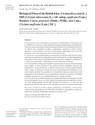
4.2 Ordination analysis of the vegetation and environmental data
A scatterplot of samples using Canonical Correspondence Analysis (CCA) shows a clear gradient
relating to the structural position of the samples on the shingle structure (Figure 4.1). The
predominant gradient is along axis 1 with seaward face samples occupying the top right corner of the
plot, ridge samples concentrated around the centre bottom, and backslope samples to the left of the
plot. A relationship is also evident, therefore, between the ridge samples (and to a lesser extent the
seaward face samples) and axis 2.
Figure 4.1. CCA scatterplot of Slapton samples, grouped according to structural position 1 =
seaward face, 2 = ridge, 3 = backslope
Axis 2
ST8
ST38
ST19
ST49
ST32
ST20
ST25
ST44
ST31
ST9
ST26
ST30
ST14
ST17
ST48
ST24
ST37
ST12
ST5
ST58
ST54
ST13
ST53
ST36
ST47
ST52
ST29
ST23
ST6
ST18
ST43
ST2
ST3
ST57
ST28
ST7
ST22
Axis 1
ST42
ST34
ST11
ST51
ST27
ST1
ST46
- 24 -
ST4
ST35
ST45
ST50
ST40
ST10
ST56
ST16
ST41
ST39
ST33
ST55
ST21
ST15
Strucpos
A Monte Carlo test (1000 runs) was applied to the analysis, testing the null hypothesis that there is no
relationship between the species and environmental variable matrices. Table 4.3 demonstrates a
positive relationship between matrices, particularly along axis 1 which accounts for a major
1
2
3

proportion of variation within the dataset. The first two axes have eigenvalues of 0.725 and 0.458
respectively (significance value for all axes p = 0.001).
Table 4.3. Monte Carlo test results from the CCA ordination of the Slapton data with the eigenvalues
shown for the first three axes
-------------------------------------------------------------------------
Randomized data
Real data Monte Carlo test, 999 runs
-------------------- ---------------------------------------------------
Axis Eigenvalue Mean Minimum Maximum p
-------------------------------------------------------------------------
1 0.725 0.344 0.226 0.533 0.0010
2 0.458 0.272 0.189 0.414 0.0010
3 0.386 0.222 0.151 0.343 0.0010
-------------------------------------------------------------------------
Similarly, a highly significant linear relationship exists between the species and environment data on
all three axes (Table 4.4). McCune & Mefford (1999) warn against assumptive interpretations of the
Pearson correlation in case of high values being the result of a high ratio between the number of
variables and samples. Although the significance of these results are demonstrated (p < 0.01 for axes
1 and 3, and p < 0.05 for axis 2), a measure of the strength of the species-environment relationship is
also seen in a Principal Components Analysis (PCA) (Table 4.5).
Table 4.4. Monte Carlo test results from the CCA ordination of the Slapton data with the speciesenvironment
Pearson correlation shown for the first three axes
---------------------------------------------------------------------------
Randomized data
Real data Monte Carlo test, 999 runs
------------ ---------------------------
Axis Spp-EnvtCorr. Mean Minimum Maximum p
---------------------------------------------------------------------------
1 0.918 0.764 0.656 0.885 0.0010
2 0.810 0.724 0.590 0.849 0.0120
3 0.803 0.691 0.563 0.815 0.0040
---------------------------------------------------------------------------
- 25 -

Table 4.5. Principal Components Analysis of the environmental dataset showing % variation
explained by the first 10 axes corresponding to environmental variables
----------------------------------------------------------------
Broken-stick
AXIS Eigenvalue % of Variance Cum. % of Var. Eigenvalue
----------------------------------------------------------------
1 4.177 37.975 37.975 3.020
2 2.251 20.465 58.441 2.020
3 1.313 11.940 70.381 1.520
4 0.898 8.164 78.545 1.187
5 0.874 7.947 86.491 0.937
6 0.485 4.409 90.901 0.737
7 0.344 3.131 94.031 0.570
8 0.245 2.229 96.260 0.427
9 0.161 1.461 97.722 0.302
10 0.140 1.269 98.991 0.191
-----------------------------------------------------------------
The three categories seen in Figure 4.1, reflecting the structural position of samples on the survey site,
can be considered natural vegetation groups following a zonal geomorphological pattern from
seashore to the edge of the leys. This general grouping has already been evidenced from the
TWINSPAN table 4.1. However, TWINSPAN generated eight assemblage groups that reflect
localized variation in vegetation within the broader structural zones. A complementary analysis
plotting these assemblage groups on the CCA ordination diagram show how the groups relate to each
other, and to the first two axes (Figure 4.2).
While there is a degree of overlap between several of the groups, reflecting reality in the field, clear
patterns emerge that show the variation amongst assemblages situated within the structural zones.
Groups 3, 4, 6 and 7 demonstrate the most obvious clustering while groups 1 and 2 have the most
internal variation. The latter two were subject to further division using TWINSPAN but did not result
in any more of a satisfactory outcome. Group 5 has a clear core of samples with a small number of
quadrats showing affinities to other groups. Group 8 is a single sample group.
When comparing Figures 4.1 and 4.2, it is evident that assemblage groups 1, 2 and 3 are varieties of
the backslope vegetation, occupying the left-hand side of the ordination plots. Group 4 is a small
transitional assemblage in the centre-left of the diagram. Groups 5, 7 and 8 reflect characteristics of
the ridge, although divided to centre-lower right, lower centre and bottom right hand corner of the plot
respectively. Group 6 represents the seaward face community dominating the upper right corner of the
ordination.
- 26 -

Figure 4.2. Complementary analysis of Slapton data showing the TWINSPAN derived vegetation
assemblage groups superimposed on the CCA ordination plot
Axis 2
ST8
ST38
ST19
ST49
ST32
ST20
ST25
ST31
ST44
ST30
ST9
ST14
ST17
ST26
ST48
ST24
ST37
ST12
ST58
ST13
ST5ST36
ST54
ST47
ST52
ST53
ST29
ST23
ST6
ST43
ST2
ST18
ST7
ST3
ST57
ST28
ST22
Axis 1
ST42
ST34
ST11
ST51
ST27
ST1
ST46
- 27 -
ST4
ST35
ST45
ST50
ST40
ST10
ST56
ST16
ST41
ST39
ST33
ST55
ST21
ST15
AssemGrp
In addition to species assemblages, a species ordination plot allows the position of each species to be
considered individually in relation to the axes and environmental gradients (Figure 4.3). The species
seen on the left/top left side of the ordination tend to be associated with the backslope vegetation,
such as Rubus fruticosus (Rubufrut on figure 4.3), those at the centre to lower right corner are more
likely to be found on the ridge i.e. Armeria maritima (Armemari) and the seaward face is represented
by species occupying the centre – top right of the plot, for example, Crithmum maritimum (Critmari).
Some species found near the centre of the diagram will be less specific, occurring equally on both the
backslope and ridge i.e. Festuca rubra and Digitalis purpurea.
1
2
3
4
5
6
7
8

Figure 4.3. CCA species ordination of Slapton data. See Appendix 3 for a full species list.
Axis 2
Chaetemu
Acerpseu
Prunspin
Fumaoffi
Betooffi
Rumeobtu
Rubufrut
Galiveru
Holcmoll
Galisaxa
Dauccaro
Trifrepe
Senejaco Senevulg
Lathprat
Gerarobe
Lolipere
Plancoro
Planmajo
Myosramo
Calysold
Glauflav
- 28 -
Armemari
Critmari
Euphpara
Crammari
Foenvulg
Anthoder
Bareshin
Teucscor Hedeheli Galimoll
Glechede
Urtidioi
Ulexspec
Vicisati
Cirspalu
Calysylv Arctminu
Phraaust
Poaannua
Betavulg
Siledioi
Galiapar
Dactglom Hyporadi
Elymfarc
Festarun
Heraspon Geramoll
Arrhelat
Festrubr
Centnigr
Centrube
Artevulg Trifdubi
Vulpbrom
Raphmari
Pilooffi Rumeacet Achimill
Taraoffi
Inulcrit
Digipurp Cochdani
Leonhisp
Anagarve
Poterept
Astelino Silemari
Cardtenu Vicihirs Soncoler
Rumecris
Echivulg Trifprat
Agrostol
Crepvesi
Centscab
Cerastsp
Ononrepe Cichinty
Pteraqui
Artearve
Bracpinn
Medihybr
Lotucorn
Planlanc Desmmari
Elymrepe Tripmari
Cirsarve
Bromarve
Holclana
Axis 1
Some of the environmental variables show quite high correlations with each other (Table 4.6). Soil
moisture content, soil pH and soil organic matter content are strongly correlated with one another, as
are shingle size and fine fraction. High intercorrelation can de-stabilize the canonical coefficients and
distort the outputs of the analysis affecting interpretation (Kent & Coker, 1992). Using a quadrat-
environment biplot from CCA, the correlation matrix and the results of a PCA, it was found that
removal of selected variables had a minimal impact on the orientation, eigenvalues, variance or
Trifcamp
Agrocapi
significance levels of the original ordination. If anything, removal slightly threatened ease of
interpretation. For example, when the pairing of shingle size and fine fraction was removed from the
data, the resultant ordination plot showed increased overlapping between the assemblage groups. It is
surprising, therefore, that these two variables account for just two and a half percent of the floristic
Trifsubt

variation. All variables were subsequently reinstated for the final ordination. The entire environmental
dataset can be seen in Appendix 4.
Table 4.6. The Pearson product-moment correlation matrix for the Slapton data environmental
variables
Slope Soilph Soildept Soiltemp Soilmois Soilorg Shinsize Finefrac
Slope 1.000 0.052 -0.050 0.040 0.050 -0.152 0.246 0.246
Soilph 0.052 1.000 -0.183 0.575 -0.671 -0.739 -0.083 0.154
Soildept -0.050 -0.183 1.000 -0.266 -0.062 0.140 -0.033 -0.181
Soiltemp 0.040 0.575 -0.266 1.000 -0.480 -0.530 -0.060 0.078
Soilmois 0.050 -0.671 -0.062 -0.480 1.000 0.682 0.227 0.150
Soilorg -0.152 -0.739 0.140 -0.530 0.682 1.000 -0.188 -0.267
Shinsize 0.246 -0.083 -0.033 -0.060 0.227 -0.188 1.000 0.758
Finefrac 0.246 0.154 -0.181 0.078 0.150 -0.267 0.758 1.000
A number of the environmental variables were important in structuring the CCA ordination (Table
4.7). Soil temperature, pH and organic matter content correspond to variation expressed along axis 1
with soil moisture also having some significance. Soil depth, shingle particle size and % fine fraction
are the most influential variables on axis 2, while only shingle size shows correlation with the third
axis. A number of gradients therefore appear to be present, particularly following axes 1 and 2.
Table 4.7. Intra-set correlations between environmental variables and ordination axes for the Slapton
data
--------------------------------------------------------------------
Correlations* Biplot Scores
Variable Axis 1 Axis 2 Axis 3 Axis 1 Axis 2 Axis 3
--------------------------------------------------------------------
1 Slope 0.085 0.187 0.286 0.073 0.127 0.177
2 Soilph 0.766 -0.017 0.153 0.652 -0.012 0.095
3 Soildept -0.205 0.646 0.247 -0.175 0.438 0.153
4 Soiltemp 0.815 -0.283 -0.277 0.694 -0.192 -0.172
5 Soilmois -0.595 -0.002 0.215 -0.507 -0.001 0.133
6 Soilorg -0.735 0.267 -0.281 -0.626 0.181 -0.174
7 Shinsize -0.122 -0.573 0.743 -0.104 -0.388 0.462
8 Finefrac -0.089 -0.553 0.435 -0.076 -0.374 0.270
------------------------------------------------------------------
These gradients can be seen more clearly when the environmental variables are graphically
represented on biplots. Figures 4.4 and 4.5 show the most important variables on a sample ordination
plot, and by superimposing the assemblage groups on one plot and the structural position zones on the
other, the relationships between environmental variables, samples, plant assemblages and physical
structure can be observed.
- 29 -

Figure 4.4. CCA sample biplot of axes 1 and 2 with samples reflecting their relative positions on the
physical shingle structure. 1 = seaward face, 2 = ridge, 3 = backslope.
Axis 2
ST8
ST38
ST19
ST49
ST32
ST20
ST25
ST44
ST9
ST31
ST30
ST14
Soilorg
ST17
ST26
ST48
ST24
ST37
ST13
ST12
ST58
Soilmois
ST5
ST36
ST54
ST47
ST52
ST53
ST29
Soildept
ST23
ST6
ST43
ST2
ST18 ST7
ST3
Shinsize Finefrac
ST57
ST28
ST22
Axis 1
ST42
ST34
ST11
ST51
ST1
Soilph
Soiltemp
ST4
ST35
ST27
ST46
ST45
ST50
ST40
- 30 -
ST10
ST56
ST16
ST41
ST39
ST33
ST55
ST21
ST15
Strucpos
Figure 4.5. CCA sample biplot of axes 1 and 2 with samples reflecting their relative positions within
the TWINSPAN derived plant assemblages
Axis 2
ST8
ST38
ST19
ST49
ST32
ST20
ST25
ST44
ST31
ST9
ST14
Soilorg
Soilmois
ST30
ST17
ST26
ST48
ST24
ST37
Soildept
ST12
ST58
ST13
ST5ST36
ST54
ST47
ST52
ST53
Shinsize
ST29
ST23
ST6
ST43
ST2
ST7
ST18
ST3
Finefrac
ST57
ST28
ST22
Axis 1
ST34
ST11
ST42
ST1
Soilph
ST51
Soiltemp
ST27
ST46
ST4
ST35
ST45
ST50
ST40
ST10
ST56
ST16
ST41
ST39
ST33
ST55
ST21
ST15
1
2
3
AssemGrp
1
2
3
4
5
6
7
8

The biplots show that no single variable is particularly dominant with its influence on variation
overall. This is reflected by the similar lengths of the arrows. The plot does show, however, which
variables are particularly important for the distribution of the plant assemblages i.e. soil pH and soil
temperature for groups 5 and 6, soil organic matter to group 2 etc. The position of the arrows in
relation to the axes indicates how closely the axes are correlated to that variable. The correlations
given in Table 4.7 are clearly supported by the biplots, with the gradients very evident.
Figures 4.6 and 4.7 give a clearer understanding of the major environmental gradients that influence
the patterns in species composition. The side scatterplots reveal the extent of change along the
gradients even when this is not at first obvious on the main plot. This information can be used by
managers to influence certain decisions that need to be made in respect of habitat or species
management. For example, the aim of increasing the proportion of the shingle bar with herb-rich
Festuca grassland is enhanced by the knowledge that this community responds to higher temperature,
neutral to higher pH substrata with low moisture and organic matter content. This type of community
is more likely to succeed over time, therefore, if shingle is spread over the ridge rather than importing
finer soils. However, the short-term implications may be a patchier surface which is less aesthetically
pleasing. With the knowledge though, more informed choices can be made.
As well as analyzing data with a view to identifying gradients across the shingle structure, the
possibility of a gradient along the structure (parallel to the shore and road from Strete Gate to
Torcross) was also investigated. The environmental data was condensed into ‘whole transect samples’
using mean values from each suite of quadrats making up the transects. This gave one value for each
environmental variable for each transect. Figure 4.8 shows that most of the variables have peaks and
troughs but no overall discernable trend. Soil pH, shingle size, slope and soil temperature display little
variation between the transects. The two exceptions are soil depth which decreases overall toward the
Torcross end of the site, and % fine fraction which increases in the same direction, both of which can
probably be explained by the higher frequencies of trampling observed around the southern end of the
site. Of the 217,521 visitors to the ridge in 2003, 52% used the car parks at Torcross as their base for
the visit (SLNNR, 2005), with many walking along part of the ridge or backslope toward the central
memorial car park and back.
- 31 -

Figure 4.6. CCA ordination of selected variables with gradients along axis 1. The size of the circles
indicates the magnitude of the values. Axis 1 profiles are shown below each variable to demonstrate
the rate of change along the gradient.
Axis 2
28
24
20
16
12
pH Soil organic matter content
Axis 1
Axis 2
10
8
6
4
Soil temperature
Axis 1
- 32 -
Axis 2
60
40
20
0
Axis 1

Figure 4.7. CCA ordination of selected variables with gradients along axis 2. The size of the circles
indicates the magnitude of the values. Axis 2 profiles are shown aside each variable to demonstrate
the rate of change along the gradient.
Soil depth
0 20 40 60 80
Fine fraction
0 20 40 60 80
Axis 2
Axis 2
Axis 1
Axis 1
- 33 -

Figure 4.8. Profiles of environmental variable gradients from Strete Gate (T1) to Torcross
(T11)
80.000
70.000
60.000
50.000
Mean value
40.000
30.000
20.000
10.000
0.000
T1 T2 T3 T4 T5 T6 T7 T8 T9 T10 T11
Transect no.
4.3 Patterns of floristic diversity on the shingle bar
A statistical summary of the sample data from PC ORD (McClune & Mefford, 1999) reveals that the
mean species richness for the whole survey site is 10 species per sample, and mean Shannon diversity
index is 1.37. Much of the floristic diversity is explained by the high occurrence of rare species with a
mean cover value of just 1.483%. There is no continuous trend in species richness or diversity as one
moves from Strete Gate to Torcross, but Figure 4.9 (a) does show higher values for transects 7-10
which situate opposite the lower ley. Samples positioned on the ridge have the highest mean richness
and diversity (b), and if the one-sample group 8 is excluded, assemblage groups 3, 4 and 5 are the
most diverse and species rich (c). Quadrat ST46 has the highest species richness (20). This sample is
located on the ridge; in transect 9, within assemblage group 5. The highest diversity index (2.402) is
found in quadrat ST41, also situated on the ridge; in transect 8, also within assemblage group 5.
- 34 -
Slope
Soilph
Soildept
Soiltemp
Soilmois
Soilorg
Shinsize
Finefract

Figure 4.9. Statistical summary of species richness and Shannon diversity indices for the vegetation
data of Slapton. (a) Mean values for each transect, (b) Mean values for each structural position, (c)
Mean values for each TWINSPAN assemblage group (Table 4.1).
a
b
c
Mean value
Mean value
Mean value
16
14
12
10
8
6
4
2
0
14
12
10
8
6
4
2
0
16
14
12
10
8
6
4
2
0
1 2 3 4 5 6 7 8 9 10 11
Transect number
Seaward face Ridge Backslope
Structural position
1 2 3 4 5 6 7 8
Assemblage group number
- 35 -
Mean S
Mean H
Mean S
Mean H
Mean S
Mean H

5. DISCUSSION AND CONCLUSIONS
5.1 Two-way indicator species analysis and ordination to provide definitions of
plant assemblages
The TWINSPAN analysis (Table 4.1) reveals some general divisions between habitat types. Scrub
and coarse mixed grassland assemblages occur at the upper part of the table, and are typical of the
backslope ecology. Herb-rich grassland of the shingle ridge is found in the centre-lower part of the
table, and those assemblages more representative of exposed seaward face pioneer vegetation are
located at the bottom of the table.
The distribution of the samples on the CCA ordination (Figure 4.1) is a good reflection of the general
grouping by structural position with a clear pattern visible. The obvious outlier in the seaward face
community (group 1) is ST27, this quadrat being located on a two metre strip of disturbed ruderal
shingle vegetation running along the edge of the monument car park. The shingle was particularly
shallow here, situated over a now-buried concrete defence wall. Fresh shingle had been bulldozed up
from the lower shore just a few days before sampling, possibly covering some vegetation stands.
Although a number of the species are typical pioneers, the presence of Elymus repens at its highest
abundance is probably the most divisive factor, marginalising the sample from the remainder of the
group.
The ridge community shows relatively high variation with three potential sample clusters. Two of
these relate closely to the TWINSPAN assemblages. Samples ST11, 35, 40, 41, 46, 51 and 56 fall
within assemblage group 5, while ST22, 23, 28, 29 and 34 represent assemblage group 7. ST16 stands
alone, with the remaining samples placed into differing groups. The reason for these displacements is
most likely due to the environmental data i.e. ST5 and 6 have a lower soil temperature or greater
depth than the majority of the ridge samples (Figures 4.5, 4.6 and 4.7).
The samples from the backslope also display internal variation, mostly in relation to axis 2, reflecting
changes in soil depth and, to a lesser extent, shingle size and % fine fraction (Table 4.7). Quadrats
ST8, 9, 14, 19, 20, 31, 37, and 38 could be considered separate to the core of the group creating a
diagonal division along a soil organic content gradient (Figure 4.4). This could reflect a further
assemblage or a sub-group highlighted by the ordination but not picked up by the classification
- 36 -

process. ST42 is the backslope sample furthest to the right of the plot, close to the core of the ridge
samples, with environmental data more akin to these samples i.e. higher pH than most backslope
samples (8.15), low soil moisture and soil organic content. A mat of Festuca rubra with species such
as Rumex crispus, Achillea millefolium and Echium vulgare contributed to the sample’s similarity to
those of the ridge. This potential sub-community resembles Sneddon & Randall’s (1994) SH65
Festuca rubra-Achillea millefolium-Lotus corniculatus community.
More precise and detailed classification groups derived from the TWINSPAN analysis are shown in
Table 4.2. Eight assemblage groups were defined, although group 8 is a single sample group. An
attempt has been made to compare each group with the closest matching NVC categories using
Rodwell (1991, 1992, 2000). One of the original aims of this research was to produce an NVC
vegetation map of the Slapton shingle bar for use by the Nature Reserve managers. The map was to be
based on the matching of classified groups with NVC communities using MAVIS software. The
project aims have subsequently been re-prioritised to ensure compliance with time restrictions and
focus on community analysis, although a brief attempt has been made manually to identify similar
NVC communities as well as those defined by Sneddon & Randall (1994).
Rather than ignore outliers and within-group variation, an attempt has been made to describe and
explain such occurrences.
Assemblage Group 1 - Rubus fruticosus – Hedera helix – Raphanus maritimus scrub community
Assemblage one consists of six samples characterised by high constancies of Rubus fruticosus,
Hedera helix and Raphanus maritimus, and the associates Heracleum sphondylium, Prunus spinosa
and Ulex species. Hedera is most often present as an extensive ground carpet around and beneath the
scrub. This group most approximates to the NVC category W22 Prunus spinosa – Rubus fruticosus
scrub, but with a local maritime influence.
The Rubus fruticosus – Hedera helix – Raphanus maritimus scrub community is a feature of the
backslope and its position on the left side of the ordination plot reflects the preference for lower
temperature base-poor soils high in moisture and organic matter content (Figures 4.2, 4.5). Of the two
samples within this group but lower down the second axis, ST32 has the most acidic soil of the entire
site. A pH of 4.23 falls within an optimum range of Pteridium aquilinum (Rodwell, 1991), occurring
rarely but in abundance. The significant presence of Rubus fruticosus in the same sample points to a
- 37 -

small Pteridium aquilinum – Rubus fruticosus underscrub (NVC category W25) occurring near the
shore of the ley, at the northern end of the Lower Ley. Sneddon & Randall (1994) identified this
similarly as a Pteridium aquilinum-Arrhenatherum elatius-Rubus fruticosus community with the
dominance of Pteridium excluding many other associates.
ST17 is unique in that it is a ridge sample situated adjacent to the well-trampled surface of the former
coastal road which was re-routed 20m inland in 2001. Prior to the road realignment, it is likely that
this patch of vegetation lay alongside the coastal footpath that runs along the length of the backslope.
In effect, the road has ‘leapfrogged’ a strip of backslope vegetation and the path that passed through
the middle of this vegetation (Figure 4.1). The semi-compacted surface explains the lower soil depth
that defines the position of the sample lower down the second axis on the CCA plot (Figure 4.2). The
soil also has the lowest pH of all ridge samples (6.44) explaining the separation of this sample from its
geographical counterparts along axis 1. Rubus fruticosus and Ulex species both feature prominently
within this sample, reflecting its former status as part of the backslope community. Although ST17
has been placed within assemblage group one as part of the TWINSPAN analysis, it does have
features in common with the Arrhenatherum elatius – Rubus fruticosus community of assemblage
two. However, from field observations it is likely that the sampling strategy has under- represented a
notable change from the scrub described in this assemblage to a distinct Ulex – Rubus fruticosus scrub
community. This change occurs over a south – north gradient and ST17 would have been part of this
community prior to the road re-alignment.).
Figure 5.1 Section of the A379 just north of Slapton Bridge. A. After storm damage but prior to road
re-alignment. Large boulders were placed on the seaward face to protect the development. The lighter
backslope pathway can be seen running through the darker scrub close to the road. B. The road re-
aligned through the backslope scrub, creating an ‘artificial’ ridge formed from the former road,
backslope pathway, and backslope vegetation. The approximate line of transect 4, which includes
quadrat ST17, has been superimposed.
A B
- 38 -

Assemblage Group 2 – Arrhenatherum elatius grassland – Rubus fruticosus scrub community
This larger assemblage of thirteen samples is characterised by the constant presence of
Arrhenatherum elatius, Raphanus maritimus, Heracleum sphondylium, Rubus fruticosus and Urtica
dioica, while Dactylis glomerata, Galium aparine and Hedera helix are occasional associates.
Mixtures of these species may occur as a sub-community of assemblage 1 or form patches throughout
the scrub. This assemblage corresponds largely to NVC category MG1b, Arrhenatheretum, Urtica
dioica sub-community, although often forming a local mosaic with Rubus fruticosus stands, and with
the constant addition of Raphanus maritimus.
The assemblage appears, in its entirety, over to the left side of the ordination (Figure 4.2)
corresponding to lower soil temperatures, lower pH, high soil moisture and soil organic matter
content. It is therefore not surprising that this scrub community is almost entirely situated on the
backslope.Variation within the group separates samples ST8, 14, 31, 37, 38 and 44 from the rest of
the group on axis 2, although the TWINSPAN analysis does not encourage the formation of a discreet
assemblage. This internal variation follows a % fine fraction gradient, Figure 4.7 showing the lower
values for the above samples positioned toward the top left corner of the plot. The changes in soil
organic matter content also represent a significant gradient dividing this group up (Figure 4.6). The
main impact of these changes on species composition appears to centre on the low presence or
absence of scrub species among the lower – central samples, possibly representing a transition toward
assemblage group 3.
- 39 -

Assemblage Group 3 – Arrhenatherum elatius – Raphanus maritimus community
The nine samples of this group comprise of Raphanus maritimus, Dactylis glomerata, Festuca rubra,
Arrhenatherum elatius, Heracleum sphondylium and Rubus fruticosus as the constants. Hedera helix,
Vicia sativa and Achillea millefolium are common associates, while Artemisia vulgaris, Galium
mollugo and Rumex crispus are occasional. This mixed- grassland group resembles NVC class MG1a,
an Arrhenatheretum, Festuca rubra sub-community. Again, the continual presence of Raphanus
maritimus suggests a local unique sub-community. Figure 5.2 gives an example of how this
community looks on much of the backslope.
Figure 5.2. Rough grassland showing the dominance of Arrhenatherum elatius and Raphanus
maritimus. Also visible are Dactylis glomerata, Heracleum sphondylium and Digitalis purpurea.
The complementary analysis (Figure 4.2) shows that while this well-clustered assemblage is also
responsive to low pH values, it occupies a slightly more central position on the plot as a consequence
of much lower soil organic matter content, increasing soil temperatures and a high percentage of fine
fraction. This is the most dominant community of the backslope, which has expanded over the years
replacing more diverse mixed grassland of Anthoxanthum, Agrostis, Festuca rubra and Holcus
- 40 -

lanatus, as recorded by Brookes & Burns (1969). During the course of data collection for this work,
local residents and regular visitors bemoaned the perceived rapid increase in the occurrence of
Raphanus maritimus at the expense of more visually pleasing herb varieties. Table 5.1 provides an
indication of the sustained dispersal of Raphanus onto the ridge during the last ten years.
Assemblage Group 4 – Festuca rubra – Achillea millefolium grassland community
Assemblage 4 is dominated by Festuca rubra, Achillea millefolium and Heracleum sphondylium.
Because there are just three samples in this group, there are a number of minor constants. These are: -
Arrhenatherum elatius, Rubus fruticosus, Rumex acetosa, Lathyris pratensis, Potentilla reptans,
Centaurea nigra, Lotus corniculatis, Plantago lanceolata, and Ononis repens. There is no adequate
NVC group resembling the above assemblage, although the SD8a Festuca rubra – Galium verum
typical sub-community has been cited as being best matched to such groupings (Sneddon & Randall,
1993).
This small group forms a near-vertical linear relationship near the centre of the ordination,
characterized by neutral soils and fairly low soil temperatures, with the position in relation to axis 1
balanced by two low soil moisture values and one much higher. The most significant inter-sample
variation in species composition is the inclusion of Rubus fruticosus (40% cover) in ST7. This is a
transitional community in which a number of the species are found equally on the ridge and
backslope.
Assemblage Group 5 – Maritime herb grassland community
This assemblage includes ten samples but is no less diverse than the previous group. It is a more open,
patchy community with bare shingle accounting for over 20% cover in over half of the samples. The
community is relatively immature and there are no dominant species, the major elements being
Plantago lanceolata, Ononis repens, Achillea millefolium, Tripleurospermum maritimum,
Desmazaria marina, and Festuca rubra, while the common associates are Raphanus maritimus,
Armeria maritima, Silene maritima, Trifolium repens, and Lotus corniculatis. Once again, there is no
obvious satisfactory equivalent within the NVC structure. Sneddon & Randall (1993) describe the
same assemblage as a Festuca rubra – Achillea millefolium – Lotus corniculatis – Silene maritima
community which they assign to the NVC code SD7c (Ammophila arenaria – Festuca rubra semi-
fixed dune, Ononis repens sub-community).
- 41 -

Figure 4.2 shows this common ridge assemblage to have a positive relationship with axis 1 in relation
to soil temperature and a negative relationship with regard to soil moisture content. An increasing soil
pH also has a role to play in determining vegetation distribution. Sample ST34 appears on the
ordination plot closer to assemblage group 7. This may reflect the position of the quadrat near to one
of four permanent exclosure plots laid out along the top of the ridge between the central monument
car park and Torcross. Members of the public are forced to walk either side of the plot creating
informal ‘paths’ along the edges of the ridge. Half of ST34 was situated over one of these well
trodden paths and half over adjoining less-trampled vegetation. There are no obvious discrepancies
between this sample and the others of assemblage 5. The quantity of bare shingle may be a little
higher than most (30%) and % fine fraction is relatively high. The proximity of the samples to areas
of heavy trampling provides a link between this sample and those of assemblage 7, while revealing
the main difference between the two assemblages.
The species diversity of this community appears to have remained fairly stable over the past twenty
years (Table 4.1 but note subjective definitions) at 12/13 significant species. The constant elements
remain year on year, supporting the above definition of this assemblage group. It would be interesting
to maintain this comparison with future surveys, perhaps using the definitions given here to assist.
This could also provide a further tool to monitor progress of targets relating to management of the
shingle ridge grassland community, as per the SLNNR management plan.
With regard to the information contained in Table 5.1, some species will inevitably come and go over
the seasons, which may be dependent on the adopted sampling strategy. In the current case, for
example, species such as Daucus carota and Echium vulgare are almost certainly under-represented.
This table should be considered with caution and used as a general indicator or pointer for
clarification. A few species appear to have gone for good as a constant e.g. Leontodon spp., Crepis
vesicaria, Aira spp., while a number have appeared only once. The notable species’ to have made a
reappearance in 2005 are Tripleurospermum maritimum and Plantago coronopus, and new additions
to the major components list are Desmazeria marina, Trifolium repens and Lolium perenne. The latter
appears mostly as a result of the amenity community near to the car parks. Overall, the number of
major species has remained fairly constant (12-13) over the last four surveys.
- 42 -

Table 5.1. Species listed as major components of the ridge vegetation in five surveys (Brookes &
Burns, 1969; Cole, 1984; Sneddon & Randall, 1994; Wilson, 2002; this report, 2005). The definitions
of ‘major components’ from previous surveys are not known. For this survey, species are included if
they appear in assemblage 5 or assemblage 7 at ≥ 50% constancy
1969 1984 1994 2002 2005
Festuca rubra + + + + +
Silene maritima + + + +
Ononis repens + + + + +
Lotus corniculatus + + +
Leontodon spp + +
Hypochoeris radicata + + +
Crepis vesicaria +
Daucus carota + + +
Echium vulgare + +
Aira spp +
Tripleurospermum
+ +
inodorum ssp maritima
Armeria maritima + + + +
Achillea millefolium + + + +
Plantago lanceolata + + + +
Plantago coronopus + +
Galium verum +
Geranium molle +
Bellis perennis +
Trifolium dubium +
Poa pratensis +
Bromus hordaceus +
Heracleum sphondylium +
Taraxacum sp +
Raphanus raphanistrum ssp
+ +
maritimus
Desmazaria marina +
Trifolium repens +
Lolium perenne +
Assemblage Group 6 – Tripleurospermum maritimum – Glaucium flavum pioneer community
The eleven samples within this community form an open pioneer assemblage with all species present
offering low percentage cover within the samples. An average of 88% of cover per sample is bare
shingle. Tripleurospermum maritimum and Glaucium flavum are the only species to appear with any
degree of frequency, with a number of patchy associates present, including Beta vulgaris, Elymus
farctus ssp. boreali-atlanticus, Euphorbia paralias, Crithmum maritimum, Ononis repens and
- 43 -

Plantago coronopus. Figure 4.3 shows several of these species co-existing on a section of the seaward
face toward the southern end of the beach. The closest NVC match to this group appears to be the
SD1 Rumex crispus – Glaucium flavum shingle community, albeit with Rumex being replaced by
Tripleurospermum. Crambe maritima, a rare species of the SD1 community, appears in just one
sample here due mostly to its very patchy occurrence, although there are approximately 50-60
individual stands in total. The locally strong presence of Elymus farctus in limited 1-3m strips along
the seaward edge of the ridge, with Euphorbia paralias, may also point toward an SD4 Elymus farctus
ssp. Boreali-atlanticus foredune community.
Figures 4.2, 4.5, 4.6 and 4.7 demonstrate the positive correlations between this assemblage and both
axes. High soil pH, high soil temperatures and increased depth (which is perhaps to be expected on
open shingle), are the environmental variables measured that characterize this open community. Less
quantity of fine fraction (Figure 4.7) is another fairly obvious feature of the seaward face compared to
the more stable ridge and backslope.
Figure 5.3. Several strandline species exemplifying assemblage group 6, occurring together at a
section with no clear boundary between the edge of the seaward face and the ridge. Species present
include Elymus farctus ssp. boreali- atlanticus, Ononis repens, Crambe maritima, Tripleurospermum
maritimum, Euphorbia paralias and Plantago coronopus.
- 44 -

Assemblage Group 7 – Lolium perenne – Plantago lanceolata grassland
Assemblage 7 is a smaller group of five samples making up a community defined by the constant
presence of Trifolium repens, Lolium perenne, Plantago lanceolata and Plantago coronopus. In some
stands, Lolium perenne may have been partially replaced by Holcus lanatus, Dactylis glomerata or
Festuca rubra. The constant presence of Plantago species suggests the stands are older (Rodwell,
1992) with more open swards. This group corresponds to NVC category MG7e Lolium perenne –
Plantago lanceolata grassland sub-community.
This assemblage is well defined on the ordination, forming a loose cluster in the lower – central
region of the plot (Figure 4.2), corresponding negatively to a soil depth gradient and positively to a
fine fraction gradient (Figures 4.5, 3.7). All the samples from this community are from sites on the
ridge that are well trampled amenity locations or frequently used pathways i.e. around the war
memorial; on the former overflow car park adjacent to the existing memorial car park; and on the thin
strip of ruderal vegetation between the road and car park at Torcross. It is possible that a cultivar of
Lolium perenne has been used for some of these amenity swards because of its resistance to heavy use
(Rodwell, 1992).
Assemblage Group 8 – Agrostis capillaris – Trifolium species grassland
This group consists of just one sample with fifteen species. Those species with the highest % cover
are Trifolium campestre, Plantago coronopus, Agrostis capillaris and Trifolium repens.
The sample is clearly seen on the ordination situated in the lower right corner of the plot, its
environmental features including high pH (8.3), low organic matter content, high temperature and %
fine fraction, and the shallowest soil of all samples in the survey (Figures 4.2, 4.5, 4.6, 4.7).
A good match to the NVC categories is not straightforward and should be treated with extreme
caution from just one sample. There is a passing resemblance to the U4 Festuca ovina – Agrostis
capillaris – Galium saxatile grassland, Holcus lanatus – Trifolium repens sub-community. However,
there is also a possibility that the sample represents a younger version of assemblage group 7, bearing
in mind its position on the compacted, stony former road site which has been used as a convenient
- 45 -

footpath over the past four years. Many of the species present exemplify trampled surfaces, including
Poa annua, Trifolium repens, Plantago coronopus and Lolium perenne.
5.2 Environmental gradients
The results of this survey have shown that the environmental variables measured are significant in
explaining floristic variation (Tables 4.4, 4.5, 4.7; Figures 4.4 and 4.5). These variables have been
examined in relation to the structural position of the samples, and to the TWINSPAN defined
assemblage groups.
The possibility of environmental variation along the shingle structure was also explored with a view
to explaining any patchiness amongst the assemblages that may not be correlated with structural
position. Figure 4.8 demonstrates that soil depth follows a general pattern of decreasing values from
Strete Gate to Torcross, with a specific trough between transects 5 and 8. This trend is explained by a
number of factors. Larger sections of the soil are compacted by trampling due to greater numbers of
visitors walking between Torcross and the monument car park compared to the northern end of the
site (Slapton Ley National Nature Reserve, 2005). Some of the ridge samples are situated on the
former monument overflow car park, hence the surface soil is thin and stony, and one of the seaward
face quadrats was laid over the base of a sea defence wall buried just below the shingle surface. The
soils on the backslope also tended to be shallower in this section of the site. Although survey notes
record a change in the properties of the soil to a soft, light, red-brown soil lacking shingle content, no
explanation for the reduction in depth is offered here with any certainty. It is possible that the soil in
this area was imported as part of the road realignment works, or to cover the ground following
burning of scrub in an attempt at partial clearance.
The other notable trend is the increase in % fine fraction from Strete Gate to Torcross. The biggest
contribution to this gradient is found within transect 9, which contains particularly high diversity
samples. A possible link therefore exists between these two factors, with a greater chance of finer
sediment being trapped among the more abundant plant material.
- 46 -

Despite the above trends, it is difficult to see a causal relationship between variation in environmental
measurements and variation in plant assemblages along the shingle structure, and it is suggested that
any correlations in practice are purely local in nature.
5.3 Floristic diversity
Despite the claims of Chapman (1976) that shingle beaches are not floristically rich, an average
species richness of 10 species per sample and a maximum of 20 species in one sample, provide
justification for continued interest and conservation action in relation to this habitat.
The greatest plant species diversity is found between transects 7 and 10 (Figure 4.9a) between
Torcross and Slapton Bridge. From the species data, this increase in diversity corresponds to a
particularly species rich section of strandline pioneer vegetation, a wide variety of shrubs that appear
to be tolerant of trampling on the ridge, and minimal presence of scrub on the backslope.
Diversity is generally higher within the ridge communities than the backslope, reflecting the greater
impact of rough grassland invasion and scrub prominence on floristic variation than higher levels of
moisture and nutrients in the soil. Figures 4.9a and b, together with raw sample data and summary
statistics suggest that trampling need not be a barrier to plant diversity, with individual samples of the
highest diversity being situated on well-worn sections of the shingle ridge. The quadrat with the
highest number of species included a bare shingle patch covering 45% of the sample area. This
supports Mitchell & Kirby (1990) who concluded that light trampling by herbivores can increase plant
diversity.
The above trend is reinforced by three out of four of the highest diversity assemblage groups
associating mostly with the shingle ridge (Figure 4.9c). Group 3, the Arrhenatherum elatius –
Raphanus maritimus community, has one of the highest levels of species richness but lower diversity
than the ridge- based assemblages. This reflects the dominance of the two named species on the
backslope communities. The fact that the backslope shows lower plant diversity than the ridge, yet
assemblage 3 is relatively species rich, strongly suggests a negative effect on diversity of the scrub
communities commonly occurring on the central and northern sections of the backslope.
- 47 -

Because of its vulnerability to natural forces and human impacts, and the rarity of some of its
characteristic species, it is not surprising that the pioneer assemblage group 6 has the lowest species
richness and diversity. However, the baseline mean values for these indices can be used by managers
to measure progress on targets for increasing the stability of the strandline community over time.
Changes in species richness are not just a matter of increasing soil moisture, organic matter and fine
fraction to enhance nutrient levels. Otherwise there would be a straightforward trend of increasing
diversity from beach to lake. Figure 4.9b demonstrates that this is not the case – the ridge is most
diverse. Factors such as trampling intensity, management regimes, proximity to salt spray, and
lacustrine influences could all potentially affect plant diversity and spatial distribution in this location.
It may prove worthwhile for the Reserve managers to have such information quantified as part of
further research.
The research material on floristic diversity can be related to English Nature’s concern about diversity
levels on the backslope and associated non-favourable SSSI status of the structure. The information
can be used purely for monitoring purposes, or for influencing decisions on competing priorities
(Table 1.1 and management plan objectives).
5.4 Floristic patterns relating to the structure of the shingle bar
As well as the patterns previously described within the plant assemblages, there are also differences
between assemblages at the landscape scale. The most notable variation in pattern once again follows
the changes in structural zones. The pioneer community is very noticeably sparse and only occurs as a
distinct assemblage in two sections of the seaward face, one to the north end of the beach and one
between Torcross and the central car park. For the remainder of the site, the community is limited to a
thin strip of vegetation among bare shingle.
The vegetation on the ridge is mostly patchy, with a mosaic of Festuca grassland and maritime herbs
growing around bare patches of shingle. Although some large shingle patches encroach the ridge to
the north of the structure, the southern end of the bar is patchier, with the increased levels of
recreational use.
- 48 -

The backslope communities represent more of a continuum but a distinct scrub-grassland mosaic is
recognisable along much of the length of the bar. Generally, grassland dominates the southern end of
the backslope while scrub dominates the north.
The methodology using interrupted transects helped to identify mini-ecotones. The most obvious of
these were the strips of vegetation observed along the boundaries between ridge and road, road and
backslope, homogenous backslope community and pathway, and between backslope and ley. These
were not generally sampled because they only tended to be 0.5-1.0m wide and did not support the
aims and methods of the survey. It is acknowledged that these boundaries run along the length of the
shingle bar, therefore the assemblages associated with them could be considered discreet ecotone
communities and, as van der Maarel (1990) claims generally, should perhaps be afforded more
attention in future research.
5.5 Research limitations
It is likely that some scrub species were under sampled i.e. Ulex. This means that the variation within
scrub communities may not be fully reflected in the assemblage groupings. Because scrub stands are
very patchy, the sampling strategy used here is more likely to miss the patches than hit them, even
though they may be common. The same applies to some of the pioneer species such as Crambe
maritime which occur as large stands spaced far apart. A varied sampling strategy could be used for
future research to minimise this.
Ordination of species data and environmental data will not match precisely because species
distribution will be determined by factors other than environmental ones i.e. competition and plant
species strategies, as well as other abiotic factors not measured here.
The matter of temporal patchiness (Bullock, 1996) is often overlooked where plant abundance and
cover change over the seasons. Due to sampling being undertaken in summer, winter annuals and
vernal perennials may have been missed on occasion.
Species variation within some groups, such as brambles and gorse, was not always identified and will
therefore not be reflected in the results.
- 49 -

For the data collection, access to some of the more dense stands were difficult or not possible, hence
floristic data were estimated and abiotic data taken from the nearest accessible position in such
circumstances.
In any numerical classification system, the selection of groups is subjective, based on the ecological
knowledge of author. It is acknowledged that more experienced ecologists may have presented the
plant assemblages differently.
5.6 How does this research contribute to the objectives of the SLNNR
management plan?
The knowledge obtained from the analyses of the community and environmental data, as well as
information gained from the literature and site observations, can be usefully applied to the key issues
facing the managers of the Slapton Ley nature reserve. This is presented as a series of comments and
recommendations:
o The plan refers to the vegetated communities but does not state how they are to be
defined. The definitions given in this report could be useful here.
o One of the proposals involves the mechanical removal of turf to allow diverse growth
over time. This has been done previously at Slapton to control scrub, but led to the
formation of a ruderal flora rather than reverting to a grassland flora (Sneddon &
Randall, 1994)
o It could be difficult to re-introduce grazing without affecting the scrub, which is
subject to a planned increase in volume. Grazing could reduce most of the shrubs
(Chapman, 1976). There are cases where grazing has been found to increase plant
diversity (Putman et al., 1991) but this would be reversed if the species left behind
make up a species poor community (Grant et al., 1987). More detailed research into the
likely effects of grazing should be conducted prior to introduction
- 50 -

o There seems to be no account for the impact on some of the targets from storm
damage. For example, the target of increasing the proportion of pioneer strandline
vegetation in relation to the whole structure could be met year on year until a major
storm strikes. This places immense pressure on managers for something which is
beyond their control. Targets focused on increasing the opportunity for community
expansion would be more realistic and sustainable
o To maintain the Festuca ridge grassland, as per a further objective, it is suggested that
the ridge is not permitted to be encroached by scrub i.e. patches near Strete Gate and
on the site of road re-alignment. The levels of trampling should be better managed by
implementing a pedestrian scheme preferably along the length of the ridge, or at least
prioritized around each of the three car parks. Light trampling can actually increase
species diversity i.e. by opening swards up for new species, (as evidenced here) but
heavy trampling can destroy vegetation cover (Mitchell et al., 1990) (as suspected on
the southern end of the ridge)
o To increase pioneer vegetated shingle, immediately put a halt to vehicular access along
the beach so close to the ridge. Positive conditions include high soil temp, high pH,
deep soil, low moisture and organic content, which should therefore be considered as
part of any management decisions i.e. transplanting beach material
o There are some patches of the Lolium perenne-Plantago lanceolata community. If
mowing of these is reduced i.e. to just once a year, and mechanisms implemented to
reduce trampling, this is likely to encourage invasion by Arrhenatherum elatius
(Rodwell, 1992). Hence, managers need to be aware that fulfilling one objective
(reduction of erosion from trampling) may impact on other objectives (discouraging
growth of mature grasses)
o A possible conflict arises between targets for reducing coarse grassland and increasing
scrub, if one accepts that the former succeeds to the latter. This is another area that
would benefit more attention.
- 51 -

o It is not clear what the rationale is for increasing the amount of scrub, but it is
suspected to be associated with the presence of Cetti Warbler’s (Cettia cetti), dormice
(Muscardinus avellanarius) and/or scarce lichens. There is potential further conflict
between encouraging these communities and increasing plant diversity along the
backslope. This needs care with planning if a balance is to be struck between these
objectives.
o Allowing the proportion of scrub on the backslope to increase may threaten the
likelihood of increasing plant diversity. The fall in backslope species diversity over
time is a concern for English Nature and has contributed to the Reserve’s unfavourable
SSSI status.
o A number of pioneer species are associated with the drift-laden portion of the beach
i.e. Elymus farctus, Glaucium flavum, Rumex crispus, and Silene maritime (Chapman,
1976). Therefore, if managers wish to expand this community as per the management
plan, then the actions of the local council in regularly removing the drift material from
the beach should be halted. This has aesthetic consequences but it is possible to pilot
this in certain locations, with explanations and education offered to the public
Further recommendations relating to the research aspect of this project would include the production
of a vegetation map identifying plant communities in the field. This could use the categories of the
NVC or Sneddon & Randall (1994). If the NVC system is to be used, MAVIS, TABLEFIT or similar
software can match the categories to the observed communities. Aerial photographs of the site are
available from English Nature and provide a further tool for a mapping exercise.
5.7 Conclusions
1. The nature of the plant communities at Slapton has been described by reference to species
assemblages. A phytosociological classification was produced and the relationships between
species composition and a range of environmental variables were examined using multivariate
techniques.
- 52 -

2. The results generally match expectations and previous surveys, although a number of
differences within species assemblage compositions exist. The single-community ridge
vegetation defined by Wilson (2002) has been separated into three sub-communities, based on
groupings produced by a TWINSPAN analysis.
3. The classification shows vegetation at Slapton is not wholly typical of shingle formations.
Although there is a danger in making assumptions about temporal change from just one
survey, the patterns of the plant communities do not obviously match the succession model of
Randall & Sneddon (2001). This area of work would be worthy of further research to identify
how, and why, the species composition at Slapton varies from the ‘typical’ shingle
community.
4. The relationships between species composition and environmental variables are not entirely
unexpected although the importance of shingle size was not realised.
5. The distribution of the plant communities is mainly determined by the interaction of soil pH,
soil temperature, soil moisture and organic matter content. Soil depth and % of fine fraction
also have an impact on species composition. Recreational use and management are important,
although the difficulty of identifying objective measures of these pressures within a short time
frame is a major problem, and would be a useful subject for more detailed investigation.
6. The shingle ridge vegetation does not consist of one homogeneous community, but shows
variation relating largely to local intensities of recreational use. The floristic diversity is higher
on the ridge compared to the grassland-scrub communities of the backslope.
7. A series of comments and recommendations have been presented in response to the Slapton
Ley National Nature Reserve management plan, which should contribute to the monitoring
and evaluation of specific objectives relating to the status of the shingle ridge.
- 53 -

Appendix 1: Example of a completed front page of an NVC-based record sheet and
species list
- 54 -

Appendix 2: Particle Grade-Size Scale
- 55 -

Appendix 3. Species list
Cochdani Cochlearia danica Rumeacet Rumex acetosa
Elymfarc Elymus farctus Trifrepe Trifolium repens
Euphpara Euphorbia paralias Trifdubi Trifolium dubium
Glauflav Glaucium flavum Vicihirs Vicia hirsuta
Tripmari Tripleurospermum maritimum Vicisati Vicia sativa
Crammari Crambe maritima Bareshin Bare shingle
Achimill Achillea millifolium Galiapar Galium aparine
Cerastsp Cerastium species Gerarobe Geranium robertianum
Heraspon Heracleum sphondylium Hedeheli Hedera helix
Hyporadi Hypochoeris radicata Phraaust Phragmites australis
Lotucorn Lotus corniculatis Prunspin Prunus spinosa
Myosramo Myosotis ramosissima Rubufrut Rubus fruticosus
Ononrepe Ononis repens Teucscor Teucrium scorodonia
Planlanc Plantago lanceolata Ulexspec Ulex species
Planmajo Plantago major Urtidioi Urtica dioica
Senejaco Senecio jacobaea Arrhelat Arrhenatherum elatius
Taraoffi Taraxacum officionale Lathprat Lathyrus pratensis
Trifprat Trifolium pratense Anthoder Anthoxanthum odoratum
Armemari Armeria maritima Dactglom Dactylis glomerata
Atripatu Atriplex patula Pilooffi Pilosella officinarum
Betavulg Beta vulgaris Desmmari Desmazeria marina
Calysold Calystegia soldanella Poaannua Poa annua
Critmari Crithmum maritimum Senevulg Senecio vulgaris
Dauccaro Daucus carota Rumecris Rumex crispus
Echivulg Echium vulgare Inulcrit Inula crithmoides
Festrubr Festuca rubra Siledioi Silene dioica
Raphmari Raphanus maritimus Elymrepe Elymus repens
Silemari Silene maritima Plancoro Plantago coronopus
Artevulg Artemisia vulgaris Lolipere Lolium perenne
Centnigr Centaurea nigra Agrocapi Agrostis capillaris
Centscab Centaurea scabiosa Agrostol Agrostis stolonifera
Chaetemu Chaerophyllum temulentum Trifcamp Trifolium campestre
Digipurp Digitalis purpurea Trifsubt Trifolium subterraneum
Foenvulg Foeniculum vulgare Fumaoffi Fumaria officinalis
Galimoll Galium mollugo Betooffi Betonica officinalis
Galiveru Galium verum Anagarve Anagallis arvensis
Geramoll Geranium molle Holcmoll Holcus mollis
Glechede Glechoma hederacea Soncoler Sonchus oleraceus
Poterept Potentilla reptans Medihybr Medicago hybrid
Bromarve Bromus arvensis Cichinty Cichorium intybus
Cirsarve Cirsium arvense Artearve Anthemis arvensis
Pteraqui Pteridium aquilinum Bracpinn Brachypodium pinnatum
Centrube Centranthus ruber Cardtenu Carduus tenuiflorus
Acerpseu Acer pseudoplatanus Crepvesi Crepis vesicaria
Leonhisp Leontodon hispidus Festarun Festuca arundinacea
Galisaxa Galium saxatile Calysylv Calystegia sylvatica
Rumeobtu Rumex obtusifolius Cirspalu Cirsium palustre
Astelino Aster linosyris Arctminu Arctium minus
Vulpbrom Vulpia bromoides Holclana Holcus lanatus
- 56 -

Appendix 4. Environmental data for Slapton samples. Quantitative variables: Slope =
slope angle; SoilpH = soil pH; Soildept = soil depth; Soil temp = soil temperature; Soilmois = soil
moisture; Soil org = soil organic matter; Shinsize = shingle particle size; Finefract = fine fraction.
Categorical variables: Strucpos = structural position; TransNo = transect number.
Q Q Q Q Q Q Q Q C C
Slope Soilph Soildept Soiltemp Soilmois Soilorg Shinsize Finefract Strucpos TransNo
ST1 2 8.92 75 17.9 1.022 0.371 4 40.07 S T1
ST2 0 7.97 45 14.9 0.984 3.291 5 44.96 R T1
ST3 0 7.95 25 13.3 3.387 14.341 4 15.47 R T1
ST4 8 8.65 75 19.6 2.39 0.859 4 43.23 S T2
ST5 2 8 66 17.2 0.978 1.675 5 73.65 R T2
ST6 0 8.02 55 16 1.18 2.768 4 47.69 R T2
ST7 6 7.11 28 14.8 23.827 15.825 4 37.36 B T2
ST8 0 5.95 55 14.4 28.588 66.138 4 31.04 B T2
ST9 2 5.6 75 14.2 8.16 24.231 4 21.5 B T2
ST10 8 8.38 68 18.4 0.907 1.265 4 15.22 S T3
ST11 4 7.47 49 20.2 1.725 4.416 4 37.05 R T3
ST12 4 6.33 49 15.4 5.304 20.207 4 24.4 B T3
ST13 2 6.29 75 16.1 2.039 6.357 4 31.19 B T3
ST14 0 6.79 75 15 8.521 35.703 4 25.83 B T3
ST15 0 8.67 26 25.6 0.729 2.168 4 11.21 S T4
ST16 6 8.3 4 25.1 3.817 6.011 5 45.88 R T4
ST17 0 6.44 35 16.1 3.253 23.442 4 30.17 R T4
ST18 10 7.3 65 16.7 5.599 7.819 5 52.62 B T4
ST19 2 4.68 65 15.4 14.396 47.078 4 16.74 B T4
ST20 7 5.68 52 15.4 24.536 62.469 4 18.41 B T4
ST21 8 8.37 43 24.8 2.392 4.799 4 21.42 S T5
ST22 1 7.26 22 22.4 3.922 10.674 5 52.93 R T5
ST23 0 6.55 16 18.2 10.175 16.819 5 45.66 R T5
ST24 10 5.97 20 15.4 35.365 29.42 5 63.47 B T5
ST25 0 6.34 20 15.3 32.367 33.08 5 68.6 B T5
ST26 4 6.49 35 15.8 16.123 27.547 5 51.94 B T5
ST27 12 8.32 12 20.5 0.695 3.319 5 60.49 S T6
ST28 0 6.88 6 20.2 4.679 11.034 4 44.06 R T6
ST29 2 6.64 13 16.1 28.671 15.406 5 64.73 R T6
ST30 4 6.41 19 14.9 14.525 17.49 5 61.6 B T6
ST31 12 4.72 30 14.6 26.147 38.803 4 31.93 B T6
ST32 4 4.23 51 15.5 19.031 27.325 5 37.46 B T6
ST33 4 8.6 44 22.6 0.42 0.858 4 24.56 S T7
ST34 2 8.5 23 23.4 1.742 3.011 5 77.86 R T7
ST35 3 8.71 22 23.7 0.616 0.959 4 57.95 R T7
ST36 18 7.81 15 16.1 2.409 5.084 5 75.16 B T7
ST37 2 8.56 21 16.4 4.812 43.253 3 24.64 B T7
ST38 0 5.69 23 15.1 6.989 49.43 2 6.24 B T7
ST39 7 9.08 56 23.5 0.866 0.93 4 38.69 S T8
ST40 3 8.76 22 26.1 1.008 1.214 4 63.31 R T8
ST41 3 8.73 33 28.4 1.073 1.281 4 60.64 R T8
ST42 4 8.15 60 19.5 3.033 2.861 5 54.78 B T8
ST43 0 7.53 46 17 12.655 17.252 4 43.42 B T8
ST44 2 7.23 62 16.9 18.315 49.1 4 47.64 B T8
ST45 10 8.85 29 21.4 1.712 0.904 4 50.81 S T9
ST46 6 8.45 25 22.7 13.143 4.592 5 75.99 R T9
ST47 5 8.67 37 16 6.841 4.465 5 82.57 B T9
ST48 3 8.21 41 16.5 4.566 7.142 5 85.61 B T9
ST49 10 6.44 42 16.9 18.877 25.955 5 82.2 B T9
ST50 7 9 24 16 2.272 0.982 3 10.54 S T10
ST51 0 8.98 13 16.4 3.765 2.396 4 36.4 R T10
ST52 4 8.18 33 15.6 11.284 7.613 5 73.98 B T10
ST53 10 8.07 41 16 6.65 6.045 5 74.71 B T10
ST54 0 7.6 43 16.9 15.4 17.633 5 66.01 B T10
ST55 4 8.9 20 21 2.335 0.852 3 10.31 S T11
ST56 0 8.76 6 22.7 2.79 2.275 3 29.45 R T11
ST57 8 7.43 28 19.1 8.481 9.906 5 65.31 B T11
ST58 4 6.39 48 18.4 18.902 18.6 4 57.38 B T11
LIST OF REFERENCES
- 57 -

Brookes, B.S. & Burns, A. (1969) Natural history of Slapton Ley Nature Reserve III. Flowering
plants and ferns. Field Studies, 3 (1), 125-157.
Bullock, J. (1996). Plants. In Sutherland, W.J. (ed) Ecological census techniques: a handbook.
Cambridge University Press, Cambridge.
Chapman, V.J. (1976) Coastal vegetation. 2 nd edn. Perganon Press, Oxford
Clapham, A.R., Tutin, T.G. & Warburg, E.F. (1981). Excursion flora of the British Isles. 3 rd ed,
Cambridge University Press, Cambridge.
Cole, E. (1984). Description and map of the plant communities of Slapton Ley Nature Reserve.
Unpublished survey report. Slapton Ley Field Centre, Slapton, Devon.
Cooper E.A. & Proctor, M.C.F. (1998) Malham Tarn National Nature Reserve: the vegetation of
Malham Tarn Moss and Ferns. Field Studies, 9, 277-312
Davidson, M. & Huntley, D. (2005). Marine sediments (online). Available from
http://freespace.virgin.net/mark.davidson3/sediment/SedProp.html [accessed 1 July 2005].
Dinsdale, J., Dale, P. & Kent, M. (1997). The biogeography and historical ecology of Lobelia urens L.
(the heath lobelia) in Southern England. Journal of Biogeography 24, 153-175.
English Nature (undated). Brief report of Slapton shingle vegetation monitoring survey. English
Nature, unpublished.
Field Studies Council (2005). Key to the plants of the shingle ridge. Unpublished plant identification
key. Field Studies Council, Slapton, Devon.
Fitter, R., Fitter, A. & Blamey, M. (1996). Collins pocket guide: wild flowers of Britain and Northern
Europe. 5 th ed., HarperCollins, London.
Fitter, R., Fitter, A. & Farrer, A. (1984). Collins guide to the grasses, sedges, rushes and ferns of
Britain and Northern Europe. HarperCollins, London.
Fletcher, D., Goth, A., Hurst, D. & Jones, P. (1987). Survey to establish the distribution of vegetation
on Slapton shingle ridge. Unpublished vegetation survey.
Friedman, G.M. & Sanders, J.E. (1978). The principles of sedimentology. Wiley, Chichester.
Grant, S.A., Torvell, L., Armstrong, R.H. & Beattie, M.M. (1987). The manipulation of mat grass
pasture by grazing management. ITE symposium, Natural Environment Research Council UK.
Institute of Terrestrial Ecology, 62-64.
Hill, M.O. (1979). TWINSPAN – a FORTRAN programme for arranging multivariate data in an
ordered two-way table by classification of the individuals and the attributes. Department of
Ecology and Systematics, Cornell University, Ithaca, New York, USA.
- 58 -

Jones, J.C. & Reynolds, J.D. (1996). Environmental variables. In Sutherland, W.J. (ed) Ecological
census techniques: a handbook. Cambridge University Press, Cambridge.
Kent, M. & Coker, P. (1992). Vegetation description and analysis: a practical approach. Wiley,
Chichester.
McCune, B. & Mefford, M.J. (1999). PC-ORD – multivariate analysis of ecological data, version 4.
MjM Software Design, Gleneden Beach, Oregon, USA.
Mercer, I.D. (1966). The natural history of Slapton Ley Nature Reserve I: introduction and
morphological description. Field Studies 2, 385-404.
Mitchell, F.J.G. & Kirby, K.J. (1990). The impact of large herbivores on the conservation of seminatural
woods in the British uplands. Forestry 63, 334-353.
Myers, W.L. & Shelton, R.L. (1980). Survey methods for ecosystem management. Wiley, Chichester.
O’Sullivan, P.E. (1993) Modelling the effects of alternative nutrient control policies – the example of
Slapton Ley, Devon, U.K. Hydrobiologia, 251, 351-361.
Packham, J.R. & Spiers, A. (2001). Plants along the prom: the developing vegetation associated with
coastal defense works at Brighton, UK. In Packham, J.R., Randall, R.E., Barnes, R.S.K. and Neal,
A. (eds) Ecology and geomorphology of coastal shingle. Westbury Publishing, Otley, West
Yorkshire.
Putman, R.J., Fowler, A.D. & Tout, S. (1991). Patterns of use of ancient grassland by cattle and
horses and effects on vegetational composition and structure. Biological Conservation 56, 329-
347.
Randall, R.E. (1977). Shingle foreshores. In Barnes, R.S.K. (ed) The coastline: a contribution to our
understanding of its ecology and physiography in relation to land-use and management and the
pressures to which it is subject. Wiley, Chichester.
Randall, R.E. & Sneddon, P. (2001). Initiation, development and classification of vegetation on
British shingle beaches: a model for conservation management. In Packham, J.R., Randall, R.E.,
Barnes, R.S.K. & Neal, A. (eds) Ecology and geomorphology of coastal shingle. Westbury
Publishing, Otley, West Yorkshire
Riley, C. (1990) Vascular plants of Slapton Ley Nature Reserve: Species list. Slapton Ley Field
Centre, Kingsbridge.
Rodwell, J.S. (1991). British plant communities, vol. 1. Woodlands and scrub. Cambridge University
Press, Cambridge.
Rodwell, J.S. (1992). British plant communities, vol. 3. Grasslands and montane communities.
Cambridge University Press, Cambridge.
Rodwell, J.S. (2000) British plant communities, vol. 5. Maritime
communities and vegetation of open habitats. Cambridge University Press, Cambridge
- 59 -

Rose, F. (1981). The wild flower key: a guide to plant identification in the field, with and without
flowers. Frederick Warne, London.
Rose, F. (1989). Colour identification guide to the grasses, sedges, rushes and ferns of the British
Isles and North-Western Europe. Viking, London.
Slapton Ley National Nature Reserve (2005). Draft management plan 2005-2010. Unpublished
report, Slapton Ley National Nature Reserve, Slapton, Devon.
Sneddon, P. & Randall, R.E. (1993). Coastal vegetated shingle structures of Great Britain: main
report. Joint Nature Conservation Committee, Peterborough.
Sneddon, P & Randall, R.E. (1994). Coastal vegetated shingle structures of Great Britain: Appendix 3
– England. Joint Nature Conservation Committee, Peterborough.
Stravers, J.A., Syvitski, J.P.M. & Praeg, D.B. (1991). Application of size sequence data to glacialparaglacial
sediment transport and sediment partitioning. In Syvitski, J.P.M. (ed) Principles,
methods, and applications of particle size analysis. Cambridge University Press, Cambridge.
ter Braak, C.J.F. (1986). Canonical correspondence analysis: a new eigenvector technique for
multivariate direct gradient analysis. Ecology 67, 1167-79.
Tanner, W.F. (1991). Suite statistics: the hydrodynamic evolution of the sediment pool. In Syvitski,
J.P.M. (ed) Principles, methods, and applications of particle size analysis. Cambridge University
Press, Cambridge.
van der Maarel, E. (1990). Cited in: Kent, M. & Coker, P. (1992). Vegetation description and
analysis: a practical approach. Wiley, Chichester.
Ward, J.H. (1963). Cited in: Kent, M. & Coker, P. (1992). Vegetation description and analysis: a
practical approach. Wiley, Chichester.
Wilson, P.J. (2002). Slapton line shingle vegetation survey. Unpublished survey report. Slapton Ley
Field Centre, Slapton, Devon.
- 60 -