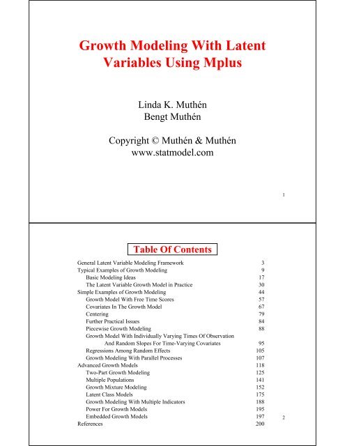
Growth Modeling With Latent Variables Using Mplus - UCLA

Growth Modeling With Latent
Variables Using Mplus
Linda K. Muthén
Bengt Muthén
Copyright © Muthén & Muthén
www.statmodel.com
Table Of Contents
General Latent Variable Modeling Framework
Typical Examples of Growth Modeling
Basic Modeling Ideas
The Latent Variable Growth Model in Practice
Simple Examples of Growth Modeling
Growth Model With Free Time Scores
Covariates In The Growth Model
Centering
Further Practical Issues
Piecewise Growth Modeling
Growth Model With Individually Varying Times Of Observation
And Random Slopes For Time-Varying Covariates
Regressions Among Random Effects
Growth Modeling With Parallel Processes
Advanced Growth Models
Two-Part Growth Modeling
Multiple Populations
Growth Mixture Modeling
Latent Class Models
Growth Modeling With Multiple Indicators
Power For Growth Models
Embedded Growth Models
References
3
9
17
30
44
57
67
79
84
88
95
105
107
118
125
141
152
175
188
195
197
200
1
2

Statistical Analysis With Latent Variables
A General Modeling Framework
Statistical Concepts Captured By Latent Variables
• Continuous Latent Variables
• Measurement errors
• Factors
• Random effects
• Variance components
• Missing data
• Categorical Latent Variables
• Latent classes
• Clusters
• Finite mixtures
• Missing data
Statistical Analysis With Latent Variables
A General Modeling Framework (Continued)
Models That Use Latent Variables
• Continuous Latent Variables • Categorical Latent Variables
• Factor analysis models
• Structural equation models
• Growth curve models
• Multilevel models
• Latent class models
• Mixture models
• Discrete-time survival models
• Missing data models
Mplus integrates the statistical concepts captured by
latent variables into a general modeling framework
that includes not only all of the models listed above
but also combinations and extensions of these models.
3
4

General Latent Variable Modeling Framework
Types of Variables
• Observed variables
x background variables (no model structure)
y continuous and censored outcome variables
u categorical (dichotomous, ordinal, nominal) and
count outcome variables
• Latent variables
f continuous variables
– interactions among f’s
c categorical variables
– multiple c’s
General Latent Variable Modeling Framework
5
6

General Latent Variable Modeling Framework
General Latent Variable Modeling Framework
7
8

Typical Examples Of Growth Modeling
LSAY Data
Longitudinal Study of American Youth (LSAY)
• Two cohorts measured each year beginning in 1987
– Cohort 1 - Grades 10, 11, and 12
– Cohort 2 - Grades 7, 8, 9, and 10
• Each cohort contains approximately 60 schools with
approximately 60 students per school
• Variables - math and science achievement items, math and
science attitude measures, and background variable from
parents, teachers, and school principals
• Approximately 60 items per test with partial item overlap across
grades - adaptive tests
9
10

Math Achievement
Math Achievement
40 50 60 70 80
40 50 60 70 80
Average Score
66
64
62
60
58
56
54
52
50
Math Total Score
LSAY Data
Male Younger
Female Younger
Male Older
Female Older
7 8 9 10
Grade
11 12
LSAY Mean Curve
7 8 9 10
Grade
Individual Curves
7 8 9 10
Grade
11
12

Math Achievement
Math Attitude
40 50 60 70 80
10 11 12 13 14 15
LSAY Sample Means for Math
7 8 9 10
Grade
Sample Means for Attitude Towards Math
7 8 9 10
Grade
Maternal Health Project Data
Maternal Health Project (MHP)
• Mothers who drank at least three drinks a week during
their first trimester plus a random sample of mothers who
used alcohol less often
• Mothers measured at fourth month and seventh month of
pregnancy, at delivery, and at 8, 18, and 36 months
postpartum
• Offspring measured at 0, 8, 18 and 36 months
• Variables for mothers - demographic, lifestyle, current
environment, medical history, maternal psychological
status, alcohol use, tobacco use, marijuana use, other illicit
drug use
• Variables for offspring - head circumference, height,
weight, gestational age, gender, and ethnicity
13
14

MHP: Offspring Head Circumference
Child’s Head Circumference (in millimeters)
500
450
400
350
300
Exposed to Prenatal Alcohol
Average for All Children
0 8 18 36
Child’s Age (in months)
Alternative Models For Longitudinal Data
• Growth curve model
• Auto-regressive model
• Hybrids
15
16

Basic Modeling Ideas
Individual Development Over Time
(1) y it = η 0i + η 1i x t + ε it
i = individual y = outcome
t = timepoint x = time score
η 0 = growth η 1 = growth
intercept slope
y
i = 1
i = 2
i = 3
x
(2a) η 0i = α 0 + γ 0 w i + ζ 0i
(2b) η 1i = α 1 + γ 1 w i + ζ 1i
w = time-invariant covariate
η 0
η 1
w
w
17
18

y
Individual Development Over Time
i = 1
i = 2
i = 3
(1) y it = η 0i + η 1i x t + ε it
(2a) η 0i = α 0 + γ 0 w i + ζ 0i
(2b) η 1i = α 1 + γ 1 w i + ζ 1i
x
t = 1 t = 2 t = 3 t = 4
ε1 ε2 ε3 ε4 Random Effects: Multilevel
And Mixed Linear Modeling
y 1
η 0
w
y 2 y 3 y 4
Individual i (i = 1, 2, …, n) observed at time point t (t = 1, 2, … T).
Multilevel model with two levels (e.g. Raudenbush & Bryk,
2002, HLM).
• Level 1: yit = η0i + η1i xit + κi wit + εit (39)
• Level 2: η0i = α0 + γ0 wi + ζ0i η1i = α1 + γ1 wi + ζ1i κi = α + γ wi + ζ1i Mixed linear model:
(40)
(41)
(42)
yit = fixed part + random part (43)
= α0 + γ0 wi + (α1 + γ1 wi) xit +(α + γ wi) wit (44)
+ ζ0i + ζ1i xit + ζi wit + εit . (45)
η 1
19
20

Random Effects: Multilevel
And Mixed Linear Modeling (Continued)
E.g. “time X w i ” refers to γ 1 (e.g. Rao, 1958; Laird &
Ware, 1982; Jennrich & Sluchter, 1986; Lindstrom & Bates,
1988; BMDP5V; Goldstein, 1995, MLn; SAS PROC MIXED
- Littell et al. 1996 and Singer, 1999).
Random Effects: SEM and
Multilevel Modeling
SEM (Tucker, 1958; Meredith & Tisak, 1990; McArdle &
Epstein 1987; SEM software):
Measurement part:
y it = η 0i + η 1i x t + κ t w it + ε it . (46)
Compare with level 1 of multilevel:
y it = η 0i + η 1i x it + κ i w it + ε it . (47)
Multilevel approach:
• x it as data: Flexible individually-varying times of
observation
• Slopes for time-varying covariates vary over individuals
21
22

Random Effects: SEM and
Multilevel Modeling (Continued)
SEM approach:
• x t as parameters: Flexible growth function form
• Slopes for time-varying covariates vary over time points
Structural part (same as level 2, except for κ t ):
η 0i = α 0 + γ 0 w i + ζ 0it , (48)
η 1i = α 1 + γ 1 w i + ζ 1i , (49)
κ t not involved (parameter).
Random Effects: Mixed
Linear Modeling and SEM
Mixed linear model in matrix form:
y i = (y i1 , y i2 , …, y iT ) ́ (51)
= X i α + Z i b i + e i . (52)
Here, X, Z are design matrices with known values, α contains
fixed effects, and b contains random effects. Compare with
(39) - (43).
23
24

Random Effects: Mixed Linear
Modeling and SEM (Continued)
SEM in matrix form:
y i = v + Λ η i + Κ x i ε i , (53)
η i = α + Β η i + Γ x i + ζ i . (54)
yi = fixed part + random part
= v + Λ (Ι – Β) -1 α + Λ (Ι – Β) -1 Γ xi + Κ xi + Λ (Ι – Β) -1 ζi + εi .
Assume x it = x t , κ i = κ t in (39). Then (39) is handled by
(53) and (40) – (41) are handled by (54), putting x t in Λ and
w it , w i in x i .
Need for Λ i , Κ i , Β i , Γ i .
Comparison Summary of Multilevel,
Mixed Linear, and SEM Growth Models
• Multilevel and mixed linear models are the same
• SEM differs from the multilevel and mixed linear models in two
ways
• Treatment of time scores
• Time scores are data for multilevel and mixed linear
models -- individuals can have different times of
measurement
• Time scores are parameters for SEM growth models -time
scores can be estimated
• Treatment of time-varying covariates
• Time-varying covariates have random effect coefficients
for multilevel and mixed linear models -- coefficients
vary over individuals
• Time-varying covariates have fixed effect coefficients
for SEM growth models -- coefficients vary over time
25
26

Growth Modeling Approached in Two Ways:
Data Arranged As Wide Versus Long
• Wide: Multivariate, Single-Level Approach
y ti = i i + s i x time ti + ε ti
i i regressed on w i
s i regressed on w i
• Long: Univariate, 2-Level Approach (cluster = id)
Within Between
s i
time y
y
i s
Multilevel Modeling in a
Latent Variable Framework
Integrating multilevel and SEM analyses (Asparouhov & Muthén,
2002).
Flexible combination of random effects and other latent variables:
• Multilevel models with random effects (intercepts, slopes)
- Individually-varying times of observation read as data
- Random slopes for time-varying covariates
• SEM with factors on individual and cluster levels
• Models combining random effects and factors, e.g.
- Cluster-level latent variable predictors with multiple indicators
- Individual-level latent variable predictors with multiple indicators
• Special applications
- Random coefficient regression (no clustering; heteroscedasticity)
- Interactions between latent and observed continuous
variables
w
w
i
s
27
28

Advantages of Growth Modeling
in a Latent Variable Framework
• Flexible curve shape
• Individually-varying times of observation
• Random effects (intercepts, slopes) integrated with other
latent variables
• Regressions among random effects
• Multiple processes
• Multiple populations
• Multiple indicators
• Embedded growth models
• Categorical latent variables: growth mixtures
The Latent Variable Growth Model in Practice
29
30

y
Individual Development Over Time
(1) y it = η 0i + η 1i x t + ε it
(2a) η 0i = α 0 + γ 0 w i + ζ 0i
(2b) η 1i = α 1 + γ 1 w i + ζ 1i
Linear Growth Model
i = 1
i = 2
i = 3
x
t = 1 t = 2 t = 3 t = 4
ε1 ε2 ε3 ε4 Specifying Time Scores For
Linear Growth Models
y 1
η 0
w
y 2 y 3 y 4
• Need two latent variables to describe a linear growth
model: Intercept and Slope
Outcome
1 2 3 4
• Equidistant time scores 0 1 2 3
for slope: 0 .1 .2 .3
η 1
Timepoint
31
32

Specifying Time Scores For
Linear Growth Models (Continued)
Outcome
1 2 3 4 5 6 7
Timepoint
• Nonequidistant time scores 0 1 4 5 6
for slope: 0 .1 .4 .5 .6
Model:
Interpretation of the Linear Growth
Factors
y it = η 0i + η 1i x t + ε it , (17)
where in the example t = 1, 2, 3, 4 and xt = 0, 1, 2, 3:
yi1 = η0i + η1i 0 + εi1, η0i = yi1 – εi1, (18)
(19)
yi2 = η0i + η1i 1 + εi2, (20)
yi3 = η0i + η1i 2 + εi3 , (21)
yi4 = η0i + η1i 3 + εi4 , (22)
33
34

Interpretation of the Linear Growth
Factors (Continued)
Interpretation of the intercept growth factor
η 0i (initial status, level):
Systematic part of the variation in the outcome variable at
the time point where the time score is zero.
• Unit factor loadings
Interpretation of the slope growth factor
η 1i (growth rate, trend):
Systematic part of the increase in the outcome variable for a
time score increase of one unit.
• Time scores determined by the growth curve shape.
Interpreting Growth Model Parameters
• Intercept Growth Factor Parameters
• Mean
• Average of the outcome over individuals at the
timepoint with the time score of zero;
• When the first time score is zero, it is the intercept
of the average growth curve, also called initial status
• Variance
• Variance of the outcome over individuals at the
timepoint with the time score of zero, excluding the
residual variance
35
36

Interpreting Growth Model
Parameters (Continued)
• Linear Slope Growth Factor Parameters
• Mean—average growth rate over individuals
• Variance—variance of the growth rate over individuals
• Covariance with Intercept—relationship between
individual intercept and slope values
• Outcome Parameters
• Intercepts—not estimated in the growth model-fixed at
zero to represent measurement invariance
• Residual Variances—time-specific and measurement
error variation
• Residual Covariances—relationships between timespecific
and measurement error sources of variation
across time
Latent Growth Model Parameters
and Sources of Model Misfit
ε 1 ε 2 ε 3 ε 4
y 1 y 2 y 3 y 4
η 0
η 1
37
38

Latent Growth Model Parameters
For Four Time Points
Linear growth over four time points, no covariates.
Free parameters in the H 1 unrestricted model:
• 4 means and 10 variances-covariances
Free parameters in the H 0 growth model:
(9 parameters, 5 d.f.):
• Means of intercept and slope factors
• Variances of intercept and slope factors
• Covariance of intercept and slope factors
• Residual variances for outcomes
Fixed parameters in the H 0 growth model:
• Intercepts of outcomes at zero
• Loadings for intercept factor at one
• Loadings for slope factor at time scores
• Residual covariances for outcomes at zero
Latent Growth Model Sources of Misfit
Sources of misfit:
• Time scores for slope factor
• Residual covariances for outcomes
• Outcome variable intercepts
• Loadings for intercept factor
Model modifications:
• Recommended
– Time scores for slope factor
– Residual covariances for outcomes
• Not recommended
– Outcome variable intercepts
– Loadings for intercept factor
39
40

Latent Growth Model Parameters
For Three Time Points
Linear growth over three time points, no covariates.
Free parameters in the H 1 unrestricted model:
• 3 means and 6 variances-covariances
Free parameters in the H 0 growth model
(8 parameters, 1 d.f.)
• Means of intercept and slope factors
• Variances of intercept and slope factors
• Covariance of intercept and slope factors
• Residual variances for outcomes
Fixed parameters in the H 0 growth model:
• Intercepts of outcomes at zero
• Loadings for intercept factor at one
• Loadings for slope factor at time scores
• Residual covariances for outcomes at zero
η 0
Time-Varying Covariates
η 1
y 1 y 2 y 3 y 4
w a 21 a 22 a 23 a 24
41
42

Alternative Growth Model Parameterizations
Parameterization 1 – for continuous outcomes
yit = 0 + η0i + η1i xt + εit , (32)
η0i = α0 + γ0 wi + ζ0i , (33)
η1i = α1 + γ1 wi + ζ1i . (34)
Parameterization 2 – for categorical outcomes and
multiple indicators
yit = v + η0i + η1i xt + εit , (35)
η0i = 0 + γ0 wi + ζ0i , (36)
η1i = α1 + γ1 wi + ζ1i , (37)
Simple Examples of Growth Modeling
43
44

Steps in Growth Modeling
• Preliminary descriptive studies of the data: means,
variances, correlations, univariate and bivariate
distributions, outliers, etc.
• Determine the shape of the growth curve from theory
and/or data
• Individual plots
• Mean plot
• Consider change in variance across time
• Fit model without covariates using fixed time scores
• Modify model as needed
• Add covariates
LSAY Data
The data come from the Longitudinal Study of American
Youth (LSAY). Two cohorts were measured at four time
points beginning in 1987. Cohort 1 was measured in Grades
10, 11, and 12. Cohort 2 was measured in Grades 7, 8, 9, and
10. Each cohort contains approximately 60 students per
school. The variables measured included math and science
achievement items, math and science attitude measures, and
background information from parents, teachers, and school
principals. There were approximately 60 items per test with
partial item overlap across grades – adaptive tests.
Data for the analysis include the younger females. The
variables include math achievement from Grades 7, 8, 9, and
10 and the background variables of mother’s education and
home resources.
45
46

Math Achievement
Math Achievement
40 50 60 70 80
40 50 60 70 80
LSAY Mean Curve
7 8 9 10
Grade
Individual Curves
7 8 9 10
Grade
Input for LSAY TYPE=BASIC Analysis
TITLE:
DATA:
VARIABLE:
ANALYSIS:
PLOT:
LSAY For Younger Females With Listwise Deletion
TYPE=BASIC Analysis
FILE IS lsay.dat;
FORMAT IS 3F8.0 F8.4 8F8.2 3F8.0;
NAMES ARE cohort id school weight math7 math8 math9
math10 att7 att8 att9 att10 gender mothed homeres;
USEOBS = (gender EQ 1 AND cohort EQ 2);
MISSING = ALL (999);
USEVAR = math7-math10;
TYPE = BASIC;
TYPE = PLOT1; !New in Mplus Version 3
47
48

Sample Statistics for LSAY Data
Sample Statistics
Means
Covariances
MATH7
MATH8
MATH9
MATH10
Correlations
MATH7
MATH8
MATH9
MATH10
MATH7
52.750
MATH7
81.107
67.663
73.150
77.952
MATH7
1.000
0.826
0.808
0.755
n = 984
MATH8
55.411
MATH8
82.829
76.513
82.668
MATH8
1.000
0.837
0.793
MATH9
59.128
MATH9
100.986
95.158
MATH9
1.000
0.826
MATH10
61.796
MATH10
131.326
MATH10
1.000
math7 math8 math9 math10
level trend
49
50

Input For LSAY Linear Growth Model
Without Covariates
TITLE:
DATA:
VARIABLE:
ANALYSIS:
MODEL:
OUTPUT:
LSAY For Younger Females With Listwise Deletion
Linear Growth Model Without Covariates
FILE IS lsay.dat;
FORMAT IS 3F8.0 F8.4 8F8.2 3F8.0;
NAMES ARE cohort id school weight math7 math8 math9
math10 att7 att8 att9 att10 gender mothed homeres;
USEOBS = (gender EQ 1 AND cohort EQ 2);
MISSING = ALL (999);
USEVAR = math7-math10;
TYPE = MEANSTRUCTURE;
level BY math7-math10@1;
trend BY math7@0 math8@1 math9@2 math10@3;
[math7-math10@0];
[level trend];
SAMPSTAT STANDARDIZED MODINDICES (3.84);
!New Version 3 Language For Growth Models
!MODEL: level trend | math7@0 math8@1 math9@2 math10@3;
Output Excerpts LSAY Linear Growth
Model Without Covariates
Tests Of Model Fit
Chi-Square Test of Model Fit
Value 22.664
Degrees of Freedom 5
P-Value 0.0004
CFI/TLI
CFI 0.995
TLI 0.994
RMSEA (Root Mean Square Error Of Approximation)
Estimate 0.060
90 Percent C.I. 0.036 0.086
Probability RMSEA

Output Excerpts LSAY Linear Growth
Model Without Covariates (Continued)
Modification Indices
TREND
TREND
TREND
LEVEL BY
MATH7
MATH8
MATH9
MATH10
TREND BY
MATH7
MATH8
MATH9
MATH10
BY MATH7
BY MATH8
BY MATH9
Model Results
M.I.
6.793
14.694
9.766
1.000
1.000
1.000
1.000
.000
1.000
2.000
3.000
E.P.C.
0.185
-0.169
0.155
.000
.000
.000
.000
.000
.000
.000
.000
Std.E.P.C.
0.254
-0.233
.000
.000
.000
.000
.000
.000
.000
.000
0.213
Output Excerpts LSAY Linear
Growth Without Covariates
StdYX E.P.C.
8.029
8.029
8.029
8.029
.000
1.377
2.753
4.130
0.029
-0.025
0.021
Estimates S.E. Est./S.E. Std StdYX
.906
.861
.800
.708
.000
.148
.274
.364
53
54

Output Excerpts LSAY Linear
Growth Without Covariates (Continued)
LEVEL WITH
TREND
Residual Variances
MATH7
MATH8
MATH9
MATH10
Variances
LEVEL
TREND
Means
LEVEL
TREND
Intercepts
MATH7
MATH8
MATH9
MATH10
Observed
Variable
MATH7
MATH8
MATH9
MATH10
3.491
14.105
13.525
14.726
25.989
64.469
1.895
R-Square
0.820
0.844
0.854
0.798
52.623
3.105
.000
.000
.000
.000
.730
1.253
.866
.989
1.870
3.428
.322
.275
.075
.000
.000
.000
.000
4.780
11.259
15.610
14.897
13.898
18.809
5.894
191.076
41.210
.000
.000
.000
.000
.316
14.105
13.525
14.726
25.989
1.000
1.000
6.554
2.255
.000
.000
.000
.000
.316
.180
.156
.146
.202
1.000
1.000
Output Excerpts LSAY Linear
Growth Without Covariates (Continued)
R-Square
6.554
2.255
.000
.000
.000
.000
55
56

Growth Model With Free Time Scores
Specifying Time Scores For Non-Linear
Growth Models With Estimated Time Scores
Non-Linear Growth Models with Estimated Time scores
• Need two latent variables to describe a non-linear growth
model: Intercept and Slope
Outcome
∗ ∗
1 2 3 4
Timepoint
Outcome
1 2 3 4
Time scores: 0 1 Estimated Estimated
∗
∗
57
Timepoint
58

Interpretation of Slope Growth Factor Mean
For Non-Linear Models
• The slope growth factor mean is the change in the outcome
variable for a one unit change in the time score
• In non-linear growth models, the time scores should be
chosen so that a one unit change occurs between
timepoints of substantive interest.
• An example of 4 timepoints representing grades 7, 8, 9,
and 10
• Time scores of 0 1 * * – slope factor mean refers to
change between grades 7 and 8
• Time scores of 0 * * 1 – slope factor mean refers to
change between grades 7 and 10
Growth Model With Free Time Scores
• Identification of the model – for a model with two growth
factors, at least one time score must be fixed to a non-zero
value (usually one) in addition to the time score that is
fixed at zero (centering point)
• Interpretation—cannot interpret the mean of the slope
growth factor as a constant rate of change over all
timepoints, but as the rate of change for a time score
change of one.
• Approach—fix the time score following the centering point
at one
• Choice of time score starting values if needed
• Means 52.75 55.41 59.13 61.80
• Differences 2.66 3.72 2.67
• Time scores 0 1 >2 >2+1
59
60

Input For LSAY Linear Growth Model
With Free Time Scores Without Covariates
TITLE:
DATA:
VARIABLE:
ANALYSIS:
MODEL:
OUTPUT:
LSAY For Younger Females With Listwise Deletion
Growth Model With Free Time Scores Without Covariates
FILE IS lsay.dat;
FORMAT IS 3F8.0 F8.4 8F8.2 3F8.0;
NAMES ARE cohort id school weight math7 math8 math9
math10 att7 att8 att9 att10 gender mothed homeres;
USEOBS = (gender EQ 1 AND cohort EQ 2);
MISSING = ALL (999);
USEVAR = math7-math10;
TYPE = MEANSTRUCTURE;
level BY math7-math10@1;
trend BY math7@0 math8@1 math9 math10;
[math7-math10@0];
[level trend];
RESIDUAL;
!New Version 3 Language For Growth Models
!MODEL: level trend | math7@0 math8@1 math9 math10;
Output Excerpts LSAY Growth Model
With Free Time Scores Without Covariates
Tests Of Model Fit
n = 984
Chi-Square Test of Model Fit
Value
Degrees of Freedom
P-Value
CFI/TLI
CFI
TLI
RMSEA (Root Mean Square Error Of Approximation)
Estimate
90 Percent C.I.
Probability RMSEA

Output Excerpts LSAY Growth Model
With Free Time Scores Without
Covariates (Continued)
Selected Estimates
LEVEL BY
MATH7
MATH8
MATH9
MATH10
TREND BY
MATH7
MATH8
MATH9
MATH10
TREND WITH
LEVEL
Means
LEVEL
TREND
Estimates S.E. Est./S.E. Std StdYX
1.000
1.000
1.000
1.000
.000
1.000
2.452
3.497
3.110
52.785
2.586
.000
.000
.000
.000
.000
.000
.133
.199
.600
.283
.167
.000
.000
.000
.000
.000
.000
18.442
17.540
5.186
186.605
15.486
8.029
8.029
8.029
8.029
.000
1.377
2.780
3.966
Output Excerpts LSAY Growth Model
With Free Time Scores Without
Covariates (Continued)
Variances
LEVEL
TREND
64.470
1.286
3.394
.265
18.994
4.853
.342
1.000
1.000
6.574
2.280
.903
.870
.797
.708
.000
.148
.276
.350
(Estimates S.E. Est./S.E. Std StdYX)
.342
63
1.000
1.000
6.574
2.280
64

Output Excerpts LSAY Growth Model With Free
Time Scores Without Covariates (Continued)
Residuals
MATH7
MATH8
MATH9
MATH10
Model Estimated Means / Intercepts / Thresholds
MATH7
52.785
MATH7
-.035
MATH8
55.370
MATH8
.041
MATH9
59.123
MATH9
.004
MATH10
61.827
Residuals for Means / Intercepts / Thresholds
79.025
67.580
72.094
75.346
85.180
78.356
82.952
101.588
93.994
MATH10
-.031
Output Excerpts LSAY Growth Model With Free
Time Scores Without Covariates (Continued)
MATH7
MATH8
MATH9
MATH10
Model Estimated Covariances / Correlations / Residual
Correlations
MATH7 MATH8 MATH9 MATH10
1.999
.014
.981
2.527
-2.436
-1.921
-.368
-.705
1.067
128.477
Residuals for Covariances / Correlations / Residual
Correlations
MATH7 MATH8 MATH9 MATH10
2.715
65
66

Covariates In The Growth Model
Covariates In The Growth Model
• Types of covariates
• Time-invariant covariates—vary across individuals not
time, explain the variation in the growth factors
• Time-varying covariates—vary across individuals and
time, explain the variation in the outcomes beyond the
growth factors
67
68

math7 math8 math9 math10
level trend
mothed homeres
Input For LSAY Linear Growth Model
With Free Time Scores Without Covariates
TITLE: LSAY For Younger Females With Listwise Deletion
Growth Model With Free Time Scores and Covariates
DATA: FILE IS lsay.dat;
FORMAT IS 3F8.0 F8.4 8F8.2 3F8.0;
VARIABLE: NAMES ARE cohort id school weight math7 math8 math9
math10 att7 att8 att9 att10 gender mothed homeres;
USEOBS = (gender EQ 1 AND cohort EQ 2);
MISSING = ALL (999);
USEVAR = math7-math10 mothed homeres;
ANALYSIS: TYPE = MEANSTRUCTURE; !ESTIMATOR = MLM;
MODEL: level by math7-math10@1;
trend BY math7@0 math8@1 math9 math10;
[math7-math10@0];
[level trend];
level trend ON mothed homeres;
!New Version 3 Language For Growth Models
!MODEL: level trend | math7@0 math8@1 math9 math10;
! level trend ON mothed homeres;
69
70

Output Excerpts LSAY Growth Model
With Free Time Scores And Covariates
Tests Of Model Fit for ML
n = 935
Chi-Square Test of Model Fit
Value
Degrees of Freedom
P-Value
CFI/TLI
CFI
TLI
RMSEA (Root Mean Square Error Of Approximation)
Estimate
90 Percent C.I.
Probability RMSEA

Output Excerpts LSAY Growth Model
With Free Time Scores And Covariates (Continued)
Selected Estimates For ML
LEVEL ON
MOTHED
HOMERES
TREND ON
MOTHED
HOMERES
LEVEL WITH
TREND
Residual Variances
LEVEL
TREND
Intercepts
LEVEL
TREND
Observed
Variable
MATH7
MATH8
MATH9
MATH10
Latent
Variable
LEVEL
TREND
Estimates S.E. Est./S.E. Std StdYX
2.054
1.376
.103
.149
2.604
53.931
1.134
43.877
1.859
R-Square
0.813
0.849
0.861
0.796
R-Square
.158
.058
.281
.182
.068
.045
.559
2.995
.253
.790
.221
7.322
7.546
1.524
3.334
4.658
18.008
4.488
55.531
8.398
.257
.172
.094
.136
.297
.842
.942
5.484
1.695
.247
.255
.090
.201
.297
.842
.942
5.484
1.695
Output Excerpts LSAY Growth Model
With Free Time Scores And Covariates (Continued)
R-Square
73
74

Model Estimated Average And Individual
Growth Curves With Covariates
Model:
y it = η 0i + η 1i x t + ε it , (23)
η 0i = α 0 + γ 0 w i + ζ 0i , (24)
η 1i = α 1 + γ 1 w i + ζ 1i , (25)
Estimated growth factor means:
Ê(η0i ) = ˆ α 0+
ˆ γ 0w
, (26)
Ê(η1i ) = ˆ α + ˆ γ w . (27)
1
Estimated outcome means:
Ê(y it ) = Ê(η 0i ) + Ê(η 1i ) x t . (28)
Estimated outcomes for individual i :
yˆ it = ˆ η 0i
+ ˆ η1i
xt
where ˆ η and ˆ 0i
η are estimated factor scores. yˆ
1i
it can be
used for prediction purposes.
1
(29)
Model Estimated Means With Covariates
Model estimated means are available using the TECH4 and
RESIDUAL options of the OUTPUT command.
Estimated Intercept Mean = Estimated Intercept +
Estimated Slope (Mothed)*
Sample Mean (Mothed) +
Estimated Slope (Homeres)*
Sample Mean (Homeres)
43.88 + 2.05*2.31 + 1.38*3.11 = 52.9
Estimated Slope Mean = Estimated Intercept +
Estimated Slope (Mothed)*
Sample Mean (Mothed) +
Estimated Slope (Homeres)*
Sample Mean (Homeres)
1.86 + .10*2.31 + .15*3.11 = 2.56
75
76

Model Estimated Means With Covariates
(Continued)
Estimated Outcome Mean at Timepoint t =
Estimated Intercept Mean +
Estimated Slope Mean * (Time Score at Timepoint t)
Estimated Outcome Mean at Timepoint 1 =
52.9 + 2.56 * (0) = 52.9
Estimated Outcome Mean at Timepoint 2 =
52.9 + 2.56 * (1.00) = 55.46
Estimated Outcome Mean at Timepoint 3 =
52.9 + 2.56 * (2.45) = 59.17
Estimated Outcome Mean at Timepoint 4 =
52.9 + 2.56 * (3.50) = 61.86
Outcome
65
60
55
50
Estimated LSAY Curve
7 8 9 10
Grade
77
78

Centering
Centering
• Centering determines the interpretation of the intercept
growth factor
• The centering point is the timepoint at which the time score is
Zero
• A model can be estimated for different centering points
depending on which interpretation is of interest
• Models with different centering points give the same model
fit because they are reparameterizations of the model
• Changing the centering point in a linear growth model with
four timepoints
Timepoints 1 2 3 4
Centering at
Time scores 0 1 2 3 Timepoint 1
-1 0 1 2 Timepoint 2
-2 -1 0 1 Timepoint 3
-3 -2 -1 0 Timepoint 4
79
80

Input For LSAY Growth Model With Free Time
Scores and Covariates Centered At Grade 10
TITLE:
DATA:
VARIABLE:
ANALYSIS:
MODEL:
LSAY For Younger Females With Listwise Deletion
Growth Model With Free Time Scores and Covariates
Centered at Grade 10
FILE IS lsay.dat;
FORMAT IS 3F8.0 F8.4 8F8.2 3F8.0;
NAMES ARE cohort id school weight math7 math8
math9 math10 att7 att8 att9 att10 gender mothed homeres;
USEOBS = (gender EQ 1 AND cohort EQ 2);
MISSING = ALL (999);
USEVAR = math7-math10 mothed homeres;
TYPE = MEANSTRUCTURE;
level by math7-math10@1;
trend BY math7*-3 math8*-2 math9@-1 math10@0;
[math7-math10@0];
[level trend];
level trend ON mothed homeres;
!New Version 3 Language For Growth Models
!MODEL: level trend | math7*-3 math8*-2 math9@-1 math10@0;
! level trend ON mothed homeres;
Output Excerpts LSAY Growth Model With
Free Time Scores And Covariates
Centered At Grade 10
Tests of Model Fit
CHI-SQUARE TEST OF MODEL FIT
n = 935
Value 15.845
Degrees of Freedom 7
P-Value .0265
RMSEA (ROOT MEAN SQUARE ERROR OF APPROXIMATION)
Estimate .037
90 Percent C.I. .012 .061
Probability RMSEA

Output Excerpts LSAY Growth Model With
Free Time Scores And Covariates
Centered At Grade 10 (Continued)
Selected Estimates
LEVEL ON
MOTHED
HOMERES
TREND ON
MOTHED
HOMERES
Estimates S.E. Est./S.E. Std StdYX
2.418
1.903
0.111
0.161
0.353
0.229
0.073
0.049
6.851
8.294
1.521
3.311
Further Practical Issues
0.238
0.187
0.094
0.136
0.229
0.277
0.090
0.201
83
84

Specifying Time Scores For
Quadratic Growth Models
Quadratic Growth Model
y it = η 0i + η 1i x t + η 2i
+ ε it
• Need three latent variables to describe a quadratic growth
model: Intercept, Linear Slope, Quadratic Slope
Outcome
x
2
t
1 2 3 4
Timepoint
• Linear slope time scores: 0 1 2 3
0 .1 .2 .3
• Quadratic slope time scores: 0 1 4 9
0 .01 .04 .09
Specifying Time Scores For Non-Linear
Growth Models With Fixed Time Scores
Non-Linear Growth Models with Fixed Time scores
• Need two latent variables to describe a non-linear growth
model: Intercept and Slope
Growth model with a logarithmic growth curve--ln(t)
Outcome
1 2 3 4
Time scores: 0 0.69 1.10 1.39
Timepoint
85
86

Specifying Time Scores For Non-Linear
Growth Models With Fixed Time Scores (Continued)
Growth model with an exponential growth curve–
exp(t-1) - 1
Outcome
1 2 3 4
Time scores: 0 1.72 6.39 19.09
Timepoint
Piecewise Growth Modeling
87
88

Piecewise Growth Modeling
• Can be used to represent phases of development
• Can be used to capture non-linear growth
• Each piece has its own growth factor(s)
• Each piece can have its own coefficients for covariates
20
15
10
5
0
1 2 3 4 5 6
One intercept growth factor, two slope growth factors
0 1 2 2 2 2 Time scores piece 1
0 0 0 1 2 3 Time scores piece 2
Piecewise Growth Modeling (Continued)
20
15
10
5
0
1 2 3 4 5 6
Two intercept growth factors, two slope growth factors
0 1 2 Time scores piece 1
0 1 2 Time scores piece 2
89
90

TITLE:
DATA:
VARIABLE:
ANALYSIS:
MODEL:
math7 math8 math9 math10
level trend 1 trend 2
Outcome Mean
1 1 2 1 1
7 - 8
& 9 - 10
} Mean of Trend 2
} Mean of Trend 1
7 8 9 10
8 - 9
} Mean of Trend 1
time
Input For LSAY Piecewise Growth Model
With Covariates
LSAY For Younger Females With Listwise Deletion
Piecewise Growth Model With Covariates
FILE IS lsay.dat;
FORMAT IS 3F8.0 F8.4 8F8.2 3F8.0;
NAMES ARE cohort id school weight math7 math8
math9 math10 att7 att8 att9 att10 gender mothed homeres;
USEOBS = (gender EQ 1 AND cohort EQ 2);
MISSING = ALL (999);
USEVAR = math7-math10 mothed homeres;
TYPE = MEANSTRUCTURE;
level BY math7-math10@1;
trend BY math7@0 math8@1 math9@1 math10@2;
trend BY math7@0 math8@0 math9@1 math10@1;
[math7-math10@0];
[level trend1 trend2];
level trend1 trend2 ON mothed homeres;
!New Version 3 Language For Growth Models
!MODEL: level trend1 | math7@0 math8@1 math9@1 math10@2;
! level trend2 | math7@0 math8@0 math9@1 math10@1;
! level trend1 trend2 ON mothed homeres;
91
92

Output Excerpts LSAY Piecewise Growth Model
With Covariates
Tests of Model Fit
CHI-SQUARE TEST OF MODEL FIT
n = 935
Value 11.721
Degrees of Freedom 3
P-Value .0083
RMSEA (ROOT MEAN SQUARE ERROR OF APPROXIMATION)
TREND1 ON
MOTHED
HOMERES
TREND2 ON
MOTHED
HOMERES
Estimate .056
90 Percent C.I. .025 .091
Probability RMSEA

Growth Model With Individually Varying Times
Of Observation And Random Slopes
For Time-Varying Covariates
Growth Modeling In Multilevel Terms
Time point t, individual i (two-level modeling, no clustering):
y ti : repeated measures on the outcome, e.g. math achievement
a 1ti : time-related variable (time scores); e.g. grade 7-10
a 2ti : time-varying covariate, e.g. math course taking
x i : time-invariant covariate, e.g. grade 7 expectations
Two-level analysis with individually-varying times of observation and
random slopes for time-varying covariates:
Level 1: y ti = π 0i + π 1i a 1ti + π 2ti a 2ti + e ti , (55)
Level 2:
π 0i = ß 00 + ß 01 x i + r 0i ,
π 1i = ß 10 + ß 11 x i + r 1i , (56)
π 2i = ß 20 + ß 21 x i + r 2i .
95
96

Growth Modeling In
Multilevel Terms (Continued)
Time scores a 1ti read in as data (not loading parameters).
• π 2ti possible with time-varying random slope variances
• Flexible correlation structure for V (e) = Θ (T x T)
• Regressions among random coefficients possible, e.g.
female
mothed
π 1i = ß 10 + γ 1 π 0i + ß 11 x i + r 1i , (57)
π 2i = ß 20 + γ 2 π 0i + ß 21 x i + r 2i . (58)
homeres
i
s
stvc
math7 math8 math9 math10
crs7
crs8 crs9 crs10
97
98

Input For Growth Model With Individually
Varying Times Of Observation
TITLE:
DATA:
VARIABLE:
growth model with individually varying times of
observation and random slopes
FILE IS lsaynew.dat;
FORMAT IS 3F8.0 F8.4 8F8.2 3F8.0;
NAMES ARE math7 math8 math9 math10 crs7 crs8 crs9
crs10 female mothed homeres a7-a10;
! crs7-crs10 = highest math course taken during each
! grade (0=no course, 1=low, basic, 2=average, 3=high.
! 4=pre-algebra, 5=algebra I, 6=geometry,
! 7=algebra II, 8=pre-calc, 9=calculus)
MISSING ARE ALL (9999);
CENTER = GRANDMEAN (crs7-crs10 mothed homeres);
TSCORES = a7-a10;
Input For Growth Model With Individually
Varying Times Of Observation (Continued)
DEFINE:
ANALYSIS:
MODEL:
OUTPUT:
math7 = math7/10;
math8 = math8/10;
math9 = math9/10;
math10 = math10/10;
TYPE = RANDOM MISSING;
ESTIMATOR = ML;
MCONVERGENCE = .001;
i s | math7-math10 AT a7-a10;
stvc | math7 ON crs7;
stvc | math8 ON crs8;
stvc | math9 ON crs9;
stvc | math10 ON crs10;
i ON female mothed homeres;
s ON female mothed homeres;
stvc ON female mothed homeres;
i WITH s;
stvc WITH i;
stvc WITH s;
TECH8;
99
100

Output Excerpts For Growth Model With
Individually Varying Times Of Observation
And Random Slopes For Time-Varying Covariates
Tests of Model Fit
Loglikelihood
n = 2271
HO Value -8199.311
Information Criteria
Model Results
I ON
FEMALE
MOTHED
HOMERES
S ON
FEMALE
MOTHED
HOMERES
STVC ON
FEMALE
MOTHED
HOMERES
I WITH
S
STVC WITH
I
S
Number of Free Parameters 22
Akaike (AIC) 16442.623
Bayesian (BIC) 16568.638
Sample-Size Adjusted BIC 16498.740
(n* = (n + 2) / 24)
Output Excerpts For Growth Model With Individually
Varying Times Of Observation And Random Slopes
For Time-Varying Covariates (Continued)
Estimates S.E. Est./S.E.
0.187
0.187
0.159
-0.025
0.015
0.019
-0.008
0.003
0.009
0.038
0.011
0.004
0.036
0.018
0.011
0.012
0.006
0.004
0.013
0.007
0.004
0.006
0.005
0.002
5.247
10.231
14.194
-2.017
2.429
4.835
-0.590
0.429
2.167
6.445
2.087
2.033
101
102

Output Excerpts For Growth Model With Individually
Varying Times Of Observation And Random Slopes
For Time-Varying Covariates (Continued)
Intercepts
MTH7
MTH8
MTH9
MTH10
I
S
STVC
Residual Variances
MTH7
MTH8
MTH9
MTH10
I
S
STVC
0.000
0.000
0.000
0.000
4.992
0.417
0.113
0.185
0.178
0.156
0.169
0.570
0.036
0.012
0.000
0.000
0.000
0.000
0.025
0.009
0.010
0.011
0.008
0.008
0.014
0.023
0.003
0.002
Random Slopes
0.000
0.000
0.000
0.000
198.456
47.275
11.416
16.464
22.232
18.497
12.500
25.087
12.064
5.055
• In single-level modeling random slopes ßi describe variation across
individuals i,
yi = αi + ßi xi + εi , (100)
αi = α + ζ0i , (101)
ßi = ß + ζ1i , (102)
Resulting in heteroscedastic residual variances
2
V (yi | xi) = V ( ßi ) x + (103)
i θ
• In two-level modeling random slopes ßj describe variation across
clusters j
yij = aj + ßj xij + εij , (104)
aj = a + ζ0j , (105)
ßj = ß + ζ1j . (106)
A small variance for a random slope typically leads to slow convergence of the
ML-EM iterations. This suggests respecifying the slope as fixed.
Mplus allows random slopes for predictors that are
• Observed covariates
• Observed dependent variables (Version 3)
104
• Continuous latent variables (Version 3)
103

Regressions Among Random Effects
Regressions Among Random Effects
Standard multilevel model (where x t = 0, 1, …, T):
Level – 1: y it = η 0i + η i x t + ε it , (1)
Level – 2a: η 0i = α 0 + γ 0 w i + ζ 0i , (2)
Level – 2b: η 1i = α 1 + γ 1 w i + ζ 1i . (3)
A useful type of model extension is to replace (3) by the regression equation
η 1i = α + βη 0i + γ w i + ζ i . (4)
Example: Blood Pressure (Bloomqvist, 1977)
η 0
w
η 1
η 0
w
η 1
105
106

Growth Modeling With Parallel Processes
Growth Modeling With Parallel Processes
• Estimate a growth model for each process separately
• Determine the shape of the growth curve
• Fit model without covariates
• Modify the model
• Joint analysis of both processes
• Add covariates
107
108

LSAY Data
The data come from the Longitudinal Study of American Youth
(LSAY). Two cohorts were measured at four time points beginning
in 1987. Cohort 1 was measured in Grades 10, 11, and 12. Cohort 2
was measured in Grades 7, 8, 9, and 10. Each cohort contains
approximately 60 schools with approximately 60 students per
school. The variables measured included math and science
achievement items, math and science attitude measures, and
background information from parents, teachers, and school
principals. There were approximately 60 items per test with partial
item overlap across grades—adaptive tests.
Data for the analysis include the younger females. The variables
include math achievement and math attitudes from Grades 7, 8, 9,
and 10 and mother’s education.
Math Achievement
Math Attitude
40 50 60 70 80
11 12 13 14 15
10
LSAY Sample Means for Math
7 8 9 10
Grade
Sample Means for Attitude Towards Math
7 8 9 10
Grade
109
110

mothed
math7 math8 math9
math
level
att
level
math
trend
att
trend
math10
att7 att8 att9 att10
Input For LSAY Parallel Process Growth Model
TITLE:
DATA:
VARIABLE:
ANALYSIS:
LSAY For Younger Females With Listwise Deletion
Parallel Process Growth Model-Math Achievement and
Math Attitudes
FILE IS lsay.dat;
FORMAT IS 3f8 f8.4 8f8.2 3f8 2f8.2;
NAMES ARE cohort id school weight math7 math8 math9
math10 att7 att8 att9 att10 gender mothed homeres
ses3 sesq3;
USEOBS = (gender EQ 1 AND cohort EQ 2);
MISSING = ALL (999);
USEVAR = math7-math10 att7-att10 mothed;
TYPE = MEANSTRUCTURE;
111
112

Input For LSAY Parallel Process Growth Model
MODEL:
OUTPUT
levmath BY math7-math10@1;
trndmath BY math7@0 math8@1 math9 math10;
levatt BY att7-att10@1;
trndatt BY att7@0 att8@1 att9@2 att10@3;
[math7-math10@0 att7-att10@0];
[levmath trndmath levatt trndatt];
levmath-trndatt ON mothed;
MODINDICES STANDARDIZED;
!New Version 3 Language For Growth Models
!MODEL: levmath trndmath | math7@0 math8@1 math9 math10;
! levatt trndatt | att7@0 att8@1 att9@2 att10@3;
! levmath-trndatt ON mothed;
Output Excerpts LSAY Parallel
Process Growth Model
Tests of Model Fit
Chi-Square Test of Model Fit
n = 910
Value 43.161
Degrees of Freedom 24
P-Value .0095
RMSEA (Root Mean Square Error Of Approximation)
Estimate .030
90 Percent C.I. .015 .044
Probability RMSEA

Output Excerpts LSAY Parallel
Process Growth Model (Continued)
Selected Estimates
LEVMATH ON
MOTHED
TRNDMATH ON
MOTHED
LEVATT ON
MOTHED
TRNDATT ON
MOTHED
TRNDATT WITH
LEVMATH
TRNDMATH
LEVATT
Estimates S.E. Est./S.E. Std StdYX
2.462
.145
.053
.012
-.276
.130
-.567
.280
.066
.086
.035
.279
.066
.115
8.798
2.195
.614
.346
-.987
1.976
-4.913
.311
.132
.025
.017
Output Excerpts LSAY Parallel
Process Growth Model (Continued)
Selected Estimates (Continued)
TRNDMATH WITH
LEVMATH
LEVATT WITH
LEVMATH
TRNDMATH
4.733
.544
.702
.164
6.738
3.312
.282
.235
-.049
.168
-.378
.303
.129
.024
.017
Estimates S.E. Est./S.E. Std StdYX
3.032
.580
5.224
.350
.350
115
.282
.235
-.049
.168
-.378
116

Computational Issues For Growth Models
• Decreasing variances of the observed variables over time may make the
modeling more difficult
• Scale of observed variables – keep on a similar scale
• Convergence – often related to starting values or the type of model being
estimated
• Program stops because maximum number of iterations has been reached
• If no negative residual variances, either increase the number of
iterations or use the preliminary parameter estimates as starting values
• If there are large negative residual variances, try better starting values
• Program stops before the maximum number of iterations has been
reached
• Check if variables are on a similar scale
• Try new starting values
• Starting values – the most important parameters to give starting values to are
residual variances and the intercept growth factor mean
• Convergence for models using the | symbol
• Non-convergence may be caused by zero random slope variances which
indicates that the slopes should be fixed rather than random
Advanced Growth Models
117
118

y
Individual Development Over Time
i = 1
i = 2
i = 3
(1) y it = η 0i + η 1i x t + ε it
(2a) η 0i = α 0 + γ 0 w i + ζ 0i
(2b) η 1i = α 1 + γ 1 w i + ζ 1i
x
t = 1 t = 2 t = 3 t = 4
ε1 ε2 ε3 ε4 y 1
η 0
w
y 2 y 3 y 4
Advantages of Growth Modeling
in a Latent Variable Framework
• Flexible curve shape
• Individually-varying times of observation
• Random effects (intercepts, slopes) integrated with other
latent variables
• Regressions among random effects
• Multiple processes
• Multiple populations
• Multiple indicators
• Embedded growth models
• Categorical latent variables: growth mixtures
η 1
119
120

Modeling With A Preponderance Of Zeros
0 1 2 3 4 y 0 1 2 3 4 y
• Outcomes: non-normal continuous – count – categorical
• Censored-normal modeling
• Two-part (semicontinuous modeling): Duan et al. (1983),
Olsen & Schafer (2001)
• Mixture models, e.g. zero-inflated (mixture) Poisson
(Roeder et al., 1999), censored-inflated, mover-stayer
latent transition models, growth mixture models
• Onset (survival) followed by growth: Albert & Shih (2003)
Two-Part (Semicontinuous) Growth Modeling
0 1 2 3 4 y
x c
y1 y2 y3 y4
iy sy
iu
su
u1 u2 u3 u4
121
122

Inflated Growth Modeling
(Two Classes At Each Time Point)
x c
i s
y1 y2 y3 y4
y1#1 y2#1 y3#1 y4#1
ii si
Onset (Survival) Followed By Growth
x
c
y1 y2 y3 y4
iy sy
f
u1
u2 u3 u4
Growth
Event History
123
124

Two-Part Growth Modeling
male
y0
iy
y1 y2 y3
sy
iu su
u0 u1 u2 u3
125
126

Input For Step 1 Of A Two-Part Growth Model
TITLE:
DATA:
VARIABLE:
ANALYSIS:
SAVEDATA:
step 1 of a two-part growth model
Amover u y
>0 1 >0
0 0 999
999 999 999
FILE = amp.dat;
NAMES ARE caseid
amover0 ovrdrnk0 illdrnk0 vrydrn0
amover1 ovrdrnk1 illdrnk1 vrydrn1
amover2 ovrdrnk2 illdrnk2 vrydrn2
amover3 ovrdrnk3 illdrnk3 vrydrn3
amover4 ovrdrnk4 illdrnk4 vrydrn4
amover5 ovrdrnk5 illdrnk5 vrydrn5
amover6 ovrdrnk6 illdrnk6 vrydrn6
tfq0-tfq6 v2 sex race livewith
agedrnk0-agedrnk6 grades0-grades6;
USEV = amover0 amover1 amover2 amover3
sex race u0-u3 y0-y3;
!MISSING = ALL (999);
Input For Step 1 Of A Two-Part Growth Model (Continued)
DEFINE:
u0 = 1; !binary part of variable
IF(amover0 eq 0) THEN u0 = 0;
IF(amover0 eq 999) THEN u0 = 999;
y0 = amover0; !continuous part of variable
IF (amover0 eq 0) THEN y0 = 999;
u1 = 1;
IF(amover1 eq 0) THEN u1 = 0;
IF(amover1 eq 999) THEN u1 = 999:
y1 = amover1;
IF(amover1 eq 0) THEN y1 = 999;
u2 = 1;
IF(amover2 eq 0) THEN u2 = 0;
IF(amover2 eq 999) THEN u2 = 999;
y2 = amover2;
IF(amover2 eq 0) THEN y2 = 999;
u3 = 1;
IF(amover3 eq 0) THEN u3 = 0;
IF(amover3 eq 999) THEN u3 = 999;
y3 = amover3;
IF(amover3 eq 0) THEN y3 = 999;
TYPE = BASIC;
FILE = ampyu.dat;
127
128

Output Excerpts Step 1 Of A Two-Part Growth Model
SAVEDATA Information
Order and format of variables
AMOVER0 F10.3
AMOVER1 F10.3
AMOVER2 F10.3
AMOVER3 F10.3
SEX F10.3
RACE F10.3
U0 F10.3
U1 F10.3
U2 F10.3
U3 F10.3
Y0 F10.3
Y1 F10.3
Y2 F10.3
Y3 F10.3
Save file
ampyu.dat
Save file format
14F10.3
Save file record length 1000
Input For Step 2 Of A Two-Part Growth Model
TITLE:
DATA:
VARIABLE:
DEFINE:
two-part growth model with linear growth for both
parts
FILE = ampyau.dat;
NAMES = amover0-amover3 sex race u0-u3 y0-y3;
USEV = u0-u3 y0-y3 male;
USEOBS = u0 NE 999;
MISSING = ALL (999);
CATEGORICAL = u0-u3;
Male = 2-sex;
129
130

ANALYSIS:
MODEL:
OUTPUT:
PLOT:
Input For Step 2 Of A
Two-Part Growth Model (Continued)
Tests of Model Fit
Loglikelihood
TYPE = MISSING;
ESTIMATOR = ML;
ALGORITHM = INTEGRATION;
COVERAGE = .09;
iu su | u0@0 u1@0.5 u2@1.5 u3@2.5;
iy sy | y0@0 y1@0.5 y2@1.5 y3@2.5;
iu-sy ON male;
! estimate the residual covariances
! iu with su, iy with sy, and iu with iy
iu WITH sy@0;
su WITH iy-sy@0;
PATTERNS SAMPSTAT STANDARDIZED TECH1 TECH4 TECH8;
TYPE = PLOT3;
SERIES = u0-u3(su) | y0-y3(sy);
H0 Value -3277.101
Information Criteria
Output Excerpts Step 2 Of A
Two-Part Growth Model
Number of Free parameters 19
Akaike (AIC) 6592.202
Bayesian (BIC) 6689.444
Sample-Size Adjusted BIC 6629.092
(n* = (n + 2) / 24)
131
132

Output Excerpts Step 2 Of A
Two-Part Growth Model (Continued)
Model Results
IU |
U0
U1
U2
U3
SU |
U0
U1
U2
U3
IY |
Y0
Y1
Y2
Y3
SY |
Y0
Y1
Y2
Y3
Estimates S.E. Est./S.E. Std StdYX
1.000
1.000
1.000
1.000
0.000
0.500
1.500
2.500
1.000
1.000
1.000
1.000
0.000
0.500
1.500
2.500
0.000
0.000
0.000
0.000
0.000
0.000
0.000
0.000
0.000
0.000
0.000
0.000
0.000
0.000
0.000
0.000
0.000
0.000
0.000
0.000
0.000
0.000
0.000
0.000
0.000
0.000
0.000
0.000
0.000
0.000
0.000
0.000
2.839
2.839
2.839
2.839
0.000
0.416
1.249
2.082
Output Excerpts Step 2 Of A
Two-Part Growth Model (Continued)
0.534
0.534
0.534
0.534
0.000
0.117
0.351
0.586
0.843
0.882
0.926
0.905
0.000
0.129
0.407
0.664
0.787
0.738
0.740
0.644
0.000
0.162
0.487
0.707
133
134

Output Excerpts Step 2 Of A
Two-Part Growth Model (Continued)
IU ON
MALE
SU ON
MALE
IY ON
MALE
SY ON
MALE
IU WITH
SU
IY
SY
IY WITH
SY
SU WITH
IY
SY
Intercepts
Y0
Y1
Y2
Y3
IU
SU
IY
SY
Thresholds
U0$1
U1$1
U2$1
U3$1
0.569
-0.181
0.149
-0.068
-1.144
1.193
0.000
-0.039
0.000
0.000
0.000
0.000
0.000
0.000
0.000
0.855
0.232
0.240
2.655
2.655
2.655
2.655
0.234
0.119
0.061
0.038
0.326
0.134
0.000
0.019
0.000
0.000
0.000
0.000
0.000
0.000
0.000
0.098
0.059
0.031
0.206
0.206
0.206
0.206
2.433
-1.518
2.456
-1.790
-3.509
8.897
0.000
-2.109
0.000
0.000
0.000
0.000
0.000
0.000
0.000
8.716
3.901
7.830
12.877
12.877
12.877
12.877
0.200
-0.218
0.279
-0.290
-0.484
0.788
0.000
-0.316
0.000
0.000
0.000
0.000
0.000
0.000
0.000
1.027
0.435
1.025
0.100
-0.109
0.139
-0.145
-0.484
0.788
0.000
-0.316
Output Excerpts Step 2 Of A
Two-Part Growth Model (Continued)
0.000
0.000
135
0.000
0.000
0.000
0.000
0.000
1.027
0.435
1.025
136

Output Excerpts Step 2 Of A
Two-Part Growth Model (Continued)
Residual Variances
Y0
Y1
Y2
Y3
IU
SU
IY
SY
U0
U1
U2
U3
Y0
Y1
Y2
Y3
IU
SU
IY
SY
0.710
0.682
0.650
0.666
0.620
0.491
0.543
0.608
0.010
0.012
0.019
0.021
0.175
0.266
0.238
0.269
7.982
0.685
0.279
0.054
0.032
0.029
0.027
0.054
1.086
0.202
0.040
0.017
5.470
9.159
8.810
5.014
7.351
3.400
7.019
3.224
0.175
0.266
0.238
0.269
0.990
0.988
0.981
0.979
Output Excerpts Step 2 Of A
Two-Part Growth Model (Continued)
R-Square
Observed
Variable
Latent
Variable
R-Square
R-Square
0.380
0.509
0.457
0.392
0.990
0.988
0.981
0.979
137
138

Technical 4 Output
1
IU
SU
IY
SY
MALE
Output Excerpts Step 2 Of A
Two-Part Growth Model (Continued)
IU
SU
IY
SY
MALE
ESTIMATED MEANS FOR THE LATENT VARIABLES
IU
SU
IY SY
0.305
8.062
-1.170
1.214
-0.010
0.142
0.758
0.694
-0.007
0.003
-0.045
0.312
0.285
-0.042
0.037
0.204
0.055
-0.017
MALE
0.536
ESTIMATED COVARIANCE MATRIX FOR THE LATENT VARIABLES
IU
SU
IY SY MALE
1.000
-0.495
0.801
-0.014
0.100
1.000
-0.015
0.016
-0.109
1.000
-0.336
0.139
1.000
-0.145
0.249
Output Excerpts Step 2 Of A
Two-Part Growth Model (Continued)
ESTIMATED CORRELATION MATRIX FOR THE LATENT VARIABLES
IU
SU
IY SY MALE
1.000
139
140

Multiple Populations
Multiple Population Growth Modeling
• Group as a dummy variable
• Multiple-group analysis
• Multiple-group analysis of randomized interventions
141
142

Group Dummy Variable as a Covariate
y 1
η 0
TX
y 2 y 3 y 4
η 1
Two-Group Model
y 1
η 0
y 1
η 0
y 2 y 3 y 4
η 1
y 2 y 3 y 4
η 1
y 5
y 5
y 5
143
144

Birth
Year Cohort
57
58
59
60
61
62
63
64
NLSY: Multiple Cohort Structure
Age a
18 19 20 21 22 23 24 25 26 27 28 29 30 31 32 33 34 35 36 37
82
82 83
82
83
84
82
83
84
85
82
83
84
85
86
82
83
84
85
86
87
82
83
84
85
86
87
88
82
83
84
85
86
87
88
83
84
85
86
87
88
89
84
85
86
87
88
85
86
87
88
86
87
88
87
88
89 90 91 92 93 94
a Non-shaded areas represent years in which alcohol measures were obtained
89
90
89
90
91
89
90
91
92
89
90
91
92
Preventive Interventions
Randomized Trials
Prevention Science Methodology Group (PSMG)
Developmental Epidemiological Framework:
• Determining the levels and variation in risk and protective
factors as well as developmental paths within a defined
population in the absence of intervention
• Directing interventions at these risk and protective factors
in an effort to change the developmental trajectories in a
defined population
• Evaluating variation in intervention impact across risk
levels and contexts on proximal and distal outcomes,
thereby empirically testing the developmental model
93
88
89
90
91
92
93
94
89
90
91
92
93
94
90
91
92
93
94
91
92
93
94
92
93
94
93
94
145
146
94

Aggressive Classroom Behavior:
The GBG Intervention
Muthén & Curran (1997, Psychological Methods)
The Johns Hopkins Prevention Center carried out a schoolbased
preventive intervention randomized trial in Baltimore
public schools starting in grade 1. One of the interventions
tested was the Good Behavior Game intervention, a classroom
based behavior management strategy promoting good
behavior. It was designed specifically to reduce aggressive
behavior of first graders and was aimed at longer term impact
on aggression through middle school.
One first grade classroom in a school was randomly assigned
to receive the Good Behavior Game intervention and another
matched classroom in the school was treated as control. After
an initial assessment in fall of first grade, the intervention was
administered during the first two grades.
The GBG Aggression Example (Continued)
The outcome variable of interest was teacher ratings (TOCA-R) of
each child’s aggressive behavior (Breaks rules, harms property,
fights) in the classroom through grades 1 – 6. Eight teacher ratings
were made from fall and spring for the first two grades and every
spring in grades 3 – 6.
The most important scientific question was whether the Good
Behavior Game reduces the slope of the aggression trajectory
across time. It was also of interest to know whether the intervention
varies in impact for children who started out as high aggressive
versus low aggressive.
Analyses in Muthén-Curran (1997) were based on data for 75 boys
in the GBG group who stayed in the intervention condition for two
years and 111 boys in the control group.
147
148

The GBG Aggression Example:
Analysis Results
Muthén & Curran (1997):
• Step 1: Control group analysis;
• Step 2: Treatment group analysis;
• Step 3: Two-group analysis w/out interactions;
• Step 4: Two-group analysis with interactions;
• Step 5: Sensitivity analysis of final model
• Step 6: Power analysis
TOCA-R
2.9
2.7
2.5
2.3
2.1
1.9
1.7
MUTHÉN AND CURRAN
1.5
1 2 3 4 5 6 7 8 9 10 11 12
Time
Control group: 1/2 ad above mean
Treatment group: 1/2 ad above mean
Control group: At the mean
Treatment group: At the mean
Treatment group: 1/2 ad below mean
Control group: 1/2 ad below mean
Figure 15. Model implied growth trajectories of Teacher Observation of Classroom Behavior—Revised (TOCA-R) scores
as a function of initial status. Each timepoint represents one 6-month interval.
149
150

y1 y2 y3 y4 y5 y6 y7 y8 i s q
y1 y2 y3 y4 y5 y6 y7 y8 i s q
t
Control Group
Growth Mixture Modeling
Treatment Group
151
152

y
Individual Development Over Time
i = 1
i = 2
i = 3
(1) y it = η 0i + η 1i x t + ε it
(2a) η 0i = α 0 + γ 0 w i + ζ 0i
(2b) η 1i = α 1 + γ 1 w i + ζ 1i
x
t = 1 t = 2 t = 3 t = 4
ε1 ε2 ε3 ε4 y 1
η 0
w
y 2 y 3 y 4
Mixtures and Latent Trajectory Classes
Modeling motivated by substantive theories of:
• Multiple Disease Processes: Prostate cancer (Pearson et al.)
• Multiple Pathways of Development: Adolescent-limited versus
life-course persistent antisocial behavior (Moffitt), crime curves
(Nagin), alcohol development (Zucker, Schulenberg)
• Subtypes: Subtypes of alcoholism (Cloninger, Zucker)
η 1
153
154

Example: Mixed-effects Regression Models for
Studying the Natural History of Prostate Disease
Pearson, Morrell, Landis and Carter (1994).
Statistics in Medicine
Outcome
PSA Level (ng/ml)
8
4
0
8
4
0
16
12
8
4
0
Controls
BPH Cases
Local/Regional
Cancers
MIXED-EFFECT REGRESSION MODELS
44
40
36
32
28
24
20
16
12
Metastatic Cancers
15 10 5 0
0
15 10 5 0
Years Before Diagnosis Years Before Diagnosis
8
4
Figure 2. Longitudinal PSA curves estimated from the linear mixed-effects model for the group average (thick
solid line) and for each individual in the study (thin solid lines)
Growth Mixture Modeling
Of Developmental Pathways
Escalating
Early Onset
Normative
Age
x
155
y1 y2 y3 y4
i
c
s
u
q
156

Growth Mixture Modeling
In Randomized Trials
• Growth mixture modeling of control group describing normative
growth
• Class-specific treatment effects in terms of changed trajectories
• Muthén, Brown et al. (2002) in Biostatistics – application to an
aggressive behavior preventive intervention in Baltimore public
schools
TOCA-R
1 2 3 4 5 6
TOCA-R
1 2 3 4 5 6
TOCA-R
1 2 3 4 5 6
TOCA-R
1 2 3 4 5 6
High Class, Control Group
1F 1S 2F 2S 3S 4S 5S 6S 7S
Grades 1-7
Medium Class, Control Group
1F 1S 2F 2S 3S 4S 5S 6S 7S
Grades 1-7
Low Class, Control Group
1F 1S 2F 2S 3S 4S 5S 6S 7S
Grades 1-7
LS Class, Control Group
1F 1S 2F 2S 3S 4S 5S 6S 7S
Grades 1-7
TOCA-R
1 2 3 4 5 6
TOCA-R
1 2 3 4 5 6
TOCA-R
1 2 3 4 5 6
TOCA-R
1 2 3 4 5 6
High Class, Intervention Group
1F 1S 2F 2S 3S 4S 5S 6S 7S
Grades 1-7
Medium Class, Intervention Group
1F 1S 2F 2S 3S 4S 5S 6S 7S
Grades 1-7
Low Class, Intervention Group
1F 1S 2F 2S 3S 4S 5S 6S 7S
Grades 1-7
LS Class, Intervention Group
1F 1S 2F 2S 3S 4S 5S 6S 7S
Grades 1-7
Figure 6. Estimated Mean Growth Curves and Observed Trajectories for
4-Class model 1 by Class and Intervention Status
157
158

Hamilton Depression Rating Scale
0 5 10 15 20 25 30
TOCA-R
TOCA-R
3-Class Model 1
High Class, 14%
Medium Class, 50%
Low Class, 36%
Control
Intervention
1F 1S 2F 2S 3S 4S 5S 6S 7S
Grades 1 - 7
4-Class Model 1
High Class, 15%
Medium Class, 44%
Low Class, 19%
LS Class, 22%
Control
Intervention
1F 1S 2F 2S 3S 4S 5S 6S 7S
Grades 1 - 7
BIC=3421
Entropy=0.83
BIC=3394
Entropy=0.80
A Clinical Trial
of Depression Medication:
2-Class Growth Mixture Modeling
Placebo Non-Responders, 55% Placebo Responders, 45%
Baseline
Wash-in
48 hours
1 week
2 weeks
4 weeks
8 weeks 0
30
25
20
15
10
5
0 5 10 15 20 25 30
Baseline
Wash-in
48 hours
1 week
2 weeks
4 weeks
159
160
5
8 weeks 0
30
25
20
15
10

Mixture Distributions
Non-normality for mixture, normality for mixture components.
1.0
0.8
0.6
0.4
0.2
0.0
1.0
0.8
0.6
0.4
0.2
0.0
Mixture Distribution
0 1 2 3 4 5
Component 1: N(1, .4^2), proportion .75
Component 2: N(2, .8^2), proportion .25
Mixture Components
0 1 2 3 4 5
Two Types of Distribution
(1) Normal mixture components, (2) Preponderance of zeroes (Muthén, 2001, Two-part
growth mixture modeling).
0 20 40 60 80
0 200 400 600 800
SCTAA12F SCTAA15S
0 2 4 6
TFQ2
0 5 10 15
0 20 40 60 80
0 200 400 600 800 1000
0 2 4 6
AMOVER5
-2 -1 0 1 2 3
161
162

Growth Mixture Analysis
Generalization of conventional random effect growth modeling
(multilevel modeling) to include qualitatively different
developments (Muthén & Shedden, 1999 in Biometrics; Muthén
2004 in Handbook chapter).
Combination of conventional growth modeling and cluster analysis
(finite mixture analysis).
• Setting
– Longitudinal data
– A single or multiple items measured repeatedly
– Hypothesized trajectory classes (categorical latent variable)
– Individual trajectory variation within classes
Growth Mixture Analysis
• Aim
– Estimate trajectory shapes
– Estimate trajectory class probabilities
– Estimate variation within class
– Relate class probabilities to covariates
– Classify individuals into classes (posterior prob’s)
– Relate within-class variation to covariates
Application: Mathematics achievement, grades 7 – 10 (LSAY)
related to mother’s education and home resources.
National sample, n = 846.
163
164

A Strategy For Finding The Number Of Classes
In Growth Mixture Modeling
• Comparing models with different numbers of classes
• BIC – low BIC value corresponds to a high loglikelihood
value and a parsimonious model
• TECH11 – Lo-Mendell-Rubin likelihood ratio test
(Biometrika, 2001)
• Residuals and model tests
• TECH7 – class-specific comparisons of model-estimated
means, variances, and covariances versus posterior
probability-weighted sample statistics
• TECH12 – class-mixed residuals for univariate skewness
and kurtosis
• TECH13 – multivariate skew and kurtosis model tests
A Strategy For Finding The Number Of Classes
In Growth Mixture Modeling
• Classification quality
• Posterior probabilities – classification table and entropy
• Individual trajectory classification using pseudo classes
(Bandeen-Roche et al., 1997; Muthén et al. in Biostatistics,
2002)
• Interpretability and usefulness of the latent classes
• Trajectory shapes
• Number of individuals in each class
• Number of estimated parameters
• Substantive theory
• Auxiliary (external) variables – predictive validity
165
166

Strategies For Finding Starting Values In
Growth Mixture Modeling
• Strategy 1
• Do a conventional one-class analysis
• Use estimated growth factor means and standard deviations
as growth factor mean starting values in a multi-class model
– mean plus and minus .5 standard deviation
• Strategy 2
• Estimate a multi-class model with the variances and
covariances of the growth factors fixed to zero
• Use the estimated growth factor means as growth factor
mean starting values for a model with growth factor
variances and covariances free
New in Version 3 – random starts makes it unnecessary to give
starting values: starts = 50 5
Global and Local Solutions
Log likelihood Log likelihood
Parameter Parameter
Log likelihood Log likelihood
Parameter Parameter
167
168

Number of
Classes
Loglikelihood
# parameters
BIC
AIC
Entropy
LRT p-value
for k-1 classes
Multivariate
skew p-value
Multivariate
kurtosis
p-value
c
math7
i
math8 math9 math10
s
mothed homeres
Deciding On The Number Of Classes
For The LSAY Growth Mixture Model
1
-11,997.653
15
24,098
24,025
NA
NA
.00
.00
n = 935
2
-11,864.826
29
23,928
23,788
.468
.0000
.34
.10
3
-11,856.220
36
23,959
23,784
.474
.4041
.26
.05
169
170

BIC
29500
29000
28500
28000
27500
27000
26500
26000
25500
25000
Model Fit by BIC: LSAY
Growth Mixture with Fixed Growth Factor
(Co)Variance = 0
Growth Mixture with Free Growth Factor
(Co)Variance (Invariant Psi and Theta)
Growth Mixture with Free Growth Factor
(Co)Variance (Non-invariant Psi and Theta)
Growth Mixture with Free Growth Factor
(Co)Variance (Non-invariant Psi and Theta,
with 2 Covariates)
1 2 3 4 5 6 7 8
Number of Classes
LSAY: Estimated Two-Class
Growth Mixture Model
y
Class 1
Intercept ON Mothed* Homeres
Slope ON Mothed Homeres*
Class 2
Intercept ON Mothed* Homeres*
Slope ON Mothed Homeres
Conventional Single-Class Analysis
Intercept ON Mothed* Homeres*
Slope ON Mothed Homeres*
Class 2
Class 1
(42%)
t
171
172

TITLE:
DATA:
VARIABLE:
ANALYSIS:
MODEL:
Input For LSAY 2-Class
Growth Mixture Model
2-class varying slopes on mothed and homeres
varying Psi varying Theta
FILE IS lsay.dat;
FORMAT is 3f8 f8.4 8f8.2 2f8.2;
NAMES ARE cohort id school weight math7
math8 math9 math10 att7 att8 att9 att10 gender mothed
homeres;
USEOBS = (gender EQ 1 AND cohort EQ 2);
MISSING = ALL (999);
USEVAR = math7-math10 mothed homeres;
CLASSES = c(2);
TYPE = MIXTURE;
Input For LSAY 2-Class
Growth Mixture Model (Continued)
MODEL: %OVERALL%
intercpt BY math7-math10@1;
slope BY math7@0 math8@1 math9 math10;
[math7-math10@0];
intercpt slope ON mothed homeres;
%c#1%
!Not needed in Version 3
[intercpt*42.8 slope*.6];
!Not needed in Version 3
%c#2%
[intercpt*62.8 slope*3.6];
!Not needed in Version 3
intercpt slope ON mothed homeres;
math7-math10 intercpt slope;
slope WITH intercpt;
OUTPUT: TECH8 TECH11 TECH12 TECH13 RESIDUAL;
New Version 3 Language For Growth Models
%OVERALL%
intercpt slope | math7@0 math8@1 math9 math10;
intercpt slope ON mothed homeres;
%c#2%
intercpt slope ON mothed homeres;
math7-math10 intercpt slope;
slope WITH intercpt;
173
174

Item u1
Item Profiles
Item u2
Item u3
Latent Class Models
Latent Class Analysis
Item u4
Class 1
Class 2
Class 3
Class 4
u1
u2 u3 u4
c
x
175
176

Introduced by Goodman (1974); Bartholomew (1987).
Special case for longitudinal data: latent transition analysis,
introduced by Collins; latent Markov models.
• Setting
Confirmatory Latent Class Analysis
With Several Latent Class Variables
– Cross-sectional or longitudinal data
– Multiple items measuring several different constructs
– Hypothesized simple structure for measurements
– Hypothesized constructs represented as latent class variables
(categorical latent variables)
Confirmatory Latent Class Analysis
With Several Latent Class Variables (Continued)
• Aim
– Identify items that indicate classes well
– Test simple measurement structure
– Study relationships between latent class variables
– Estimate class probabilities
– Relate class probabilities to covariates
– Classify individuals into classes (posterior probabilities)
• Applications
– Latent transition analysis with four latent class indicators at
two time points and a covariate
177
178

Latent Transition Analysis
Transition Probabilities Time Point 1 Time Point 2
c1
1
2
TITLE:
DATA:
VARIABLE:
ANALYSIS:
MODEL:
c2
1 2
0.8 0.2
0.4 0.6
u11 u12 u13 u14 u21 u22 u23 u24
Input For LTA With
Two Time Points And A Covariate
Latent transition analysis for two time points and a
covariate using Mplus Version 3
FILE = mc2tx.dat;
NAMES ARE u11-u14 u21-u24 x c1 c2;
USEV = u11-u14 u21-u24 x;
CATEGORICAL = u11-u24;
CLASSES = c1(2) c2(2);
TYPE = MIXTURE;
%OVERALL%
c2#1 ON c1#1 x;
c1#1 on x;
c1
x
c2
179
180

Input For LTA With
Two Time Points And A Covariate (Continued)
MODEL c1:
MODEL c2:
OUTPUT:
%c1#1%
[u11$1] (1);
[u12$1] (2);
[u13$1] (3);
[u14$1] (4);
%c1#2%
[u11$1] (5);
[u12$1] (6);
[u13$1] (7);
[u14$1] (8);
%c2#1%
[u21$1] (1);
[u22$1] (2);
[u23$1] (3);
[u24$1] (4);
%c2#2%
[u21$1] (5);
[u22$1] (6);
[u23$1] (7);
[u24$1] (8);
TECH1 TECH8;
Tests Of Model Fit
Output Excerpts LTA With
Two Time Points And A Covariate
Loglikelihood
HO Value -3926.187
Information Criteria
Number of Free Parameters 13
Akaike (AIC) 7878.374
Bayesian (BIC) 7942.175
Sample-Size Adjusted BIC 7900.886
(n* = (n + 2) / 24)
Entropy 0.902
181
182

Output Excerpts LTA With
Two Time Points And A Covariate (Continued)
Chi-Square Test of Model Fit for the Latent Class Indicator Model
Part
Pearson Chi-Square
Final Class Counts
Value 250.298
Degrees of Freedom 244
P-Value 0.3772
Likelihood Ratio Chi-Square
Value 240.811
Degrees of Freedom 244
P-Value 0.5457
FINAL CLASS COUNTS AND PROPORTIONS OF TOTAL SAMPLE SIZE BASED
ON ESTIMATED POSTERIOR PROBABILITIES
Class 1
Class 2
Class 3
Class 4
328.42644
184.43980
146.98726
340.14650
0.32843
0.18444
0.14699
0.34015
Output Excerpts LTA With
Two Time Points And A Covariate (Continued)
Model Results
LATENT CLASS INDICATOR MODEL PART
Class 1-C1, 1-C2
Thresholds
U11$1
U12$1
U13$1
U14$1
U21$1
U22$1
U23$1
U24$1
Estimates S.E. Est./S.E.
-2.020
-2.003
-1.776
-1.861
-2.020
-2.003
-1.776
-1.861
0.110
0.106
0.098
0.101
0.110
0.106
0.098
0.101
-18.353
-18.919
-18.046
-18.396
-18.353
-18.919
-18.046
-18.396
183
184

Output Excerpts LTA With
Two Time Points And A Covariate (Continued)
Class 1-C1, 2-C2
Thresholds
U11$1
U12$1
U13$1
U14$1
U21$1
U22$1
U23$1
U24$1
Class 2-C1, 1-C2
Thresholds
U11$1
U12$1
U13$1
U14$1
U21$1
U22$1
U23$1
U24$1
-2.020
-2.003
-1.776
-1.861
1.964
2.164
1.864
2.107
1.964
2.164
1.864
2.107
-2.020
-2.003
-1.776
-1.861
0.110
0.106
0.098
0.101
0.111
0.119
0.100
0.112
0.111
0.119
0.100
0.112
0.110
0.106
0.098
0.101
-18.353
-18.919
-18.046
-18.396
17.736
18.113
18.704
18.879
17.736
18.113
18.704
18.879
-18.353
-18.919
-18.046
-18.396
Output Excerpts LTA With
Two Time Points And A Covariate (Continued)
Model Results (Continued)
Class 2-C1, 2-C2
Thresholds
U11$1
U12$1
U13$1
U14$1
U21$1
U22$1
U23$1
U24$1
Estimates S.E. Est./S.E.
1.964
2.164
1.864
2.107
1.964
2.164
1.864
2.107
0.111
0.119
0.100
0.112
0.111
0.119
0.100
0.112
17.736
18.113
18.704
18.879
17.736
18.113
18.704
18.879
185
186

Output Excerpts LTA With
Two Time Points And A Covariate (Continued)
LATENT CLASS REGRESSION MODEL PART
C2#1 ON
C1#1
C2#1 ON
X
C1#1 ON
X
Intercepts
C1#1
C2#1
0.530
-1.038
-1.540
0.065
-0.407
0.180
0.107
0.112
0.082
0.120
2.953
-9.703
-13.761
0.797
-3.381
Growth Modeling With Multiple Indicators
187
188

Growth Of Latent Variable Construct
Measured By Multiple Indicators
η 0
Steps in Growth Modeling
With Multiple Indicators
• Exploratory factor analysis of indicators for each timepoint
• Determine the shape of the growth curve for each indicator
and the sum of the indicators
• Fit a growth model for each indicator—must be the same
• Confirmatory factor analysis of all timepoints together
• Covariance structure analysis without measurement
parameter invariance
• Covariance structure analysis with invariant loadings
• Mean and covariance structure analysis with invariant
measurement intercepts and loadings
• Growth model with measurement invariance across
timepoints
η 1
189
190

Advantages Of Using Multiple Indicators
Instead Of An Average
• Estimation of unequal weights
• Partial measurement invariance—changes across time in
individual item functioning
• No confounding of time-specific variance and
measurement error variance
• Smaller standard errors for growth factor parameters (more
power)
Classroom Aggression Data (TOCA)
The classroom aggression data are from an intervention study
in Baltimore public schools carried out by the Johns Hopkins
Prevention Research Center. Subjects were randomized into
treatment and control conditions. The TOCA-R instrument
was used to measure 10 aggression items at multiple
timpoints. The TOCA-R is a teacher rating of student
behavior in the classroom. The items are rated on a six-point
scale from almost never to almost always.
Data for this analysis include the 342 boys in the control
group. Four time points are examined: Spring Grade 1, Spring
Grade 2, Spring Grade 3, and Spring Grade 4.
Seven aggression items are used in the analysis:
- Break rules - Lies - Yells at others
- Fights - Stubborn
- Harms others - Teasing classmates
191
192

Degrees Of Invariance Across Time
• Case 1
• Same items
• All items invariant
• Same construct
• Case 2
• Same items
• Some items non-invariant
• Same construct
• Case 3
• Different items
• Some items invariant
• Same construct
• Case 4
• Different items
• Some items invariant
• Different construct
a1 b1 c1 a2 b2 d2 a3 e1 d3 f4 e4 d4
1 λ2 λ3 1 λ2 λ4 1 λ5 λ4 λ6 λ5 λ4
i s
a1 a2 b2 a3 b3
b4
i s
193
194

Power For Growth Models
Designing Future Studies: Power
• Computing power for growth models using Satorra-
Saris (Muthén & Curran, 1997; examples)
• Computing power using Monte Carlo studies (Muthén
& Muthén, 2002)
• Power calculation web site – PSMG
• Multilevel power (Miyazaki & Raudenbush, 2000;
Moerbeek, Breukelen & Berger, 2000; Raudenbush,
1997; Raudenbush & Liu, 2000)
• School-based studies (Brown & Liao, 1999: Principles
for designing randomized preventive trials)
• Multiple- (sequential-) cohort power
• Designs for follow-up (Brown, Indurkhia, Kellam,
2000)
195
196

grade 7 parent & peer
academic push
Embedded Growth Models
female
f
mothed
homeres
i
s
stvc
math7 math8 math9
mthcrs7
math10
mthcrs8 mthcrs9 mthcrs10
197
198

advp advm1 advm2 advm3 momalc2 momalc3
0 0 0 0 0 0
i s
gender ethnicity
hi hs1 hs2
hcirc0 hcirc8 hcirc18 hcirc36
References
(To request a Muthén paper, please email bmuthen@ucla.edu.)
Analysis With Longitudinal Data
Introductory
Collins, L.M. & Sayer, A. (Eds.) (2001). New Methods for the Analysis of
Change. Washington, D.C.: American Psychological Association.
Curran, P.J. & Bollen, K.A. (2001). The best of both worlds: Combining
autoregressive and latent curve models. In Collins, L.M. & Sayer, A.G.
(Eds.) New Methods for the Analysis of Change (pp. 105-136).
Washington, DC: American Psychological Association.
Duncan, T.E., Duncan, S.C., Strycker, L.A., Li, F., & Alpert, A. (1999). An
Introduction to Latent Variable Growth Curve Modeling: Concepts, Issues,
and Applications. Mahwah, NJ: Lawrence Erlbaum Associates.
Goldstein, H. (1995). Multilevel statistical models. Second edition. London:
Edward Arnold.
Jennrich, R.I. & Schluchter, M.D. (1986). Unbalanced repeated-measures
models with structured covariance matrices. Biometrics, 42, 805-820.
199
200

References (Continued)
Khoo, S.T. & Muthén, B. (2000). Longitudinal data on families: Growth
modeling alternatives. In Multivariate Applications in Substance use
Research, . Rose, L. Chassin, C. Presson & J. Sherman (eds.), Hillsdale,
N.J.: Erlbaum, pp. 43-78.
Laird, N.M., & Ware, J.H. (1982). Random-effects models for longitudinal
data. Biometrics, 38, 963-974.
Lindstrom, M.J. & Bates, D.M. (1988). Newton-Raphson and EM algorithms
for linear mixed-effects models for repeated-measures data. Journal of the
American Statistical Association, 83, 1014-1022.
Littell, R., Milliken, G.A., Stroup, W.W., & Wolfinger, R.D. (1996). SAS
system for mixed models. Cary NC: SAS Institute.
McArdle, J.J. & Epstein, D. (1987). Latent growth curves within
developmental structural equation models. Child Development, 58, 110-
133.
McArdle, J.J. & Hamagami, F. (2001). Latent differences score structural
models for linear dynamic analyses with incomplete longitudinal data. In
Collins, L.M. & Sayer, A. G. (Eds.), New Methods for the Analysis of
Change (pp. 137-175). Washington, D.C.: American Psychological
Association.
References (Continued)
Meredith, W. & Tisak, J. (1990). Latent curve analysis Psychometrika, 55,
107-122.
Muthén, B. (1991). Analysis of longitudinal data using latent variable models
with varying parameters. In L. Collins & J. Horn (Eds.), Best Methods for
the Analysis of Change. Recent Advances, Unanswered Questions, Future
Directions (pp. 1-17). Washington D.C.: American Psychological
Association.
Muthén, B. (1997). Latent variable modeling with longitudinal and multilevel
data. In A. Raftery (ed), Sociological Methodology (pp. 453-380). Boston:
Blackwell Publishers.
Muthén, B. (2000). Methodological issues in random coefficient growth
modeling using a latent variable framework: Applications to the
development of heavy drinking. In Multivariate Applications in Substance
use Research, J. Rose, L. Chassin, C. Presson & J. Sherman (eds.),
Hillsdale, N.J.: Erlbaum, pp. 113-140.
Muthén, B. & Curran, P. (1997). General longitudinal modeling of individual
differences in experimental designs: A latent variable framework for
analysis and power estimation. Psychological Methods, 2, 371-402.
201
202

References (Continued)
Muthén, B. & Khoo, S.T. (1998). Longitudinal studies of achievement growth
using latent variable modeling. Learning and Individual Differences.
Special issue: latent growth curve analysis, 10, 73-101.
Muthén, B. & Muthén, L. (2000). The development of heavy drinking and
alcohol-related problems from ages 18 to 37 in a U.S. national sample.
Journal of Studies on Alcohol, 61, 290-300.
Muthén, B. & Shedden, K. (1999). Finite mixture modeling with mixture
outcomes using the EM algorithm. Biometrics, 55, 463-469.
Rao, C.R. (1958). Some statistical models for comparison of growth curves.
Biometrics, 14, 1-17.
Raudenbush, S.W. & Bryk, A.S. (2002). Hierarchical linear models:
Applications and data analysis methods. Second edition. Newbury Park,
CA: Sage Publications.
Singer, J.D. (1998). Using SAS PROC MIXED to fit multilevel models,
hierarchical models, and individual growth models. Journal of Educational
and Behavioral Statistics, 23, 323-355.
Singer, J.D. & Willett, J.B. (2003). Applied longitudinal data analysis.
Modeling change and event occurrence. New York, NY: Oxford University
203
Press.
References (Continued)
Snijders, T. & Bosker, R. (1999). Multilevel analysis: An introduction to basic
and advanced multilevel modeling. Thousand Oakes, CA: Sage
Publications.
Tucker, L.R. (1958). Determination of parameters of a functional relation by
factor analysis. Psychometrika, 23, 19-23.
Advanced
Albert, P.A., McShane, L.M., Shih, J.H. & The US SCI Bladder Tumor
Marker Network (2001). Latent class modeling approaches for assessing
diagnostic error without a gold standard: With applications to p.53
immunohistochemical assays in bladder tumors. Biometrics, 57, 610-619.
Brown, C.H. & Liao, J. (1999). Principles for designing randomized preventive
trials in mental health: An emerging development epidemiologic
perspective. American Journal of Community Psychology, special issue on
prevention science, 27, 673-709.
Brown, C.H., Indurkhya, A. & Kellam, S.K. (2000). Power calculations for
data missing by design: applications to a follow-up study of lead exposure
and attention. Journal of the American Statistical Association, 95, 383-395.
204

References (Continued)
Collins, L.M. & Sayer, A. (Eds.), New Methods for the Analysis of Change.
Washington, D.C.: American Psychological Association.
Duan, N., Manning, W.G., Morris, C.N. & Newhouse, J.P. (1983). A
comparison of alternative models for the demand for medical care. Journal
of Business and Economic Statistics, 1, 115-126.
Ferrer, E. & McArdle, J.J. (2004). Alternative structural models for
multivariate longitudinal data analysis. Structural Equation Modeling, 10,
493-524.
Khoo, S.T. & Muthén, B. (2000). Longitudinal data on families: Growth
modeling alternatives. In Multivariate Applications in Substance use
Research, J. Rose, L. Chassin, C. Presson & J. Sherman (eds), Hillsdale,
N.J.: Erlbaum, pp. 43-78.
Miyazaki, Y. & Raudenbush, S.W. (2000). A test for linkage of multiple
cohorts from an accelerated longitudinal design. Psychological Methods, 5,
44-63.
Moerbeek, M., Breukelen, G.J.P. & Berger, M.P.F. (2000). Design issues for
experiments in multilevel populations. Journal of Educational and
Behavioral Statistics, 25, 271-284.
References (Continued)
Muthén, B. (1996). Growth modeling with binary responses. In A.V. Eye & C.
Clogg (eds), Categorical Variables in Developmental Research: Methods of
Analysis (pp. 37-54). San Diego, CA: Academic Press.
Muthén, B. (1997). Latent variable modeling with longitudinal and multilevel
data. In A. Raftery (ed), Sociological Methodology (pp. 453-380). Boston:
Blackwell Publishers.
Muthén, B. (2004). Latent variable analysis: Growth mixture modeling and
related techniques for longitudinal data. In D. Kaplan (ed.), Handbook of
quantitative methodology for the social sciences (pp. 345-368). Newbury
Park, CA: Sage Publications.
Muthén, B. & Curran, P. (1997). General longitudinal modeling of individual
differences in experimental designs: A latent variable framework for
analysis and power estimation. Psychological Methods, 2, 371-402.
Muthén, B. & Muthén, L. (2000). The development of heavy drinking and
alcohol-related problems from ages 18 to 37 in a U.S. national sample.
Journal of Studies on Alcohol, 61, 290-300.
205
206

References (Continued)
Muthén, L.K. and Muthén, B. O. (2002). How to use a Monte Carlo study to
decide on sample size and determine power. Structural Equation Modeling,
4, 599-620.
Olsen, M.K. & Schafer, J.L. (2001). A two-part random effects model for
semicontinuous longitudinal data. Journal of the American Statistical
Association, 96, 730-745.
Raudenbush, S.W. (1997). Statistical analysis and optimal design for cluster
randomized trials. Psychological Methods, 2, 173-185.
Raudenbush, S.W. & Liu, X. (2000). Statistical power and optimal design for
multisite randomized trials. Psychological Methods, 5, 199-213.
Roeder, K., Lynch, K.G., & Nagin, D.S. (1999). Modeling uncertainty in latent
class membership: A case study in criminology. Journal of the American
Statistical Association, 94, 766-776.
Satorra, A. & Saris, W. (1985). Power of the likelihood ratio test in covariance
structure analysis. Psychometrika, 51, 83-90.
Mixture References
References (Continued)
Analysis With Categorical Latent Variables (Mixture Modeling)
General
Agresti, A. (1990). Categorical data analysis. New York: John Wiley & Sons.
Everitt, B.S. & Hand, D.J. (1981). Finite mixture distributions. London:
Chapman and Hall.
McLachlan, G.J. & Peel, D. (2000). Finite mixture models. New York: Wiley
& Sons.
Muthén, L.K. & Muthén, B. (1998-2001). Mplus User’s Guide. Los Angeles,
CA: Muthén & Muthén.
Schwartz, G. (1978). Estimating the dimension of a model. The Annals of
Statistics, 6, 461-464.
Titterington, D.M., Smith, A.F.M., & Makov, U.E. (1985). Statistical analysis
of finite mixture distributions. Chichester, U.K.: John Wiley & Sons.
Lo, Y., Mendell, N.R. & Rubin, D.B. (2001). Testing the number of
components in a normal mixture. Biometrika, 88, 767-778.
207
208

References (Continued)
Vuong, Q.H. (1989). Likelihood ratio tests for model selection and non-nested
hypotheses. Econometrica, 57, 307-333.
Asparouhov, T. & Muthén, B. (2002). Skew and kurtosis tests in mixture
modeling.
Latent Class Analysis
Bandeen-Roche, K., Miglioretti, D.L., Zeger, S.L. & Rathouz, P.J. (1997).
Latent variable regression for multiple discrete outcomes. Journal of the
American Statistical Association, 92, 1375-1386.
Bartholomew, D.J. (1987). Latent variable models and factor analysis. New
York: Oxford University Press.
Bucholz, K.K., Heath, A.C., Reich, T., Hesselbrock, V.M., Kramer, J.R.,
Nurnberger, J.I., & Schuckit, M.A. (1996). Can we subtype alcoholism? A
latent class analysis of data from relatives of alcoholics in a multi-center
family study of alcoholism. Alcohol Clinical Experimental Research, 20,
1462-1471.
Clogg, C.C. (1995). Latent class models. In G. Arminger, C.C. Clogg & M.E.
Sobel (eds.), Handbook of statistical modeling for the social and behavioral
sciences (pp 331-359). New York: Plenum Press.
References (Continued)
Clogg, C.C. & Goodman, L.A. (1985). Simultaneous latent structural analysis
in several groups. In Tuma, N.B. (ed.), Sociological Methodology, 1985
(pp. 18-110). San Francisco: Jossey-Bass Publishers.
Dayton, C.M. & Macready, G.B. (1988). Concomitant variable latent class
models. Journal of the American Statistical Association, 83, 173-178.
Formann, A.K. (1992). Linear logistic latent class analysis for polytomous
data. Journal of the American Statistical Association, 87, 476-486.
Goodman, L.A. (1974). Exploratory latent structure analysis using both
identifiable and unidentifiable models. Biometrika, 61, 215-231.
Hagenaars, J.A. & McCutcheon, A.L. (2002). Applied latent class analysis.
Cambridge, UK: Cambridge University Press.
Heijden, P.G.M., Dressens, J. & Bockenholt, U. (1996). Estimating the
concomitant-variable latent-class model with the EM algorithm. Journal of
Educational and Behavioral Statistics, 21, 215-229.
Lazarsfeld, P.F. & Henry, N.W. (1968). Latent structure analysis. New York:
Houghton Mifflin.
Muthén, B. (2001). Latent variable mixture modeling. In G.A. Marcoulides &
R.E. Schumacker (eds.), New Developments and Techniques in Structural
Equation Modeling (pp. 1-33). Lawrence Erlbaum Associates.
209
210

References (Continued)
Muthén, B. & Muthén, L. (2000). Integrating person-centered and variablecentered
analysis: growth mixture modeling with latent trajectory classes.
Alcoholism: Clinical and Experimental Research, 24, 882-891.
Nestadt, G., Hanfelt, J., Liang, K.Y., Lamacz, M., Wolyniec, P., Pulver, A.E.
(1994). An evaluation of the structure of schizophrenia spectrum
personality disorders. Journal of Personality Disorders, 8, 288-298.
Rindskopf, D. (1990). Testing developmental models using latent class
analysis. In A. von Eye (ed.), Statistical methods in longitudinal research:
Time series and categorical longitudinal data (Vol 2, pp. 443-469). Boston:
Academic Press.
Rindskopf, D., & Rindskopf, W. (1986). The value of latent class analysis in
medical diagnosis. Statistics in Medicine, 5, 21-27.
Stoolmiller, M. (2001). Synergistic interaction of child manageability problems
and parent-discipline tactics in predicting future growth in externalizing
behavior for boys. Developmental Psychology, 37, 814-825.
Uebersax, J.S., & Grove, W.M. (1990). Latent class analysis of diagnostic
agreement. Statistics in Medicine, 9, 559-572.
Latent Transition Analysis
References (Continued)
Collins, L.M. & Wugalter, S.E. (1992). Latent class models for stagesequential
dynamic latent variables. Multivariate Behavioral Research, 27,
131-157.
Collins, L.M., Graham, J.W., Rouscult, S.S., & Hansen, W.B. (1997). Heavy
caffeine use and the beginning of the substance use onset process: An
illustration of latent transition analysis. In K. Bryant, M. Windle, & S. West
(Eds.), The Science of Prevention: Methodological Advances from Alcohol
and Substance Use Research. Washington DC: American Psychological
Association. pp. 79-99.
Graham, J.W., Collins, L.M., Wugalter, S.E., Chung, N.K., & Hansen, W.B.
(1991). Modeling transitions in latent stage- sequential processes: A
substance use prevention example. Journal of Consulting and Clinical
Psychology, 59, 48-57.
Kandel, D.B., Yamaguchi, K., & Chen, K. (1992). Stages of progression in
drug involvement from adolescence to adulthood: Further evidence for the
gateway theory. Journal of Studies of Alcohol, 53, 447-457.
Reboussin, B.A., Reboussin, D.M., Liang, K.Y., & Anthony, J.C. (1998).
Latent transition modeling of progression of health-risk behavior.
Multivariate Behavioral Research, 33, 457-478.
211
212

Noncompliance (CACE)
References (Continued)
Angrist, J.D., Imbens, G.W., Rubin. D.B. (1996). Identification of causal
effects using instrumental variables. Journal of the American Statistical
Association, 91, 444-445.
Jo, B. (1999). Estimation of intervention effects with noncompliance:
Alternative model specifications. Forthcoming in Journal of Educational
and Behavioral Statistics (will appear with comments).
Jo, B. (2002). Statistical power in randomized intervention studies with
noncompliance. Psychological Methods, 7, 178-193.
Jo, B. (2002). Model misspecification sensitivity analysis in estimating causal
effects of interventions with noncompliance. Statistics in Medicine.
Jo, B. & Muthén, B. (2000). Longitudinal studies with intervention and
noncompliance: Estimation of casual effects in growth mixture modeling.
To appear in N. Duan and S. Reise (Eds.), Multilevel Modeling:
Methodological Advances, Issues, and Applications, Multivariate
Applications Book Series, Lawrence Erlbaum Associates.
Jo, B. & Muthén, B. (2001). Modeling of intervention effects with
noncompliance: A latent variable approach for randomized trials. In G.A.
Marcoulides & R.E. Schumacker (eds.), New Developments and
Techniques in Structural Equation Modeling (pp. 57-87). Lawrence
Erlbaum Associates.
References (Continued)
Little, R.J. & Yau, L.H.Y. (1998). Statistical techniques for analyzing data
from prevention trials: treatment of no-shows using Rubin’s causal model.
Psychological Methods, 3, 147-159.
Factor Mixture Modeling, SEMM
Jedidi, K., Jagpal, H.S. & DeSarbo, W.S. (1997). Finite-mixture structural
equation models for response-based segmentation and unobserved
geterogeneity. Marketing Science, 16, 39-59.
Lubke, G. & Muthén, B. (2003). Performance of factor mixture models. Under
review, Multivariate Behavioral Research.
Growth Mixtures, Latent Class Growth Analysis
Jones, B.L., Nagin, D.S. & Roeder, K. (2001). A SAS procedure based on
mixture models for estimating developmental trajectories. Sociological
Methods & Research, 29, 374-393.
Land, K.C. (2001). Introduction to the special issue on finite mixture models.
Sociological Methods & Research, 29, 275-281.
213
214

References (Continued)
Li, F., Duncan, T.E., Duncan, S.C. & Acock, A. (2001). Latent growth
modeling of longitudinal data: a finite growth mixture modeling approach.
Structural Equation Modeling, 8, 493-530.
Moffitt, T.E. (1993). Adolescence-limited and life-course persistent
Muthén, B. (2000). Methodological issues in random coefficient growth
modeling using a latent variable framework: Applications to the
development of heavy drinking. In Multivariate Applications in Substance
use Research, J. Rose, L. Chassin, C. Presson & J. Sherman (eds.),
Hillsdale, N.J.: Erlbaum, pp. 113-140.
Muthén, B. (2001). Second-generation structural equation modeling with a
combination of categorical and continuous latent variables: New
opportunities for latent class/latent growth modeling. In Collins, L.M. &
Sayer, A. (eds.), New Methods for the Analysis of Change (pp. 291-322).
Washington, D.C.: APA.
Muthén, B. (2001). Latent variable mixture modeling. In G.A. Marcoulides &
R.E. Schumacker (eds.), New Developments and Techniques in Structural
Equation Modeling (pp. 1-33). Lawrence Erlbaum Associates.
Muthén, B. (2001). Two-part growth mixture modeling. University of
California, Los Angeles.
References (Continued)
Muthén, B. (2002). Beyond SEM: General latent variable modeling.
Behaviormetrika, 29, 81-117. Muthén, B. & Muthén, L. (2000). Integrating
person-centered and variable-centered analysis: growth mixture modeling
with latent trajectory classes. Alcoholism: Clinical and Experimental
Research, 24, 882-891.
Muthén, B. & Muthén, L. (2000). Integrating person-centered and variablecentered
analysis: growth mixture modeling with latent trajectory classes.
Alcoholism: Clinical and Experimental Research, 24, 882-891.
Muthén, B. & Shedden, K. (1999). Finite mixture modeling with mixture
outcomes using the EM algorithm. Biometrics, 55, 463-469.
Muthén, B., Brown, C.H., Masyn, K., Jo, B., Khoo, S.T., Yang, C.C., Wang,
C.P., Kellam, S., Carlin, J., & Liao, J. (2000). General growth mixture
modeling for randomized preventive interventions. Biostatistics, 3, 459-
475.
Muthén, B., Khoo, S.T., Francis, D. & Kim Boscardin, C. (2002). Analysis of
reading skills development from Kindergarten through first grade: An
application of growth mixture modeling to sequential processes. In S.R.
Reise & N. Duan (eds), Multilevel Modeling: Methodological Advances,
Issues, and Applications (pp. 71-89). Mahaw, NJ: Lawrence Erlbaum
Associates.
Nagin, D. S. (1999). Analyzing developmental trajectories: a semi-parametric,
216
group-based approach. Psychological Methods, 4, 139-157.
215

References (Continued)
Nagin, D.S. (2005). Group-based modeling of development. Cambridge:
Harvard University Press.
Nagin, D.S. & Land, K.C. (1993). Age, criminal careers, and population
heterogeneity: Specification and estimation of a nonparametric, mixed
Poisson model. Criminology, 31, 327-362.
Nagin, D.S. & Tremblay, R.E. (1999). Trajectories of boys’ physical
aggression, opposition, and hyperactivity on the path to physically violent
and non violent juvenile delinquency. Child Development, 70, 1181-1196.
Nagin, D.S. & Tremblay, R.E. (2001). Analyzing developmental trajectories of
distinct but related behaviors: A group-based method. Psychological
Methods, 6, 18-34.
Nagin, D.S., Farrington, D. & Moffitt, T. (1995). Life-course trajectories of
different types of offenders. Criminology, 33, 111-139.
Nagin, D.S. & Tremblay, R.E. (2001). Analyzing developmental trajectories of
distinct but related behaviors: a group-based method. Psychological
Methods, 6, 18-34.
Pearson, J.D., Morrell, C.H., Landis, P.K., Carter, H.B., & Brant, L.J. (1994).
Mixed-effect regression models for studying the natural history of prostate
disease. Statistics in Medicine, 13, 587-601.
References (Continued)
Porjesz, B., & Begleiter, H. (1995). Event-related potentials and cognitive
function in alcoholism. Alcohol Health & Research World, 19, 108-112.
Roeder, K., Lunch, K.G. & Nagin, D.S. (1999). Modeling uncertainty in latent
class membership: A case study in criminology. Journal of the American
Statistical Association, 94, 766-776.
Schulenberg, J., O’Malley, P.M., Bachman, J.G., Wadsworth, K.N., &
Johnston, L.D. (1996). Getting drunk and growing up: Trajectories of
frequent binge drinking during the transition to young adulthood. Journal of
Studies on Alcohol, May, 289-304.
Verbeke, G., & Lesaffre, E. (1996). A linear mixed-effects model with
heterogeneity in the random-effects population. Journal of the American
Statistical Association, 91, 217-221.
Zucker, R.A. (1994). Pathways to alcohol problems and alcoholism: A
developmental account of the evidence for multiple alcoholisms and for
contextual contributions to risk. In: R.A. Zucker, J. Howard & G.M. Boyd
(Eds.), The development of alcohol problems: Exploring the biopsychosical
matrix of risk (pp. 255-289) (NIAAA Research Monograph No. 26).
Rockville, MD: U.S. Department of Health and Human Services.
217
218

Discrete-Time Survival Analysis
References (Continued)
Allison, P.D. (1984). Event History Analysis. Regression for Longitudinal
Event Data. Quantitative Applications in the Social Sciences, No. 46.
Thousand Oaks: Sage Publications.
Lin, H., Turnbull, B.W., McCulloch, C.E. & Slate, E. (2002). Latent class
models for joint analysis of longitudinal biomarker and event process data:
application to longitudinal prostate-specific antigen readings and prostate
cancer. Journal of the American Statistical Association, 97, 53-65.
Muthén, B. & Masyn, K. (2001). Discrete-time survival mixture analysis.
Singer, J.D., and Willett, J.B. (1993). It’s about time: Using discrete-time
survival analysis to study duration and the timing of events. Journal of
Educational Statistics, 18(20), 155-195.
Vermunt, J.K. (1997). Log-linear models for event histories. Advanced
quantitative techniques in the social sciences, vol. 8. Thousand Oaks: Sage
Publications.
219